Design and Analysis of Distributed Algorithms

Chapter 4:

ROUTING

c©2005, Nicola Santoro.

Contents

1 Routing 1

2 Shortest-Path Routing 1

2.1 Gossiping the Network Maps . . . . . . . . . . . . . . . . . . . . . . . . . . . 2

2.2 Iterative Construction of Routing Tables . . . . . . . . . . . . . . . . . . . . 4

2.3 Constructing Shortest-Path Spanning Tree . . . . . . . . . . . . . . . . . . . 6

2.3.1 Protocol Design . . . . . . . . . . . . . . . . . . . . . . . . . . . . . . 7

2.3.2 Analysis . . . . . . . . . . . . . . . . . . . . . . . . . . . . . . . . . . 10

2.3.3 Constructing All Routing Tables . . . . . . . . . . . . . . . . . . . . 14

2.4 Min-Hop Routing . . . . . . . . . . . . . . . . . . . . . . . . . . . . . . . . . 15

2.4.1 Breadth-First Spanning Tree Construction . . . . . . . . . . . . . . . 16

2.4.2 Multiple Layers: An Improved Protocol . . . . . . . . . . . . . . . . . 18

2.4.3 Reducing Time with More Messages . . . . . . . . . . . . . . . . . . . 23

2.5 Suboptimal Solutions: Routing Trees . . . . . . . . . . . . . . . . . . . . . . 25

3 Coping with Changes 28

3.1 Adaptive Routing . . . . . . . . . . . . . . . . . . . . . . . . . . . . . . . . . 28

3.1.1 Map Update . . . . . . . . . . . . . . . . . . . . . . . . . . . . . . . . 29

3.1.2 Vector Update . . . . . . . . . . . . . . . . . . . . . . . . . . . . . . . 29

3.1.3 Oscillation . . . . . . . . . . . . . . . . . . . . . . . . . . . . . . . . . 30

3.2 Fault-Tolerant Tables . . . . . . . . . . . . . . . . . . . . . . . . . . . . . . . 31

3.2.1 Point-of-failure Rerouting . . . . . . . . . . . . . . . . . . . . . . . . 31

3.2.2 Point-of-failure Shortest-path Rerouting . . . . . . . . . . . . . . . . 32

3.3 On Correctness and Guarantees . . . . . . . . . . . . . . . . . . . . . . . . . 35

3.3.1 Adaptive Routing . . . . . . . . . . . . . . . . . . . . . . . . . . . . . 35

3.3.2 Fault-Tolerant Tables . . . . . . . . . . . . . . . . . . . . . . . . . . . 36

4 Routing in Static Systems: Compact Tables 37

4.1 The Size of Routing Tables . . . . . . . . . . . . . . . . . . . . . . . . . . . . 37

4.2 Interval Routing . . . . . . . . . . . . . . . . . . . . . . . . . . . . . . . . . . 38

4.2.1 An Example: Ring Networks . . . . . . . . . . . . . . . . . . . . . . . 38

4.2.2 Routing with Intervals . . . . . . . . . . . . . . . . . . . . . . . . . . 40

ii

5 Bibliographical Notes 42

6 Exercises, Problems, and Answers 43

6.1 Exercises . . . . . . . . . . . . . . . . . . . . . . . . . . . . . . . . . . . . . . 43

6.2 Problems . . . . . . . . . . . . . . . . . . . . . . . . . . . . . . . . . . . . . . 48

6.3 Answers to Exercises . . . . . . . . . . . . . . . . . . . . . . . . . . . . . . . 49

iii

1 Routing

Communication is at the basis of computing in a distributed environment but to achieve itefficiently is not a simple nor trivial task.

Consider an entity x that wants to communicate some information to another entity y; e.g.,x has a message that it wants to be delivered to y. In general, x does not know where y isor how to reach it (i.e., which paths lead to it); actually, it might not even know if y is aneighbour or not.

Still, the communication is always possible if the network ~G is strongly connected. In fact,it is sufficient for x to broadcast the information: every entity, including y will receive it.This simple solution, called broadcast routing, is obviously not efficient; on the contrary, it isimpractical, expensive in terms of cost, and not very secure (too many other nodes receivethe message), even if its performed only on a spanning-tree of the network.

A more efficient approach is to choose a single path in ~G from x to y: the message sentby x will travel only along this path, relayed by the entities in the path, until it reaches itsdestination y. The process of determining a path between a source x and a destination y isknown as routing.

If there is more than one path from x to y, we would like obviously to choose the “best”one, i.e., the least expensive one. The cost θ(a, b) ≥ 0 of a link (a, b), traditionally calledlength, is a value that depends on the system (reflecting, e.g., time delay, transmission cost,link reliability, etc), and the cost of a path is the sum of the costs of the links composing it.The path of minimum cost is called shortest path; clearly the objective is to use this path forsending the message. The process of determining the most economic path between a sourceand a destination is known as shortest-path routing.

The (shortest-path) routing problem is commonly solved by storing at each entity x infor-mation that will allow to address a message to its destination though a (shortest) path. Thisinformation is called routing table.

In this Chapter we will discuss several aspects of the routing problem. First of all, wewill consider the construction of the routing tables. We will then address the problem ofmaintaining the information of the tables up-to-date should changes occurr in the system.Finally we will discuss how to represent routing information in a compact way, suitable forsystems where space is a problem. In the following, and unless otherwise specified, we willassume the standard set of restrictions IR: Bidirectional Links (BL), Connectivity (CN),Total Reliability (TR), and Initial Distinct Values (ID).

2 Shortest-Path Routing

The routing table of an entity contains information on how to reach any possible destination.In this section we examine how this information can be acquired, and the table constructed.As we will see, this problem is related to the construction of particular spanning-trees of the

1

Routing Shortest Cost

Destination Path

h (s, h) 1

k (s, h)(h, k) 4

c (s, c) 10

d (s, c)(c, d) 12

e (s, e) 5

f (s, e)(e, f) 8

Table 1: Full routing table for node s

network. In the following, and unless otherwise specified, we will focus on shortest-pathsrouting.

Different types of routing tables can be defined, depending on the amount of informationcontained in them. We will consider for now the full routing table: for each destination,there is stored a shortest path to reach it; if there is more than one shortest path, onlythe lexicographically smallest1 will be stored. For example, in the network of Figure 1, therouting table RT (s) for s is shown in Table 1.

5

5

33

10

1

3

2

8

5

5

33

10

1

3

2

8

(a) (b)

s

h k

c d

f

e s

h k

c d

f

e

Figure 1: Determining the shortest paths from s to the other entities.

We will see different approaches to construct routing tables, some depending on the amountof local storage an entity has available.

2.1 Gossiping the Network Maps

A first obvious solution would be to construct at every entity the entire map of the networkwith all the costs; then, each entity can locally and directly compute its shortest-path routing

1The lexicographic order will be over the strings of the names of the nodes in the paths.

2

table. This solution obviously requires that the local memory available to an entity is largeenough to store the entire map of the network.

The map of the network can be viewed as a n× n array MAP (G), one row and one columnper entity, where for any two entities x and y, the entry MAP [x, y] contains informationon whether link (x, y) exists, and if so on its cost. In a sense, each entity x knows initiallyonly its own row MAP [x, ⋆]. To know the entire map, every entity needs to know the initialinformation of all the other entities.

This is a particular instance of a general problem called input collection or gossip: every entityhas a (possibly different) piece of information; the goal is to reach a final configuration whereevery entity has all the pieces of information. The solution of the gossiping problem usingnormal messages is simple:

every entity broadcasts its initial information.

Since it relies solely on broadcast, this operation is more efficiently performed in a tree.Thus, the protocol will be as follows:

Map Gossip:

1. An arbitrary spanning-tree of the network is created, if not already available; this treewill be used for all communication.

2. Each entity acquires full information about its neighbourhood (e.g., names of the neigh-bours, cost of the incident links, etc.), if not already available.

3. Each entity broadcasts its neighbourhood information along the tree.

At the end of the execution, each entity has a complete map of the network with all the linkcosts; it can then locally construct its shortest-path routing table.

The construction of the initial spanning-tree can be done using O(m + n log n) messages,e.g. using protocol MegaMerger. The acquisition of neighbourhood information requires asingle exchange of messages between neighbours, requiring in total just 2m messages. Eachentity x then broadcasts on the tree deg(x) items of information. Hence the total number ofmessages will be at most

∑

x deg(x)(n− 1) = 2m(n− 1)

Thus, we haveM[Map Gossip] = 2 m n + l.o.t. (1)

This means that, in sparse networks, all the routing tables can be constructed with at mostO(n2) normal messages. Such is the case of meshes, tori, butterflies, etc.

3

Routing Shortest Cost

Destination Path

h (s, h) 1

k ? ∞c (s, c) 10

d ? ∞e (s, e) 5

f ? ∞

Table 2: Initial approximation of RT (s)

In systems that allow very long messages, not-surprisingly the gossip problem, and thusthe routing table construction problem, can be solved with substantially fewer messages(Exercises 6.3 and 6.4).

The time costs of gossiping on a tree depend on many factors, including the diameter of thetree and the number of initial items an entity initially has (Exercise 6.2).

2.2 Iterative Construction of Routing Tables

The solution we have just seen requires that each entity has locally available enough storageto store the entire map of the network. If this is not the case, the problem of constructingthe routing tables is more difficult to resolve.

Several traditional sequential methods are based on an iterative approach. Initially, eachentity x knows only its neighbouring information: for each neighbour y, the entity knowsthe cost θ(x, y) of reaching it using the direct link (x, y). Based on this initial information,x can construct an approximation of its routing table. This imperfect table is usually calleddistance vector, and in it the cost for those destinations x knows nothing about will be setto∞. For example, the initial distance vector for node s in the network of Figure 1 is shownin Table 2.

This approximation of the routing table will be refined, and eventually corrected, througha sequence of iterations. In each iteration, every entity communicates its current distancevector with all its neighbours. Based on the received information, each entity updates itscurrent information, replacing paths in its own routing table if the neighbours have foundbetter routes.

How can an entity x determine if a route is better ? The answer is very simple: when, inan iteration, x is told by a neighbour y that there exists a path π2 from y to z with costg2, x checks in its current table the path π1 to z and its cost g1, as well as the cost θ(x, y).If θ(x, y) + g2 < g1, then going directly to y and then using π2 to reach z is less expensivethan going to z through the path π1 currently in the table. Among several better choices,obviously x will select the best one.

Specifically: let V iy [z] denote the cost of the “best” path from y to z known to y in iteration

4

s h k c d e f

s - 1 ∞ 10 ∞ 5 ∞h 1 - 3 ∞ ∞ ∞ ∞k ∞ 3 - ∞ ∞ 3 5

c 10 ∞ ∞ - 2 ∞ ∞d ∞ ∞ ∞ 2 - 8 ∞e 5 ∞ 3 ∞ 8 - 3

f ∞ ∞ 5 ∞ ∞ 3 -

Table 3: Initial distance vectors.

s h k c d e f

s - 1 4 10 12 5 8

h 1 - 3 11 ∞ 6 8

k 4 3 - ∞ 11 3 5

c 10 11 ∞ - 2 10 ∞d 12 ∞ 11 2 - 8 11

e 5 6 3 10 8 - 3

f 8 8 5 ∞ 11 3 -

Table 4: Distance vectors after 1st iteration.

i; this information is contained in the distance vector sent by y to all its neighbours at thebeginning of iteration i + 1. After sending its own distance vector and upon receiving thedistance vectors of all its neighbours, entity x computes

w[z] = Miny∈N(x)(θ(x, y) + V iy [z])

for each destination z. If w[z] < V ix [z] then the new cost and the corresponding path to z is

chosen, replacing the current selection.

Why should interaction just with the neighbours be sufficient follows from the fact that thecost γa(b) of the shortest-path from a to b has the following defining property:

s h k c d e f

s - 1 4 10 12 5 8

h 1 - 3 11 13 6 8

k 4 3 - 13 11 3 5

c 10 11 13 - 2 10 13

d 12 13 11 2 - 8 11

e 5 6 3 10 8 - 3

f 8 8 5 13 11 3 -

Table 5: Distance vectors after 2nd iteration.

5

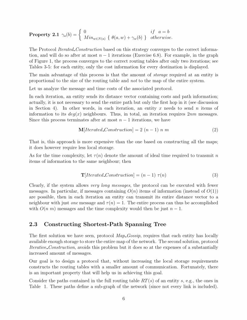
Property 2.1 γa(b) =

0 if a = bMinw∈N(a) θ(a, w) + γw(b) otherwise.

The Protocol Iterated Construction based on this strategy converges to the correct informa-tion, and will do so after at most n− 1 iterations (Exercise 6.8). For example, in the graphof Figure 1, the process converges to the correct routing tables after only two iterations; seeTables 3-5: for each entity, only the cost information for every destination is displayed.

The main advantage of this process is that the amount of storage required at an entity isproportional to the size of the routing table and not to the map of the entire system.

Let us analyze the message and time costs of the associated protocol.

In each iteration, an entity sends its distance vector containing costs and path information;actually, it is not necessary to send the entire path but only the first hop in it (see discussionin Section 4). In other words, in each iteration, an entity x needs to send n items ofinformation to its deg(x) neighbours. Thus, in total, an iteration requires 2nm messages.Since this process terminates after at most n− 1 iterations, we have

M[Iterated Construction] = 2 (n− 1) n m (2)

That is, this approach is more expensive than the one based on constructing all the maps;it does however require less local storage.

As for the time complexity, let τ(n) denote the amount of ideal time required to transmit nitems of information to the same neighbour; then

T[Iterated Construction] = (n− 1) τ(n) (3)

Clearly, if the system allows very long messages, the protocol can be executed with fewermessages. In particular, if messages containing O(n) items of information (instead of O(1))are possible, then in each iteration an entity can transmit its entire distance vector to aneighbour with just one message and τ(n) = 1. The entire process can thus be accomplishedwith O(n m) messages and the time complexity would then be just n− 1.

2.3 Constructing Shortest-Path Spanning Tree

The first solution we have seen, protocol Map Gossip, requires that each entity has locallyavailable enough storage to store the entire map of the network. The second solution, protocolIterative Construction, avoids this problem but it does so at the expenses of a substantiallyincreased amount of messages.

Our goal is to design a protocol that, without increasing the local storage requirementsconstructs the routing tables with a smaller amount of communication. Fortunately, thereis an important property that will help us in achieving this goal.

Consider the paths contained in the full routing table RT (s) of an entity s, e.g., the ones inTable 1. These paths define a sub-graph of the network (since not every link is included).

6

This sub-graph is special: it is connected, contains all the nodes, and does not have cycles(see Figure 1 where the subgraph links are in bold); in other words,

it is a spanning tree !

It is called the shortest-path spanning-tree rooted in s (PT (s)), sometimes known also as thesink tree of s.

This fact is important because it tell us that, to construct the routing table RT (s) of s, wejust need to construct the shortest-path spanning-tree PT (s).

2.3.1 Protocol Design

To construct the shortest-path spanning-tree PT (s), we can adapt a classical serial strategyfor constructing PT (s) starting from the source s:

Serial Strategy

• We are given a connected fragment T of PT (s), containing s (initially, T will becomposed of just s).

• Consider now all the links going outside of T (i.e., to nodes not yet in T ). To eachsuch link (x, y) associate the value v(x, y) = γs(x) + θ(x, y); i.e., v(x, y) is the cost ofreaching y from the source s by first going to x (through a shortest path) and thenusing the link (x, y) to reach y.

• Add to T the link (a, b) for which v(a, b) is minimum; in case of a tie, choose the oneleading to the node with the lexicographically smallest name.

The reason this strategy works is because of the following property:

Property 2.2 Let T and (a, b) be as defined in the Serial Strategy. Then T ∪ (a, b) is aconnected fragment T of PT (s).

That is, the new tree, obtained by adding the chosen (a, b) to T , is also a connected fragmentof PT (s), containing s; and it is clearly larger than T . In other words, using this strategy,the shortest-path spanning-tree PT (s) will be constructed, starting from s, by adding theappropriate links, one at the time.

The algorithm based on this strategy will be a sequence of iterations started from the root.In each iteration, the outgoing link (a, b) with minimum cost v(a, b) is chosen; the link (a, b)and the node b are added to the fragment, and a new iteration is started. The processterminates when the fragment includes all the nodes.

Our goal is now to implement this algorithm efficiently in a distributed way.

7

First of all, let us consider what a node y in the fragment T knows. Definitely y knows whichof its links are part of the current fragment; it also knows the length γs(y) of the shortestpath from the source s to it.

IMPORTANT. Let us assume for the moment that y also knows which of its links areoutgoing (i.e., lead to nodes outside of the current fragment), and which are internal.

In this case, to find the outgoing link (a, b) with minimum cost v(a, b) is rather simple, andthe entire iteration is composed of four easy steps:

Iteration

1. The root s broadcasts in T the start of the new iteration.

2. Upon receiving the start, each entity x in the current fragment T computes locallyv(x, y) = γs(x) + θ(x, y) for each of its outgoing incident links (x, y); it then selectsamong them the link e = (x, y′) for which v(x, y′) is minimized.

3. The overall minimum v(a, b) among all the locally selected v(e)’s is computed at s,using a minimum-finding for (rooted) trees (e.g., see Sect. ??), and the correspondinglink (a, b) is chosen as the one to be added to the fragment.

4. The root s notifies b of the selection; the link (a, b) is added to the spanning-tree; bcomputes γs(b), and s is notified of the end of the iteration.

Each iteration can be performed efficiently, in O(n) messages, since each operation (broad-cast, min-finding, notifications) are performed on a tree of at most n nodes.

There are a couple of problems that need to be addressed. A small problem is how can bcompute γs(b). This value is actually determined at s by the algorithm in this iteration;hence, s can communicate it to b when notifying it of its selection.

A more difficult problem regards the knowledge of which links are outgoing (i.e., they leadto nodes outside of the current fragment); we have assumed that an entity in T has such aknowledge about its links. But how can such a knowledge be ensured ?

As described, during an iteration, messages are sent only on the links of T and on the linkselected in that iteration. This means that the outgoing links are all unexplored (i.e., nomessage has been sent or received on them). Since we do not know which are outgoing,an entity could perform the computation of Step 2 for each of its unexplored incident linksand select the minimum among those. Consider for example the graph of Figure 2(a) andassume that we have already constructed the fragment shown in Figure 2(b). There are fourunexplored links incident to the fragment (shown as leading to square boxes), each with itsvalue (shown in the corresponding square box); the link (s, e) among them has minimumvalue and is chosen; it is outgoing and it is added to the segment. The new segment is shownin Figure 2(c) together with the unexplored links incident on it.

However, not all unexplored links are outgoing: an unexplored link might be internal (i.e.,leading to a node already in the fragment), and selecting such a link would be an error. For

8

5

5

33

10

1

3

2

8

5

3

10

1

33

53

3

8

5

10

1

3

5

10

1

3

5

8

5

3

(a) (b)

(c) (d)

s

h k

c d

f

e

7

9

10

10

es

h k

7

8

8

13

9

10

e

13

8

9

s

h k

5

s

h k

Figure 2: Determining the next link to be added to the fragment.

example, in Figure 2(c), the unexplored link (e, k) has value v(e, k) = 7 which is minimumamong the unexplored edges incident on the fragment, and hence would be chosen; however,node e is already in the fragment.

We could allow for errors: we choose among the unexplored links and, if the link (in ourexample: (e, k)) selected by the root s in step 3 turns out to be internal (k would find outin step 4 when the notification arrives), we eliminate that link from consideration and selectanother one. The drawback of this approach is its overall cost. In fact, since initially alllinks are unexplored, we might have to perform the entire selection process for every link.This means that the cost will be O(nm), which in the worst case is O(n3): a high price toconstruct a single routing table.

A more efficient approach is to add a mechanism so no error will occur. Fortunately, thiscan be achieved simply and efficiently as follows.

When a node b becomes part of the tree, it sends a message to all its neighbours notifyingthem that it is now part of the tree. Upon receiving such a message, a neighbour c knowsthat this link must no longer be used when performing shortest path calculations for thetree. As a side effect, in our example, when the link (s, e) is chosen in Figure 2(b), node eknows already that the link (e, k) leads to a node already in the fragment; thus such a linkis thus not considered, as shown in Figure 2(d).

RECALL. We have used a similar strategy with the protocol for Depth First Traversal, todecrease its time complexity.

IMPORTANT. It is necessary for b to ensure that all its neighbours have received itsmessage before a new iteration is started. Otherwise, due to time delays, a neighbour c

9

might receive the request to compute the minimum for the next iteration before the messagefrom b has even arrived; thus, it is possible that c (not knowing yet that b is part of the tree)chooses its link to b as its minimum, and such a choice is selected as the overall minimumby the root s. In other words, it is still possible that an internal link is selected during aniteration.

Summarizing, to avoid mistakes, it is sufficient to modify rule 4 as follows:

• 4’. The root s sends an Expand message to b and the link (a, b) is added to thespanning-tree; b computes γs(b), sends a notification to its neighbours, waits for theiracknowledgment, and then notifies s of the end of the iteration.

This ensures that there will be only n−1 iterations, each adding a new node to the spanning-tree, with a total cost of O(n2) messages. Clearly we must also consider the cost of eachnode notifying its neighbours (and them sending acknowledgments), but this adds only O(m)messages in total.

The protocol, called PT Construction, is shown in Figures 3-6.

2.3.2 Analysis

Let us now analyze the cost of protocol PT Construction in details. There are two ba-sic activities being performed: the expansion of the current fragment of the tree, and theannouncement (with acknowledgments) of the addition of the new node to the fragment.

Let us consider the expansion first. It consists of a “start-up” (the root broadcasting theStart Iteration message), a “convergecast” (the minimum value is collected at the root usingthe MinValue messages), two “notifications” (the root notifies the new node using the Ex-pansion message, and the new node notifies the root using the Iteration Completed message).Each of these operations are performed on the current fragment which is a tree, rooted inthe source. In particular, the start-up and the convergecast operations each cost only onemessage on every link; in the notifications, messages are sent only on the links in path fromthe source to the new node, and there will be only one message in each direction. Thus, intotal, on each link of the tree constructed so far, there will be at most four messages due tothe expansion; two messages will also be sent on the new link added in this expansion. Thusin the expansion at iteration i, at most 4(ni − 1) + 2 messages will be sent, where ni is thesize of the current tree. Since the tree is expanded by one node at the time, ni = i: initiallythere is only the source; then the fragment is composed of the source and a neighbour, andso on. Thus, the total number of messages due to the expansion is

∑n−1i=1 (4(ni − 1) + 2) =

∑n−1i=1 (4i− 2) = 2n(n− 1)− 2(n− 1) = 2n2 − 4n + 2

The cost due to announcements and acknowledgments is simple to calculate: each node willsend a Notify message to all its neighbours when it becomes part of the tree, and receivesan Ack from each of them. Thus, the total number of messages due to the notifications is

2∑

x∈V |N(x)| = 2∑

x∈V deg(x) = 4m

10

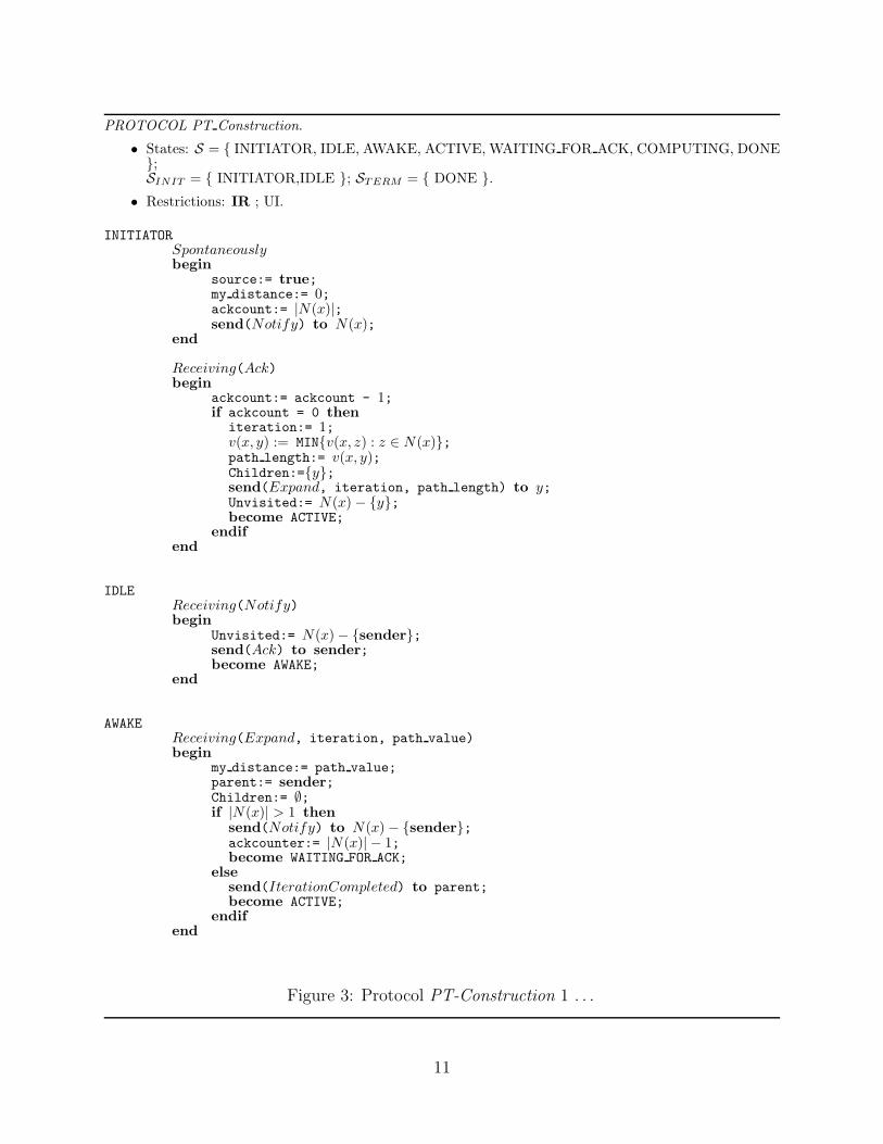
PROTOCOL PT Construction.

• States: S = INITIATOR, IDLE, AWAKE, ACTIVE, WAITING FOR ACK, COMPUTING, DONE;SINIT = INITIATOR,IDLE ; STERM = DONE .

• Restrictions: IR ; UI.

INITIATORSpontaneouslybegin

source:= true;my distance:= 0;ackcount:= |N(x)|;send(Notify) to N(x);

end

Receiving(Ack)begin

ackcount:= ackcount - 1;if ackcount = 0 then

iteration:= 1;v(x, y) := MINv(x, z) : z ∈ N(x);path length:= v(x, y);Children:=y;send(Expand, iteration, path length) to y;Unvisited:= N(x) − y;become ACTIVE;

endifend

IDLEReceiving(Notify)begin

Unvisited:= N(x)− sender;send(Ack) to sender;become AWAKE;

end

AWAKEReceiving(Expand, iteration, path value)begin

my distance:= path value;parent:= sender;Children:= ∅;if |N(x)| > 1 then

send(Notify) to N(x)− sender;ackcounter:= |N(x)| − 1;become WAITING FOR ACK;

elsesend(IterationCompleted) to parent;become ACTIVE;

endifend

Figure 3: Protocol PT-Construction 1 . . .

11

AWAKEReceiving(Notify)begin

Unvisited:= Unvisited−sender;send(Ack) to sender;

end

WAITING FOR ACKReceiving(Ack)begin

ackcount:= ackcount - 1;if ackcount = 0 then

send(IterationCompleted) to parent;become ACTIVE;

endifend

ACTIVEReceiving(Iteration Completed)begin

if not(source) thensend(Iteration Completed) to parent;

elseiteration:= iteration + 1;send(Start Iteration, iteration) to children;Compute Local Minimum;childcount:= 0;become COMPUTING;

endifend

Receiving(Start Iteration, counter)begin

iteration:= counter;Compute Local Minimum;if children = ∅ then

send(MinV alue, minpath) to parent;else

send(Start Iteration, iteration) to children;childcount:=0;become COMPUTING;

endifend

Figure 4: Protocol PT-Construction 2. . .

12

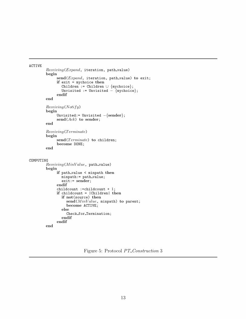
ACTIVEReceiving(Expand, iteration, path value)begin

send(Expand, iteration, path value) to exit;if exit = mychoice then

Children := Children ∪ mychoice;Unvisited := Unvisited − mychoice;

endifend

Receiving(Notify)begin

Unvisited:= Unvisited −sender;send(Ack) to sender;

end

Receiving(Terminate)begin

send(Terminate) to children;become DONE;

end

COMPUTINGReceiving(MinV alue, path value)begin

if path value < minpath thenminpath:= path value;exit:= sender;

endifchildcount :=childcount + 1;if childcount = |Children| then

if not(source) thensend(MinV alue, minpath) to parent;become ACTIVE;

elseCheck for Termination;

endifendif

end

Figure 5: Protocol PT Construction 3

13

Procedure Check for Terminationbegin

if minpath= inf thensend(Terminate) to Children;become DONE;

elsesend(Expand, iteration, minpath) to exit;become ACTIVE;

endifend

Procedure Compute Local Minimumbegin

if Unvisited = ∅ thenminpath:= inf;

elselink length:= v(x, y) = MINv(x, z) : z ∈ Unvisited;minpath:= my distance + link length;mychoice:= exit:= y;

endifend

Figure 6: Procedures used by protocol PT Construction

To complete the analysis, we need to consider the final broadcast of the Termination messagewhich is performed on the constructed tree; this will add n−1 messages to the total, yieldingthe following:

M[PT Construction] ≤ 2n2 − 4n + 2 + 4m + n− 1 = 2n2 + 4m− 3n + 1 (4)

By adding a little bookkeeping, the protocol can be used to construct the routing tableRT (s) of the source (Exercise 6.13). Hence, we have a protocol which constructs the routingtable of a node using O(n2) messages.

We will see later how more efficient solutions can be derived for the special case when allthe links have the same cost (or, alternatively, there is no cost on the links).

Note that we have made no assumptions other that the costs are not-negative; in particular,we did not assume FIFO channels (i.e., message ordering).

2.3.3 Constructing All Routing Tables

Protocol PT Construction allows us to construct the shortest-path tree of a node, and thusto construct the routing table of that entity. To solve the original problem of constructingall the routing table, also known as all-pairs shortest-paths construction, this process mustbe repeated for all nodes. The complexity of resulting protocol PT All follows immediatelyfrom equation 4:

14

Algorithm Cost restrictions

Map Gossip O(n m) Ω(m) local storageIterative Construction O(n2 m)

PT O(n3)

Table 6: Summary: Costs of constructing all shortest-path routing tables.

M[PT All] ≤ 2n3 − 3n2 + 4(m− 1)n (5)

It is clear that some information computed when constructing PT (x) can be re-used in theconstruction of PT (y). For example, the shortest path from x to y is just the reverse of theone from y to x (under the bidirectional links assumption we are using); hence we just needto determine one of them. Even stronger is the so-called optimality principle:

Property 2.3 If a node x is in the shortest path π from a to b, then π is also a fragmentof PT (x)

Hence, once a shortest path π has been computed for the shortest path tree of an entity,this path can be added to the shortest path tree of all the entities in the path. So, in theexample of Figure 1, the path (s, e)(e, f) in PT (s) will also be part of PT (e) and PT (f).However, to date, it is not clear how this fact can be used to derive a more efficient protocolfor constructing all the routing tables.

A summary of the results we have discussed is shown in Table 6

In systems that allow very long messages, not-surprisingly the problem can be solved withfewer messages. For example, if messages can contain O(n) items of information (insteadof O(1)), all the shortest-path trees can be constructed with just O(n2) messages (Exercise6.15). If messages can contain O(n2) items then, as discussed in Section ??, any graph prob-lem including the construction of all shortest-path trees can be solved using O(n) messagesonce a leader has been elected (requiring at least O(m + mlogn) normal messages).

2.4 Min-Hop Routing

Consider the case when all links have the same cost (or alternatively, there are no costsassociated to the links); that is, θ(a, b) = θ for all (a, b) ∈ E.

This case is special in several respects. In particular, observe that the shortest path from ato b will have cost γa(b) = θ dG(a, b), where dG(a, b) is the distance (in number of hops) of afrom b in G; in other words, the cost of a path will depend solely on the number of hops (i.e.,the number of links) in that path. Hence, the shortest-path between two nodes will be theone of minimum hops. For these reasons, routing in this situation is called min-hop routing.

An interesting consequence is that the shortest-path spanning-tree of a node coincides withits breadth-first spanning-tree ! In other words, a breadth-first spanning-tree rooted in a nodeis the shortest-path spanning-tree of that node when all links have the same cost.

15

Protocol PT Construction works for any choice of the costs, provided they are non-negative,so it constructs a breadth-first spanning-tree if all the costs are the same. However, wecan take advantage of the fact that all links have the same costs to obtain a more efficientprotocol. Let us see how.

2.4.1 Breadth-First Spanning Tree Construction

Without any loss of generality, let us assume that θ = 1; thus, γs(a) = dG(s, a).

We can use the same strategy of protocol PT Construction of starting from s and successivelyexpanding the fragment; only, instead of choosing one link (and thus one node) at the time,we can choose several simultaneously: in the first step, s chooses all the nodes at distance1 (its neighbours); in the second step, s chooses simultaneously all the nodes at distance 2;in general, in step i, s chooses simultaneously all the nodes at distance i; notice that, beforestep i, none of the nodes at distance i were part of the fragment. Clearly, the problem is todetermine, in step i, which nodes are at distance i from s.

Observe this very interesting property: all the neighbours of s are at distance 1 from s; alltheir neighbours (not at distance 1 from s) are at distance 2 from s; in general

Property 2.4 If a node is at distance i from s, then its neighbours are at distance eitheri− 1 or i or i + 1 from s.

This means that, once the nodes at distance i from s have been chosen (and become part ofthe fragment), we need to consider only their neighbours to determine which nodes are atdistance i + 1.

So the protocol, which we shall call BF, is rather simple. Initially, the root s sends a “Startiteration 1”message to each neighbor indicating the first iteration of the algorithm, andconsiders them its children. Each recipient marks its distance as 1, marks the sender as itsparent, and sends an acknowledgment back to the parent. The tree is now composed of theroot s and its neighbours, which are all at distance 1 from s.

In general, after iteration i all the nodes at distance up to i are part of the tree. Furthermore,each node at distance i knows which of its neighbours are at distance i− 1 (Exercise 6.16).

In iteration i + 1, the root broadcasts on the current tree a “Start iteration i + 1” message.Once this message reaches a node x at distance i, it will send a ”Explore i + 1” message toits neighbours that are not at distance i− 1 (recall, x knows which they are), and waits fora reply from each of them. These neighbours are either at distance i like x itself, or i + 1;those at distance i are already in the tree so do not need to be included. Those at distancei + 1 must be attached to the tree; however, each must be attached only once (otherwise wecreate a cycle and do not form a tree). See Figure 7.When a neighbour y receives the ”Explore” message, the content of its reply will dependon whether or not y is already part of the tree. If y is not part of the tree, it now knowsthat it is at distance i + 1 from s; it then marks the sender as its parent, sends a positiveacknowledgment to it, and becomes part of the tree. If y is part of the tree (even if it just

16

happened in this iteration), it will reply with a negative acknowledgment.When x receives the reply from y: if the reply is positive, it will mark y as a child; otherwise,it will mark y as already in the tree. Once all the replies have been received, it participatesin a convergecast notifying the root that the iteration has been completed.

t + 1

t

s

Figure 7: Protocol BH expands an entire level in each iteration.

CostLet us now examine the cost of protocol BF. Denote by ni the number of nodes at distanceat most i from s. In each iteration, there are three operations involving communication: (1)the broadcast of “Start”on the tree constructed so far; (2) the sending of ”Explore” messagessent by the nodes at distance i, and the corresponding replies; and (3) the convergecast tonotify the root of the termination of the iteration.

Consider first the cost of operation (2), that is the cost of the ”Explore” messages and thecorresponding replies. Consider a node x at distance i. As already mentioned, its neighboursare at distance either i− 1 or i or i + 1. The neighbours at distance i− 1 sent an ”Explore”message to x in stage i− 1, so x sent a reply to each of them. In stage i x sent an ”Explore”message to all its other neighbours. Hence, in total, x sent just one message (either ”Explore”or reply) to each of its neighbours. This means that, in total, the number of ”Explore” and“Reply” messages is

∑

x∈V | N(x)‖ = 2m

We will consider now the overall cost of operations (1) and (3). In iteration i + 1, both thebroadcast and convergecast are performed on the tree constructed in iteration i, thus costingni − 1 messages each, for a total of 2ni − 2 messages. Therefore, the total cost will be

∑

1≤i<r(s) 2(ni − 1)

where r(s) denotes the eccentricity of s (i.e., the hight of the breadth-first spanning tree ofs).

17

Summarizing

M[BF ] ≤ 2m +∑

1≤i<r(s)

2(ni − 1) ≤ 2m + 2(n− 1) d(G) (6)

where d(G) is the diameter of the graph. We know that ni < ni+1 and that nr(s) = n inany network G and for any root s, but the actual values depend on the nature of G andon the position of s. For example, in the complete graph, r(s) = 1 for any s, so the entireconstruction is completed in the first iteration; however, m = n(n−1)/2; hence the cost willbe

n(n− 1) + 2(n− 1) = n2 + n− 2

On the other hand, if G is a line and s is an endpoint of the line, r(s) = n− 1 and in eachiteration we only add one node (i.e., ni = i); thus

∑

1≤i<r(s) 2(ni− 1) = n2− 4n+3; howeverm = n− 1 hence the cost will be

2(n− 1) + n2 − 4n + 3 = n2 − 2n + 1

As for the time complexity, in iteration i, the “Start” messages travel from the root s to thenodes at distance i − 1, hence arriving there after i − 1 time units; therefore, the nodes atdistance i will receive the ”Explore i” message after i time units. At that time, they will startthe convergecast to notify the root of the termination of the iteration; this process requiresexactly i time units. In other words, iteration i will cost exactly 2i time units. Summarizing

T[BF ] = 2∑

1≤i≤r(s)

i = r(s)(r(s) + 1) ≤ d(G)2 + d(G) (7)

2.4.2 Multiple Layers: An Improved Protocol

To improve the costs, we must understand the structure of protocol BF. We know that itsexecution of protocol BF is a sequence of iterations, started by the root.

Each iteration i + 1 of protocol BF can be thought of as composed of three different phases:

1. Initialization: the root node broadcasts the “Start iteration i + 1” along the alreadyconstructed tree, which will reach the leaves (i.e., the nodes at distance i from theroot).

2. Expansion: in this phase, which is started by the leaves, new nodes (i.e., all those oflevel i + 1) are added to the tree forming a larger fragment.

3. Termination: the root is notified of the end of this iteration using a convergecast onthe new tree.

18

Initialization and termination are bookkeeping operations that allow the root to somehowsynchronize the execution of the algorithm, iteration by iteration. For this reason, the two ofthem, together, are also called synchronization. Each synchronization costs O(n) messages(since it is done on a tree). Hence, this activity alone costs

O(nL)

messages where L is the number of iterations.

In the original protocol BF, we expand the tree one level at the time; hence L = deg(G)and the total cost for synchronization alone is O(n deg(G)) messages (see expression 6).This means that, to reduce the cost of synchronization, we need to decrease the number ofiterations. To do so, we need each iteration to grow the current tree by more than a singlelevel; that is, we need each expansion phase to add several levels to the current fragment.

Let us see how to expand the current tree by l ≥ 1 levels, in a single iteration, efficiently(see Figure 8). Assume that initially each node x 6= r has a variable levelx = ∞, whilelevelr = 0.

t + l

t + 2

t + 1

t

s

l

Figure 8: Protocol BF Levels expands l levels in each iteration.

Let t be the current level of the leaves; each leaf will start the exploration by sendingExplore(t + 1, l) to its still unexplored neighbours. In general, the expansion messages willbe of the form Explore(level, counter), where level is the next level to be assigned and counterdenotes how many more levels should be expanded by the node receiving the message.

When a node x not yet in the tree receives its first expansion message, say Explore(j, k) fromneighbour y, it will accept the message, consider the sender y as its parent in the tree, andset its own level to be j. It then considers the number k of levels still to be expanded. Ifk = 0, x sends immediately a Positive(j) reply to its parent y. Instead, if k > 0, x will sendExplore(j + 1, k − 1) to all its other neighbours, and wait for their reply: those that reply

19

Positive(j + 1) are considered its children, those that reply Negative(j + 1) are considerednot-children; if/when all have sent a reply with level j + 1, x sends a Positive(j) reply to itsparent y.

Note that this first “Explore” message will not necessarily determine x’s parent or level inthe final tree; in fact, it is possible that x will receive later an Explore(j′, k′) message witha smaller level j′ < j from a neighbour z. (Note: it might even be possible that y = z).What we will do in this case is to have x “trow away” the work already done and “start fromscratch” with the new information: x will accept the message, consider z its parent, set itslevel to j′, send Explore(j′ +1, k′−1) to all its other neighbours (assuming k′ > 0), and waitfor their reply. Note that x might have to “trow away” work already done more than onceduring an iteration. How many times ? It is not difficult to figure out that it can happen atmost t− j + 1 times, where j is the first level it receives in this iteration (Exercise 6.19).

We still have to specify under what conditions will a node x send a negative reply to areceived message Explore(j, k); the rule is simple: x will reply Negative(j) if no shorter pathis found from the root s to x, i.e. if j ≥ levelx.

A more detailed description of the expansion phase of the protocol, which we will callBF Levels, is shown in Figure 9, describing the behaviour of a node x not part of thecurrent fragment. As mentioned, the expansion phase is started by the leaves of the currentfragment, which we will call sources of this phase, upon receiving the Start Iteration messagefrom the root. Each source will then send Explore(t + 1, l) to their unexplored neighbours,where t is the level of the leaves and l (a design parameter) is the number of levels that willbe added to the current fragment in this iteration. The terminating phase also is started bythe sources (i.e., the leaves of the already existing fragment), upon receiving a reply to alltheir expansion messages.

CorrectnessDuring the extension phase all the nodes at distance at most t + l from the root are indeedreached, as can be easily verified (Exercise 6.20). Thus, to prove the correctness of theprotocol we need just to prove that those nodes will be attached to the existing fragment atthe proper level.

We will prove this by induction on the levels. First of all, all the nodes at level t + 1 areneighbours of the sources and thus each will receive at least one Explore(t + 1, l) message;when this happens, regardless of whatever has happened before, each will set its level tot + 1; since this is the smallest level that they can ever receive, their level will not changeduring the rest of the iteration.

Let it be true for the nodes up to level t + k, 1 ≤ k ≤ l − 1; we will show that it holdsalso for the nodes in level t + k + 1. Let π be the path of length t + k + 1 from s to x andlet u be the neighbour of x in this path; by definition, u is at level t + k and, by inductivehypothesis, it has correctly set (levelu) = t + k. When this happened, u sent a messageExplore(t + k + 1, l − k − 1) to all its neighbours, except its parent. Since x is clearly notu’s parent, it will eventually receive this message; when this happens, x will correctly set(levelx) = t + k + 1. So we must show that the expansion phase will not terminate before x

20

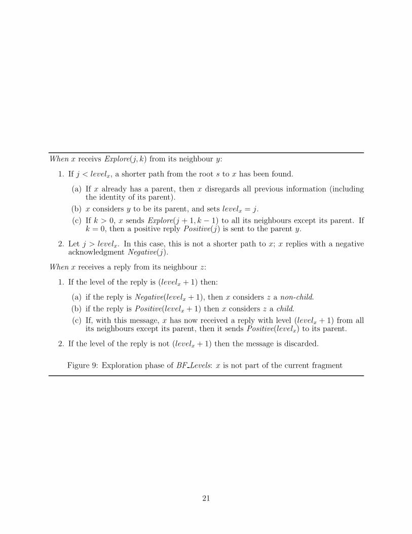
When x receivs Explore(j, k) from its neighbour y:

1. If j < levelx, a shorter path from the root s to x has been found.

(a) If x already has a parent, then x disregards all previous information (includingthe identity of its parent).

(b) x considers y to be its parent, and sets levelx = j.

(c) If k > 0, x sends Explore(j + 1, k − 1) to all its neighbours except its parent. Ifk = 0, then a positive reply Positive(j) is sent to the parent y.

2. Let j > levelx. In this case, this is not a shorter path to x; x replies with a negativeacknowledgment Negative(j).

When x receives a reply from its neighbour z:

1. If the level of the reply is (levelx + 1) then:

(a) if the reply is Negative(levelx + 1), then x considers z a non-child.

(b) if the reply is Positive(levelx + 1) then x considers z a child.

(c) If, with this message, x has now received a reply with level (levelx + 1) from allits neighbours except its parent, then it sends Positive(levelx) to its parent.

2. If the level of the reply is not (levelx + 1) then the message is discarded.

Figure 9: Exploration phase of BF Levels: x is not part of the current fragment

21

receives this message. Focus again on node u; it will not send a positive acknowledgment toits parent (and thus the phase can not terminate) until it receives a reply from all its otherneighbours, including x. Since, to reply, x must first receive the message, x will correctly setits level during the phase.

Cost

To determine the cost of protocol BF Levels, we need to analyze the cost of the synchroniza-tion and of the expansion phases.

The cost of a synchronization, as we discussed earlier, is at most 2(n−1) messages, since boththe initialization broadcast and the termination convergecast are performed on the currentlyavailable tree. Hence, the total cost of all synchronizations activities depends on the numberof iterations. this quantity is easily determined. Since there are radius(r) < d(G) levels,and we add l levels in every iterations, except in the last where we add the rest, the numberof iterations is at most ⌈d(G)/l⌉. This means that the total amount of messages due tosynchronization is at most

2(n− 1) ⌈ d(G)

l⌉ ≤ 2

(n− 1)2

l(8)

Let us now analyze the cost of the expansion phase in iteration i, 1 ≤ i ≤ ⌈d(G)/l⌉. Observethat, in this phase, only the nodes in the levels L(i) = (i−1)l+1, (i−1)l+2, . . . , il−1, ilas well as the sources (i.e., the nodes at level (i − 1)l) will be involved, and messages willonly be sent on the mi links between them. The messages sent during this phase will bejust Explore(t + 1, l), Explore(t + 2, l− 1), Explore(t + 3, l− 2),. . . ,Explore(t + l, 0), and thecorresponding replies, Positive(j) or Negative(j), t + 1 ≤ j ≤ t + l.

A node in one of the levels in L(i) sends to its neighbours at most one of each of thoseExplore messages; hence there will be on each of edge at most 2l Explore messages (l in eachdirection), for a total of 2lmi. Since for each Explore there is at most one reply, the totalnumber of messages sent in this phase will be no more than 4lmi This fact, observing thatthe set of links involved in each iteration are disjoint, yields less than

⌈d(G)/l⌉∑

i=1

4 l mi = 4 l m (9)

messages for all the explorations of all iterations. Combining (8) and (9), we obtain

M[BF Levels] ≤ 2(n− 1)d(G)

l+ 4 l m (10)

If we choose l = O(n/√

m), expression (10) becomes

M[BF Levels] = O(n√

m)

22

Network Algorithm Messages Time

General BF O(m + nd) O(d2)General BF Levels O(n

√m) O(d2√m/n + d)

Planar BF Levels O(n1.5) O(d2/√

n + d)

Table 7: Summary: Costs of constructing a breadth-first tree.

This formula is quite interesting. In fact, it depends not only on n but also on the squareroot of the number m of links.

If the network is sparse (i.e., it has O(n) links), then the protocol uses only

O(n1.5)

messages; note that this occurs in any planar network.

The worst case will be with very dense networks (i.e., m = O(n2)). However in this case theprotocol will use at most

O(n2)

messages, which is no more than protocol BF .

In other words, protocol BF Levels will have the same cost as protocol BF only for very densenetworks, and will be much better in all other systems; in particular, whenever m = o(n2),it uses a subquadratic number of messages.

Let us consider now the ideal time costs of the protocol. Iteration i consists of reaching levelsL(i) and returning to the root; hence the ideal time will be exactly 2il if 1 ≤ i < ⌈d(G)/l⌉,and time 2d(G) in the last iteration. Thus, without considering the roundup, in total wehave

T[BF Levels] =

d(G)/l∑

i=1

2 l i =d(G)2

l+ d(G) (11)

The choice l = O(n/√

m) we considered when counting the messages will give

T[BF Levels] = O(d(G)2√

m/n)

which, again, is the same ideal time as protocol BF only for very dense networks, and lessin all other systems.

2.4.3 Reducing Time with More Messages

If time is of paramount importance, better results can be obtained at the cost of moremessages. For example, if in protocol BF Levels we were to choose l = d(G), we wouldobtain an optimal time costs.

23

T[BF Levels] = 2d(G)

IMPORTANT. We measure ideal time considering a synchronous execution where thecommunication delays are just one unit of time. In such an execution, when l = d(G), thenumber of messages will be exactly 2m + n − 1 (Exercise 6.22). In other words, in thissynchronous execution, the protocol has optimal message costs. However, this is not themessage complexity of the protocol, just the cost of that particular execution. To measurethe message complexity we must consider all possible executions. Remember: to measureideal time we consider only synchronous executions, while to measure message costs we mustlook at all possible executions, both synchronous and asynchronous (and choose the worstone).

The cost in messages choosing l = d(G) is given by expression (10) that becomes

O(m d(G))

This quantity is reasonable only for networks of small degree. By the way, a priori knowledgeof d(G) is not necessary to obtain these bounds (either time or messages): Exercise 6.21.

If we are willing to settle for a low but suboptimal time, it is possible to achieve it with abetter message complexity. Let us how.

In protocol BF Levels the network (and thus the tree) is viewed as divided into “strips”,each containing l levels of the tree. See Figure 10.

l

l

l

l

l

s

Figure 10: We need more efficient expansion of l levels in each iteration.

The way the protocol works right now, in the expansion phase, each source (i.e., each leaf ofthe existing tree) constructs its own bf-tree over the nodes in the next l levels. These bf-treeshave differential growth rates, some growing quickly, some slowly. Thus, it is possible for aquickly growing bf-tree to have processed many more levels than a slower bf-tree. Wheneverthere are conflicts due to transmission delays (e.g., the arrival of a message with a better

24

level) or to concurrency (e.g., the arrival of another message with the same level), theseconflicts are resolved, either by “trowing away” everything already done and joining the newtree, or sending a negative reply. It is the amount of work performed to take care of theseconflicts that drives the costs of the protocol up. For example, when a node joins a bf-treeand has a (new) parent, it must send out messages to all its other neighbours; thus, if anode has a high degree and frequently changes trees, these adjacent edge messages dominatethe communication complexity. Clearly the problem is how to perform these operationsefficiently.

Conflicts and overlap occurring during the constructions of those different bf-trees in the llevels can be reduced by organizing the sources into clusters and coordinating the actions ofthe sources that are in the same cluster, as well as coordinating the different clusters.

This in turn requires that the sources in the same cluster must be connected so to minimizethe communication costs among them. The connection through a tree is the obvious option,and is called a cover tree. To avoid conflicts, we want that for different clusters the corre-sponding cover trees have no edges in common. So we will have a forest of cover trees, whichwe will call the cover of all the sources. To coordinate the different clusters in the coverwe must be able to reach all sources; this however can already be done using the currentfragment (recall, the sources are the leaves of the fragment).

The message costs of the expansion phase will grow with the number of different clusterscompeting for the same node (the so-called load factor); on the other hand, the time costswill grow with the depth of the cover trees (the so-called depth factor). Notice that it ispossible to obtain tradeoffs between the load factor and the depth factor by varying the sizeof the cover (i.e., the number of trees in the forest); e.g., increasing the size of the forestreduces the depth factor while increasing the load factor.

We are thus faced with the problem of constructing clusters with small amount of competitionand shallow cover trees. Achieving this goal yields a time cost of O(d1+ǫ) and a message costof O(m1+ǫ) for any fixed ǫ > 0. See Exercise 6.23.

2.5 Suboptimal Solutions: Routing Trees

Up to now, we have considered only shortest-path routing; that is, we have been lookingat systems that always route a message to its destination through the shortest-path. Wewill call such mechanisms optimal. To construct optimal routing mechanisms, we had toconstruct n shortest-path trees, one for each node in the network, a task that we have seenis quite communication expensive.

In some cases, the shortest path requirement is important but not crucial; actually, in manysystems, guarantee of delivery with few communication activities is the only requirement.

If the shortest-path requirement is relaxed or even dropped, the problem of constructinga routing mechanism (tables and forwarding scheme) becomes simpler and can be achievedquite efficiently. Because they do not guarantee shortest-paths, such solutions are called sub-optimal. Clearly there are many possibilities depending on what (sub optimal) requirementsthe routing mechanism must satisfy.

25

A particular class of solutions is the one using a single spanning-tree of the network for all therouting, which we shall call routing tree. The advantages of such an approach is obvious: weneed to construct just one tree. Delivery is guaranteed and no more that diam(T ) messageswill be used on the tree T . Depending on which tree is used, we have different solutions. Letus examine a few.

• Center-Based Routing. Since the maximum number of messages used to deliver amessage is at most diam(T ), a natural choice for a routing tree is the spanning tree withthe smallest diameter. Clearly, for any spanning tree T we have diam(T ) ≥ diam(G),so the best we can hope for is to select a tree that has the same diameter as thenetwork. One such a tree is shortest-path tree rooted in a center of the network. Infact, let c a center of G (i.e., a node where the maximum distance is minimized) andlet PT (c) be the shortest-path tree of c. Then (Exercise 6.24):

diam(G) = diam(PT (c))

To construct such a tree, we need first of all to determine a center c and then constructPT (c), e.g., using protocol PT Construction.

x y

T[x−y] T[y−x]

Figure 11: The message traffic between the two subtrees passes through edge e = (x, y).

• Median-Based Routing. Once we choose a tree T , an edge e = (x, y) of T linking thesubtree T [x−y] to the subtree T [y−x] will be used every time a node in T [x−y] wantsto send a message to a node in T [y − x], and viceversa (see Figure 11), where eachuse costs θ(e). Thus, assuming that overall every node generates the same amountof messages for every other node and all nodes overall generate the same amount ofmessages, the cost of using T for routing all this traffic is

Traffic(T ) =∑

(x,y)∈T |T [x− y]| |T [y − x]| θ(x, y)

It is not difficult to see that such a measure is exactly the sum of all distances betweennodes (Exercise 6.25). Hence, the best tree T to use is one that minimizes the sum ofall distances between nodes. Unfortunately, to construct the minimum-sum-distancespanning-tree of a network is not simple. In fact, the problem is NP-hard. Fortunately,it is not difficult to construct a near-optimal solution. In fact, let z be a median of thenetwork (i.e., a node for which the sum of distances SumDist(z) =

∑

v∈V dG(x, z) toall other nodes is minimized) and let PT (z) be the shortest-path tree of z. If T⋆ is thespanning tree that minimizes traffic, then traffic (Exercise 6.26):

26

Traffic(PT (z)) ≤ 2 Traffic(T⋆)

Thus, to construct such a tree, we need first of all to determine a median z and thenconstruct PT (z), e.g., using protocol PT Construction.

• Minimum-Cost Spanning-Tree Routing. A natural choice for routing tree is a minimum-cost spanning-tree (MST) of the network. The construction of such a tree can be donee.g., using protocol MegaMerger discussed in Chapter ??.

All the solutions above have different advantages; for example, the center-based one offersthe best worst-case cost, while the median-based one has the best average cost. Dependingon the nature of the systems and of the applications, each might be preferable to the others.

There are also other measures that can be used to evaluate a routing tree. For example, acommon measure is the so called stretch factor σG(T ) of a spanning-tree T of G defined as

σG(T ) = Maxx,y∈VdT (x, y)

dG(x, y)(12)

In other words, if a spanning-tree T has a stretch factor α, then for each pair of nodes xand y the cost of the path from x to y in T is at most α times the cost of the shortestpath between x and y in G. A design goal could thus be to determine spanning trees withsmall stretch factors (see Exercises 6.27 and 6.28). These ratio are sometimes be difficult tocalculate.

Alternate, easier to compute, measures are obtained by taking into account only pairs ofneighbours (instead of pairs of arbitrary nodes). One such measure is the so called dilation,that is the lenght of the longest path in the spanning-tree T corresponding to an edge of G,defined as

dilationG(T ) = Max(x,y)∈E dT (x, y) (13)

We also can define the edge-stretch factor ǫG(T ) (or dilation factor) of a spanning-tree T ofG as

ǫG(T ) = Max(x,y)∈EdT (x, y)

θ(x, y)(14)

As an example, consider the spanning-tree PT (c) used in the center-based solution; if all thelink costs are the same, we have that for every two nodes x and y

1 ≤ dG(x, y) ≤ dPT (c)(x, y) ≤ dPT (c) = dG

This means that in PT (c) (unweighted) stretch factor σG(T ), dilation dilationG(T ), andedge -stretch factor ǫG(T ) are all bounded by the same quantity, the diameter dG of G.

For a given spanning tree T , the stretch factor and the dilation factor measure the worstratio between the distance in T and in G for the same pair of nodes and the same edge,

27

respectively. Another important cost measures are the average stretch factor describing theaverage ratio:

σG(T ) = Averagex,y∈VdT (x, y)

dG(x, y)(15)

and the average edge-stretch factor (or average dilation factor) ǫG(T ) of a spanning-tree Tof G as

ǫG(T ) = Average(x,y)∈EdT (x, y)

θ(x, y)(16)

Construction of spanning trees with low average edge-stretch can be done effectively (Exer-cises 6.32 and 6.33).

Summarizing, the main disadvantage of using a routing tree for all routing tasks is the factthat the routing path offered by such mechanisms is not optimal. If this is not a problem,these solutions are clearly a useful and viable alternative to shortest-path routing.

The choice of which spanning tree, among the many, should be used depends on the natureof the system and of the application. Natural choices include the ones described above, aswell as those minimizing some of the cost measures we have introduced (see Exercises 6.28,6.29, 6.30).

3 Coping with Changes

In some systems, it might be possible that the cost associated to the links change over time;think for example of having a tariff (i.e., cost) for using a link during weekdays differentfrom the one charged in the weekend. If such a change occurs, the shortest path betweenseveral pairs of node might change, rendering the information stored in the tables obsoleteand possibly incorrect. Thus, the routing tables need to be adjusted.

In this section we will consider the problem of dealing with such events. We will assumethat, when the cost of a link (x, y) changes, both x and y are aware of the change and ofthe new cost of the link. In other words, we will replace the Total Reliability restriction withTotal Component Reliability (thus, the only changes are in the costs) in addition to the CostChange Detection restriction.

Note that costs that change in time can also describe the occurrence of some link failuresin the system: the crash failure of an edge can be described by having its cost becomingexceedingly large. Hence, in the following, we will talk of link crash failures and of costchanges as the same types of events,

3.1 Adaptive Routing

In these dynamical networks where cost changes in time, the construction of the routingtables is only the first step for ensuring (shortest-path) routing: there must be a mechanismto deal with the changes in the network status, adjusting the routing tables accordingly.

28

3.1.1 Map Update

A simple, albeit expensive solution is the Map Update protocol.

It requires first of all that each table contains the complete map of the entire network; thenext “hop” for a message to reach its destination is computed based on this map. Theconstruction of the maps can be done e.g. using protocol Map Gossip discussed in Section2.1. Clearly, any change will render the map inaccurate. Thus, integral part of this protocolis the update mechanism:

Maintenance

• as soon as an entity x detects a local change (either in the cost or in the status of anincident link), x will update its map accordingly and inform all its neighbours of thechange through an “update” message;

• as soon as an entity y receives an “update” from a neighbour, it will will update its mapaccordingly and inform all its neighbours of the change through an “update” message.

NOTE. In several existing systems, an even more expensive periodic maintenance mech-anism is used: Step 1 of the Maintenance Mechanism is replaced by having each node,periodically and even if there are no detected changes, send its entire map to all its neigh-bours. This is for example the case with the second Internet routing protocol: the completemap is being sent to all neighbours every 10 to 60 seconds (10 seconds if there is a costchange; 60 seconds otherwise).

The great advantage of this approach is that it is fully adaptive and can cope with anyamount and type of changes. The clear disadvantage is the amount of information requiredlocally and the volume of transmitted information.

3.1.2 Vector Update

To alleviate some of the disadvantages of the Map Update protocol, an alternative solutionconsists in using protocol Iterative Construction, that we designed to construct the routingtables, to keep them up-to-date should faults or changes occur. Every entity will just keepits routing table.

Note that a single change might make all the routing tables incorrect. To complicate things,changes are detected only locally, where they occur, and without a full map it might beimpossible to detect if it has any impact on a remote site; furthermore, if more severalchanges occur concurrently, their cumulative effect is unpredictable: a change might “undo”the damage inflicted to the routing tables by another change.

Whenever an entity x detects a local change (either in the cost or in the status of an incidentlink), the update mechanism is invoked which will trigger an execution of possibly severaliterations of protocol Iterative Construction.

In regards to the update mechanism, we have two possible choices:

29

• Recompute the routing tables: everybody starts a new execution of the algorithm,trowing away the current tables, or

• Update current information: everybody start a new iteration of the algorithm with xusing the new data, and continuing until the tables converge.

The first choice is very costly since, as we know, the construction of the routing tables is anexpensive process. For these reasons, one might want to recompute only what and when isnecessary; hence the second choice.

The second choice was used as the original Internet routing protocol; unfortunately, it hassome problems.

A well known problem is the so called count-to-infinity problem. Consider the simple networkshown in Figure 12. Initially all links have cost 1. Then the cost of link (z, w) becomes alarge integer K >> 1. Both nodes z and w will then start an iteration that will be performedby all entities. During this iteration, z it told by y that there is a path from y to w of cost2; hence, at the end of the iteration, z sets its distance to w to 3. In the next iteration, ysets its distance to w to 4 since the best path to w (according to the vectors it receives fromx and z) is through x. In general, after the 2i + 1-th iteration, x and z will set their costfor reaching w to 2(i + 1) + 1, while z will set it to 2(i + 1). This process will continue untilz sets its cost for w to the actual value K. Since K can be arbitrarily large, the number ofiterations can be arbitrarily large.

1 Kx

11y z w

Figure 12: The count-to-infinity problem.

Solving this problem is not easy. See Exercises 6.35 and 6.36.

3.1.3 Oscillation

We have seen some approaches to maintain routing information in spite of failures andchanges in the system.

A problem common to all the approaches is called oscillation. It occurs if the cost of a linkis proportional to the amount of traffic on the link. Consider for example two disjoint pathsπ1 and π2 between x and y, where initially π1 is the “best” path. Thus, the traffic is initiallysent to π1; this will have the effect of increasing its cost until π2 becomes the best path. Atthis point the traffic will be diverted on π2 increasing its cost, etc. This oscillation betweenthe two paths will continue forever, requiring continuous execution of the update mechanism.

30

3.2 Fault-Tolerant Tables

To continue to deliver a message through a shortest path to its destination in presence of costchanges or link crash failures, an entity must have up-to-date information on the status ofthe system (e.g., which links are up, their current cost, etc.). As we have seen, maintainingthe routing tables correct when the topology of the network or the edge values may changeis a very costly operation. This is true even if faults are very limited.

Consider for example a system where at any time there is at most one link down (notnecessarily the same one at all times), and no other changes will ever occur in the system;this situation is called single link crash failure (SLF).

Even in this restricted case, the amount of information that must be kept in addition to theshortest-paths is formidable (practically the entire map !). This is because the crash failureof a single edge can dramatically change all the shortest-path information. Since the tablesmust be able to cope with every possible choice of the failed link, even in such a limited case,the memory requirements become soon unfeasible.

Furthermore when a link fails, every node must be notified so it can route messages along thenew shortest paths; the subsequent recovery of that node also will require such a notification.Such an notification process needs to be repeated at each crash failure and recovery, for theentire lifetime of the system. Hence, the amount of communication is rather high and neverending as long as there are changes.

Summarizing, the service of delivering a message through a shortest path in presence of costchanges or link crash failures, called shortest-path rerouting (SR), is expensive (sometimesto the point of being unfeasible) both in terms of storage and of communication.

The natural question is whether there exists a less expensive alternative. Fortunately, theanswer is positive. In fact, if we relax the shortest-path rerouting requirement and settlefor lower-quality services, then the situation changes drastically; for example, as we will see,if the requirement is just message delivery (i.e., not necessarily through a shortest path),this service be achieved in our SLF system with very simple routing tables and without anymaintenance mechanism ! !

In the rest of this section, we will concentrate on the single-link crash failure case.

3.2.1 Point-of-failure Rerouting

To reduce the amount of communication and of storage, a simple and convenient alternativeis to offer, after the crash failure of an arbitrary single link, a lower-quality service calledpoint-of-failure rerouting (PR):

Point-of-failure (Shortest-path) Rerouting :

1. if the shortest path is not affected by the failed link, then the message will be deliveredthrough that path;

31

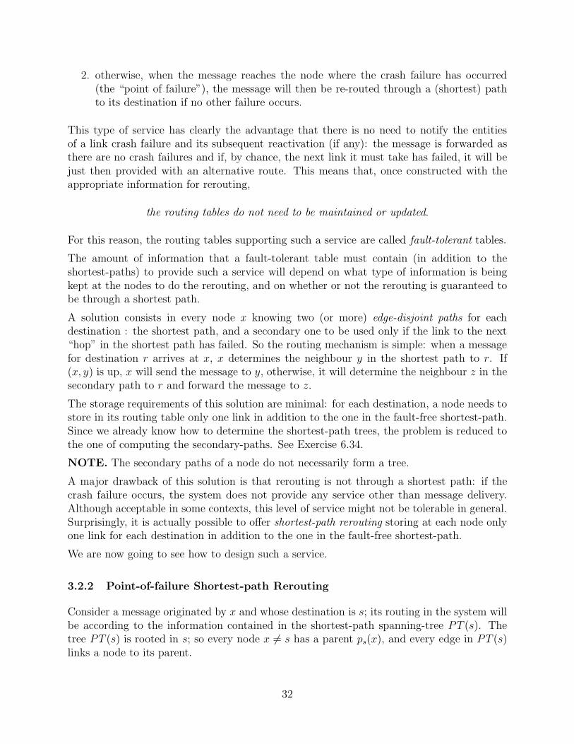
2. otherwise, when the message reaches the node where the crash failure has occurred(the “point of failure”), the message will then be re-routed through a (shortest) pathto its destination if no other failure occurs.

This type of service has clearly the advantage that there is no need to notify the entitiesof a link crash failure and its subsequent reactivation (if any): the message is forwarded asthere are no crash failures and if, by chance, the next link it must take has failed, it will bejust then provided with an alternative route. This means that, once constructed with theappropriate information for rerouting,

the routing tables do not need to be maintained or updated.

For this reason, the routing tables supporting such a service are called fault-tolerant tables.

The amount of information that a fault-tolerant table must contain (in addition to theshortest-paths) to provide such a service will depend on what type of information is beingkept at the nodes to do the rerouting, and on whether or not the rerouting is guaranteed tobe through a shortest path.

A solution consists in every node x knowing two (or more) edge-disjoint paths for eachdestination : the shortest path, and a secondary one to be used only if the link to the next“hop” in the shortest path has failed. So the routing mechanism is simple: when a messagefor destination r arrives at x, x determines the neighbour y in the shortest path to r. If(x, y) is up, x will send the message to y, otherwise, it will determine the neighbour z in thesecondary path to r and forward the message to z.

The storage requirements of this solution are minimal: for each destination, a node needs tostore in its routing table only one link in addition to the one in the fault-free shortest-path.Since we already know how to determine the shortest-path trees, the problem is reduced tothe one of computing the secondary-paths. See Exercise 6.34.

NOTE. The secondary paths of a node do not necessarily form a tree.

A major drawback of this solution is that rerouting is not through a shortest path: if thecrash failure occurs, the system does not provide any service other than message delivery.Although acceptable in some contexts, this level of service might not be tolerable in general.Surprisingly, it is actually possible to offer shortest-path rerouting storing at each node onlyone link for each destination in addition to the one in the fault-free shortest-path.

We are now going to see how to design such a service.

3.2.2 Point-of-failure Shortest-path Rerouting

Consider a message originated by x and whose destination is s; its routing in the system willbe according to the information contained in the shortest-path spanning-tree PT (s). Thetree PT (s) is rooted in s; so every node x 6= s has a parent ps(x), and every edge in PT (s)links a node to its parent.

32

When the link es[x] = (ps(x), x) fails, it disconnects the tree into two subtrees, one containings and the other x; call them T [s− x] and T [x− s]; see Figure 13.

p (x)s

s

x

T[x−s]T[s−x]

Figure 13: The crash failure of es[x] = (ps(x), x) disconnects the tree PT (s).

When ex fails, a new path from x to s must be found. It can not be any: it must be theshortest path possible between x and s in the network without es[x].

Consider a link e = (u, v) ∈ G \ PT (s), not part of the tree, that can reconnect the twosubtrees created by the crash failure of es[x]; i.e., u ∈ T [s−x] and v ∈ T [x− s]. We will callsuch a link a swap edge for es[x].

Using e we can create a new path from x to s: the path will consist of three parts: the pathfrom x to v in T [x/ex], the edge (u, v), and the path from u to s; see Figure 14. The cost ofgoing from x to s using this path will then be

dPT (s)(s, u) + θ(u, v) + dPT (s)(v, x) = d(s, u) + θ(u, v) + d(v, x)

This is the cost of using e as a swap for es[x]. For each es[x] there are several edges thatcan be used as swaps, each with a different cost. If we want to offer shortest-path reroutingfrom x to s when es[x] fails, we must use the optimal swap, that is the swap edge for es[x]of minimum cost.

So the first task that must be solved is to how find the optimal swap for each edge es[x] inPT (s). This computation can be done efficiently (Exercises 6.37 and 6.38); its result is thatevery node x knows the optimal swap edge for its incident link es[x]. To be used to constructthe PSR routing tables, this process must be repeated n times, one for each destination s(i.e., for each shortest-path spanning tree PT (s)).

Once the information about the optimal swap edges has been determined, it needs to beintegrated in the routing tables so to provide point-of-failure shortest-path rerouting.

The routing table of a node x must contain information about (1) the shortest paths as wellas about (2) the alternative paths using the optimal swaps:

33

u v

x

s

Figure 14: Point-of-failure rerouting using the swap edge e = (u, v) of es[x].

Final Normal Rerouting Swap SwapDestination Link Link Destination Link

s (ps(x), x) (pv(x), x) v (u, v)

Table 8: Entry in the routing table of x; e = (u, v) is the optimal swap edge for es[x].

1. Shortest path information. First and foremost, the routing table of x contains foreach destination s the link to the neighbour in the shortest path to s if there are nofailures. Denote by ps(x) this neighbour; the choice of symbol is not accidental: thisneighbour is the parent of x in PT (s) and the link is really es[x] = (ps(x), x).

2. Alternative path information. In the entry for the destination s, the routingtable of x must also contain the information needed to reroute the message if es[x] =(ps(x), x) is down. Let us see what this information is.

Let e = (u, v) be the optimal swap edge that x has computed for es[x]; this meansthat the shortest-path from x to s if es[x] fails is by first going from x to v, then overthe link (u, v), and finally from u to s. In other words, if es[x] fails, x must reroutethe message for s to v; i.e., x must send it to its neighbour in the shortest path tov. The shortest-paths to v are described by the tree PT (v); in fact, this neighbour isjust pv(x) and the link over which the message to s must be sent when rerouting isprecisely ev[x] = (pv(x), x) (see Exercise 6.39).

Concluding, the additional information x must keep in the entry for destination s arethe rerouting link ev[x] = (pv(x), x) and the closest node v on the optimal swap edgefor es[x]; this information will be used only if es[x] is down.

Any message must thus contain, in addition to the final destination (node s in our example),also a field indicating the swap destination (node v in our example), the swap link (link (u, v)

34

in our example) and a bit to explain which of the two must be considered (see Table 8). Therouting mechanism is rather simple. Consider a message originating from r for node s.

PSR routing mechanism

1. Initially, r sets the final destination to s, the swap destination and the swap link toempty, and the bit to 0; it then sends the message towards the final destination usingthe normal link indicated in its routing table.

2. If a node x receives the message with final destination s and bit set to 0, then

(a) if x = s the message has reached its destination: s processes the message.

(b) if es[x] = (ps(x), x) is up, x forwards the unchanged message on that link.

(c) if es[x] = (ps(x), x) is down, then x

i. copies to the swap destination and swap link fields of the message the swapdestination and swap link entries for s in its routing table;

ii. sets the bit to 1;

iii. sends the message on the rerouting link indicated in its table

3. If a node x receives the message with final destination s and bit set to 1, and swapdestination set to v, then

(a) if x = v then

i. it sets the bit to 0;

ii. it sends the message on the swap link.

(b) otherwise, it forwards the unchanged message on the link ev[x] = (pv(x), x).

Mode SwapDest SwapLink ContentDestination

1 v (u, v) INFOs

Figure 15: Message rerouted by x using the swap edge e = (u, v) of es[x].

3.3 On Correctness and Guarantees

3.3.1 Adaptive Routing

In all adaptive routing approaches, maintenance of the tables is carried out by broadcastinginformation about the status of the network; this can be done periodically or just when

35

changes do occur. In all cases, news of changes detected by a node will eventually reachany node (still connected to it). However, due to time delays, while an update is beingdisseminated, nodes still unaware will be routing messages based on incorrect information.In other words, as long as there are changes occurring in the system (and for some timeafterwards), the information in the tables is unreliable and might be incorrect. In particular,it is likely that routing will not be done through a shortest path; it is actually possible thatmessages might not be delivered as long as there are changes. This sad status of affairs isnot due to the individual solutions but solely to the fact that time delays are unpredictable.As a result,

it is impossible to make any guarantee on correctness and in particular on shortest-path delivery for adaptive routing mechanisms.

This situation occurs even if the changes at any time are few and their nature limited, as thesingle link crash failure (SLF). It would appear that we should be able to operate correctlyin such a system; unfortunately this is not true:

it is impossible to provide shortest-path routing even in the single link crash failure case

This is because the crash failure of a single edge can dramatically change all the shortest-path information; thus, when the link fails, every node must be notified so it can routemessages along the new shortest paths; the subsequent recovery of that node also will requiresuch a notification. Such an notification process needs to be repeated at each crash failureand recovery, and again the unpredictable time delays will make it impossible to guaranteecorrectness of the information available at the entities, and thus of the routing decision theymake based on that information.

Questions. What, if anything, can be guaranteed ?

The only think that we can say is that, if the changes stop (or there are no changes for along period of time) then the updates to the routing information converge to the correctstate, and routing will proceed according to the existing shortest paths. In other words, ifthe ”noise” caused by changes stops, eventually the entities get the correct result.

3.3.2 Fault-Tolerant Tables

In the fault-tolerant tables approach, no maintenance of the routing tables is needed oncethey have been constructed. Therefore, there are no broadcasts or notifications of changesthat, due to delays, might affect the correctness of the routing.

However, also faut-tolerant tables suffer because of the unpredictability of time delays. Forexample, even with the single link crash failure, point-of failure shortest-path rerouting cannot be guaranteed to be correct: while the message for s is being rerouted from x towardsthe swap edge es[x], the link es[x] might recover (i.e., come up again) and another link onthe may go down. Thus the message will again be rerouted, and might continue to do so ifa “bad” sequence of recovery-failure occurs. In other words, not only the message will not

36

reach s through a shortest-path from the first point-of-failure, but it will not reacg s at allas long as there is a change. It might be argued that such a sequence of events is highlyunlikely; but it is possible. Thus, again,

Questions. What, if anything, can be guaranteed ?

As in the case of adaptive routing, the only guarantee that if the changes stop (or thereare no changes for a long period of time) then messages will be (during that time) correctlydelivered through point-of-failure shortest paths.

4 Routing in Static Systems: Compact Tables

There are systems that are static in nature; for example, if Total Reliability holds, no changeswill occur in the network topology. We will consider static also any system where the routingtable, once constructed, can not be modified (e.g., because they are hardcoded/hardwired).Such is, for example, any system etched on a chip; should faults occur, the entire chip willbe replaced.

In these systems, an additional concern in the design of shortest-path routing tables is theirsize; that is, an additional design goal is to construct table that are as small as possible.

4.1 The Size of Routing Tables

The full routing table can be quite large. In fact, for each of its n−1 destinations, it containsthe specification (and the cost) of the shortest path to that destination. This means thateach entry possibly contains O(n logw) bits, where w ≥ n is the range of the entities’ names,for a total table size of O(n2 log w) bits. Assuming the best possible case, i.e., w = n, thenumber of bits required to store all the n full routing tables is

SFULL = O(n3 log n)

For n large, this is a formidable amount of space just to store the routing tables.

Observe that, for any destination, the first entry in the shortest path will always be a linkto a neighbour. Thus, it is possible to simplify the routing table by specifying for eachdestination y only the neighbour of x on the shortest path to it. Such a table is called short.For example, the short routing table for s in the network of Figure 1 is shown in Table 9.

In its short representation, each entry of the table of an entity x will contain log w bits torepresent the destination’s name and another log w bits, to represent the neighbour’s name.In other words, the table contains 2(n− 1) log w bits. Assuming the best possible case, i.e.,w = n , the number of bits required to store all the routing tables is

2n(n− 1) log n

This amount of space can be further reduced if, instead of the neighbours’ names we use thelocal port numbers leading to them. In this case, the size will be (n− 1)(log w + log px) bits,

37

Destination Neighbourh hk hc cd ce ef e

Table 9: Short representation of RT (s)

Port Destinationsports(h) h, kports(c) c, dports(e) e, f

Table 10: Alternative short representation of RT (s)

where px ≥ deg(x) is the range of the local port numbers of x. Assuming the best possiblecase, i.e., w = n and px = deg(x) for all x, this implies that the number of bits required tostore all the routing tables is at least

SSHORT =∑

x (n− 1) log deg(x) = (n− 1) log Πxdeg(x)

which can be still rather large.

Notice that the same information can be represented by listing for each port the destinationsreached via shortest-path through that port; e.g., see Table 10. This alternative representa-tion of RT (x) uses only deg(x) + (n− 1) log(n) bits for a total of

SALT =∑

x

(deg(x) + (n− 1) log n) = 2m + n(n− 1) log n (17)

It appears that there is not much more that it can be done to reduce the size of the table.This is however not the case if we, as designers of the system, had the power to choose thenames of the nodes and of the links.

4.2 Interval Routing

The question we are going to ask is whether it is possible to drastically reduce this amountof storage if we know the network topology and we have the power of choosing the names ofthe nodes and the port labels.

4.2.1 An Example: Ring Networks

Consider for example a ring network, and assume for the moment that all links have thesame cost.

38

2

1

3

4

5

6

5

0

7, 8, 0, 1

3, 4, 5, 6

left

right

right

(a) (b)

Figure 16: (a) Assigning names and labels. (b) Routing table of node 2

Suppose that we assign as names to the nodes consecutive integers, starting from 0 andcontinuing clockwise, and we label the ports right or left depending on whether or not theyare in the clockwise direction, respectively. See Figure 16(a).

Concentrate on node 0. This node, like all the others, has only two links. Thus, whenever 0has to route a message for z > 0, it must just decide whether to send it to right or to left.Observe that the choice will be right for 1 ≤ z ≤ ⌊n/2⌋, and left for ⌊n/2⌋+ 1 ≤ z ≤ n− 1.In other words, the destinations are consecutive integers (modulo n). This is true not justfor node 0: if x has to route a message for z 6= x, the choice will be right if z is in the interval< x + 1, x + 2, . . . x + ⌊n/2⌋ >, and left if z is in the interval < x + ⌊n/2⌋+ 1, . . . , x− 1 >,where the operations are modulo n. See Figure 16(b).

In other words, in all these routing tables, the set of destinations associated to a port is aninterval of consecutive integers, and, in each table, the intervals are disjoint. This is veryimportant for our purpose of reducing the space.

In fact, an interval has a very short representation: it is sufficient to store the two end values;that is just 2 log n bits. We can actually do it with just log n bits; see Exercise 6.40. Sincea table consists just of two intervals, we have routing tables of 4 log n bits each, for a grandtotal of just

4n log n

This amount should be contrasted with the one of Expression 17 that, in the case of ringsbecomes n2 log n + l.o.t.. In other words, we are able to go from quadratic to just linearspace requirements. Note that is is true even if the costs of the links are not all the same:Exercise 6.41.

The phenomenon we have just described is not isolated, as we will discuss next.

39

4.2.2 Routing with Intervals

Consider the names of the nodes in in a network G. Without any loss of generality, we canalways assume that the names are consecutive positive integers, starting from 0; that is, theset of names is Zn = 0, 1, . . . , n− 1.Given two integers j, k ∈ Zn, we denote by (j, k) the sequence

(j, k) = 〈j, j + 1, j + 2, . . . , k〉 if j < k(j, k) = 〈j, j + 1, j + 2, . . . n− 1, 0, 1, . . . , k〉 if j ≥ k

Such a sequence (j, k) is called a circular interval of Zn; the empty interval ∅ is also aninterval of Zn.

Suppose that we are able to assign names to the nodes so that the shortest-path routingtables for G have the following two properties. At every node x:

1. interval: For each link incident to x, the (names of the) destinations associated tothat link form a circular interval of Zn.

2. disjointness: Each destination is associated to only one link incident to x.

If this is the case, then we can have for G a very compact representation of the routing tables,like in the example of the ring network. In fact, for each link the set of destinations is aninterval of consecutive integers, and, like in the ring, the intervals associated to the links ofa given nodes are all disjoint.

In other words, each table consists of a set of intervals (some of them may be empty), onefor each incident link. From the storage point of view, this is very good news because wecan represent such intervals by just their start values (or, alternatively, by their end values).

In other words, the routing table of x will consist of just one entry for each of its links. Thismeans that the amount of storage for its table is only deg(x) log n bits. In turn, this meansthat the number of bits used in total to represent all the routing tables will be just

SINTERV AL =∑

x

deg(x) log n = 2 m log n (18)

How will the routing mechanism then work with such tables? Suppose x has a message whosedestination is y. Then x checks in its table which interval y is part of (since the intervalsare disjoint, y will belong to exactly one), and sends the message to the corresponding link.

Because of its nature, this approach is called interval routing. If it can be done, as wehave just seen, it allows for efficient shortest-path routing with a minimal amount of storagerequirements.

It however requires that we, as designers, find an appropriate way to assign names to nodesso that the interval and disjointness properties holds. Given a network G, it is not so obvioushow to do it or whether it can be done at all.

40

Tree Networks

First of all we will consider tree networks. As we will see, in a tree it is always possible toachieve our goal and can actually be done in several different ways.

Given a tree T , we first of all choose a node s as the source, transforming T into the treeT (s) rooted in s; in this tree, each node x has a parent and some children (possibly none).We then assign as names to the nodes consecutive integers, starting from 0, according to thepost-order traversal of T (s); e.g., using procedure

Post Order Naming(x, k)begin

Unnamed Children(x):= Children(x);while Unnamed Children(x) 6= ∅ do

y ← Unnamed Children(x);Post Order Naming(y, k)

endwhilemyname:= k;k:= k + 1;

end

started by calling Post Order Naming(s, 0). This assignment of names has several properties.For example, any node has a larger name than all its descendents. More importantly, it hasthe interval and disjointness properties (Exercise 6.45).

15

3 8 14

2 6 7 9 13

0 1 4 5 11 1210

Figure 17: Naming for interval routing in trees

Informally, the interval property follows is because, when executing Post Order Naming withinput (x, k), x and its descendents will be given as names consecutive integers starting fromk. See for example Figure 18.

41

8

< 7 >< 4, 5, 6 >

< 9, 10, 11, 12, 13, 14, 15, 0, 1, 2, 3 >

Figure 18: Disjoint intervals

Other Networks

Most regular network topologies we have considered in the past can be assigned namesso that interval routing is possible. This is for example the case of the p × q mesh andtorus, hypercube, butterfly, and cube-connected-cycles; see Exercises 6.48 and 6.49. For thesenetworks the construction is rather simple.

Using a more complex construction, names can be assigned so that interval routing can bedone also in any outerplanar graph (Exercise 6.50); recall that a graph is outerplanar if itcan be drawn in the plane with all the nodes lying on a ring and all edges lying in the interiorof the ring without crossings.

Question: Can interval routing be done in every network ?

The answer is unfortunately: No. In fact there exist rather simple networks, the so calledglobe graphs (one is shown in Figure 19), for which interval routing is impossible (Exercise6.52).

Figure 19: A globe graph: interval routing is not possible.

5 Bibliographical Notes

[12, 14, 15]

42

Shortest-paths: The O(n3) construction for a single tree was obtained independently by BobGallager [15] and To-Yat Cheung [9]. Chandi and J. Misra [19], C.C. Chen [8], T.Y. Cheung[9], J. Park and N. Tokura and T. Masuzawa and K. Hagihara [24], B. Awerbuch [2]

Long Messages (Exercise 6.15): Haldar [16]

Planar networks: Greg N. Frederickson [12]

BFS:Protocol BF (known as the “Coordinated Minimum Hop Algorithm”) is due to Bob Gallager[15]. Also to Gallager [15] is due the idea of reducing time by partitioning the layers ofthe breadth-first tree into groups (Section 2.4.3) and a series of time-messages tradeoffs (“Modified Coordinated Minimum Hop Algorithm”). Protocol BF Layers has been designedby Greg N. Frederickson [12]. The problem of reducing time while mantaining a reasonablemessage complexity has been investigated by B. Awerbuch [3], B. Awerbuch and R. G.Gallager [6], Zhu and T. Cheung [27]. The near-optimal bounds (Exercise 6.23) have beenobtained by B. Awerbuch [4].cover: B. Awerbuch and B. Berger and L. Cowen and D. Peleg [5]

Center-based and median-based routing was first dicussed in details by David W. Wall andSusanna Owicki [26]. The lower-bound on average edge-stretch and the construction ofspanning trees with low average edge-stretch (Exercises 6.31,6.32 and 6.33) are due to NogaAlon, Richard Karp, David Peleg and Doug West [1].

Edge-disjoint: Mohanty and Bhattacharjee [21]Storing, in addition to the shortest-path routing tables, k other spanning trees for eachdestination suggested by Alon Itai and M. Rodeh[17].Swap-edges: H. Ito and K. Iwama and Y. Okabe and T. Yoshihiro [18]. Enrico Nardelli,Guido Proietti and Peter Widmayer[23]. Paola Flocchini, Linda Pagli, Tony Mesa, GiuseppePrencipe, and Nicola Santoro [11].

Compact: Nicola Santoro and Ramez Kathib [25], Jan van Leeuwen and Richard Tan [20].Outerplanar graphs (Exercise 6.50) is due to Greg Frederickson and Ravi Janardan[13].Linear interval routing [7] by E.M. Bakker and Jan van Leeuwen and Richard Tan (Exercise6.51 and Problem 6.1)Characterization Lata Narayanan and Sunil Shende [22] and T. Eilam and Shlomo Moranand Shmuel Zaks [10].

6 Exercises, Problems, and Answers

6.1 Exercises

Exercise 6.1 Write the set of rules corresponding to Protocol Map Gossip described in Sec-tion 2.1.

43

Exercise 6.2 ⋆ ⋆ ⋆Consider a tree network where each entity has a single item of information. Determine thetime costs of gossiping. What would the time costs be if each entity x initially has deg(x)items ?

Exercise 6.3 Consider a tree network where each entity has f(n) items of information.Assume that messages can contain g(n) items of information (instead of O(1)); with howmany messages can gossiping be performed ?

Exercise 6.4 Using your answer to question 6.3, with how many messages can all routingtable be constructed if g(n) = O(n)?

Exercise 6.5 Consider a tree network where each entity has f(n) items of information.Assume that messages can contain g(n) items of information (instead of O(1)); with howmany messages can all items of information be collected at a single entity ?

Exercise 6.6 Using your answer to question 6.5, with how many messages can all routingtable be constructed at that single entity if g(n) = O(n)?

Exercise 6.7 Write the set of rules corresponding to Protocol Iterated Construction de-scribed in Section 2.2. Implement and properly test your implementation.

Exercise 6.8 Prove that Protocol Iterated Construction converges to the correct routingtables, and will do so after at most n− 1 iterations. Hint. Use induction to prove that V i

x [z]is the cost of the shortest-path from x to z using at most i hops.

Exercise 6.9 We have assumed that the cost of a link is the same in both directions; i.e.,θ(x, y) = θ(y, x). However, there are cases when θ(x, y) can be different from θ(y, x). Whatmodifications have to be made so that Protocol Iterated Construction works correctly also inthose cases ?

Exercise 6.10 In protocol PT Construction, no action is provided for an idle entity re-ceiving an Expand message. Prove that such a message will never be received in such astate.

Exercise 6.11 In procedure Compute Local Minimum of protocol PT Construction, an en-tity might set path length to infinity. Show that, if this happens, this entity will set path lengthto infinity in all subsequent iterations.

Exercise 6.12 In protocol PT Construction, each entity will eventually set path length toinfinity. Show that, when this happens to a leaf of the constructed tree, that entity can beremoved from further computations.

Exercise 6.13 Modify protocol PT Construction so it constructs the routing table RT (s) ofthe source s.

44

Exercise 6.14 We have assumed that the cost of a link is the same in both directions; i.e.,θ(x, y) = θ(y, x). However, there are cases when θ(x, y) can be different from θ(y, x). Whatmodifications have to be made so that Protocol PT Construction works correctly also in thosecases ?

Exercise 6.15 Assume that messages can contain O(n) items of information (instead ofO(1)). Show how to construct all the shortest-path trees with just O(n2) messages.

Exercise 6.16 Prove that, after iteration i− 1 of Protocol BF Construction,(a) all the nodes at distance up to i− 1 are part of the tree;(c) each node at distance i− 1 knows which of its neighbours are at distance i− 1.

Exercise 6.17 Write the set of rules corresponding to Protocol BF described in Section 2.2.Implement and properly test your implementation.

Exercise 6.18 Write the set of rules corresponding to Protocol BF Levels. Implement andproperly test your implementation.

Exercise 6.19 Let Explore(j, k) be the first message x accepts in the expansion phase ofprotocol BF Levels. Prove that the number of times x will change its level in this phase is atmost j − t + 1 < l.

Exercise 6.20 Prove that, in the expansion phase of an iteration of Protocol BF Levels, allnodes in levels t + 1 to t + l are reached and attached to the existing fragment, where t is thelevel of the sources (i.e., the leaves in the current fragment).

Exercise 6.21 Consider protocol BF Levels when l = d(G). Show how to obtain the samemessage and time complexity without any a priori knowledge of d(G).

Exercise 6.22 Prove that, if we choose l = d(G) in protocol BF Levels, then in any syn-chronous execution the number of messages will be exactly 2m + n− 1.

Exercise 6.23 ⋆⋆Show how to construct a breadth-first spanning-tree in time O(d(G)1+ǫ) using no more thanO(m1+ǫ) messages, for any ǫ > 0.

Exercise 6.24 Let c be a center of G and let SPT (c) be the shortest-path tree of c. Provethat diam(G) = diam(SPT (c)).

Exercise 6.25 Let T be a spanning-tree of G. Prove that∑

(x,y)∈T |T [x−y]||T [y−x]|w(x, y) =∑

u,v∈T dT (u, v).

Exercise 6.26 (median-based routing)Let z be a median of G (i.e., a node for which the sum of distances to all other nodes isminimized) and let PT (z) be the shortest-path tree of z. Prove that Traffic(PT (z)) ≤ 2Traffic(T⋆), where T⋆ is the spanning-tree of G for which Traffic is minimized.

45

Exercise 6.27 Consider a ring network Rn with weighted edges. Prove or disprove thatPT (c) = MSP (Rn), where c is a center of Rn and MSP (Rn) is the minimum-cost spanning-tree of Rn.

Exercise 6.28 Consider a ring network Rn with weighted edges. Let c and z be a centerand a median of Rn, respectively.

1. For each of the following spanning trees of Rn, compare the stretch factor and theedge-stretch factor: PT (c), PT (z), and the minimum-cost spanning-tree MSP (Rn).

2. Determine bounds on the average edge-stretch factor of PT (c), PT (z), and MSP (Rn).

Exercise 6.29 ⋆Consider a a× a square mesh Ma,a where all costs are the same.

1. Is it possible to construct two spanning-trees T ′ and T ′′ such that σ(T ′) < σ(T ′′) butǫ(T ′) > ǫ(T ′′) ? Explain.

2. Is it possible to construct two spanning-trees T ′ and T ′′ such that σ(T ′) < σ(T ′′) butǫ(T ′) > ǫ(T ′′) ? Explain.

Exercise 6.30 Consider a square mesh Ma,a where all costs are the same. Construct twospanning-trees T ′ and T ′′ such that σ(T ′) < σ(T ′′) but ǫ(T ′) > ǫ(T ′′).

Exercise 6.31 ⋆Show that there are graphs G with unweighted edges where ǫG(T ) = Ω(log n) for every span-ning tree T of G

Exercise 6.32 ⋆⋆Design an efficient protocol for computing a spanning tree with low average edge-stretch of anetwork G with unweighted edges.

Exercise 6.33 ⋆⋆Design an efficient protocol for computing a spanning tree with low average edge-stretch of anetwork G with weighted edges.

Exercise 6.34 ⋆Design a protocol for computing the secondary-paths of a node x. You may assume that theshortest path tree PT (x) has already been constructed and that each node knows its and itsneighbours’ distance from x. Your protocol should use no more messages than that requiredto construct PT (x).

Exercise 6.35 (split horizon) ⋆⋆Consider the following technique, called split horizon, for solving the count-to-infinity prob-lem discussed in Section 3.1.2: during an iteration, a node a does not send its cost fordestination c to its neighbour b if b is the next node in the “best” path (so far) from a to c.In the example of Figure 12, in the first iteration y does not send its cost for w to z, andthus z will correctly set its cost for w to K. In the next two iterations y and x will correctlyset their cost for w to K + 1 and K + 2, respectively. Prove or disprove that split horizonsolves the count-to-infinity problem.

46

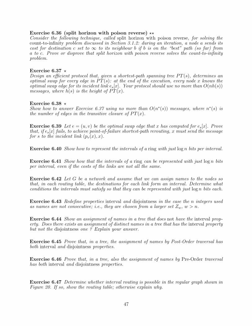
Exercise 6.36 (split horizon with poison reverse) ⋆⋆Consider the following technique, called split horizon with poison reverse, for solving thecount-to-infinity problem discussed in Section 3.1.2: during an iteration, a node a sends itscost for destination c set to ∞ to its neighbour b if b is on the “best” path (so far) froma to c. Prove or disprove that split horizon with poison reverse solves the count-to-infinityproblem.

Exercise 6.37 ⋆Design an efficient protocol that, given a shortest-path spanning tree PT (s), determines anoptimal swap for every edge in PT (s): at the end of the execution, every node x knows theoptimal swap edge for its incident link es[x]. Your protocol should use no more than O(nh(s))messages, where h(s) is the height of PT (x).

Exercise 6.38 ⋆Show how to answer Exercise 6.37 using no more than O(n∗(s)) messages, where n∗(s) isthe number of edges in the transitive closure of PT (x).

Exercise 6.39 Let e = (u, v) be the optimal swap edge that x has computed for es[x]. Provethat, if es[x] fails, to achieve point-of-failure shortest-path rerouting, x must send the messagefor s to the incident link (pv(x), x).

Exercise 6.40 Show how to represent the intervals of a ring with just log n bits per interval.

Exercise 6.41 Show how that the intervals of a ring can be represented with just log n bitsper interval, even if the costs of the links are not all the same.

Exercise 6.42 Let G be a network and assume that we can assign names to the nodes sothat, in each routing table, the destinations for each link form an interval. Determine whatconditions the intervals must satisfy so that they can be represented with just log n bits each.

Exercise 6.43 Redefine properties interval and disjointness in the case the n integers usedas names are not consecutive; i.e., they are chosen from a larger set Zw, w > n.

Exercise 6.44 Show an assignment of names in a tree that does not have the interval prop-erty. Does there exists an assignment of distinct names in a tree that has the interval propertybut not the disjointness one ? Explain your answer.

Exercise 6.45 Prove that, in a tree, the assignment of names by Post-Order traversal hasboth interval and disjointness properties.

Exercise 6.46 Prove that, in a tree, also the assignment of names by Pre-Order traversalhas both interval and disjointness properties.

Exercise 6.47 Determine whether interval routing is possible in the regular graph shown inFigure 20. If so, show the routing table; otherwise explain why.

47

taaaaa

t

t

t t

t t

t

t

t

t

t t

t

t

bb

bb

bb

bb

@@

@@@

@@

@@

@@

@@

t

@@

@@

Figure 20: A regular graph.

Exercise 6.48 Design an optimal interval routing scheme for p × q mesh and torus. Howmany bits of storage will it require ?

Exercise 6.49 Design an optimal interval routing scheme for a d-dimensional(a) hypercube; (b) butterfly; (c) cube-connected cycles. How many bits of total storage willeach require ?

Exercise 6.50 ⋆⋆ Show how to assign names to the nodes of an outerplanar graph so thatinterval routing is possible.

Exercise 6.51 ⋆⋆ If for every x all the intervals in its routing table are strictly increasing(i.e., there is no “wraparound” node ”0), the interval routing is called linear. Prove that thereare networks for which there exists interval routing but linear interval routing is impossible.

Exercise 6.52 Prove that in the globe graph of Figure 19 interval routing is not possible.

6.2 Problems

Problem 6.1 Linear Interval Routing. ⋆⋆ If for every x all the intervals in its routingtable are strictly increasing (i.e., there is no “wraparound” node ”0), the interval routing iscalled linear. Characterize the class of graphs for which there exists a linear interval routing.

48

Figure 21: Graph with interval routing but where no linear interval routing exists.

6.3 Answers to Exercises

Partial Answer to Exercise 6.23.Choose the size of the strip to be k =

√

d(G). A strip cover is a collection of trees thatspan all the source nodes of a strip. In iteration i, first of all construct a “good” cover of strip i

Answer to Exercise 6.26.Observe that, for any spanning tree T of G, Traffic(T ) =

∑

u,v∈V dT (u, v) (Exercise 6.25). LetSumDist(x) =

∑

u∈V dG(u, x); clearly Traffic(T⋆) ≥∑

x∈V SumDist(x). Let z be a medianof G (i.e., a node for which SumDist is minimized); then SumDist(z) ≤ 1

nTraffic(T⋆).

Thus we have that Traffic(PT (z)) =∑

u,v∈V dPT (z)(u, v) ≤∑

u,v∈V (dPT (z)(u, z)+dPT (z)(z, v))≤ (n−1)

∑

u∈V (dPT (z)(u, z)+(n−1)∑

v∈V (dPT (z)(v, z) = 2(n−1)SumDist(z) ≤ 2Traffic(T⋆).

Answer to Exercise 6.40.In the table of node x, the interval associated to right always starts with x+1 while the oneassociate to left always ends with x− 1. Hence, for each interval, it is sufficient to store onlythe other end value.

Partial Answer to Exercise 6.51.Consider the graph shown in Figure 21.

References

[1] Noga Alon, Richard M. Karp, David Peleg, and Douglas West. A graph-theoretic gameand its application to the k-server problem. SIAM Journal of Computing, 24:78–100,1995.

[2] Baruch Awerbuch. Complexity of network synchronization. Journal of the ACM,32(4):804–823, October 1985.

49

[3] Baruch Awerbuch. Reducing complexities of the distributed max-flow and breadth-first-search algorithms by means of network synchronization. Networks, 15:425–437,1985.

[4] Baruch Awerbuch. Distributed shortest path algorithms. In Proc. 21st Ann. ACMSymp. on Theory of Computing, pages 490–500, 1989.

[5] Baruch Awerbuch, B. Berger, L. Cowen, and David Peleg. Near-linear cost sequentialand distributed constructions of sparse neighborhood covers. In Proceedings. 34th An-nual Symposium on Foundations of Computer Science, pages 638–647, New York, 3-5Nov. 1993.

[6] Baruch Awerbuch and Robert G. Gallager. A new distributed algorithm to find breadthfirst search trees. IEEE Transactions on Information Theory, 33:315–322, 1987.

[7] E.M. Bakker, Jan van Leeuwen, and Richard Tan. Linear interval routing. AlgorithmsReview, 2(2):45–61, 1991.

[8] C.C. Chen. A distributed algorithm for shortest paths. IEEE Transactions on Com-puters, C-31:898–899, 1982.

[9] To-Yat Cheung. Graph traversal techniques and the maximum flow problem in dis-tributed computation. IEEE Transactions on Software Engineering, 9:504–512, 1983.

[10] T. Eilam, Shlomo Moran, and Shmuel Zaks. The complexity of the characterization ofnetworks supporting shortest-path interval routing. In 4th International Colloquium onStructural Information and Communication Complexity, pages 99–11, Ascona, 1997.

[11] Paola Flocchini, Linda Pagli, Tony Mesa, Giuseppe Prencipe, and Nicola Santoro. Anefficient protocol for computing the optimal swap edges of a shortest path tree. In ??,2004.

[12] Greg N. Frederickson. A distributed shortest path algorithm for a planar network.Information and Computation, 86(2):140–159, June 1990.

[13] Greg N. Frederickson and Ravi Janardan. Designing networks with compact routingtables. Algorithmica, 3:171–190, June 1988.

[14] Eli Gafni and D.P. Bertsekas. Distributed algorithms for generating loop-free routes innetworks with frequently changing topology. IEEE Transactions on Communication,Com-29:11–18, January 1981.

[15] Robert G. Gallager. Distributed minimum hop algorithms. Technical Report LIDS-P-1175, Laboratory for Information and Decision Systems, Massachusetts Institute ofTechnology, 1982.

[16] S. Haldar. An ‘all pairs shortest paths’ distributed algorithm using 2n2 messages. InProceedings of the 19th International Workshop on Graph-Theoretic Concepts in Com-puter Science (WG’93), Utrecht, Netherlands, June 1993.

50

[17] Alon Itai and M. Rodeh. The multi-tree approach to reliability in distributed networks.Information and Computation, 79:43–59, 1988.

[18] H. Ito, K. Iwama, Y. Okabe, and T. Yoshihiro. Polynomial-time computable backuptables for shortest-path routing. In Proc. of 10th Colloquium on Structural Informationand Communication Complexity (SIROCCO 2003), pages 163–177, 2003.

[19] J. Misra K.M. Chandi. Distributed computations on graphs: shortest path algorithms.Communications of ACM, 25(11):833–837, November 1982.

[20] Jan van Leeuwen and Richard B. Tan. Interval routing. The Computer Journal, 30:298–307, 1987.

[21] H. Mohanty and G.P.Bhattacharjee. A distributed algorithm for edge-disjoint pathproblem. In 6th Conference on Foundations of Software Technology and TheoreticalComputer Science (FSTTCS), volume 241 of Lecture Notes in Computer Science, pages344–361, New Delhi, 1986. Springer.

[22] Lata Narayanan and Sunil Shende. Characterization of networks supporting shortest-path interval labelling schemes. In 3rd International Colloquium on Structural Infor-mation and Communication Complexity, pages 73–87, 1996.

[23] Enrico Nardelli, Guido Proietti, and Peter Widmayer. Swapping a failing edge of asingle source shortest paths tree is good and fast. Algoritmica, 35:56–74, 2003.

[24] J. Park, N. Tokura, T. Masuzawa, and K. Hagihara. An efficient distributed algorithmfor constructing a breadth-first search tree. Systems and Computers in Japan, 20:15–30,1989.

[25] Nicola Santoro and Ramez Khatib. Labeling and implicit routing in networks. TheComputer Journal, 28:5–8, 1985.

[26] David W. Wall and Susanna Owicki. Construction of centered shortest-path trees innetworks. Networks, 13(2):207–332, 1983.

[27] Y. Zhu and To-Yat Cheung. A new distributed breadth-first-search algorithm. Infor-mation Processing Letters, 25:329–333, 1987.

51