
Chapter 4 - Princeton University Press
48
COPYRIGHT NOTICE: Matthew O. Jackson: Social and Economic Networks is published by Princeton University Press and copyrighted, © 2008, by Princeton University Press. All rights reserved. No part of this book may be reproduced in any form by any electronic or mechanical means (including photocopying, recording, or information storage and retrieval) without permission in writing from the publisher, except for reading and browsing via the World Wide Web. Users are not permitted to mount this file on any network servers. Follow links for Class Use and other Permissions. For more information send email to: [email protected]
Transcript of Chapter 4 - Princeton University Press

COPYRIGHT NOTICE:
Matthew O. Jackson: Social and Economic Networks is published by Princeton University Press and copyrighted, © 2008, by Princeton University Press. All rights reserved. No part of this book may be reproduced in any form by any electronic or mechanical means (including photocopying, recording, or information storage and retrieval) without permission in writing from the publisher, except for reading and browsing via the World Wide Web. Users are not permitted to mount this file on any network servers.
Follow links for Class Use and other Permissions. For more information send email to: [email protected]
CHAPTER 4Random-Graph Models of Networks
In this chapter, I discuss a few of the workhorse models of static random networks and some of the properties that they exhibit. As we saw in Chapter 1, randomly generated networks exhibit a variety of features found in the data, and through examining the properties of these models we can begin to trace traits of observed networks to characteristics of the formation process.
Models of random networks find their origin in the studies of random graphs by Solomonoff and Rapoport [611], Rapoport [553], and Erd¨ enyi [227], os and R´[228], [229]. The canonical version of such a model, a Poisson random graph, was discussed in Section 1.2.3. The next chapter is a “sister” to this one, in which I discuss a series of recent models of growing random networks that attempt to match more of the properties, such as those discussed in Chapter 3, that are exhibited by many observed networks. Indeed, random-graph models of networks have been a primary tool in analyzing various observed networks. For example the network of high school romances described in Section 1.2.2 has several features that are well described by a random-network model, such as a single giant component, a large number of much smaller components, and a few isolated nodes. Such random models of network formation help tie observed social patterns to the structure of the inherent randomness and the process of link formation.
Beyond their direct use in analyzing observed networks, random-network models also serve as a platform for modeling how behaviors diffuse through a network. For instance, the spread of a disease depends on the contacts among various individuals. That spread can be very different, depending on the average amount of interaction (e.g., interactions with a few others, or with hundreds of others) and its distribution in the population (e.g., everyone interacts with roughly the same number of people, or some people have contact with large numbers while others have contact with few). To understand how such diffusion works, one has to have a tractable model of the link structure within a society, and random-graph models provide such a base. These models are not only useful in understanding the diffusion of a disease, but also in modeling phenomena like the spread of information
77

78 Chapter 4 Random-Graph Models of Networks
or decisions that are heavily influenced by peers (e.g., whether to go to college), as we shall see in more detail in Chapters 7 and 8.
Let me reiterate that random models of network formation are largely context-free, in that the nodes and processes for link formation are often simply governed by some given probabilistic rules. Some of these probabilistic rules have stories behind them, but this is not true of all such models. Thus these models are generally missing the social and economic incentives and pressures that underlie network formation, as discussed more fully in Chapter 6. Nevertheless, these models are still quite useful for the reasons mentioned above, and they also serve as benchmarks. By keeping track of the properties that random-graph models of networks exhibit, and which ones they fail to exhibit, we develop a reference point for building richer models and understanding the strengths and weaknesses of models that are tied to social and economic forces influencing individual decisions to form and maintain relationships.
The chapter starts with the presentation of a series of fundamental random-graph models that have been useful in various aspects of network analysis. They include variations on the basic Poisson random-graph model with correlations between links and allow richer degree distributions to be generated. I then present some properties of the resulting networks. These include understanding how small changes in underlying parameters can lead to large changes in the properties of the resulting graphs (thresholds and phase transitions), as well as understanding the conditions for connectedness and existence of a giant component, and other properties, such as diameter and clustering. The chapter concludes with an illustration of how random networks can be used as a basis for understanding the spread of contagious diseases or behaviors in a society.
4.1 Static Random-Graph Models of Random Networks
The term static refers to a typed model in which all nodes are established at the same time and then links are drawn between them according to some probabilistic rule. Poisson random graphs constitute one such static model. This class of static models contrasts with processes where networks grow over time. In the latter type of models new nodes are introduced over time and form links with existing nodes as they enter the network. Such growing processes can result in properties that are different from those of static networks, and they allow different tools for analysis. They are also naturally suited to different applications and are discussed in detail in Chapter 5.
4.1.1 Poisson and Related Random-Network Models
The Poisson random-graph model is one of the most extensively studied models in the static family. Closely related models are the ones mentioned in footnote 9 in Section 1.2.3, in which a network is randomly chosen from some set of networks. For instance, out of all possible networks on n nodes, one could simply pick one completely at random, with each network having an equal probability of being chosen. Alternatively, one could simply specify that the network should have M

√
79 4.1 Static Random-Graph Models of Random Networks
links, and then pick one of those networks at random with equal probability (i.e., (N
)−1 ( n )
with each M link network having probability M
, where N = 2 is the number of potential links among n nodes). Some of these models of random networks have remarkably similar properties. On an intuitive level, if in a network each link is formed with independent probability p, we expect to have pn(n − 1)/2 links formed, where n(n − 1)/2 is the potential number of links. While we might end up with more or fewer links, for a large number of nodes, an application of the law of large numbers ensures that the final number of links will not deviate too much from this expected number in terms of the percentage formed. This result guarantees that a model in which links are formed independently has many properties in common with a model network that is prescribed to have the expected number of links.1
While these networks are static in the way they are generated, much of the analysis of such random networks concerns what happens when n becomes large. It is easy to understand why most results for random graphs are stated for large numbers of nodes. For example, in the Poisson random-graph model, if we fix the number of nodes and some probability of a link forming, then every conceivable network has some positive probability of appearing. To talk sensibly about what might emerge, we want to make statements of the sort that networks exhibiting some property are (much) more likely to appear than networks that fail to exhibit that property. Thus most results in random-graph theory concern the probability that a network generated by one of these processes has a given property as n goes to infinity. For instance, what is the probability that a network will be connected, and how does this depend on how p behaves as a function of n? Many such results are proven by finding some lower or upper bound on the probability that a given property holds and then determining whether the bounds can be shown to converge to 0 or 1 as n becomes large. We shall examine some of these properties for a general class of static random networks later in the chapter.
Let me begin, however, by describing some variations of static random-graph models other than the Poisson model that provide a feel for the variety of such models and the motivations behind their development.
4.1.2 Small-World Networks
While random graphs can exhibit some features of observed social networks (e.g., diameters that are small relative to the size of the network when the average degree grows sufficiently quickly), it is clear that random graphs lack certain features that are prevalent among social networks, such as the high clustering discussed in Sections 3.2.2 and 3.2.5. To see this, consider the Poisson random-network model,
1. Let G(n, p) denote the Poisson random-graph model on n nodes with probability p of any given link, and G(n, M) denote the model network with M links chosen with a uniform probability over all networks of M links on n nodes. The properties of G(n, p) and G(n, M) are closely related for large n when M is near pn(n − 1)/2. In particular, if n 2p(1 − p) → ∞, and a property holds for each sequence of Ms that lie within p(1 − p)n of pn(n − 1)/2, then it holds for G(n, p). The converse holds for a rich class of properties (called convex properties). See Chapter 2 in Bollobas [86] for detailed definitions and results.

80 Chapter 4 Random-Graph Models of Networks
23 22
21
20
19
18
17
2425
1
2
3
4
5
6
7
8 9
10 11 12 13
14
15
16
FIGURE 4.1 A ring lattice on 25 nodes with 50 links.
and let us ask what its clustering is. Suppose that i and j are linked and j and k are linked. What is the frequency with which i and k will be linked? Since link formation is completely independent, it is simply p. Thus, as n becomes large, if the average degree grows more slowly than n (which would be true in most large social and economic networks in which there are some bounds on the number of links that agents can maintain) then it must be that p tends to 0 and so the clustering (both average and overall) also tends to 0.
With this tendency in mind, Watts and Strogatz [658] developed a variation of a random network showing that only a small number of randomly placed links in a network are needed to generate a small diameter. They combined this model with a highly regular and clustered starting network to generate networks that simultaneously exhibit high clustering and low diameter, a combination observed in many social networks. Their point is easy to see. Suppose we start with a very structured network that exhibits a high degree of clustering. For instance, construct a large circle but connect a given node to the nearest four nodes rather than just its nearest two neighbors, as in Figure 4.1.
In such a network, each node’s individual clustering coefficient is 1/2. To see this, consider some sequence of consecutive nodes 1, 2, 3, 4, 5, that are part of the network for a large n. Consider node 3, which is connected to each of nodes 1, 2, 4, and 5. Out of all the pairs of 3’s neighbors ({1, 2}, {1, 4}, {1, 5}, {2, 4}, {2, 5}, {4, 5}), half of them are connected: ({1, 2}, {2, 4}, {4, 5}). As n grows, the clustering (both overall and average) stays constant at 1/2. By adjusting the structure of the local connections, we can also adjust the clustering.
While this sort of regular network exhibits high clustering, it fails to exhibit some of the other features of many observed networks, such as a small diameteter and at least some variance in the degree distribution. The diameter of such a network is on the order of n/4. The main point of Watts and Strogatz [658] is that by randomly rewiring relatively few links, we can create a network that has a much smaller diameter but still exhibits substantial clustering. The rewiring can be

81 4.1 Static Random-Graph Models of Random Networks
23 24
22
21
20
19
18
251
2
3
4
5
6
7
8
9 10
11 12 13 14
15
16
17
FIGURE 4.2 A ring lattice on 25 nodes starting with 50 links and rewiring seven of them.
done by randomly selecting some link ij and disconnecting it, and then randomly connecting i to another node k chosen uniformly at random from nodes that are not already neighbors of i. Of course, as more such rewiring is done, the clustering will eventually vanish. The interesting region is where enough rewiring has been done to substantially reduce (average and maximal) path length, but not so much that clustering vanishes.
After having rewired just six links, the diameter of the network has decreased from 6 in the network pictured in Figure 4.1 to 5 in the one shown in Figure 4.2, with minimal impact on the clustering. Note also that in Figure 4.1, every node is at distance 6 from three other nodes (e.g., node 1 and nodes 13, 14, and 15), so the rewiring has not simply shortened a few long paths, but rather these new links shorten many paths in the network: there are 39 pairs of nodes at a distance of 6 from each other in the original network that are all moved closer by the rewiring. This example is suggestive, and Watts and Strogatz perform simulations to provide an idea of how the process behaves for ranges of parameters.
This model makes an interesting point in showing how clustering can be maintained in the presence of enough random link formation to produce a low diameter. The model also has obvious shortcomings; in particular, the degree distribution is essentially a convex combination of a degenerate distribution with all weight on a single degree and a Poisson distribution. Such a degree distribution is fairly specific to this model and not often observed in social networks. I discuss alternative models that better match observed degree distributions in Section 5.3.
4.1.3 Markov Graphs and p* Networks
In this section I describe a generalization of Poisson random graphs that has been useful in statistical analysis of observed networks and was introduced by Frank and Strauss [254]. They called this class of graphs Markov graphs.Such random-graph models were later imported to the social network literature by Wasserman and

82 Chapter 4 Random-Graph Models of Networks
Pattison [651] under the name of p ∗ networks, and further studied and extended.2
The basic motivation is to provide a model that can be statistically estimated and still allows for specific dependencies between the probabilities with which different links form.
Again, one important aspect of introducing dependencies is related to clustering, since Poisson random networks with average degrees growing more slowly than the number of nodes have clustering ratios tending to 0, which are too low to match many observed networks. Having dependencies in the model can produce nontrivial clustering.
Conditional dependencies can be introduced so that the probability of a link ik depends on whether ij and jk are present. The obvious challenge is that such dependencies tend to interact with one another in ways that could make it impossible to specify the probability of different graphs in a tractable manner. For instance, if the conditional probability of a link ik depends on whether ij and jk are present but also on whether any other adjacent pairs are present, and the conditional probability of jk depends on other adjacent pairs being present, and so on, we end up with a complicated set of dependencies. The important contribution of Frank and Strauss [254] is to make use of a theorem by Hammersley and Clifford (see Besag [60]) to derive a simple log-linear expression for the probability of any given network in the presence of arbitrary dependencies.
One of the more useful results of Frank and Strauss [254] can be expressed as follows. Consider n nodes, and keep track of the dependencies between links by another graph, D, which is a graph among all of the n(n − 1)/2 possible links.3
So D is not a graph on the original nodes but one whose nodes are all the possible links. The idea is that if ij and jk are neighbors in D, then there is some sort of conditional dependency between them, possibly in combination with other links. Thus D captures which links are dependent on which others, possibly in quite complicated combinations. For example, D is empty for the Poisson random-graph model, as all links are independent. If instead we wish to capture the idea that there might be clustering, then the link ik should depend on the presence of ij and kj for each possible j . Thus D would have ik connected to every other link that contains either i or k (and possibly others, depending on the other dependencies).
Let C(D) be all the cliques of D; that is, all of the completely connected subgraphs of D (where the singleton nodes are considered to be connected subgraphs). In the case of a Poisson random graph, C(D) is simply the set of all links ij . With some dependencies, the set C(D) includes all individual links and other cliques as well, for instance, all triads (sets of the form {ij, jk, ik}). Given a generic element A ∈ C(D), let IA(g) = 1 if A ⊂ g (viewing g as a set of links), and IA(g) = 0 otherwise. So if A is a triad {ij, jk, ik}, then IA(g) = 1 if each of the links ij , jk, and ik are in g, and IA(g) = 0 otherwise. Then Frank and Strauss use Hammersley and Clifford’s theorem to show that the probability of a given network g depends only on which cliques of D it contains:
2. For instance, see Pattison and Wasserman [534] for an extension to multiple interdependent networks on a common set of nodes. 3. This method is easily adapted to directed links by making D a graph on the n(n − 1) possible directed links.

∑
83 4.1 Static Random-Graph Models of Random Networks
log(Pr[g]) = αAIA(g) − c, (4.1) A∈C(D)
where c is a normalizing constant, and the αAs are other free parameters. In general, this structure can be used to specify the probabilities of different
networks directly. Given that D can be very rich and the αAs can be chosen at will, (4.1) allows for an almost arbitrary probability specification. The difficulty and art in applying this type of model are in specifying the dependencies sparingly and imposing restrictions on the αAs so that the resulting probabilities are simple and practical. For certain kinds of dependencies, the expressions can be quite simple and useful (e.g., see Anderson, Wasserman, and Crouch [16]).
To see how the expressions can simplify, consider a case in which C(D) is just the set of all links and all triads (triplets of the form {ij, jk, ik}). To simplify things further, suppose that there is a symmetry among nodes, so that the probability of any two networks that have the same architecture but possibly different labels on the nodes is identical. Then the αAs are the same across all As that correspond to single links, and the same across all As that correspond to triads. Thus (4.1) simplifies substantially. Let n1(g) be the total number of links in g, and let n3(g)
be the total number of completed triads in g. Then there exist α1, α3, and c such that (4.1) becomes
log(Pr[g]) = α1n1(g) + α3n3(g) − c.
This expression provides a simple generalization of Poisson random graphs (which are the special case α3 = 0), which allows some control over the frequency of clusters. That is, we can adjust the parameters so that graphs that have more substantial clustering will be relatively more likely than graphs that have less clustering (for instance, by increasing α3).4
While such a model can be cumbersome when attempting to capture more complicated dependencies, it still provides a powerful statistical tool for testing for the presence of a specific dependency.5 One can test for significant differences between fits of a model where they are present and a model where they are absent. Obviously, the validity of the test depends on the appropriateness of the basic specification of the model, as it could be that the model is not a good fit with or without the dependencies, so that the comparison is invalidated.6
4.1.4 The Configuration Model
While the Markov model of random networks allows for general forms of dependencies, it is hard to track the general degree distribution and adjust it to match
4. See Park and Newman [527] for derivations of clustering probabilities for this example. 5. There are other such models designed for statistical analysis, as well as associated Monte Carlo estimation techniques, as for instance in Handcock and Morris [321]. 6. There are some challenges in estimating such models. A useful technique is proposed by Snijders [607], based on the sampling of a Monte Carlo–style simulation of the model and then using an algorithm to approximate the maximum likelihood fit.

︸ ︷︷ ︸
84 Chapter 4 Random-Graph Models of Networks
that of observed networks. To generate random networks with a given degree distribution, various methods have been proposed. One of the most widely used is the configuration model, as developed by Bender and Canfield [54]. The model has been further elaborated by Bollobas [86]; Wormald [667]; Molloy and Reed [473]; and Newman, Strogatz, and Watts [510], among others.
To see how the configuration model works, it is useful to use degree sequences rather than degree distributions. That is, given a network on n nodes, we establish a list of the degrees of different nodes: (d1, d2, . . . , dn), which is the degree sequence.
Now suppose that we wish to generate the degree sequence (d1, d2, . . . , dn) in a network of n nodes. The sequence is directly tied to the degree distribution, so that the proportion of nodes that have degree d in this sequence is P n(d) = #{i : di = d}/n.
Construct a sequence where node 1 is listed d1 times, node 2 is listed d2 times, and so on:
1, 1, 1, 1, 1, 1, 1, 1, 1, 1, 1, 1, 1 2, 2, 2, 2, 2, 2 . . .︸ ︷︷ ︸ ︸ ︷︷ ︸ d1 entries d2 entries
n, n, n, n, n, n, n, n, n, n, n, n .
d entriesn
Randomly pick two elements of the sequence and form a link between the two nodes corresponding to those entries. Delete those entries from the sequence and repeat.
Note the following about this procedure. First, it is possible to have more than one link between two nodes. The procedure then generates what is called a multigraph (allowing for multiple links) instead of a graph. Second, self-links are possible and may even occur multiple times; self-links have generally been ignored in our discussion of networks to this point. Third—and least significant— the sum of the degrees needs to be even or else an entry will be left over at the end of the process.
Despite these difficulties, this process has nice properties for large n. There are two different ways in which we can work around the multigraph problems. One is to work directly with multigraphs instead of graphs and then try to show that the multigraphs generated (under suitable assumptions on the degree sequence) have essentially the same properties as a randomly selected graph with the same degree sequence. The second is to generate a multigraph and delete from it self-links and duplicate links between two nodes. The result is a graph, and if the proportion of deleted links is suitably small, then the graph has a degree distribution close to the one we started with.7
7. For the purposes of proving results about such processes, one can alternatively simply consider that each graph with the desired degree sequence is generated with equal probability. The approach detailed in Section 4.5.10 is useful in operationalizing a variation of the configuration model.

∑ ∑
∑
85 4.1 Static Random-Graph Models of Random Networks
4.1.5 An Expected Degree Model
Chung and Lu [155], [156] provide a different random model that also approximates a given desired degree sequence. The advantage of their process is that it forms a graph instead of a multigraph, although it still allows for self-loops and does not result in the exact degree sequence, even asymptotically.
Once more, start with n nodes and a desired degree sequence {d1, . . . , d }. Form n
a link between nodes i and j with probability didj/( k dk), where the degree sequence is such that (maxi di)
2 < k dk, so that each of these probabilities is less than 1.
It is clear that any node i’s expected degree is indeed di (when a self-link ii is allowed to form with probability d
i 2/ k dk).
To get a better feel for the differences between the configuration model and the Chung-Lu process, consider a degree sequence in which all nodes have the same number of links k = 〈d〉. First consider the configuration model, in which self- and duplicate links are deleted. As argued above, the probability that any given node has no self- or duplicate links, and hence has degree k, converges to 1. From here it is not difficult to conclude that with a probability tending to 1, the proportion of nodes with degree k will also converge to 1. Under the Chung-Lu process, although the expected degree of any given node is k (and approaches k if we exclude self-links), the chance that it ends up with exactly k links is bounded away from 1, regardless of whether self-links are allowed. To see this, note that the number of links to other nodes for any node follows a binomial distribution on n − 1draws with a probability of k/n. As the probability of self-links vanishes, the probability that the degree is the same as the number of links excluding self-links approaches 1. However, even as n becomes large, a binomial distribution of n − 1 draws with probability k/n places a probability bounded away from 1 on having exactly k links. In fact, this process is effectively the same as having a Poisson random network! The probability of having exactly k links can be approximated from a Poisson approximation (recall (1.4)), and we find a probability on the order
−k(k)k of ek! , which is maximized at k = 1and always less than 1/2. Thus the realized
degree distribution will differ significantly from the distribution of the expected degree sequence, which places full weight on degree k.
While the configuration process (under suitable conditions) leads to a degree distribution more closely tied to the starting one, the Chung-Lu expected degree process is still of interest and more naturally relates to the Poisson random networks. Both processes are useful.
4.1.6 Some Thoughts on Static Random-Network Models
The configuration model and the expected degree model are effectively algorithms for generating random networks with desired properties in terms of their degree sequences. They generally lack the observed clustering and correlation patterns that were discussed in Chapter 3, as the links are formed without regard to anything except relative degrees. A node forms links to two other nodes that are connected to each other purely by chance, and not because of their relation to each other. The two models are also severely limited as models of how social and economic networks form, since they do not account for the incentives and forces that influence the

86 Chapter 4 Random-Graph Models of Networks
formation of relationships: the models describe a world governed completely and uniformly by chance. Why study such random-graph models? One of the biggest challenges in network analysis is developing tractable models. The combinatorial nature of networks that exhibit any heterogeneity makes them complex animals. Much of the theory starts by building up from simple models and techniques and seeing what can be carried further. These two models represent important steps in generalizing Poisson random graphs, and several of the basic properties of Poisson random graphs do generalize to some richer degree distributions. We also develop a better understanding of how degree distributions relate to other properties of networks. Although there are more refinements that we will introduce to the models, much can still be learned from looking at these relatively simple generalizations of the Poisson model. As we shall see, these models are the workhorses for providing foundations for understanding diffusion in a network, among other things.
4.2 Properties of Random Networks
If we fix some number of nodes n and then try to analyze the properties of a resulting random network, we run into difficulties. For instance, for the Poisson random-network model, each possible network has a positive probability of being formed. While some are much more likely than others, it is difficult to talk about what properties the resulting network will exhibit since everything is possible. We could try to sort out which properties are likely to hold and how this depends on the probability with which links are formed, but for a fixed n the likelihood of a given property holding is often a complicated expression that is difficult to interpret. One technique for dealing with this issue is to resort to computer simulations in which a large number of random networks are generated according to some model to estimate the probabilities of different properties being exhibited on some fixed number of nodes. Another technique is to examine the properties of the network at some limit, for instance as the number of nodes tends to infinity. If one can show that a property does (or does not) hold at the limit, then one can often conclude that the probability of it holding for a large network is close to 1 (or 0). Even with limiting properties, simulations are still useful in a number of ways. For instance, even limiting properties may be hard to ascertain analytically, and then simulations provide the only real tool for examining a property. Or perhaps we are interested in a relatively small network, or we want to see how the probability of a given property varies with parameters and the size of the population. As simulation techniques are more straightforward than analyses of limits, I illustrate the former at different points in what follows. The alternative approach of examining the limiting properties of large networks requires the development of some tools and concepts that I now discuss.
4.2.1 The Distribution of the Degree of a Neighboring Node
In a variety of applications, one is faced with the following sort of calculation. Start at some node i with degree di. Consider a neighbor j . How many neighbors do we expect j to have? This consideration is important for estimating the size of

∑
87 4.2 Properties of Random Networks
i’s expanding neighborhoods, keeping track of contagion and the transmission of beliefs, estimating diameters, and for many other calculations. Basically, any time we consider some process or calculation that navigates through the network and we wish to keep track of expansion rates, this is an important sort of calculation.
To understand such calculations, let us start by examining the following related calculation. Suppose that we randomly select a link from a network and then randomly pick one of the nodes at either end of the link. What is the conditional probability describing that node’s degree? If the network has a degree distribution described by P , the answer is not simply P . To understand this, start with a simple case in which the network is such that P(1) = 1/2 = P(2). So, half of the nodes have degree 1 and half have degree 2. For instance, consider a network on four nodes with links {12, 23, 34}. While the degree distribution is P(1) = 1/2 = P(2), if we randomly pick a link and then randomly pick an end of it, there is a 2/3 chance of finding a node of degree 2 and a 1/3 chance of a node of degree 1. This just reflects the fact that higher-degree nodes are involved in a higher percentage of the links. In fact, their degree determines relatively how many more links they are involved with. In particular, if we randomly pick a link and a node at the end of it and consider two nodes of degrees dj and dk, then node k is dk/dj times more likely to be the one we find than is node j . Extrapolating, the distribution of degrees of a node found by choosing a link uniformly at random from a network that has degree distribution P and then picking either one of the end nodes with equal probability is
˜ P(d)d P (d) = , (4.2)〈d〉
where 〈d〉 = EP [d] = d P (d)d is the expected degree under the distribution P . Thus simply randomly picking a node from a network and finding nodes by randomly following the end of a randomly chosen link are two very different exercises. We are much more likely to find high-degree nodes by following the links in a network than by randomly picking a node.
Now let us return to the original problem: start at node i with degree di and examine the distribution of the degree of one of its randomly selected neighbors. If we consider either the configuration or expected degree models and let the number of nodes grow large and have the degree distribution converge (uniformly) to P , then the distribution of the degree of a randomly selected neighbor converges to the P described in (4.2). This is true since the degrees of two neighbors are approximately independently distributed for large networks provided the largest nodes are not too large.8 It is also true in the Poisson random networks. We can also directly deduce that the distribution of the expected degree of the node at a given end of any given link (including self-links) under the Chung-Lu process is exactly given by P . However, this distribution might not match that of the degree of the node at a given end of any given link. As an example, under the Chung-Lu
8. To see why this distribution is only approximate, consider any given degree sequence and the expected degree model. Say that there are nd nodes with degree d. One of those nodes can only be connected to nd − 1 nodes with degree d, while a node with degree d ′ �= d can be connected to nd nodes with degree d . So there is actually a slight negative correlation in the degrees of neighboring nodes.

88 Chapter 4 Random-Graph Models of Networks
8 6 3 1
7 5 4 2
FIGURE 4.3 Forming networks with perfect correlation in degrees.
process if P(2) = 1, so that all nodes have an expected degree of 2, some nodes will have more than two links and others less. In this case, P places probability 1 on having degree 2. If we rewrite P to be the realized degree distribution, then for large n, (4.2) provides a good approximation of the degree of a neighbor.
However, it is important to note that (4.2) does not hold for many prominent models of growing random networks (e.g., those with preferential attachment) that are discussed in Chapter 5. In those random networks there is nonvanishing correlation between the degrees of nodes, so that higher-degree nodes tend to have neighbors with higher degrees than do lower-degree nodes.
To see how correlation can change the calculations, consider two methods of generating a network with a degree distribution such that half of the nodes have degree 1 and half have degree 2. First, generate such a network by operating the configuration model on a degree sequence (1, 1, 2, 2, 1, 1, 2, 2, 1, 1, 2, 2, 1, 1, 2,
2 . . .).9 In this case, it is clear that for any node, the degree of a randomly selected neighbor is 2 with a probability converging to 2/3 and 1 with a probability converging to 1/3.
Second, consider the following very different way of generating a network with the same degree distribution. Start with eight nodes. Connect four of them in a square, so that they each have degree 2 and have two neighbors each with degree 2. Connect the other four in two pairs, so that each has degree 1 and has a neighbor with degree 1, as in Figure 4.3. Now replicate this process. The same degree distribution results, so that half of the nodes are of degree 1 and half of degree 2, but nodes are segregated so that nodes with degree 1 are only connected to nodes of degree 1, and similarly nodes of degree 2 are only connected to nodes of degree 2. Then the degree of a node’s neighbor is perfectly correlated with that node’s degree. Note also that if we examine the degree of a neighbor of a randomly picked node in Figure 4.3, there is an equal probability that it has degree 1 or degree 2! That is, if we examine nodes 1 to 4, then any randomly selected neighbor has degree 2, while if we examine nodes 5 to 8, then any randomly selected neighbor has degree 1. So the distribution of the degree of a node’s neighbor is quite different
9. For this calculation, let us work with the resulting multigraph, so that self- and duplicate links are accounted for and so that the degree distribution is exactly realized when the number of nodes is a multiple of four.

89 4.2 Properties of Random Networks
from P , regardless of whether we condition on the starting node’s degree or we simply pick a node uniformly at random and then examine one of its neighbors’ degrees.
While this example is stark, it illustrates that we do need to be careful in tracking how a network was generated, and not only its degree distribution, to properly calculate properties like the distribution of degrees of neighboring nodes.10
4.2.2 Thresholds and Phase Transitions
When we examine random networks on a growing set of nodes for some given parameters or structure, often properties hold with either a probability approaching 1 or a probability approaching 0 in the limit. So while it may be difficult to determine the precise probability that a property holds for some fixed n, it is often much easier to discern whether that probability is tending to 1 or 0 as n approaches infinity.
To see how this works, consider the Poisson random-network model on a growing set of nodes n, where we index the probability of a link forming as a function of n, denoted p(n). It is quite natural to have the probability of a link forming between two nodes vary with the size of the population. For example, people have on average several thousand acquaintances, then p needs to be on the order of 1 percent for a network that includes a few hundred thousand nodes, but p should be on the order of a fraction of a percent for a population of millions of nodes. So to keep the average degree constant as the number of nodes grows p(n)
should be proportional to 1/n. With a p(n) in hand, we can ask what the probability is that a given property holds as n → ∞. Interestingly, many properties hold with a probability that approaches either 0 or 1 as the number of nodes grows, and the probability that a property holds can shift sharply between these two values as we change the underlying random-network process. For example, we can ask what the probability is that a network will have some isolated nodes. For some random-network-formation processes, if the network is large, then it will be almost certain that some isolated nodes exist, while for other network-formation processes it will be almost certain that the resulting network will not have any isolated nodes. This sharp dichotomy is true of a variety of properties, such as whether the network has a giant component, or has a path between any two nodes, or has at least one cycle. There are also many exceptions, in terms of properties that do not exhibit such convergence patterns. For instance, consider the property that a network has an even number of links. For many random-network processes, the probability of this property holding will be bounded away from 0 and 1.
There are different methods for specifying a property, but an easy way is just to list the networks that satisfy it. Thus properties are generally specified as a set of networks for each n, and then a property is satisfied if the realized network is in the set. Then a property is a list of A(N) ⊂ G(N) of the networks that have the
10. Some of the literature proceeds with calculations as if there were no correlation between neighboring nodes, even though some of the models (like preferential attachment discussed in Chapter 5) used to motivate the analysis generate significant correlation. Using a variation on the configuration model is one approach to avoiding such problems, but it does limit the scope of the analysis.

90 Chapter 4 Random-Graph Models of Networks
property when the set of nodes is N . For instance, the property that a network has no isolated nodes is
A(N) = {g | Ni(g) �= ∅ ∀i ∈ N}.
Most properties that are studied are referred to as monotone or increasing properties. Those are properties such that if a given network satisfies the property, then any supernetwork (in the sense of set inclusion) satisfies it. So a property A(.) is monotone if g ∈ A(N) and g ⊂ g ′ implies that g ′ ∈ A(N). The property of having an even number of links is obviously not a monotone property, while the property of being connected is monotone.
For the Poisson model, the model is completely specified by p(n), where n is the cardinality of the set of nodes N . In that case, a threshold function for some given property is a function t (n) such that
Pr[A(N)|p(n)] → 1 if p(n)/t (n) → ∞,
and
Pr[A(N)|p(n)] → 0 if p(n)/t (n) → 0.
When such a threshold function exists, it is said that a phase transition occurs at that threshold.11 Even when there are no sharp threshold functions, we can still often produce lower or upper bounds so that a given property holds for value of p(n) above or below those bounds.
This definition of a threshold function is tailored to the Erd¨ enyi or Poisson os-R´random-network setting, as it is based on having a function p(n) describe the network-formation process. We can also define threshold functions for other sorts of random-network models, but they will be relative to some other description of the random process, generally characterized by several parameters.
To get a better feel for a threshold function, consider a relatively simple one. Let us consider the property that node 1 has at least one link; that is, A(N) = {g | d1(g) ≥ 1}. In the Poisson model, the probability that node 1 has no links is (1 − p(n))n−1, and so the probability that A(N) holds is 1 − (1 − p(n))n−1. To derive a threshold function, we need to determine for which p(n) this tends to 0 and for which p(n) it tends to 1. If t (n) =
n−r
1, then by definition of the exponential
11. There are different sorts of probabilistic statements that one can make, analogous to differences between the weak and strong laws of large numbers. That is, it can be that as n grows, the probability of a property holding tends to 1. This is the weak form of the statement. The stronger form reverses the order between the probability and the limit, stating that the probability that the property holds in the limit is 1. This is also stated as having something hold almost surely. For many applications this difference is irrelevant, but in some cases it can be an important distinction. In most instances in this text, I claim or use the weaker form, as that is generally much easier to prove and one can work with a series of probabilities, which keeps the exposition relatively clear, rather than having a probability defined over sequences. Nevertheless, many of these claims hold in their stronger form.

91 4.2 Properties of Random Networks
function (see Section 4.5.2), the limit of the probability that node 1 has no links is
( )n−1
lim(1 − t (n))n−1 = lim 1 − r = e −r. (4.3)
n n n − 1
So if p(n) is proportional to n−
1 1, then the probability that node 1 has at least
one link is bounded away from 0 and 1 in the limit. Thus t ∗ (n) = n−
11 is a
function that could potentially serve as a threshold function. Let us check that t ∗ (n) =
n−1
1 is in fact a threshold function. Suppose that p(n)/t ∗ (n) → ∞, which implies that p(n) ≥
n−r
1 for any r and large enough n. From (4.3) it follows that limn(1 − p(n))n−1 ≤ e −r for all r , and so limn(1 − p(n))n−1 = 0. Similarly, if p(n)/t ∗ (n) → 0, then an analogous comparison implies that limn(1 − p(n))n−1 = 1. Thus t ∗ (n) =
n−1
1 is indeed a threshold function for a given node having neighbors in the Poisson random-network model.
Note that the threshold function is not unique here, as t (n) = a/(n + b) for any fixed a and b also serves as a threshold. Moreover, threshold functions provide conclusions only about how large or small p(n) has to be in terms of its limiting order, and conclusions only hold in the limit. How large n has to be for the property to hold with a high probability depends on more detailed information. For instance, p(n) = e −n and p(n) = 1/n1.0001 both lead to probabilities of 0 that node 1 has any neighbors in the limit, but the second function gets there much more slowly. Determining properties for smaller n requires examining the probabilities directly, which is feasible in this example, but more generally may require simulations.
Much is known about the properties and thresholds of the Poisson random-network model. A brief summary is as follows.
At the threshold of 1/n2 the first links emerge, so that the network is likely to have no links in the limit for p(n) of order less than 1/n2, while for p(n)
of order larger than 1/n2 the network has at least one link with a probability going to 1.12 (The proof of this is Exercise 4.6.)
Once p(n) is at least n −3/2 there is a probability converging to 1 that the network has at least one component with at least three nodes.
At the threshold of 1/n cycles emerge, as does a giant component, which is a unique largest component that contains a nontrivial fraction of all nodes (at least cn, for some factor c).13
The giant component grows in size until the threshold of log(n)/n, at which the network becomes connected.
12. Note that this does not contradict the calculations above, which were for the property that a single node did/did not have any neighbors. The property here is that none of the nodes have any neighbors. 13. Below the threshold of 1/n, the largest component includes no more than a factor times log(n)
of the nodes; at the threshold the largest component contains a number of nodes proportional to n 2/3. See Bollobas [85] for details.

92 Chapter 4 Random-Graph Models of Networks
3 1 5
372
10
7
17
46
50 19
21 22
23
13
6
40
24
43
16 30
45
14
11
20
38 32
2928
8
1225
9 34
31
15
27
418
49
26 35 36
33
FIGURE 4.4 A first component with more than two nodes: a random network on 50 nodes with p = .01.
These various thresholds are illustrated in Figures 4.4–4.7. Shown are Poisson random networks generated on 50 nodes (using the program UCINET). For n = 50, the first links emerge at p = 1/n2 = .0004. The threshold for the first component with more than two nodes to emerge is at p = n −3/2 = .003. Indeed, the first network with p = .01 has a component with three nodes, but the network is still very sparse, as seen in Figure 4.4.
At the threshold of p = n 1 = .02 cycles start to emerge. As an example, note that
in Figure 4.4 (the network with p = .01) no cycles appear, while in Figures 4.5– 4.7 the networks with p = .03 or more cycles are present. Moreover, the first signs of a giant component also appear at the threshold p = .02, as pictured in Figure 4.5.
As p increases the giant component swallows more and more nodes, as pictured log(n) in Figure 4.6. Eventually, at the threshold of p =
n = .08 the network should
become connected, as pictured in Figure 4.7. To better understand how these thresholds work, let us start by examining the
connectedness of a random network.
4.2.3 Connectedness
Whether or not a network is connected—and more generally, its component structure—significantly affects the transmission and diffusion of information, behaviors, and diseases, as we shall see in Chapter 7. Thus it is important to understand how these properties relate to the network-formation process.
The phase transition from a disconnected to a connected network was one of the many important discoveries of Erd¨ enyi [227] about random networks. os and R´Exploring this phase transition in detail is not only useful for its own sake, but also because it helps illustrate the idea of phase transitions and provides some basis for extensions to other random-network models.

93 4.2 Properties of Random Networks
12 4226 50 3111 20 40
48 1
13 27 45 2
4 39
28 1835 10
7
47 38
46 32
3
21 49
33 17
5
8
379
4324
44 29 23
6
41
15
34
16
19
36
14
22 30
25
FIGURE 4.5 Emergence of cycles: a random network on 50 nodes with p = .03.
121 6
40
13
15
42
2 18
14
44 5
20
31
8
25
43 16
12 29
3024 47
50 19
46
7 10 35
23 32
3 41
9
17 49
422
39
27 38 37
11
3645
33
34
FIGURE 4.6 Emergence of a giant component: a random network on 50 nodes with p = .05.
Theorem 4.1 (Erd¨ enyi [229]) os and R´ A threshold function for the connectedness of the Poisson random network is t (n) = log(n)/n.
The theorem states that if the probability of a link is larger than log(n)/n, then the network is connected with a probability tending to 1, while if it is smaller than log(n)/n, then the probability that it is not connected tends to 1. This threshold corresponds to an expected degree of log(n).
The ideas behind Theorem 4.1 are relatively easy to understand, and a complete proof is not too long, even though the conclusion of the theorem is profound. To

94
11
Chapter 4 Random-Graph Models of Networks
3 24
19
45
29 10
2
18 113
26
7
21 46
3014
34
38
22
39 16
25 28
82320
15
36
17
4049
4
42 50
5
37
27 69
33
48
12
41 43
14
35
31
3247
FIGURE 4.7 Emergence of connectedness: a random network on 50 nodes with p = .10.
show that a network is not connected, it is enough to show that there is some isolated node. It turns out that t (n) = log(n)/n is not only the threshold for a network being connected, but also for there not to be any isolated nodes. To see why, note that the probability that a given node is completely isolated is (1 − p(n))n−1 or roughly (1 − p(n))n. When working with p(n) near the threshold, p(n)/n converges to 0, and so we can approximate (1 − p(n))n by e −np(n). Thus the probability that any given node is isolated tends to e −p(n)n, which at the threshold is 1/n. For n
nodes, it is then not too hard to show that this is the threshold of having some of the nodes be isolated, as below the threshold the chance of any node being isolated is significantly less than 1/n, while above the threshold it is significantly greater than 1/n. The proof then shows that above this threshold it is not only that there are no isolated nodes, but also no components of size less than n/2. The intuition behind this logic is that the probability of having a component of some small finite size is similar (asymptotically) to that of having an isolated node: there need to be no connections between any of the nodes in the component and any of the other nodes. Thus either some of the nodes are isolated or else the smallest components must be approaching infinite size. However, the chance of having more than one component of substantial size goes to 0, as there are many nodes in each component and there cannot be any links between separate components. So components roughly come in two flavors: very small and (uniquely) very large.
I now offer a full proof of Theorem 4.1 to give a rough idea of how some of the many results in random-graph theory have been proven: basically by bounding probabilities and expectations and showing that the bounds have the claimed properties.
Proof of Theorem 4.1.14 Let us start by showing that t (n) = log(n)/n is the threshold for having isolated nodes. First, we show that if p(n)/t (n) → 0, then
14. This proof is adapted from two different proofs by Bollobas (Theorem 7.3 in [86] and Theorem 9 on page 233 of [85]).
[ ] [ ] [ ] ( )
[ ] ( )
[ ]
95 4.2 Properties of Random Networks
the probability that there are isolated nodes tends to 1. This clearly implies that the network is not connected.
The probability that a given node is completely isolated is (1 − p(n))n−1 or roughly (1 − p(n))n if p(n) is converging to 0. Given that p(n)/n converges to 0, we can approximate (1 − p(n))n by e −np(n). Thus the probability that any given node is isolated goes to
−p(n)n e .
We can write p(n) = log(n)
n
−f (n) , where f (n) → ∞ and f (n) < log(n), and then e −p(n)n becomes
f (n) e.
n
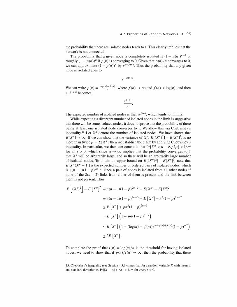
The expected number of isolated nodes is then ef (n), which tends to infinity. While expecting a divergent number of isolated nodes in the limit is suggestive
that there will be some isolated nodes, it does not prove that the probability of there being at least one isolated node converges to 1. We show this via Chebyshev’s inequality.15 Let Xn denote the number of isolated nodes. We have shown that E[Xn] → ∞. If we can show that the variance of Xn , E[(Xn)2] − E[Xn]2, is no more than twice μ = E[Xn], then we establish the claim by applying Chebyshev’s √ inequality. In particular, we then can conclude that Pr[Xn < μ − r 2μ] < 1/r2
for all r > 0, which since μ → ∞ implies that the probability converges to 1 that Xn will be arbitrarily large, and so there will be an arbitrarily large number of isolated nodes. To obtain an upper bound on E[(Xn)2] − E[Xn]2, note that E[Xn(Xn − 1)] is the expected number of ordered pairs of isolated nodes, which is n(n − 1)(1 − p)2n−3, since a pair of nodes is isolated from all other nodes if none of the 2(n − 2) links from either of them is present and the link between them is not present. Thus
E [ (Xn)2
] − E
[ Xn
]2 = n(n − 1)(1 − p)2n−3 + E[Xn] − E[Xn]2
= n(n − 1)(1 − p)2n−3 + E Xn − n 2(1 − p)2n−2
≤ E Xn + pn 2(1 − p)2n−3
= E Xn 1 + pn(1 − p)n−2
≤ E Xn 1 + (log(n) − f (n))e−log(n)+f (n)(1 − p)−2
≤ 2E Xn .
To complete the proof that t (n) = log(n)/n is the threshold for having isolated nodes, we need to show that if p(n)/t (n) → ∞, then the probability that there
15. Chebyshev’s inequality (see Section 4.5.3) states that for a random variable X with mean μ
and standard deviation σ , Pr[|X − μ| > rσ ] < 1/r2 for every r > 0.

∑ ∑
∑ ∑
∑ ∑
96 Chapter 4 Random-Graph Models of Networks
are isolated nodes tends to 0. It is enough to show this for p(n) = log(n)
n
+f (n) , where f (n) → ∞ but f (n)/n → 0.16 By a similar argument to the one above, we conclude that the expected number of isolated nodes is tending to e −f (n), which tends to 0. The probability of having Xn be at least one then has to tend to 0 as well for E[Xn] → 0.
To complete the proof of the theorem, we need to show that if p(n)/t (n) → ∞, then the chance of having any components of size 2 to size n/2 tends to 0. Let Xk
denote the number of components of size k, and write p(n) = log(n)+f (n) , where ∑n/2 n
f (n) → ∞ and f (n)/n → 0.17 It is enough to show that E[ k=2 Xk] → 0:
[ n/2 ]
n/2 ( )
E Xk ≤ n
(1 − p)k(n−k)
k k=2 k=2
n 3/4 ( ) n/2 ( )
= n
(1 − p)k(n−k) + n
(1 − p)k(n−k)
k k k=2 k=n3/4
n 3/4 ( )k n/2 ( )k
≤ ∑ en
e −knpek2 p + ∑ en
e −knp/2
k k k=2 k=n3/4
n 3/4 n/2 ( )k en≤ ek(1−f (n))k−ke 2k2log(n)/n + e −knp/2
k k=2 k=n3/4
≤ 3e −f (n) + n −n 3/4/5 ,
which tends to 0 in n.
The above proof used the specific structure of the Poisson random-network model fairly extensively. How far can we extend it to other random-network models? It is fairly clear that the argument used to prove Theorem 4.1 is not well suited to the configuration model. For the configuration model, under some reasonable bounds on degrees, each node acquires its specified degree with a probability approaching 1, which renders the above approach inapplicable. If the limiting degree distribution has a positive mass on nodes of degree 0 in the limit, then the network will not be connected, but otherwise it is not clear what will happen. For instance, if the associated P has mass on nodes of some bounded degree in the limit, then there is a nonvanishing probability that the network will not be connected. However, requiring that the mass on nodes of some bounded
16. Having no isolated nodes is clearly an increasing property, so that it holds for larger p(n). The reason for working with f (n)/n → 0 is to ensure that the approximation of (1 − p(n))n by e −np(n) is valid asymptotically. 17. Here again, we work with p(n) “near” the threshold, as this will establish that the resulting network is connected with a probability going to 1 for such p values, and then it holds for larger values of p.

∑
( )
∑
∏
∑
∑ ∑
97 4.2 Properties of Random Networks
degree vanish is not enough, as it is still possible that the network has a nontrivial probability of being disconnected.
The expected-degree model of Chung and Lu [156] is better suited for an analysis of connectivity. At least we can make some progress with regard to the threshold for the existence of isolated nodes, since the model is essentially a generalization of the Poisson random-network model that allows for different expected degrees across nodes (with the possibility of self-loops).
Recall that in the expected-degree model there are degree sequences of an expected degree for each node d1, . . . , dn. Let
n
Voln = di (4.4) i=1
denote the total expected degree of the network on n nodes. The probability of didja link between nodes i and j is then Voln , and so the probability that node i is
isolated is
∏ 1 −
didj .
Voln
j
By (4.4) the probability that a given node i is isolated is then approximately −di dj/Voln d2
j ie = e −di for large n (under the assumption that maxi Voln converges to 0, which is maintained under the expected-degree model). The probability that no node is isolated is then
(1 − e −di)
i
or approximately
− e −di e i .
This expression suggests a threshold such that if i e −di → 0, then there will be no isolated nodes, while if i e −di → ∞, then isolated nodes will occur.18 As a double-check of this hypothesis, let di = d(n) = log(n) + f (n) ∑for each i in the Poisson random-network setting (where p(n) = d(n)/n). Then i e −di = e −f (n), so if f (n) → ∞, there are no isolated nodes (and a connected network) and if f (n) → −∞, then the probability tends to 1 that there are isolated nodes. Indeed, this threshold corresponds to the one we found for the Poisson random-network model.
18. I am not aware of results on this question or the connectedness of the network under the expected-degree model. While it seems natural to conjecture that the threshold for the existence of isolated nodes is the same as the threshold for connectedness, the details need to be checked.

98 Chapter 4 Random-Graph Models of Networks
4.2.4 Giant Components
In cases for which the network is not connected, the components structure is of interest, as there will generally be many components. In fact, we have already shown that if the network is not connected in the Poisson random-network model, then there should be an arbitrarily large number of components. We also know from Section 4.2.2, that in this case there may still exist a giant component. Let us examine this in more detail and for a wider class of degree distributions.
In defining the size of a component, a convention is to call a component small if it has fewer than n 2/3/2 nodes, and large if it has at least n 2/3 nodes (e.g., see Chapter 6 in Bollobas [86]). The term giant component refers to the unique largest component, if there is one. This component may turn out to be small in some networks, but we are generally interested in giant components that involve nonvanishing fractions of nodes, which are necessarily “large” components.
The idea of there being a unique largest component is fairly easy to understand, in the case where these are large components. It relates to the proof of Theorem 4.1: for any two large sets of nodes (each containing at least n 2/3 nodes) it is very unlikely that there are no links between them, unless the overall probability of links is very small. For instance, in the Poisson random-network model the probability of having no links between two given large sets of nodes is no more than (1 − p)n 4/3
. If pn 4/3 → 0, then this expression is positive, but otherwise it tends to 0. Proving that the probability of not having two separate large components goes to 0 involves a bit more proof, but is relatively straightforward (see Exercise 4.7).
4.2.5 Size of the Giant Component in Poisson Random Networks
As already seen, it is not even clear whether each node is path-connected to every other node. Unless p is high enough relative to n, it is likely there exist pairs of nodes that are not path-connected. As a result, diameter is often measured with respect to the largest component of a network.19 But this also raises a question as to what the network looks like in terms of components. The answer is one of the deeper and more elegant results of the work of Erd¨ enyi. os and R´
To gain some impression of the size of the giant component, let us do a simple heuristic calculation.20 Form a Poisson random network on n − 1 nodes with a probability of any given link being p > 1/n. Now add a last node, and again connect this node to every other node with an independent probability p. Let q
be the fraction of nodes in the largest component of the n − 1 node network. As a fairly accurate approximation for large n, q will also be the fraction of nodes in the largest component of the n-node network. (The only possible exception is if the added node connects two large components that were not connected before. As argued above, the chance of having two components with large numbers of
19. This practice can result in some distortions; for instance, a network in which each node has exactly one link has a diameter much smaller than a network that has many more links. 20. The heuristic argument is based on Newman [503], but a very different and complete proof of the characterizing equation above the threshold for the emergence of the giant component can be found in Bollobas [86].

∑
99 4.2 Properties of Random Networks
nodes that are not connected to each other goes to 0 in n, given that p > 1/n.) The chance that this added node lies outside the giant component is the probability that none of its neighbors are in the giant component. If the new node has degree di
this probability converges to (1 − q)di , as n becomes large. As we can think of any node as having been added in this way, in a large network the expected frequency of nodes of degree di that end up outside the giant component is approximately (1 − q)di .21 So the overall fraction of nodes outside the giant component, 1 − q, can then be found by averaging (1 − q)di across nodes:22
1 − q = (1 − q)dP (d). (4.5) d
When we apply (4.5) to the Poisson degree distribution described by (1.4), the fraction of nodes outside the giant component is then approximated by the solution of
∑ e −(n−1)p((n − 1)p)d
1 − q = (1 − q)d. d!
d
Since
∑ ((n − 1)p(1 − q))d (n−1)p(1−q)= e ,
d! d
an approximation is described by the solution to
q = 1 − e −q(n−1)p. (4.6)
There is always a solution of q = 0 to (4.6). When the average degree is larger than 1 (i.e., p > 1/(n − 1)), and only then, there is also a solution for q that lies between 0 and 1.23 This case corresponds to a phase transition, in that the appearance of such a giant component comes above the threshold of (n − 1)p = 1. That is, there is a
21. There are steps omitted from this argument, as for any finite n the degrees of nodes in the network are correlated, as are their chances of being in the largest component conditional on their degree. For example, a node of degree 1 is in the giant component if and only if its neighbor is. If that neighbor has degree d, then it has d − 1 chances to be connected to a node in the giant component. Thus the calculation approaches (1 − q)d−1 for the neighbor to be in the giant component. To see a fuller proof of this derivation, see Bollobas [86]. 22. Here take the convention that 00 = 1, so that if q = 1, then the right-hand side of this equation is P(0). 23. To see this, let f (q) = 1 − e −q(n−1)p. We are looking for points q such that f (q) = q (known as fixed points). Since f (0) = 1 − e 0 = 0, q = 0 is always a fixed point. Next, note that f is increasing in q with derivative f ′(q) = (n − 1)pe−q(n−1)p and is strictly concave, as the second derivative is negative: f ′′(q) = −((n − 1)p)2 e −q(n−1)p. Since f (1) = 1 − e −(n−1)p < 1, f is a function that starts at 0 and ends with a value less than 1, and f is increasing and strictly concave. The only way in which it can ever cross the 45-degree line is if it has a slope greater than 1 when it starts, otherwise it will always lie below the 45-degree line, and 0 will be the only fixed point. The slope at 0 is f ′(0) = (n − 1)p, and so there is a q > 0 such that q = f (q) if and only if (n − 1)p is greater than 1.

100 Chapter 4 Random-Graph Models of Networks
marked difference in the structure of the resulting network depending on whether the average degree is greater than or less than 1. If the average degree is less than 1, then there is essentially no giant component: instead the network consists of many components that are all small relative to the number of nodes. If the average degree exceeds 1, then there is a giant component that contains a nontrivial fraction of all nodes (approximately described by (4.6)).
Note that if we let p(n − 1) grow (so that the average degree is unbounded as n
grows), then the solution for q tends to 1. Of course, that requires the average degree to become large. In a random network for which there is some bound on average degree, so that p(n − 1) is bounded, then q is between 0 and 1. For example, for a solution to q = 1 − e −q(n−1)p when n = 50 and p = .08, q roughly satisfies q = 1 − e −4q , or q is about .98. So an estimate for the size of the giant component is 49 nodes out of 50—which happens to match the realized network in Figure 1.6 exactly.
4.2.6 Giant Components in the Configuration Model
Understanding giant components more generally is especially important, as they play a central role in various problems of diffusion, and a giant component gives an idea of the most nodes that one might possibly reach starting from a single node. Let us examine giant components for more general random networks, using the configuration model as a basis.24 We work with randomly formed networks according to the configuration model on n nodes and will examine the limiting probability that the resulting networks have a giant component when n grows large. Consider a sequence of degree sequences, ordered by the number of nodes n, with corresponding degree distributions described by P n(d). Assume that these satisfy some conditions:
1. the degree distributions converge uniformly to a limiting degree distribution P that has a finite mean,
2. there exists ε such that P n(d) = 0 for all d > n 41 −ε ,
3. (d2 − 2d)P n(d) converges uniformly to (d2 − 2d)P (d), and
4. EP n[d2 − 2d] converges uniformly to its limit (which may be infinite).
An important aspect of such sequences is that the probability of having cycles in any small component tends to 0. Let us examine properties of the degree distribution that indicate when such networks exhibit a giant component. The following is a simple and informal derivation. A somewhat more complete derivation appears in Section 4.5.
The idea is to look for the threshold at which, starting at a random node, there is some chance of finding a nontrivial number of other nodes through tracing out expanding neighborhoods. Indeed, if a node is in a giant component, then exploring longer paths from the node should lead to the discovery of more and more nodes,
24. Similar results hold for the expected degree model of Chung and Lu [155], and under weaker restrictions on the set of admissible degree distributions, but they follow from a less intuitive argument.

⟨ ⟩
101 4.2 Properties of Random Networks
while if it is in a small component, then expanding neighborhoods will not result in finding many more nodes.
At or below the threshold at which the giant component just emerges, the components are essentially trees, and so each time we search along a link that has not been traced before, we will find a node that has not been previously visited. This fact allows us to analyze the component structure up to the point where the giant component emerges as if the network were a collection of trees. The following argument (due to Cohen et al. [161]) provides the idea behind there being negligible numbers of cycles below the threshold.25 Consider any link in the configuration model on n nodes. The probability that the link connects two nodes that were already connected in a component with s nodes (where s is the size of some component ignoring that link) is the probability that both of its end ( )2nodes lie in that component, which is proportional to s . Thus the fraction of ∑ ( si )2
n
links that end up on cycles is on the order of i n , where si is the size of ∑ siScomponent i in the network. This sum is less than 2 , where S is the size ∑ i n
of the largest component. Thus, since i si = n, we find that the proportion of links that lie on cycles is of an order no more than S/n. If we are at or below the threshold at which the giant component is just emerging, then with probability 1, S/n is vanishing for large n. Thus when we consider a sequence of degree distributions at or below the threshold of the emergence of the giant component, the components are essentially trees.26
To develop an estimate of component size as the network grows, let φ denote the limiting number of nodes that can be found on average by picking a link uniformly at random, picking with equal chance one of its end nodes, and then exploring all of the nodes that can be found by expanding neighborhoods from that end node. Given an absence of cycles, the number of new nodes reached by a link is the first node reached plus that node’s degree minus 1 (as one of its links points back to the original node) times φ, which indicates how many new nodes can be expected to be reached from each of the first node’s neighbors. Thus
∞ ∞φ = 1 +
∑ (d − 1)˜ = 1 +
∑ P(d)d (d − 1)φ. P (d)φ 〈d〉
d=1 d=1
We can rewrite this equation as
( d2 − 〈d〉)φ φ = 1 + ,〈d〉
or
1 φ = . (4.7)
2 − 〈d2〉 〈d〉
25. This is part of the informality of the derivation, and I refer the interested reader to Molloy and Reed [473] for a more complete proof. 26. The more rigorous result proven by Molloy and Reed [473] establishes that almost surely no component has more than one cycle.

⟨ ⟩ ⟨ ⟩
⟨ ⟩ ⟨ ⟩
⟨ ⟩
⟨ ⟩
∑
102 Chapter 4 Random-Graph Models of Networks
Now we deduce the threshold at which a giant component emerges. If φ has a finite solution, then for a node picked uniformly at random in the network, we expect to find a finite number of nodes that can be reached from one of its links. This places the node in a finite component. If φ does not have a finite solution, then we expect at least some nodes that are found uniformly at random to be in components that are growing without bound, which should occur at the threshold for the emergence of a giant component. For φ to have a finite solution it must be that 0 > d2 − 2 〈d〉. Thus if
d2 − 2 〈d〉 > 0, (4.8)
there is a giant component, and so the threshold is where d2 = 2 〈d〉. In the case of a Poisson distribution d2 = 〈d〉 + 〈d〉2, and so the giant compo
nent emerges when 〈d〉2 > 〈d〉, or 〈d〉 > 1. Indeed the threshold for the existence of a giant component for the Poisson random-network model is t (n) = 1/n, which corresponds to an average degree of 1.
In the case of a regular network, for which the degree sequences have full weight on some degree k, if we solve for d2 = 2 〈d〉 we find k2 = 2k, and so a threshold for a giant component is k = 2. Clearly, for k = 1we just have a set of dyads (paired nodes) and no giant component.
For a scale-free network, where the probability of degree d is of the form Pn(d) = cd−γ , we find that d2 diverges when γ < 3, and so generally there is a giant component regardless of the specifics of the distribution.
The arguments underlying the derivation of (4.5) were not specific to a Poisson distribution, and so for the configuration model when the probability of loops is negligible we still have as the approximation for the size of the giant component the largest q that solves
1 − q = (1 − q)dP (d). (4.9) d
Using this expression, there is much that we can deduce about how the size of the giant component changes with the degree distribution. For instance, if we change the distribution to place more weight on higher nodes (in the sense of first-order stochastic dominance; see Section 4.5.5), then the right-hand side expectation goes down for any value of q, and the new value of 1 − q that solves (4.9) has to decrease as well, which corresponds to a larger giant component, as detailed in Exercise 4.11. This trend makes sense, since we can think of such a modification as effectively adding links to the network, which should increase the size of the giant component. Interestingly, providing a mean-preserving spread in the degree distribution has the opposite effect, decreasing the size of the giant component. This result is a bit more subtle, but has to do with the fact that (1 − q)d
is a convex function of d. So spreading out the distribution leads to some higher-degree nodes that have a higher chance of being in a giant component, but also produces some lower-degree nodes with a much lower chance of being in the giant component. The key is that the convexity implies that there is more loss in probability from moving to lower-degree nodes than gain in probability from the high-degree nodes.

( ) ( )
� = ,
103 4.2 Properties of Random Networks
4.2.7 Diameter Estimation
Another important feature of a network is its diameter. This characteristic, as well as other related measures of distances between nodes, is important for understanding how quickly behavior or information can spread through a network, among other things.
Let us start by calculating the diameter of a network that makes such calculations relatively easy. Suppose that we examine a tree component so that there are no cycles. A method of obtaining an upper bound on diameter is to pick some node and then successively expand its neighborhood by following paths of length �, where � is increased until the paths are sufficiently long to reach all nodes. Then every node is at distance of at most � from our starting node and no two nodes can be at a distance of more than 2� from each other. Thus the diameter is bounded below by � and above by 2�.27 What this diameter works out to be will depend on the shape of the tree.
Let us explore a particularly nicely behaved class of trees. Consider a tree such that every node either has degree k or degree 1 (the “leaves”), and such that there is a “root” node that is equidistant from all of the leaves. Start from that root node.28 If we then move out by a path of 1, we have reached k nodes. Now, by traveling on all paths of length 2, we will have reached all nodes in the immediate neighborhoods of the nodes in the original node’s neighborhood: k + k(k − 1) or k2 nodes. Extending this reasoning, by traveling on all paths of length �, we will have reached
k + k(k − 1) + k(k − 1)2 + . . . + k(k − 1)�−1 .
This expression can be rewritten (see Section 4.5.1) as
(k − 1)� − 1 (
k ) ( )
k = (k − 1)� − 1 . k − 1 − 1 k − 2
We can thus find the neighborhood size needed to reach all nodes by finding the smallest � such that
k (k − 1)� − 1 ≥ n − 1.
k − 2
Approximating this equation provides a fairly accurate estimate of the neighborhood size needed to reach all nodes of (k − 1)� = n − 1, or
log(n − 1) log(k − 1)
and then the estimated diameter for this network is
log(n − 1)2 .
log(k − 1)
27. Note that we can easily see that both of these bounds can be reached. If the network is a line with an odd number of nodes, and we do this calculation from the middle node, then the diameter is exactly 2�, while if we start at one of the end nodes, then the diameter is exactly �. 28. Trees for which all nodes have either degree k or degree 1 are known as Cayley trees.

(
104 Chapter 4 Random-Graph Models of Networks
Newman, Strogatz, and Watts [510] follow similar reasoning to develop a rough estimate of the diameter of more general sorts of random networks by examining the expansion in the neighborhoods. The calculation presumes a tree structure, which in the Poisson random network setting we know not to be valid beyond the threshold at which the giant component emerges, and so it only gives an order of magnitude approximation near the threshold. Generally, obtaining bounds on diameters is a very challenging problem. We will encounter other situations where there are potential problems with the calculation as we proceed.
A randomly picked node i has an expected number of neighbors of 〈d〉 (recalling the 〈.〉 notation for the expectation operator). If we presume that nodes’ degrees are approximately independent, then each of these nodes has a degree described by the distribution P (d) from (4.2). Thus each of these nodes has an ex
pected number of neighbors (besides i) of ∑
(d − 1)˜ 〈d2〉−〈d〉 . So the d P (d), or 〈d〉 expected number of i’s second neighbors (who are at a distance of 2 from i) is
very roughly 〈d〉 〈d2〉−〈d〉 .29 Iterating, the expected number of kth neighbors is es〈d〉 timated by
〈d2〉 − 〈d〉 )k−1
〈d〉 ,〈d〉 so that expanding out to an �th neighborhood reaches
� ( )k−1∑ 〈d2〉 − 〈d〉〈d〉 (4.10)〈d〉 k=1
nodes. When this sum is equal to n − 1, it gives some idea of how far we need to go from a randomly picked node to hit all other nodes. This number gives us a crude estimate of the diameter of the largest component. Substituting for the sum of the series in (4.10) (see Section 4.5.1 for some facts about sums of series), we obtain an estimate of diameter as the � that solves ⎛( )�
⎞ 〈d2〉−〈d〉 − 1⎜ 〈d〉 ⎟〈d〉 ⎝ ( ) ⎠ = n − 1,〈d2〉−〈d〉 − 1〈d〉
or [ ( ) ] [ ] log (n − 1) 〈d2〉 − 2〈d〉 + 〈d〉2 − log 〈d〉2
� = [ ] . (4.11)log 〈d2〉 − 〈d〉 − log [〈d〉]
29. Thus there are several approximations. The tree structure is implicit in the assumption that each of these second neighbors are not already first neighbors. There is an assumption about the correlation in neighbors’ degrees implicit in the use of P to calculate these degrees. And the expected number of second neighbors is found by multiplying first neighbors times the expected number of their neighbors, again embodying some independence to have the expectation of a product equal the product of the expectations.

� = .
( )
4.3
4.3 An Application: Contagion and Diffusion 105
In cases for which 〈d2〉 is much larger than 〈d〉, (4.11) is approximately
� = log [n] + log [ 〈d2〉 ] − 2 log [〈d〉]
log [ 〈d2〉 ] − log [〈d〉] = log
[ n/〈d〉 ]
log [ 〈d2〉/〈d〉 ] + 1, (4.12)
although (4.12) should be treated with caution, as cycles are ignored, and when we are above the threshold for a giant component to exist (e.g., when 〈d2〉 is much larger than 2〈d〉), then there can be nontrivial clustering for some degree sequences.
If we examine (4.11) for the case of a Poisson random network, then 〈d2〉 − 〈d〉 = 〈d〉2, and then
〈d〉−1log (n − 1) 〈d〉 + 1
log(〈d〉) When 〈d〉 is substantially greater than 1, this is roughly log(n)/ log(〈d〉), which is very similar to the result for the regular tree example. If p is held constant, then as n increases, � decreases and converges to 1 from above. In that case we would estimate the diameter to be 2. In fact, it can be shown that for a constant p, this crude approximation is right on the mark: the diameter of a large random graph with constant p is 2 with a probability tending to 1 (see Corollary 10.11 in Bollobas [86]). Next let us consider the case in which the average degree is not exploding but instead is held constant so that p(n − 1) = 〈d〉 > 1. Then our estimate for diameter is on the order of log(n)/ log(〈d〉). Here the estimate is not as accurate.30 Applying this estimate to the network generated in Figure 1.6, where n = 50, p = .08, and the average degree is roughly 〈d〉 = 4, yields an estimated diameter of 2.8. While the calculation is only order of magnitude, this value is not far off for the largest component in Figure 1.6.
Developing accurate estimates for diameters, even for such completely random networks, turns out to be a formidable task that has been an active area of study in graph theory for the past four decades.31 Nevertheless, the above approximations reflect the fact that the diameter of a random network is likely to be “small” in the sense that it is significantly smaller than the number of nodes, and one can work with specific models to develop accurate estimates.
An Application: Contagion and Diffusion
To develop a feel for how some of the derivations from random networks might be useful, consider the following application. There is a society of n individuals. One of them is initially infected with a contagious virus (possibly even a computer virus). Let the network of interactions in the society be described by a Poisson random network with link probability p.
30. In this range of p, the network generally has a giant component but is most likely not completely connected. 31. See Chapter 10 in Bollobas [86] for a report on some of the results and references to the literature.

106 Chapter 4 Random-Graph Models of Networks
The initially infected person interacts with each of his or her neighbors. Some of the neighbors are immune to the virus, while others are not. Let any given individual be immune with a probability π . For instance, π might represent the fraction of indivduals with natural immunity, a percentage of people who have been vaccinated, or the percentage of people whose computers are not susceptible to the virus. This example is a variation on what is known as the Reed-Frost model in the epidemiology literature (see Bailey [28], as the work of Reed and Frost was never published), and is discussed in more detail in Section 7.2. The eventual spread of the disease can then be modeled by:
generating a Poisson random network on n nodes with link probability p,
deleting πn of the nodes (uniformly at random) and considering the remaining network, and
identifying the component that the initially infected individual lies in on this subnetwork.
This calculation is equivalent to examining a network on (1 − π)n nodes with a link probability of p and then examining the size of the component containing a randomly chosen node. Thus, given that the threshold for the emergence of a giant component is at p(1 − π)n = 1, then if p(1 − π)n < 1, we expect the disease to die out and only infect a negligible fraction of the population. In contrast, if p(1 − π)n > 1, then there is a nontrivial probability that it will spread to some fraction of the originally susceptible population. In particular, from (4.6) we know that for large n, if an agent in the giant component of the susceptible population is infected, then the expected size of the epidemic as a percentage of the nodes that are susceptible is approximated by the nonzero q that solves
q = 1 − e −q(1−π)np. (4.13)
log((1−π)n) Furthermore, from Theorem 4.1 if p > (1−π)n
, then with a probability approaching 1 (as n grows) the network of susceptible agents will be connected, and so all of the susceptible population will be infected.
While (4.13) is difficult to solve directly for q, we can rewrite the equation as
log(1 − q)(1 − π)np = . (4.14)
q
Then for different values of q on the right-hand side of (4.14), we find the corresponding levels of (1 − π)np that lead to those q values, which leads to Figure 4.8. The figure displays an initial threshold of (1 − π)np = 1. Nearly the entire population of susceptible individuals is connected as (1 − π)np approaches 5. So, for instance, if half the population is susceptible, and the average degree is greater than 10, then nearly all of the susceptible agents are interconnected, and the probability of them all becoming infected from a tiny initial seed is quite high.
It is also worth emphasizing that this model can also capture diffusion of various behaviors. For instance, define as susceptible someone who would buy a certain product if made aware of it. Then (1 − π) can be interpreted as the percentage of the population who would buy the product if everyone was aware of it. The size of the giant component from these calculations indicates the potential

107
4.4
4.4 Distribution of Component Sizes
0.0
0.2
1.00.0 2.0 3.0 4.0 5.00.5 1.5 2.5 3.5 4.5
0.4
0.6
0.8
1.0
Fraction of susceptible nodes in giant component
p(1–�)n
FIGURE 4.8 Fraction of the susceptible population in the largest component of a Poisson random network as a function of the proportion of susceptible nodes 1 − π times the link probability p times the population size n.
impact of informing a few agents in the population about the product, when they communicate by word of mouth with others and each individual is sure to learn about the product from any neighbor who buys it.
This analysis is built on contagion taking place with certainty between any infected and susceptible neighbors. When the transmission is probabilistic, which is the case in some applications, then the analysis needs to account for that. Such diffusion is discussed in greater detail in Chapter 7.
Distribution of Component Sizes*
The derivations in Section 4.2.6 provide an idea of when a giant component will emerge, and its size, but we might be interested in more information about the distribution of component sizes that emerge in a network. Again, we will see how important this is when we examine network-based diffusion in more detail in Chapter 7. Following Newman, Strogatz, and Watts [510], we can use probability generating functions to examine the component structure in more detail. (For readers not familiar with generating functions, it will be useful to read Section 4.5.9 before preceding with this section.)
This analysis presumes that adjacent nodes have independent degrees, and so it is best to fix ideas by referring to the configuration model, in which approximate independence holds for large n. Let the degree distribution be described by P .
Consider the following question. What is the size of the component of a node picked uniformly at random from the network? We answer this by starting at a

˜
∑ ˜( ) ∑ ˜
( )
108 Chapter 4 Random-Graph Models of Networks
node, picking one of its edges and examining the neighboring node, and then following the edges from that neighboring node and determining how many additional nodes we find. Then summing across the edges leaving the initial node, we have an idea of the expected size of the component. This method presumes a tree structure and is thus only a good approximation when the degree distribution is such that the number of cycles in the network is negligible.
Let Q denote the distribution of the number of nodes that can be found by picking an edge uniformly at random from the network, picking one of its nodes uniformly at random, and then counting that node plus all nodes that are found by following all paths from that node that do not use the original link. Let GQ(x)
denote the generating function associated with this distribution. Note that Q can be thought of in the following way. There is probability P (d)
that the node at the end of the randomly selected edge has degree d. In that case, it has d − 1 edges emanating from it. The number of additional nodes that can be found by starting from each such edge is a random variable Q.32 We now use some facts about generating functions to deduce the generating function of Q. In Section 4.5.9 (see (4.23)) it is shown that the generating function of the sum of d − 1 independent draws from the distribution of Q is the the generating function of Q raised to the power d − 1, so the generating function of additional nodes [ ]d−1found through the node if it happens to have degree d is GQ(x) . The overall distribution of the number of nodes found through the additional node is then given by a mixture of distributions: first pick some random d according to ˜[ ]d−1
P(d), and then draw a random variable from a distribution having generating function GQ(x)
(see (4.24)). So the generating function of the distribution of the additional nodes ∑ [ ]d−1found after the first one is d P (d) G(q) . Finally, we need to add one node for the first one found, and the generating function of a distribution of a random variable plus 1 is just x times the generating function of the random variable (see (4.25)). Thus the distribution function of the number of nodes found from one side of an edge picked uniformly at random is
GQ(x) = x P (d)[GQ(x)]d−1 .
d
Noting that GP GQ(x) = d P (d)[GQ(x)]d , we rewrite the above as33
GP GQ(x) GQ(x) = x
GQ(x)
or
( ( ))1/2 GQ(x) = xGP GQ(x) . (4.15)
32. There must be a large number of nodes for this approximation to be accurate, as otherwise there are fewer potential nodes to explore. 33. This equation appears to be different from (25) in Newman, Strogatz, and Watts [510], but
(.)Pin fact
G
G
Q(x) is the same as their G1 and allows for an easy derivation of (4.15).

∑ ( )
109 4.4 Distribution of Component Sizes
As Newman, Strogatz, and Watts [510] point out, finding a solution to (4.15) is in general impossible without knowing something more about the structure of P . However, we can solve for the expectation of Q, as that is simply G′ (1):
Q
GQ′ (x) = 2
1 ( xGP
( GQ(x)
))−1/2 ( GP
( GQ(x)
) + xG′ P
( GQ(x)
) G
Q′ (x)
) .
Thus recalling that G(1) = 1 for any generating function we find that ( ) G′
Q(1) = 1
2 1 + G′ P
(1) G′ Q(1) . (4.16)
Since G′ (1) = E [d] = 〈d2〉/〈d〉 it follows from (4.16) that when the expectation ˜ PP of Q does not diverge, it must be that
G′ Q(1) =
2 −1〈d2〉 . (4.17) 〈d〉
If 〈d2〉 ≥ 2〈d〉, then the expectation of Q diverges, and so (4.17) is no longer valid. Indeed this expression grows as 〈d2〉 approaches 2〈d〉. This behavior is consistent with (4.7).
Now we can calculate the average size of a component. Let H be the distribution of the size of the component of a node picked uniformly at random. Starting from a node picked uniformly at random, the degree is governed by P(d), the extended neighborhood size has generating function [GQ(x)]d , and we have to account for the initial node as well.34 Thus the generating function for H is
GH(x) = x P (d)[GQ(x)]d = xGP GQ(x) . (4.18) d
From (4.18) it follows that the average size of the component that a randomly selected node lies in is (if the average over Q does not diverge)
G′ (1) = 1 + G′ (1)G′ (1) = 1 + 〈d〉2 . (4.19)
H P Q 2〈d〉 − 〈d2〉 For Poisson random networks, 〈d〉 = (n − 1)p < 1 if the network is to remain
disconnected, and so this must also hold to prevent the average size of the component for diverging. Indeed, in the Poisson random-network model substituting 〈d〉 = (n − 1)p and 〈d2〉 = 〈d〉2 + 〈d〉, we find that average component size of a node picked uniformly at random is
1 G
H ′ (1) = 1 + .
1 − (n − 1)p
For instance, if (n − 1)p = 1/2 then the average component size is 3; if (n − 1)p = 9/10, then the average is 11.
34. The derivation of the distribution for Q was based on randomly picking a node at either end of an edge. Here, we are working out from a given node, but given (approximate) independence in degrees, the calculation is still valid.

∑
∑
∑
4.5
110 Chapter 4 Random-Graph Models of Networks
For scale-free networks, 〈d2〉 is generally large relative to 〈d〉 and diverges as n
grows. In that case, the expected component size diverges. The intuition behind this result is as follows. Even though the average degree might be low, if a given node has a neighbor, that neighbor is likely to have a high degree (as P(d)˜ = P(d)d/〈d〉, which in a scale-free network places great weight on the highest-degree nodes). It is then even more likely to have additional high-degree neighbors, and so forth.
Appendix: Useful Facts, Tools, and Theorems
This appendix contains a few mathematical definitions, formulas, theorems, and approximations that are useful in working with random networks.
4.5.1 Sums of Series
A geometric series is one in which a series of powers of x is summed, where x �= 1:
n∑ m − xn+1 i x
ax = a . 1 − x
i=m
Thus n
1 − xn+1 i ax = a .
1 − x i=0
For x < 1 it follows that ∞
i ax ax = ,
1 − x i=1
and ∞
i a ax = .
1 − x i=0
Another series of interest (especially for scale-free degree distributions) is
∞∑ 1 a . iγ
i=1 ∑∞ 1This is the Riemann zeta function, z(γ ) = 1 γ , which is convergent when γ is
greater than 1. A special case is γ = 1, when we can look at a truncated series
n∑ 1 = H , (4.20)ni
i=1
which is known as a harmonic number and has various approximations. For large n, an approximation of Hn is γ + log(n), where the γ of roughly .577 is the Euler-Mascheroni constant. The difference between this approximation and Hn tends

( )
( )
[∣∣∣∣∣ ∑ ∣∣∣∣∣
]
1 114.5 Appendix: Useful Facts, Tools, and Theorems
to 0. Equation (4.20) is useful in approximating some sequences such as
1 1 1 + + . . . + , (4.21) i + 1 i + 2 t
which can be written as Ht − Hi. For large t , (4.21) is approximately log(t) − log(i), or log(t/i).
4.5.2 The Exponential Function ex and Stirling’s Formula
The exponential function ex can be defined in various ways that provide useful formulas. Fixing x (at any positive, negative or complex value),
n x
lim 1 + = ex. n→∞ n
Another definition of ex is given by
∞∑ .
n! i=0
n x ex =
Stirling’s formula for large n is
√ n n
n! ∼ 2πn . e
4.5.3 Chebyshev’s Inequality and the Law of Large Numbers
Chebyshev’s inequality states that for a random variable X with mean μ and standard deviation σ ,
Pr[|X − μ| > rσ ] < 1/r2
for every r > 0. This inequality is easy to prove directly from the definition of standard deviation. Letting r =
σx , we can also write this as
Pr[|X − μ| > x] < σ 2/x2
for every x > 0. Chebyshev’s inequality leads to an easy proof of a version of the weak law of large numbers:
Theorem 4.2 (The weak law of large numbers) Let (X1, X2, . . .) be a sequence of independently distributed random variables such that E[Xi] = μ for all i and there is a finite bound B so that Var(Xi) ≤ B for all i. Then
Pr n i=1 Xi
n − μ > ε → 0n
for all ε > 0.

∑
∑
[∣∣∣∣∣ ∑
∣∣∣∣∣ ]
[ ∑ ]
( ) ( )
( )
√
√
112 Chapter 4 Random-Graph Models of Networks
XiProof of Theorem 4.2. Let S = n . Thenn i=1 n
Var(Xi) BVar(Sn ≤) = .
2n n i
Thus Var(Sn) → 0. By Chebyshev’s inequality, fixing any ε > 0,
nVar(Sn)XiPr − μ > ε ≤ → 0,
ε2n i=1
which establishes the claim.
A stronger conclusion is also possible. The weak law of large numbers just states that the probability that a sequence of observed sample means deviates from the true mean of the process tends to 0. This does not directly imply that there is a probability 1 that the sequence will converge. The strong law of large numbers provides this stronger conclusion. For a proof, see Billingsley [69].
Theorem 4.3 (The strong law of large numbers) Let (X1, X2, . . .) be a sequence of independently and identically distributed random variables such that E[Xi] = μ for all i. Then
n i=1 Xi
Pr lim = μ = 1. n
4.5.4 The Binomial Distribution
There are many situations in which we need to make use of the binomial distribution. This section defines the distribution and also provides an illustration of the law of large numbers.
Consider flipping a coin repeatedly, when the coin is not a “fair” coin, but instead has a probability of p of coming up heads and of 1 − p of coming up tails. A single flip is called a Bernoulli trial. In many instances we are interested in a set of flips. If we ask about the probability of a particular sequence of heads and tails being realized, say heads, tails, tails, heads, heads, . . ., where there are
m(1 − p)n−m. Noting that therem heads out of n flips, then its probability is p n!n n(read “n choose m,” where ) different orderings that haveare =
m!(n−m)!m m
m heads out of n flips of the coin, the probability that there are m heads if we flip it n times is
n mp (1 − p)n−m. m
The expected number of heads out of n flips is simply pn, while the standard deviation is np(1 − p).
Note also that the expected fraction of flips of the coin that come up heads is
simply p, and the standard deviation of this fraction out of n flips is p(1n −p) .

[ √ ]
[ √ ]
∑ ∑ ∑ ∑
∑ ∑
∫
4.5 Appendix: Useful Facts, Tools, and Theorems 113
Then applying Chebyshev’s inequality and letting X be the realized fraction of flips that come up heads,
Pr |X − p| > r p(1 − p)
< 1
.2n r
If r = n 1/4, then
p(1 − p) 1Pr |X − p| > < ,
1/4 1/2n n
and so with a large number of flips of the coin it is very unlikely that the realized fraction of heads will differ from p by very much, just as the law of large numbers states.
4.5.5 Stochastic Dominance and Mean-Preserving Spreads
Consider discrete distributions P and P with support on {0, 1, 2, . . .}.35 The concept of first-order stochastic dominance captures the idea that P is obtained by shifting mass from P to place it on higher values. The following conditions are equivalent:
f (d)P (d) ≥ f (d)P (d) for all nondecreasing functions f, x x 0 P(d) ≤ 0 P(d) for all x,∑∞ ∑∞ P(d) ≥ P(d) for all x,x x
and if they hold we say that P first order stochastically dominates P . The dominance is strict if the inequalities hold strictly for some x (or f ).
Note that if strict dominance holds, then f (d)P (d) > P (d) for anyf (d)strictly increasing f . An example of a degree distribution that (strictly) first-order stochastic dominates another is pictured in Figure 7.6.
The last two conditions are clearly equivalent and capture the idea that P places less weight on low values and thus more weight on higher values than does P . The idea that stochastic dominance provides higher expectations for all nondecreasing functions is not difficult to prove, as P shifts weight to higher values of the function f . The converse is easily seen using the third condition and a simple step function that has value 0 up to x and then 1 from x onward. Often referring to first-order stochastic dominance, the “first-order” is omitted and it is simply said that P
stochastically dominates P . The idea of second-order stochastic dominance is a less demanding relationship
than first-order stochastic dominance, and so it orders more pairs of distributions. It is implied by first-order stochastic dominance. Instead of requiring a higher expectation relative to all nondecreasing functions, it only requires a higher expectation relative to all nondecreasing functions that are also concave. This concept has deep
35. The extension of these definitions is straightforward to the case of more general probability .measures: simply substitute dP in the place of sums with respect to P .
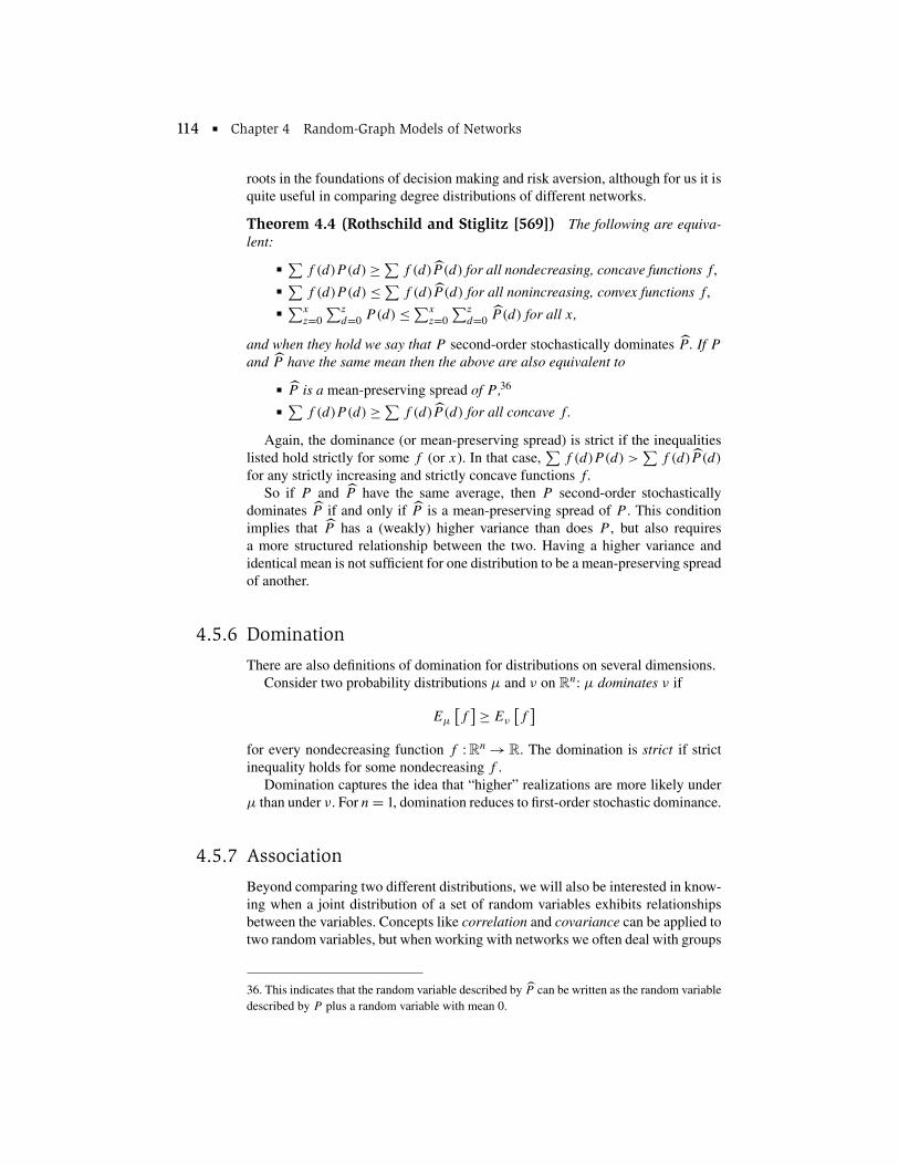
∑ ∑ ∑ ∑ ∑ ∑ ∑ ∑
∑ ∑
∑ ∑
[ ] [ ]
114 Chapter 4 Random-Graph Models of Networks
roots in the foundations of decision making and risk aversion, although for us it is quite useful in comparing degree distributions of different networks.
Theorem 4.4 (Rothschild and Stiglitz [569]) The following are equivalent:
f (d)P (d) ≥ f (d)P (d) for all nondecreasing, concave functions f,
f (d)P (d) ≤ f (d)P (d) for all nonincreasing, convex functions f, x z x z
d=0 P(d) ≤ P(d) for all x,z=0 z=0 d=0
and when they hold we say that P second-order stochastically dominates P . If P
and P have the same mean then the above are also equivalent to
P is a mean-preserving spread of P , 36
f (d)P (d) ≥ f (d)P (d) for all concave f.
Again, the dominance (or mean-preserving spread) is strict if the inequalities listed hold strictly for some f (or x). In that case, f (d)P (d) > P (d)f (d)for any strictly increasing and strictly concave functions f.
So if P and P have the same average, then P second-order stochastically dominates P if and only if P is a mean-preserving spread of P . This condition implies that P has a (weakly) higher variance than does P , but also requires a more structured relationship between the two. Having a higher variance and identical mean is not sufficient for one distribution to be a mean-preserving spread of another.
4.5.6 Domination
There are also definitions of domination for distributions on several dimensions. Consider two probability distributions μ and ν on Rn: μ dominates ν if
Eμ f ≥ Eν f
for every nondecreasing function f : Rn → R. The domination is strict if strict inequality holds for some nondecreasing f .
Domination captures the idea that “higher” realizations are more likely under μ than under ν. For n = 1, domination reduces to first-order stochastic dominance.
4.5.7 Association
Beyond comparing two different distributions, we will also be interested in knowing when a joint distribution of a set of random variables exhibits relationships between the variables. Concepts like correlation and covariance can be applied to two random variables, but when working with networks we often deal with groups
36. This indicates that the random variable described by P can be written as the random variable described by P plus a random variable with mean 0.

4.5 Appendix: Useful Facts, Tools, and Theorems 115
of variables. A notion that captures such relationships is association.The definition is due to Esary, Proschan, and Walkup [230].
Let μ be a joint probability distribution describing a random vector S = (S1, . . . Sn), where each Si is real-valued. Then μ is associated if
Covμ (f, g) = Eμ[f (S)g(S)] − Eμ[f (S)]Eμ[g(S)] ≥ 0
for all pairs of nondecreasing functions f : Rn → R and g : Rn → R. If S1, . . . , Sn are the random variables described by a measure μ that is as
sociated, then we say that S1, . . . , Sn are associated. Association of μ implies that S and Sj are nonnegatively correlated for any i and j , and it entails that alli
dimensions of S are nonnegatively interrelated.37
To establish strictly positive relationships, as opposed to nonnegative ones, Calvo-Armengol and Jackson [130] define a strong version of association. A partition of {1, . . . , n} captures which random variables are positively related (e.g., the components of nodes in a network). A probability distribution μ describing the random variables (S1, . . . Sn) is strongly associated relative to the partition if it is associated, and for any π ∈ and nondecreasing functions f and g
Covμ (f, g) > 0
when f is increasing in si for all s−i, g is increasing in sj for all s−j , and i and j are in π .
An implication of strong association is that S and Sj are positively correlatedi
for any i and j in π .
4.5.8 Markov Chains
There are many settings in which one considers a random process over time, the world can be described by a state, and the transition from one state to another depends only on the current state of the system and not how we got there. For the applications in this book, we are mainly concerned with finite-state systems. For instance, a network that describes a society at a given time can be thought of as a state. Alternatively, a state might describe some action of the agents in a network.
Let the finite set of states be denoted by S. If the state of the system is st = s at time t , then there is a well-defined probability that the system will be in state st+1 = s ′ at time t + 1 as a function only of the state st . Let be the n × n matrix describing these transition probabilities with entries
′ = Pr(s s ′ | s = s).ss t+1 = t
37. This concept is weaker than that of affiliation, which requires association when conditioning on various events. The weaker concept is useful in many network settings in which the states of nodes of a network are associated but are not affiliated. See Calvo-Armengol and Jackson [130] for an example and discussion.

∑
116 Chapter 4 Random-Graph Models of Networks
This matrix results in what is known as a (finite-state) Markov chain, where “Markov” refers to the property that the distribution of what will happen in the future of the system only depends on its current state, and not on how the current state came about. Markov chains have a number of applications and very nice properties, so they have been studied extensively. There are some basic facts about Markov chains that are quite useful.
The Markov chain is said to be irreducible when for any two states s ′ and s, if the system starts in state s ′ in some period, then there is a positive probability that it will reach s at some future date. Irreducibility corresponds to the strong connectedness of the associated directed graph in which the nodes are the states and s points to s ′ if s′s > 0.
An irreducible Markov chain is aperiodic if the greatest common divisor of its cycle lengths is 1, where the cycles are in the associated directed graph just described. Checking whether a system is aperiodic is equivalent to asking the following. Start in some state s at time 0 and list all the future dates for which there is a positive probability of being in this state again. If the answer for a state s is a list of dates with the greatest common divisor greater than 1, then that state is said to be periodic. If no state is periodic, then the Markov chain is aperiodic.38
Noting that the probability of starting in state s and ending in state s ′ in two periods is simply 2, we see by similar reasoning that the probability of starting in state s and ending in state s ′ in t periods is t . If t has all entries greater than 0 for some t , then it is clearly both irreducible and aperiodic, as it will then have all positive entries for all times thereafter. In contrast, if it never has all positive entries, then either it fails to be irreducible or it is periodic for some states.
An important theorem about Markov chains states that an irreducible and aperiodic finite-state Markov chain has what is known as a steady-state distribution (e.g., see Billingsley [69]). The steady state of the Markov process is described by a vector μ with dimension equal to the number of states, where μs is the probability of state s. The steady-state condition is that if the process is started at time 0 by randomly drawing the state according to the steady-state distribution, then the distribution over the state at time 1 will be given by the same distribution. That is,
μ ′ = μ ′,s s ss
s
or
μ = μ.
We can find the steady-state distribution as a left-hand unit eigenvector, noting that is a row-stochastic matrix (i.e., the elements of each row sum to 1).
Other useful facts about the steady-state distribution of a finite-state, irreducible, and aperiodic Markov chain include that it provides the long-run limiting average fraction of periods that the process will spend in each state regardless of
38. For those readers who want to master all of the definitions, verify that if a Markov chain has a finite number of states and is irreducible, then one state is periodic if and only if all states are periodic, and in that case they all have the same period (greatest common divisor of dates at which they have a probability of recurring).

∑
∑
∑
( )
4.5 Appendix: Useful Facts, Tools, and Theorems 117
the starting state; and regardless of where we start the system the probability of being in state s at time t as t increases goes to μs. Thus, when behavior can be described by a Markov chain, we have sharp predictions about behavior over the long run.
4.5.9 Generating Functions
Generating functions (also known as probability generating functions39) are useful tools for encapsulating the information about a discrete probability distribution and for calculating moments of the distribution and various other statistics associated with the distribution.
Let π(.) be a discrete probability distribution, which for our purposes has support in {0, 1, 2 . . .}. The generating function associated with π , denoted Gπ , is defined by
∞ [ ] Gπ(x) = π(k)xk = Eπ xk . (4.22)
k=0
Note that since π(.) is a probability distribution, Gπ(1) = 1. Moreover, Gπ has a number of useful properties. Taking various derivatives of it helps to recover the various expectations with respect to π :
∞G
π′ (x) = π(k)kxk−1 .
k=0
Thus
∞G
π′ (1) = π(k)k = Eπ [k] = 〈k〉.
k=1
More generally,40
( )m ∞d ∑
x Gπ = π(k)kmxk, dx
k=1
and so
[ ] dm ∣
E km = 〈km〉 = x Gπ ∣ x=1. dx
Next, suppose that we consider two independent draws of the random variable k and we want to know the sum of them. The probability that the sum is k is given
39. These are distinct from moment generating functions, which are defined by ∑∞
0 π(k)exk = [ ] k=e .Eπ xk ( )m
40. The notation x d Gπ indicates taking the derivative of Gπ with respect to x and thendx
multiplying the result by x, and then taking the derivative of the new expression and multiplying it by x, and so forth, for m iterations.
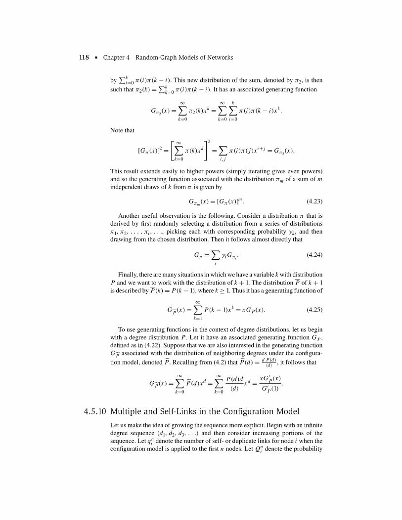
∑ ∑ ∑
∑ ∑
∑
∑
118 Chapter 4 Random-Graph Models of Networks
∑kby i=0 π(i)π(k − i). This new distribution of the sum, denoted by π2, is then ∑ksuch that π2(k) =
k=0 π(i)π(k − i). It has an associated generating function
∞ ∞ k
Gπ2(x) = π2(k)xk = π(i)π(k − i)xk.
k=0 k=0 i=0
Note that [ ]2∞[Gπ(x)]2 = π(k)xk = π(i)π(j)xi+j = Gπ2
(x).
k=0 i,j
This result extends easily to higher powers (simply iterating gives even powers) and so the generating function associated with the distribution πm of a sum of m
independent draws of k from π is given by
Gπ (x) = [Gπ(x)]m. (4.23)m
Another useful observation is the following. Consider a distribution π that is derived by first randomly selecting a distribution from a series of distributions π1, π2, . . . , πi, . . ., picking each with corresponding probability γk, and then drawing from the chosen distribution. Then it follows almost directly that
Gπ = γiGπi. (4.24)
i
Finally, there are many situations in which we have a variable k with distribution P and we want to work with the distribution of k + 1. The distribution P of k + 1 is described by P(k) = P(k − 1), where k ≥ 1. Thus it has a generating function of
∞G
P(x) = P(k − 1)xk = xGP(x). (4.25)
k=1
To use generating functions in the context of degree distributions, let us begin with a degree distribution P . Let it have an associated generating function GP , defined as in (4.22). Suppose that we are also interested in the generating function GP associated with the distribution of neighboring degrees under the configura
tion model, denoted P . Recalling from (4.2) that ˜ = d P (d)P (d) 〈d〉 , it follows that
∞ ∞∑ ˜ ∑ P(d)d d xG′
P(x)
GP (x) = P(d)xd = x = . 〈d〉 G′ (1)k=0 k=0 P
4.5.10 Multiple and Self-Links in the Configuration Model
Let us make the idea of growing the sequence more explicit. Begin with an infinite degree sequence (d1, d2, d3, . . .) and then consider increasing portions of the sequence. Let qi
n denote the number of self- or duplicate links for node i when the configuration model is applied to the first n nodes. Let Qn
i denote the probability

[ ] [∑ ∑ ]
[∑ ]
4.5 Appendix: Useful Facts, Tools, and Theorems 119
that under the configuration model, node i ≤ n has at least one self- or duplicate link, so that Qi
n = Pr[qin > 0]. We can then show the following.
Proposition 4.1 If a degree sequence (d1, d2, d3, . . .) is such that maxi≤n ndi/ n1/3 → 0, then maxi≤n Qi → 0.
This proposition is not true if we drop the restriction that maxi≤n di/n1/3 → 0 (see Exercise 4.2). The reason is that if some nodes have degrees that are too large relative to n, then nontrivial portions of the links involve these nodes, and the probability of self-links and/or multiple links can be nontrivial. Thus while the configuration model is useful when the degrees of nodes do not grow too large relative to the number of nodes, the degree sequences must be chosen carefully for the resulting multigraph to approximate a graph.
The proposition establishes that if maxi≤n di tends to 0, then the chance that any(n〈d〉)1/3
given node (including the largest ones) has a duplicate or self-link tends to 0. From this proposition, we can deduce that if self- and multiple links are deleted from the multigraph, then the proportion of nodes with the correct degree approaches 1 as the number of nodes grows, and the degree distribution converges to the desired distribution (pointwise, if there is an upper bound on degrees). However, convergence does not imply that the resultant multigraph will be a graph. When one aggregates across many nodes, there tend to be some duplicate and self-links, except under more extreme assumptions on the degree sequences; but there will not be many of them relative to the total number of links. To explore this idea in more detail, consider different statements about the probability of self- or multiple links under the configuration model:
1. Fixing a node and its degree, as the number of nodes grows the probability that the given node has any self- or multiple links vanishes. That is, Qn
i → 0.
2. The maximum probability across the nodes of having any self- or multiple links vanishes. That is, maxi≤n Qn
i → 0.
3. The fraction of nodes that have self- or duplicate links tends to 0. That is, for any ε > 0, Pr #{i ≤ n : qn > 0}/n > ε < ε for large enough n.i
4. The fraction of links that are self- or duplicate links tends to 0. That is, for
any ε > 0, Pr i≤n qin/ i≤n di > ε < ε for large enough n.
5. The probability of seeing any self- or multiple links vanishes. That is,
Pr i≤n qin > 0 → 0.
It is easy to see that (1) is true for any degree sequence, presuming that the sequence includes an infinite number of nodes with positive degree. Statement (2) is what is shown in Proposition 4.1, which then implies (3) based on the argument that when the probability across nodes of having self- or duplicate links goes to 0 uniformly across nodes, then it is impossible to expect a nontrivial fraction of nodes to have self- or multiple links (see Exercise 4.1). A similar argument establishes (4). The statement that would make our lives easiest in terms of ending up with a graph instead of a multigraph, (5), is only true under extreme conditions. To see why (5) generally fails, consider a degree sequence of (2, 2, 2, . . .), which is about as well behaved as one could want in terms of having a good chance of avoiding

[ ]
∑
120 Chapter 4 Random-Graph Models of Networks
self- and duplicate links. But even for this regular degree sequence there is still a nontrivial limiting probability of having at least one self-link. The probability that any given link is not a self-link is 1 − 2n
1 −1. To see this, start by connecting one
end of the link to some node, and then there are 2n − 1 equally likely entries in the full sequence of points to attach the other end of this link under the configuration model (see the sequence displayed at the beginning of Section 4.1.4). Only one of these choices leads to a self-link. Continue the process of randomly picking an entry to be one end of the link and picking a second entry for the other end. As we proceed, there will be at least n/2 links for which the initial node for the first end of the link does not yet have any link attached to it. For each of these links, an upper bound on the probability of not ending up with a self-link is 1 − 2n
1 −1. So
we have an upper bound on the probability of not ending up with any self-links in ( )n/2 the whole process, 1 − 2
1 n
, which converges to e −1/4.
The useful implication of statement (3) is that for a degree sequence that has a nice limiting degree distribution P(d),41 if we delete self- and duplicate links, then the proportion of nodes that have degree d converges almost surely to P(d)
(so Pr lim |pn(d) − P(d)| = 0 = 1, where pn(d) is the realized proportion of n
nodes with degree d after the deletion of duplicate and self-links).
Proof of Proposition 4.1. Let dn = maxi≤n di be the maximum degree up to
node n and 〈d〉n = i
n ≤n
di be the average degree through node n. We can find a
bound for the probability that any given node has a self- or a duplicate link. First, instead of thinking of the configuration process as picking two entries at random and matching them and then iterating, start by picking the first entry of the first element and randomly choosing a match for it, and then doing the same for the second remaining entry, and so forth. It is not hard to see that this process leads to the same distribution over matchings and thus of links. Consider the first node and its first link (isolated nodes can be discarded). The chance that the link is not a self- or duplicate link (so far) is 1 − (d1 − 1)/(n〈d〉n − 1), as only self-links need be considered. This probability is greater than 1 − dn/(n〈d〉n − dn). The chance that the second link (if it has degree greater than 1) is not a self- or duplicate link (so far), presuming the first one is not a self-link, is then
d1 − 2 di − 11 − − ,
n〈d〉n − 2 n〈d〉n − 2
where di is the degree of the node that the first link went to. This expression is greater than 1 − (2dn)/(n〈d〉n − dn). Continuing in this manner, we establishg a lower bound on the probability of self- or duplicate links:
41. There are various definitions of a limiting distribution that are useful. For instance, it could be that Pn(d) converges to P(d) for each d, but that it takes much longer to reach the limit for some ds compared to others. To make the above statement precise, consider a form of uniform convergence where maxd |P n(d) − P(d)| → 0. We can also work with other (weaker) definitions of convergence, such as pointwise convergence, weak convergence, or convergence in distribution (e.g., see Billingsley [68]).

( )
[ ]
121
4.6
4.6 Exercises
∏ ( dn
) j
1 − , n〈d〉n − dn
j=1,...,dn
which is larger than
(dn)2 dn
1 − . n〈d〉n − dn
If dn/((n〈d〉n − dn)1/3) tends to 0, then we can approximate the above expression by42
−( dn)dn)3/(n〈d〉n−e ,
dn
which tends to 1 if (and only if ) (n〈d〉n)1/3 tends to 0.
Exercises
4.1 Self- and Multiple Links in the Configuration Model ∗ Show that in the configuration model if maxi≤n Qi
n → 0, then the fraction of nodes that experience self-or multilinks vanishes as the population size n grows; or more specifically, for any ε > 0, Pr #{i ≤ n : qn > 0}/n > ε < ε for large enough n.i
4.2 A Degree Sequence That Always Has Large Nodes Consider the degree sequence (1, 1, 2, 4, 8, 16, . . .). Show that in the configuration model given node has a probability of self- or multiple links that tends to 0 as n becomes large, but for each n ≥ 2 there is some node with a significant probability of having a self-link or multiple links. That is, show that Qn
i → 0, but that Qnn → 1 for all n.
4.3 A Degree Sequence for the Power Distribution in the Configuration Model dn
Find a degree sequence that converges to a power distribution and for which (n〈d〉)1/3
tends to 0.
4.4 The Distribution of Neighbors’ Degrees in the Configuration and Expected-Degree Models Consider a constant degree sequence (d, d, d . . .). Form a random network by applying the configuration model and form another random network by applying the expected-degree model. Provide an expression for the resulting degree distributions in the limit as n grows (working with the resulting multigraph in the configuration model). Provide an expression for the limiting distribution P of the degree of a node found at either end of a uniformly randomly chosen link.
4.5 The Distribution of Neighbors’ Degrees
(a) Consider the Poisson random-network model on n nodes with a link probability of p. Consider a node i and a node j , which are fixed in advance.
42. We can approximate (1 − xr )x , when r → 0 and x does not decrease, by e −r . See Section
4.5.2 for approximating expressions.
122 Chapter 4 Random-Graph Models of Networks
Conditional on the link ij being present, what is the distribution of j ’s degree?
(b) Uniformly at random choose a node i out of those having at least one link, presuming that the network is nonempty. Randomly pick one of its neighbors (with equal probability on each neighbor). Argue that the conditional distribution of the node’s degree is different from the conditional distribution for j ’s degree that you found in part (a). What does this distribution converge to as n grows if p is set to keep the average degree constant (so that p = m/(n − 1) for some fixed m > 0)?
(c) Explain the difference between these two distributions.
4.6 A Threshold for Links in the Poisson Random-Network Model Show that t (n) = 1/n2 is a threshold function for there being at least one link in a Poisson random network.
4.7 There Is at Most One Giant Component in the Poisson Random-Network Model ∗ Consider the Poisson random-network model when p (as a function of n) is such that there exists m > 0 such that pn ≥ m for all n. Show that the probability of having more than one giant component vanishes as n grows.
4.8 Size of the Giant Component (a) Show that there is a solution to (4.9) of q = 1 if and only if P(0) = 0. (b) Find a nonzero solution to (4.9) when P(0) = 1/3 and P(2) = 2/3.
4.9 Estimating the Extent of an Infection in an Exponential Random-Network Model ∗ Consider a degree distribution given by
−d +1 e (1−π)m
P (d) = m
with support from (1 − π)m to ∞, which has a mean of 2(1 − π)m (which is derived in Section 5.1 as the distribution corresponding to a uniformly random network in which the number of nodes grows over time). Use (4.9) to estimate the percentage of susceptible nodes that will be infected when a random selection π of nodes are immune. Hint: See Section 4.5.1 for helpful formulas for sums of series.
4.10 Estimating the Diameter in an Exponential Random-Network Model Consider a degree distribution given by
−d +1 e m
P (d) = m
with support from m to ∞. Use (4.11) to estimate the diameter.
4.11 First-Order Stochastic Dominance and Increasing Giant Components
(a) Consider two degree distributions P and P , such that P first-order stochastically dominates P (see Section 4.5.5 if this definition is unfamiliar). Show

4.6 Exercises 123
that if q ′ and q are interior solutions to (4.9) relative to P and P , respectively, then q ≥ q ′ .43
(b) If P is a mean-preserving spread of P , and q ′ and q are interior solutions to (4.9) relative to P and P , respectively, how are q ′ and q ordered?
4.12 Mean-Preserving Spreads and Decreasing Diameters Consider two degree distributions P and P , such that P is a mean-preserving spread of P (see Section 4.5.5 if this definition is unfamiliar). Show that the solution to (4.11) under P is lower than that under P . Show that if we change “is a mean-preserving spread of” to “first-order stochastically dominates,” then the solutions to (4.11) cannot be ordered.
4.13 First-Order Stochastic Dominance and Decreasing Diameters ∗ Consider two finite-degree sequences in the expected-degree model of Section 4.1.5, with corresponding distributions P and P , such that P first-order stochastically dominates P . Show that the random networks associated with P have higher diameters in the sense of first-order stochastic dominance of the realized network diameters compared to those associated with P .
4.14 Component Sizes for a Family of Degree Distributions ∗
(a) Calculate 〈d2〉 using the degree distribution that has a distribution function of
F(d) = 1 − (rm)1+r (d + rm)−(1+r) ,
from (3.2), using this continuous distribution as an approximation for distributions with large n.
(b) Show that 〈d2〉 diverges when r < 1. Use the expression for 〈d2〉 and (4.19) to estimate the expected component size in large networks with such a degree distribution when r > 1 and for m = 〈d〉 such that 〈d2〉 < 2〈d〉.
43. To offer a complete proof to this statement, note that (4.9) can be written as a function 1 − q = H(1 − q), where you can show that H( ) is increasing and strictly convex and H(1) = 1..
Thus, you can show that it has at most one solution other than q = 0. Drawing a picture is helpful.


![Chapter 1 [in PDF format] - Princeton University Press](https://static.fdocuments.in/doc/165x107/6209148355c481469e65fe26/chapter-1-in-pdf-format-princeton-university-press.jpg)
![Introduction [in PDF format] - Princeton University Press](https://static.fdocuments.in/doc/165x107/6206198d8c2f7b173004968c/introduction-in-pdf-format-princeton-university-press.jpg)


