CHAPTER 4 MODELING AND ANALYSIS

LEARNING OBJECTIVES

.:. Understand the bask concepts of MSS modeling

.:. Describe how MSS models interact with data and the user .:.

Understand the different model classes

.:. Understand how to structure decision-making of a few alternatives

.:. Describe how spreadsheets can be used for MSS modeling and solution

.:. Explain what optimization, simulation, and heuristics are, and when and how to use them .:.

Describe how to structure a linear programming model

.:. Become familiar with some capabilities of linear programming and simulation packages .:.

Understand how search methods are used to solve MSS models

/

.:. Explain the differences between algorithms, blind search, and heuristics .:.

Describe how to handle multiple goals

.:. Explain what is meant by sensitivity, automatic, what-if analysis, and goal seeking .:.

Describe the key issues of model management

In this chapter, we describe the model base and its management, one of the major com-

ponents of DSS. We present this material with a note of caution: modeling can be a very

difficult topic and is as much an art as a science. The purpose of this chapter is not

necessarily for the reader to master the topics of modeling and analysis. Rather, the material

is geared toward gaining familiarity with the important concepts as they relate to business

intelligence/DSS. We walk through some basic concepts and definitions of modeling

before introducing the influence diagram, which can aid a decision-maker in sketching a

model of a situation and even solving it. We next introduce the idea of modeling directly in

spreadsheets. Only then do we describe the structure of some successful time-proven

models and methodologies: decision analysis, decision trees, optimization, search methods,

heuristic programming, and simulation. We next touch on some recent developments in

modeling tools and techniques and conclude with some important issues in model-base

management. We defer our discussion on the database and its management until the next

chapter. We have found that it is necessary to understand models and their use before

attempting to learn how to utilize data warehouses, OLAp, and data mining effectively.

144

CHAPTER 4 MODELING AND ANALYSIS 145

The chapter is organized as follows:

4.1 Opening Vignette: DuPont Simulates Rail Transportation System and

Avoids Costly Capital Expense

4.2 MSS Modeling

4.3 Static and Dynamic Models

4.4 Certainty, Uncertainty, and Risk 4.5

Influence Diagrams

4.6 MSS Modeling with Spreadsheets .

4.7 Decision Analysis of a Few Alternatives (Decision Tables and Decision Trees)

4.8 The Structure of MSS Mathematical Models 4.9

Mathematical Programming Optimization

4.10 Multiple Goals, Sensitivity Analysis, What-If, and Goal Seeking

4.11 Problem-Solving Search Methods

4.12 Heuristic Programming

4.13 Simulation

4.14 Visual Interactive Modeling and Visual Interactive Simulation 4.15

Quantitative Software Packages

4.16 Model Base Management

------------- 4.1 OPENING VIGNETTE: DUPONT SIMULATES RAIL TRANSPORTATION SYSTEM AND AVOIDS COSTLY CAPITAL EXPENSEl DuPont used simulation to avoid costly capital expenditures for rail car fleets as customer

demands changed. Demand changes could involve rail car purchases, better management

of the existing fleet, or possibly fleet size reduction. The old analysis method, past

experience, and conventional wisdom led managers to feel that the fleet size should be

increased. The real problem was that DuPont was not using its specialized rail cars

efficiently or effectively, not that there were not enough of them. There was immense

variability in production output and transit cycle time, maintenance scheduling, and order

sequencing. This made it difficult, if not impossible, to handle all the factors in a cohesive

and useful manner leading to a good decision.

The fleets of specialized rail cars are used to transport bulk chemicals from DuPont to

manufacturers. The cost of a rail car can vary from $80,000 for a standard tank car to more

than $250,000 for a specialized tanker. Because of the high capital expense, effective and

efficient use of the existing fleet is a must.

Instead of simply purchasing more rail cars, DuPont developed a ProModel simulation

model (ProModel Corporation, Orem, Utah, www.promodel.com) that represented the

firm's entire transportation system. It accurately modeled the variability inherent in

chemical production, tank car availability, transportation time, loading and unloading

time, and customer demand. A simulation model can provide a virtual environment in

which experimentation with various policies that affect the physical transportation system

can be performed before real changes are made. Changes can be made quickly and

inexpensively in a simulated world because relationships among the components of the

system are represented mathematically. It is not necessary to purchase expensive rail cars

to determine the effect.

I Adapted from Web site of ProModel Corporation, Orem, Utah,

www.promodel.corn, 2002.

http://www.promodel.corn,/

146 PART II DECISION SUPPORT SYSTEMS

ProModel allowed the company to construct simulation models easily and quickly (the

first one took just two weeks to develop) and to conduct what-if analyses. It also included

extensive graphics and animation capabilities. The simulation involved the entire rail

transportation system. Many scenarios were developed, and experiments were run. DuPont

experimented with a number of conditions and scheduling policies. Development of the

simulation model helped the decision-making team understand the entire problem (see

Banks et al.; 2001; Evans and Olson, 2002; Harrell et al., 2000; Law et al., 2000; Ross,

2003; Seila, Tadikamalla, and Ceric, 2003). The ProModel simulation accurately

represented the variability associated with production, availability of tank cars,

transportation times, and unloading at the customer site.

With the model, the entire national distribution system can be displayed graphically

(visual simulation) under a variety of conditions-especially the current ones and forecasted

customer demand. The simulation model helped decision-makers identify bottlenecks and

other problems in the real system. By experimenting with the simulation model, the real

issues were easily identified. The results convinced decisionmakers that a capital expense

was unjustified. In fact, the needed customer deliveries could still be made after

downsizing the fleet. Simulation drove this point home hard. After only two weeks of

analysis, DuPont saved $500,000 in capital investment that year.

Following the proven success of this simulation model, DuPont has started performing

logistics modeling on a variety of product lines, crossing division boundaries and political

domains. Simulation dramatically improved DuPont's logistics. The next step focused on

international logistics and logistics support for new market development. Savings in these

areas can be substantially higher.

.:. QUESTIONS FOR THE OPENING VIGNETTE

1. Why did the decision-makers initially feel that fleet expansion was the right deci-sion?

2. How do you think the decision-makers learned about the real system through model development? As a consequence, were they able tofocus better on the structure of the real system? Do you think their involvement in model building helped them in accepting the results? Why or why not?

3, Explain how simulation was used to evaluate the operation of the rail system before the changes were actually made.

4. How could the time compression capability of simulation help in this situation?

5. Simulation does not necessarily guarantee that an analyst will find the best solution. Comment on what this might mean to DuPont.

6. Once the system indicated that downsizing was a viable alternative, why do you think the managers bought into the system? Do you think that this is why the development team continues to work on other logistics problems? Explain.

- ~ 4.2 MSS MODELING The opening vignette illustrates a complex decision-making problem for which con-

ventional wisdom dictated an inferior decision alternative. By accurately modeling the rail

transportation system, decision-makers were able to experiment with different policies and

alternatives quickly and inexpensively. Simulation was the modeling approach used. The

DuPont simulation model was implemented with commercial soft-

CHAPTER 4 MODELING AND

ANALYSIS 147

ware, which is typical. The simulation approach saves DuPont a substantial amount of

money annually. Instead of investing in expensive rail cars and then experimenting with

how best to use them (also quite expensive), all the work was performed on a computer,

initially in two weeks. Before the first flight to the moon, the National Aeronautics and

Space Administration (NASA) performed countless simulations. NASA still simulates

space shuttle missions. General Motors now simulates all aspects of new car development

and testing (see Gallagher, 2002; Gareiss, 2002; Witzerman, 2001). And Pratt & Whitney

uses a simulated (virtual reality) environment in designing and testing engines for jet

fighters (Marchant, 2002). It is extremely easy to change a model of a physical system's

operation with computer simulation.

The DuPont simulation model was used to learn about the problem at hand, not

necessarily to derive new alternative solutions. The alternative solutions were known, but

were untested until the simulation model was developed and tested. Some other examples

of simulation are given by Van der Heijden et al. (2002) and Rossetti and Selandar (2001).

Van der Heijden et al. (2002) used an object-oriented simulation to design an automated

underground freight transportation system at Schiphol Airport (Amsterdam). Rossetti and

Selandar (2001) developed a simulation model that compared using human couriers to

robots in a university hospital. The simulation showed that the hospital could save over

$200,000 annually by using the robots. Simulation models can enhance an organization's

decision-making process and enable it to see the impact of its future choices. For example,

Fiat saves $1 million annually in manufacturing costs through simulation. The 2002 Winter

Olympics (Salt Lake City, Utah) used simulation to design security systems and bus

transportation for most of the venues. The predictive technology enabled the Salt Lake

Organizing Committee to model and test a variety of scenarios, including security

operations, weather, and transportationsystem design. Its their highly variable and complex

vehicle-distribution network. Savings were over $20 million per year. Benefits included

lower costs and improved customer service. (See promodel.com for details.)

Modeling is a key element in most DSS/business intelligence (also business analytics)

and a necessity in a model-based DSS. There are many classes of models, and there are

often many specialized techniques for solving each one. Simulation is a common modeling

approach, but there are several others. For example, consider the optimization approach

taken by Procter and Gamble (P&G) in redesigning its distribution system (Web Chapter).

P&G's DSS for its North America supply chain redesign includes several models:

A generating model (based on an algorithm) to make transportation cost esti-mates. This model is programmed directly in the DSS.

A demand forecasting model (statistically based).

A distribution center location model. This model uses aggregated data (a special modeling technique) and is solved with a standard linear/integer optimization package.

A transportation model (specialization of a linear programming model) to determine

the best shipping from product sources to distribution centers (fed to it from the

previous model) and hence to customers. It is solved using commercialsoftware and is

loosely integrated with the distribution location model. These two problems are

solved sequentially. The DSS must interface with commercial software and integrate

the models.

•• A financial and risk simulation model that takes into consideration some qualitative factors that require important human judgment.

A geographic information system (effectively a graphical model of the data) for a user

interface.


The Procter & Gamble situation demonstrates that a DSS can be composed of several

models, some standard and some custom built, used collectively to support strategic decisions

in the company. It further demonstrates that some models are built directly in the DSS software

development package, some need to be constructed externally to the DSS software, and others

can be accessed by the DSS when needed. Sometimes a massive effort is necessary to assemble

or estimate reasonable model data (about 500 P&G employees were involved over the course of

about a year), that the models must be integrated, that models may be decomposed and

simplified, that sometimes a suboptimization approach is appropriate, and finally, that human

judgment is an important aspect of using models in decision-making.

As is evident from theP&G situation and the IMERYS situation described in Case

Application 4.1, modeling is not a simple task [also see Stojkovic and Soumis (2001), who

developed a model for scheduling airline flights and pilots; Gabriel, Kydes and Whitman

(2001), who model the U.S. national energy-economic situation; and Teradata (2003), which

describes how Burlington Northern Santa Fe Corporation optimizes rail car performance

through mathematical (quantitative) models embedded in its OLAP tool]. The model builder

must balance the model's simplification and representation requirements so that it will capture

enough of reality to make it useful for the decisionmaker.

Applying models to real-world situations can save millions of dollars, or generate millions

of dollars in revenue. At American Airlines (AMR, Corp.), models were used extensively in

SABRE through the American Airlines Decision Technologies (AADT) Corp. AADT

pioneered many new techniques and their application, especially that of revenue management.

For example, optimizing the altitude ascent and descent profile for its planes saved several

million dollars per week in fuel costs. AADT saved hundreds of millions of dollars annually in

the early 1980s, and eventually its incremental revenues exceeded $1 billion annually,

exceeding the revenue of the airline itself (see Horner, 2000; Mukherjee, 2001; Smith et aI.,

2001; DSS in Action 4.1). Trick (2002) describes how Continental Airlines was able to recover

from the 9/11 disaster by using a system developed for snowstorm recovery. This system was

instrumental in saving millions of dollars.

United Airlines is in the process of creating a new generation of model-based DSS tools for planning, scheduling, and operations. United plans a major integration effort to determine the optimal schedule that can be designed and managed to maximize profitability. The key to integration and collaboration is a Web-based system called IPLAN that provides a platform for planners, schedulers, and other analysts across the airline to collaborate during the decision support process. It uses a suite of decision support tools:

1. SIMON optimally designs a flight network

and fleet assignment simultaneously.

2. ARM uses neighborhood search techniques for

optimal multi-objective fleet assignment.

3. AIRS 1M uses advanced statistical tools to

predict airline reliability.

4. SKYPATH performs optimal flight planning

for minimizing fuel burn on flights.

5. CHRONOS enables dynamic

multi-objective operations management.

Source: Adapted from Mukherjee (2001) .


Some major modeling issues include problem identification and environmental

analysis, variable identification, forecasting, the use of multiple models, model categories

(or appropriate selection), model management, and knowledge-based modeling.

IDENTIFICATION OF THE PROBLEM AND

ENVIRONMENTAL ANALYSIS

This issue was discussed in Chapter 2. One very important aspect is environmental

scanning and analysis, which is the monitoring, scanning, and interpretation of collected

information. No decision is made in a vacuum. It is important to analyze the scope of the

domain and the forces and dynamics of the environment. One should identify the

organizational culture and the corporate decision-making processes (who makes decisions,

degree of centralization, and so on). It is entirely possible that environmental factors have

created the current problem. Business intelligence (business analytics) tools can help

identify problems by scanning for them (see Hall, 2002a, 2000b; Whiting, 2003; the MSS

Running Case in DSS in Action 2.6; and DSS in Action 3.6, where we describe how

NetFlix.com creates usable environmental information for moviegoers). The problem must

be understood, and everyone involved should share the same frame of understanding

because the problem will ultimately be represented by the model in one form or another (as

was done in the opening vignette). Otherwir ~, the model will not help the decision-maker.

VARIABLE IDENTIFICATION

Identification of the model's variables (decision, result, uncontrollable, etc.) is critical, as

are their relationships. Influence diagrams, which are graphical models of mathematical

models, can facilitate this process. A more general form of an influence diagram, a

cognitive map, can help a decision-maker to develop a better understanding of the

problem, especially of variables and their interactions.

FORECASTING

Forecasting is essential for construction and manipulation of models because when a

decision is implemented, the results usually occur in the future. DSS are typically designed

to determine what will be, rather than as traditional MIS, which report what is or what was

(Chapter 3). There is no point in running a what-if analysis (sensitivity) on the past

because. decisions made then have no impact on the future. In Case Application 4.1, the

IMERYS clay processing model is "demand-driven." Clay demands are forecasted so that

decisions about clay production that affect the future can be made. Forecasting is getting

"easier" as software vendors automate many of the complications of developing such

models. For example, SAS has a High Performance Forecasting system that incorporates

its predictive analytics technology, ideally for retailers. This software is more automated

than most forecasting packages.

E-commerce has created an immense need for forecasting and an abundance of

available information for performing it. E-commerce activities occur quickly, yet infor-

mation about purchases is gathered and should be analyzed to produce forecasts. Part of the

analysis involves simply predicting demand; but product life-cycle needs and information

about the marketplace and consumers can be utilized by forecasting models to analyze the

entire situation, ideally leading to additional sales of products and services (see Gung,

Leung, Lin, and Tsai, 2002).

Hamey (2003) describes how firms attempt to predict who their best (i.e., most

profitable) customers are and focus in on identifying products and services that will

150

PART II DECISION SUPPORT SYSTEMS

appeal to them. Part of this effort involves identifying lifelong customer profitability.

These are important aspects of how customer relationship management and revenue-

management systems work.

Further details on forecasting can be found in a Web Chapter (prenhall.com/ turban).

Also see Faigle, Kern, and Still (2002).

MULTIPLE MODELS

A decision support system can include several models (sometimes dozens), each of which

represents a different part of the decision-making problem. For example, the Procter &

Gamble supply chain DSS includes a location model to locate distribution centers, a

product-strategy model, a demand forecasting model, a cost generation model, a financial

and risk simulation model, and even a GIS model. Some of the models are standard and

built into DSS development generators and tools. Others are standard but are not available

as built-in functions. Instead, they are available as freestanding software that can interface

with a DSS. Nonstandard models must be constructed from scratch. The P&G models were

integrated by the DSS, and the problem had multiple goals. Even though cost minimization

was the stated goal, there were other goals, as is shown by the way the managers took

political and other criteria into consideration when examining solutions before making a

final decision. Sodhi and Aichlmayr (2001) indicate how Web-based tools can be readily

applied to integrating and accessing supply chain models for true supply chain

optimization. Also see DSS in Action 4.1 for how United Airlines is integrating its models

into a major DSS tool.

MODEL CATEGORIES

Table 4.1 classifies DSS models into seven groups and lists several representative tech-

niques for each category. Each technique can be applied to either a static or a dynamic

model (Section 4.3), which can be constructed under assumed environments of certainty,

uncertainty, or risk (Section 4.4). To expedite model construction, one can use special

decision analysis systems that have modeling languages and capabilities embedded in

them. These include fourth-generation languages (formerly financial planning languages)

such as Cognos PowerHouse.

MODEL MANAGEMENT

Models, like data, must be managed to maintain their integrity and thus their applicability.

Such management is done with the aid of model base management systems (Section 4.16).

KNOWLEDGE-BASED MODELING

DSS uses mostly quantitative models, whereas expert systems use qualitative,

knowledge-based models in their applications. Some knowledge is necessary to construct

solvable (and therefore usable) models. We defer the description of knowledgebased

models until later chapters.

CURRENT TRENDS

There is a trend toward making MSS models completely transparent to the decisionmaker.

In multidimensional modeling and some other cases, data are generally shown in a

spreadsheet format (Sections 4.6 and 4.15), with which most decision-makers are familiar.

Many decision-makers accustomed to slicing and dicing data cubes are now


Category

Optimization of problems with few alternatives (Section 5.7)

Optimization via algorithm

(Section 5.8 and 5.9)

Optimization via an analytic

formula (Section 5.9)

Simulation (Sections 5.12

and 5.14)

Heuristics (Section 5.12)

Predictive models

(Web Chapter)

Other models

Process and Objective

Find the best solution from a small number of alternatives

Find the best solution from a large or an infinite number of alternatives using a step-by-step improvement process

Find the best solution in one step using a formula

Finding a good enough solution or the best among the alternatives checked using experimentation

Find a good enough solution using rules

Predict the future for a given scenario

Solve a what-if case using a formula

Representative Techniques

Decision tables, decision

trees

Linear and other mathematical programming models, network models

Some inventory models

Several types of simulation

Heuristic programming,

expert systems Forecasting

models, Markov analysis

Financial modeling, waiting lines

using online analytical processing (OLAP) systems that access data warehouses (see the

next chapter). Although these methods may make modeling palatable, they also eliminate

many important and applicable model classes from consideration, and they eliminate some

important and subtle solution interpretation aspects. Modeling involves much more than

just data analysis with trend lines and establishing relationships with statistical methods.

This subset of methods does not capture the richness of modeling, some of which we touch

on next, in several Web Chapters, and in Case Application 4.1.

- 4.3 STATIC AND DYNAMIC MODELS

DSS models can be classified as static or dynamic.

STATIC ANALYSIS

Static models take a single snapshot of a situation. During this snapshot everything occurs

in a single interval. For example, a decision on whether to make or buy a product is static in

nature (see the Web Chapter on Scott Housing's decision-making situation). A quarterly or

annual income statement is static, and so is the investment decision example in Section 4.7.

The IMERYS decision-making problem in Case Application 4.1 is also static. Though it

represents a year's operations, it occurs in a fixed time frame. The time frame can be

"rolled" forward, but it is nonetheless static. The same is true for the P&G decision-making

problem (Web Chapter). In the latter case, however, the impacts of the decisions may last

over several decades. Most static decision-making situations are presumed to repeat with

identical conditions (as in the BMI linear programming model described later). For

example,

152


process simulation begins with steady-state, which models a static representation of a

plant to find its optimal operating parameters. A static representation assumes that the

flow of materials into the plant will be continuous and unvarying. Steady-state

simulation is the main tool for process design, when engineers must determine the

best trade-off between capital costs, operational costs, process performance, product

quality, environmental and safety factors. (Boswell, 1999)

The stability of the relevant data is assumed in a static analysis.

DYNAMIC ANALYSIS

There are stories about model builders who spend months developing a complex,

ultra-large-scale, hard-to-solve static model representing a week's worth of a realworld

decision-making situation like sausage production. They deliver the system and present the

results to the company president, who responds, "Great! Well, that handles one week. Let's get

started on developing the 52-week model.t'-

Dynamic models represent scenarios that change over time. A simple example is a 5-year

profit-and-loss projection in which the input data, such as costs, prices, and quantities, change

from year to year.

Dynamic models are time-dependent. For example, in determining how many checkout

points should be open in a supermarket, one must take the time of day into consideration,

because different numbers of customers arrive during each hour. Demands must be forecasted

over time. The IMERYS model can be expanded to include multiple time periods by including

inventory at the holding tanks, warehouses, and mines. Dynamic simulation, in contrast to

steady-state simulation, represents what happens when conditions vary from the steady state

over time. There might be variations in the raw materials (e.g., clay) or an unforeseen (even

random) incident in some of the processes. This methodology is used in plant control design

(Boswell, 1999).

Dynamic models are important because they use, represent, or generate trends and patterns

over time. They also show averages per period, moving averages, and comparative analyses

(e.g., profit this quarter against profit in the same quarter of last year). Furthermore, once a static

model is constructed to describe a given situation--say, prod-, uct distribution can be expanded

to represent the dynamic nature of the problem (e.g., IMERYS). For example, the transportation

model (a type of network flow model) describes a static model of product distribution. It can be

expanded to a dynamic network flow model to accommodate inventory and backordering

(Aronson, 1989). Given a static model describing one month of a situation, expanding it to 12

months is conceptually easy. However, this expansion typically increases the model's

complexity dramatically and makes it harder, if not impossible, to solve. Also see Xiang and

Poh (2002).

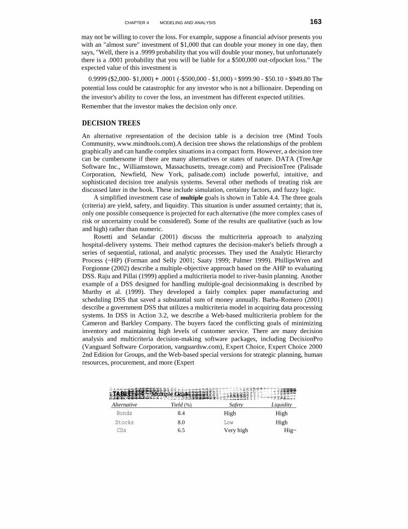
-~------------ 4.4 CERTAINTY, UNCERTAINTY, AND RISK3

Part of Simon's decision-making process described in Chapter 2 involves evaluating and

comparing alternatives, during which it is necessary to predict the future outcome of each

proposed alternative. Decision situations are often classified on the basis of

2Thanks to Dick Barr of Southern Methodist University, Dallas, Texas, for this one.

3Parts of Sections 4.4,4.5, and 4.7,4.9,4.12, and 4.13 were adapted from Turban and Meredith (1994).

37. CHAPTER4 MODELING AND ANALYSIS 153

what the decision-maker knows (or believes) about the forecasted results. Customary, we

classify this knowledge into three categories (Figure 4.1), ranging from complete

knowledge to total ignorance. These categories are

Certainty

Risk Uncertainty

When we develop models, any of these conditions can occur, and different kinds of

models are appropriate for each case. We discuss both the basic definitions of these terms

and some important modeling issues for each condition.

DECISION-MAKING UNDER CERTAINTY In decision-making under certainty, it is assumed that complete knowledge is available so

that the decision-maker knows exactly what the outcome of each course of action will be (as

in a deterministic environment). It may not be true that the outcomes are 100 percent

known, nor is it necessary to really evaluate all the outcomes, but often this assumption

simplifies the model and makes it tractable. The decision-maker is viewed as a perfect

predictor of the future because it is assumed that there is only one outcome for each

alternative. For example, the alternative of investing in U.S. Treasury bills is one for which

there is complete availability of information about the future return on the investment. Such

a situation occurs most often with structured problems with short time horizons (up to 1

year). Another example is that every time you park downtown, you get a parking ticket

because you exceed the time limit on the parking meteralthough once it did not happen.

This situation can still be treated as one of decisionmaking under certainty. Some problems

under certainty are not structured enough to be approached by analytical methods and

models; they require a DSS approach.

Certainty models are relatively easy to develop and solve, and can yield optimal

solutions. Many financial models are constructed under assumed certainty, even though the

market is anything but 100 percent certain. Problems that have an infinite (or a very large)

number of feasible solutions are extremely important and are discussed in Sections 4.9 and

4.12.

DECISION-MAKING UNDER UNCERTAINTY In decision-making under uncertainty, the decision-maker considers situations in which

several outcomes are possible for each course of action. In contrast to the risk situation, in

this case the decision-maker does not know, or cannot estimate, the proba-

Increasing knowledge

.•.

--------.- Decreasing knowledge

154


bility of occurrence of the possible outcomes. Decision-making under uncertainty is more difficult because of insufficient information. Modeling of such situations involves assessment of the decision-maker's (or the organization's) attitude toward risk (see Nielsen, 2003).

Managers attempt to avoid uncertainty as much as possible, even to the point of assuming it away. Instead of dealing with uncertainty, they attempt to obtain more information so that the problem can be treated under certainty (because it can be "almost" certain) or under calculated (assumed) risk. If more information is not available, the problem must be treated under a condition of uncertainty, which is less definitive than the other categories.

DECISION-MAKING UNDER RISK (RISK ANALYSIS)

A decision made under risk" (also known as a probabilistic or stochastic decisionmaking situation) is one in which the decision-maker must consider several possible outcomes for each alternative, each with a given probability of occurrence. The longrun probabilities that the given outcomes will occur are assumed to be known or can be estimated. Under these assumptions, the decision-maker can assess the degree of risk associated with each alternative (called calculated risk). Most major business decisions are made under assumed risk. Risk analysis can be performed by calculating the expected value of each alternative and selecting the one with the best expected value. Several techniques can be used to deal with risk analysis (see Drummond, 2001; Koller, 2000; Laporte, Louveeaux, and Van Hamme, 2002). They are discussed in Sections 4.7 and 4.13.

--~-----~---- 4.5 INFLUENCE DIAGRAMS

Once a decision-making problem is understood and defined, it must be analyzed. This can best be done by constructing a model. Just as a flowchart is a graphical representation of computer program flow, an influence diagram is a map of a model (effectively a model of a model). An influence diagram is a graphical representation of a model used to assist in model design, development, and understanding. An influence diagram provides visual communication to the model builder or development team. It also serves as a framework for expressing the exact nature of the relationships of the MSS model, thus assisting a modeler in focusing on the model's major aspects, and can help eliminate the less important from consideration. The term influence refers to the dependency of a variable on the level of another variable. Influence diagrams appear in several formats. The following description has evolved into a standard format (see the Decision Analysis Society Web site, faculty.fuqua.duke.edu/daweb/dasw6..htm; the Hugin Expert A/S (Aalborg, Denmark) Web site, developer.hugin.com/tutorialsl ID_example/; and the Lumina Decision Systems (Los Gatos, California) Web site, www.lumina.com/software/ infl uencediagrams.h tml):

40ur definitions of the terms risk and uncertainty were formulated by F. H. Knight of the University of Chicago in 1933. There are other, comparable definitions in use.

http://www.lumina.com/software/


Rectangle = decision variable

o Circle = uncontrollable or intermediate variable o Oval = result [outcome] variable: intermediate or final

The variables are connected with arrows that indicate the direction of influence (rela-

tionship). The shape of the arrow also indicates the type of relationship. The following are

typical relationships:

o Certainty

• lJncertainty

• Random (risk) variable: place a tilde (-) above the variable's name.

Preference (usually between outcome variables): a double-line arrow ~. Arrows can be one-way or two-way (bidirectional), depending on the direction of

influence of a pair of variables.

Influence diagrams can be constructed with any degree of detail and sophistication.

This enables the model builder to map all the variables and show all the relationships in the

model, as well as the direction of the influence. They can even take into consideration the

dynamic nature of problems (see Glaser and Kobayashi, 2002; Xiang and Poh, 2002).

38.

156 PART II DECISION SUPPORT SYSTEMS < -,

r--;» Amount used in advertisement

Unit price

An influence diagram for this simple model is shown in Figure 4.2.

SOFTWARE There are several software products that create and maintain influence diagrams. The solution process of these products transforms the original problem into graphical form. Representative products are

Analytica (Lumina Decision Systems, Los Altos, California, lumina. com). Analytica supports hierarchical diagrams, multidimensional arrays, integrated documentation, and parameter analysis.

DecisionPro (Vanguard Software Corporation, Cary, North Carolina,

vanguardsw.com). DecisionPro builds near-influence diagrams. The user decomposes

a problem into a hierarchical tree structure (thus defining the relationships among

variables). At the bottom, the variables are assigned values, or their values can be

randomly generated. DecisionPro is an integrated tool that includes a wide range of

decision-making techniques: linear programming, simulation, forecasting, and

statistical analysis. DATA and Data Pro (TreeAge Software Inc., Williamstown, Massachusetts,

treeage.com). DATA includes influence diagrams, decision trees, simulation models,

and others. It integrates with spreadsheets and Web pages.

iDecide (Definitive Software Inc., Broomfield, Colorado, definitivesoftware.com). Definitive Software's iDecide creates influence diagram-based decision models with bidirectional integration with Excel spreadsheets. The models can go directly from influence diagrams to Monte Carlo methods.


Precision Tree (Palisade Corporation, Newfield, New York, palisade.com).

PrecisionTree creates influence diagrams and decision trees directly in an Excel

spreadsheet. '

See faculty.fuqua.duke.edu/daweb/dasw6.htm for more. Downloadable demos are

available from each vendor's Web site. All of these Web-enabled systems create models

with a treelike structure in such a way that the model can be easily developed and

understood. Influence diagrams help focus on the important variables and their

interactions. In addition, these software systems can generate a usable model and solve it

without converting it for solution by a specialized tool. For example, Analytica lets the

model builder describe blocks of the model and how they influence the important result

variables. These submodel blocks are disaggregated by a model builder constructing a

more detailed model. Finally, at the lowest level, variables are assigned values (see the

Lumina Decision Systems Web site, lumina.com). In Figure 4.3a, we show an example of a

marketing model in Analytica. This model includes a price submodel and a sales submodel,

which appear in Figures 4.2b and 4.2c, respectively.

See the "2002 Decision Analysis Survey" in ORiMS Today, June 2002 (updated

annually and available online at lionhrtpub.com/orms/) for a survey of decision-analysis

software that includes influence diagrams. Also see Maxwell (2002). We next turn to an

important implementation vehicle for models: the spreadsheet.

Courtesy of Lumina Decision Systems, Los Altos, CA.

158 PART" DECISION SUPPORT SYSTEMS



-_._._._._---------- 4 .. 6 MSS MODELING WITH SPREADSHEETS

Models can be developed and implemented in a variety of programming languages and systems. These range from third-, fourth-, and fifth-generation programming languages to CASE systems and other systems that automatically generate usable software. We focus primarily on spreadsheets (with their add-ins), modeling languages, and transparent data analysis tools.


With their strength and flexibility, spreadsheet packages were quickly recognized as

easy-to-use implementation software for the development of a wide range of applications

in business, engineering, mathematics, and science. As spreadsheet packages evolved,

add-ins were developed for structuring and solving specific model classes. These add-ins

include Solver (Frontline Systems Inc., Incline Village, Nevada) and What'sBest! (a

version of Lindo, Lindo Systems Inc., Chicago, Illinois) for performing linear and

nonlinear optimization, Braincel (Promised Land Technologies, Inc., New Haven,

Connecticut) for artificial neural networks, Evolver (Palisade Corporation, Newfield, New

York) for genetic algorithms, and @Risk (Palisade Corporation, Newfield, New York) for

performing simulation studies. Because of fierce market competition, the better add-ins are

eventually incorporated directly into the spreadsheets (e.g., Solver in Excel is the

well-known GRG"2 nonlinear optimization code).

The spreadsheet is the most popular end-user modeling tool (Figure 4.4) because it

incorporates many powerful financial, statistical, mathematical, and other functions.

Spreadsheets can perform model solution tasks like linear programming and regression

analysis. The spreadsheet has evolved into an important tool for analysis, planning, and

modeling. (See Denardo, 2001; Hsiang, 2002; Monahan, 2000; Winston and Albright,

2000.)

Other important spreadsheet features include what-if analysis, goal seeking, data

management, and programmability (macros). It is easy to change a cell's value and

immediately see the result. Goal seeking is performed by indicating a target cell, its desired

value, and a changing cell. Rudimentary database management can be performed, or parts

of a database can be imported for analysis (which is essentially how OLAP works with

multidimensional data cubes; in fact, most OLAP systems have the

160


look-and-feel of advanced spreadsheet software once the data are loaded). The pro-gramming productivity of building DSS can be enhanced with the use of templates, macros, and other tools.

Most spreadsheet packages provide fairly seamless integration by reading and writing

common file structures that allow easy interfacing with databases and other tools.

Microsoft Excel and Lotus 1-2-3 are the two most popular spreadsheet packages.

In Figure 4.4 we show a simple loan calculation model (the boxes on the spreadsheet

describe the contents of the cells containing formulas). A change in the interest rate

(performed by typing in a new number in cell E7) is immediately reflected in the monthly

payment (in cell E13). The results can be observed and analyzed immediately. If we

require-a specific monthly payment, goal seeking (Section 4.10) can be used to determine

an appropriate interest rate or loan amount.

Static or dynamic models can be built in a spreadsheet. For example, the monthly loan

calculation spreadsheet shown in Figure 4.4 is static. Although the problem affects the

borrower over time, the model indicates a single month's performance, which is replicated.

A dynamic model, on the other hand, represents behavior over time. The loan calculations

in the spreadsheet shown in Figure 4.5 indicate the effect of prepayment on the principal

over time. Risk analysis can be incorporated into spreadsheets by using built-in random

number generators to develop simulation models (see Section 4.13, and the Web Chapters

describing an economic order-quantity simulation model under assumed risk and a

spreadsheet simulation model of cash flows).

LeBlanc, Randalls, and Swann (2000) describe an excellent example of a modelbased

DSS developed in a spreadsheet. It assigns managers to projects for a major construction

firm. By using the system, the company did not have to replace a manager


ANALYSIS

161

who resigned and thus substantially reduced travel costs. Buehlmann, Ragsdale, and Gfeller (2000) describe a spreadsheet-based DSS for wood panel manufacturing. This system handles many complex real-time decisions in a dynamic shop floor environment. Portucel Industrial developed a complete spreadsheet-based DSS for planning and scheduling paper production. See DSS in Action 3.8 and Respicio, Captivo, and Rodrigues (2002).

Spreadsheets were developed for personal computers, but they also run on larger

computers. The spreadsheet framework is the basis for multidimensional spreadsheets and

OLAP tools, which are described in the next chapter.

--~~---------~----- 4.7 DECISION ANALYSIS OF A FEW ALTERNATIVES (DECISION TABLES AND DECISION TREES)

Decision situations that involve a finite and usually not too large number of alternatives are modeled by an approach called decision analysis (see Arsham, 2003a, 2003b; and the Decision Analysis Society Web site, faculty.fuqua.duke.edu/daweb/). Using this approach, the alternatives are listed in a table or a graph with their forecasted contributions to the goal(s) and the probability of obtaining the contribution. These can be evaluated to select the best alternative.

Single-goal situations can be modeled with decision tables or decision trees.

Multiple goals (criteria) can be modeled with several other techniques described later.

DECISION TABLES

Decision tables area convenient way to organize information in a systematic manner. For example, an investment company is considering investing in one of three alternatives: bonds, stocks, or certificates of deposit (CDs). The company is interested in one goal: maximizing the yield On the investment after one year. If it were interested in other goals, such as safety or liquidity, the problem would be classified as one of multicriteria decision

analysis (Koksalan and Zionts, 2001) (see DSS in Action 3.2 and 4.1; Dias and Climaco, 2002).

The yield depends on the state of the economy sometime in the future (often called the

state of nature), which can be in solid growth, stagnation, or inflation. Experts estimated the

following annual yields:

If there is solid growth in the economy, bonds will yield 12 percent, stocks 15 per-cent, and time deposits 6.5 percent.

If stagnation prevails, bonds will yield 6 percent, stocks 3 percent, and time deposits 6.5 percent.

If inflation prevails, bonds will yield 3 percent, stocks will bring a loss of 2 per-cent, and time deposits will yield 6.5. percent.

The problem is to select the one best investment alternative. These are assumed to be discrete alternatives. Combinations such as investing 50 percent in bonds and 50 percent in stocks must be treated as new alternatives.

The investment decision-making problem can be viewed as a two-person game (see

Kelly, 2002). The investor makes a choice (a move) and then a state of nature occurs

(makes a move). The payoff is shown in a table representation (Table 4.2) of a


Alternative

State of Nature (Uncontrollable Variables)

Solid Growth (%) Stagnation (%) Inflation (%)

Bonds

Stocks

CDs

12.

0

15.

0

6.5

6.

0

3.

0

6.5

3.0

-2.0

6.5

mathematical model. The table includes decision variables (the alternatives), uncontrollable

variables (the states of the economy, e.g., the environment), and result variables (the

projected yield, e.g., outcomes). All the models in this section are structured in a

spreadsheet framework.

If this were a decision-making problem under certainty, we would know what the

economy will be and could easily choose the best investment. But this is not the case, and

so we must consider the two situations of uncertainty and risk. For uncertainty, we do not

know the probabilities of each state of nature. For risk, we assume that we know the

probabilities with which each state of nature will occur.

TREATING UNCERTAINTY

There are several methods of handling uncertainty. For example, the optimistic approach

assumes that the best possible outcome of each alternative will occur and then selects the

best of the bests (stocks). The pessimistic approach assumes that the worst possible

outcome for each alternative will occur and selects the best of these (CDs). Another

approach simply assumes that all states of nature are equally likely. See Clemen and Reilly

(2000), Goodwin and Wright (2000), Kontoghiorghes, Rustem, and Siokos (2002). There are

serious problems with every approach for handling uncertainty. Whenever possible, the

analyst should attempt to gather enough information so that the problem can be treated

under assumed certainty or risk.

TREATING RISK

The most common method for solving this risk analysis problem is to select the alternative

with the greatest expected value. Assume that experts estimate the chance of solid growth

at 50 percent, that of stagnation at 30 percent, and that of inflation at 20 percent. Then the

decision table is rewritten with the known probabilities (Table 4.3). An expected value is

computed by multiplying the results (outcomes) by their respective probabilities and

adding them. For example, investing in bonds yields an expected return of 12(0.5) + 6(0.3)

+ 3(0.2) = 8.4 percent.

This approach can sometimes be a dangerous strategy, because the "utility" of each

potential outcome may be different from the "value." Even if there is an infinitesimal

chance of a catastrophic loss, the expected value may seem reasonable, but the investor

Alternative Solid Growth, .50(%) Stagnation, .30(%) Inflation, .20(%) Expected Value (%)

Bonds 12.0 6.0 3.0 8.4 (maximum)

Stocks 15.0 3.0 -2.0 8.0

CDs 6.5 6.5 6.5 6.5


may not be willing to cover the loss. For example, suppose a financial advisor presents you

with an "almost sure" investment of $1,000 that can double your money in one day, then

says, "Well, there is a .9999 probability that you will double your money, but unfortunately

there is a .0001 probability that you will be liable for a $500,000 out-ofpocket loss." The

expected value of this investment is

0.9999 ($2,000- $1,000) + .0001 (-$500,000 - $1,000) = $999.90 - $50.10 = $949.80 The

potential loss could be catastrophic for any investor who is not a billionaire. Depending on

the investor's ability to cover the loss, an investment has different expected utilities.

Remember that the investor makes the decision only once.

DECISION TREES

An alternative representation of the decision table is a decision tree (Mind Tools

Community, www.mindtools.com).A decision tree shows the relationships of the problem

graphically and can handle complex situations in a compact form. However, a decision tree

can be cumbersome if there are many alternatives or states of nature. DATA (TreeAge

Software Inc., Williamstown, Massachusetts, treeage.com) and PrecisionTree (Palisade

Corporation, Newfield, New York, palisade.com) include powerful, intuitive, and

sophisticated decision tree analysis systems. Several other methods of treating risk are

discussed later in the book. These include simulation, certainty factors, and fuzzy logic.

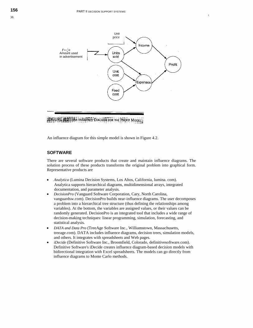
A simplified investment case of multiple goals is shown in Table 4.4. The three goals

(criteria) are yield, safety, and liquidity. This situation is under assumed certainty; that is,

only one possible consequence is projected for each alternative (the more complex cases of

risk or uncertainty could be considered). Some of the results are qualitative (such as low

and high) rather than numeric.

Rosetti and Selandar (2001) discuss the multicriteria approach to analyzing

hospital-delivery systems. Their method captures the decision-maker's beliefs through a

series of sequential, rational, and analytic processes. They used the Analytic Hierarchy

Process (~HP) (Forman and Selly 2001; Saaty 1999; Palmer 1999). PhillipsWren and

Forgionne (2002) describe a multiple-objective approach based on the AHP to evaluating

DSS. Raju and Pillai (1999) applied a multicriteria model to river-basin planning. Another

example of a DSS designed for handling multiple-goal decisionmaking is described by

Murthy et al. (1999). They developed a fairly complex paper manufacturing and

scheduling DSS that saved a substantial sum of money annually. Barba-Romero (2001)

describe a government DSS that utilizes a multicriteria model in acquiring data processing

systems. In DSS in Action 3.2, we describe a Web-based multicriteria problem for the

Cameron and Barkley Company. The buyers faced the conflicting goals of minimizing

inventory and maintaining high levels of customer service. There are many decision

analysis and multicriteria decision-making software packages, including DecisionPro

(Vanguard Software Corporation, vanguardsw.com), Expert Choice, Expert Choice 2000

2nd Edition for Groups, and the Web-based special versions for strategic planning, human

resources, procurement, and more (Expert

Alternative Yield (%) Safety Liquidity

Bonds 8.4 High High

Stocks 8.0 Low High

CDs 6.5 Very high Hig~

39. 164 PART II DECISION SUPPORT SYSTEMS

Choice Inc., expertchoice.com), Hipre and the Java Applet Web-Hipre (Systems Analysis

Laboratory, Helsinki University of Technology, hipre.hut.fi; see Mustajoki and

Hamalainen, 2000), and Logical Decisions for Windows and for Groups (Logical

Decisions Group, logicaldecisions.com). Demo software versions of all these systems are

available on the Web. Akarte et al. (2001) describe how a Web-based implementation of

the Analytic Hierarchy Process was used to solve a multicriteria problem in vendor

selection. See the Scott Homes Web Chapter for an example of the use of Expert Choice in

solving a similar multicriteria problem. Recent multicriteria research is described in

Koksalan and Zionts (2001). See Clemen and Reilly (2000), Goodwin and Wright (2000), and the Decision

Analysis Society Web site (facultyJuqua.duke.edu/daweb/) for more on decision analysis.

Although quite complex, it is possible to apply mathematical programming (Section 4.9)

directly to decision-making situations under risk (Sen and Higle, 1999).

------------- 4.8 THE STRUCTURE OF MSS MATHEMATICAL MODELS We present the topics of MSS mathematical models (mathematical, financial, engineering,

etc.). These include the components and the structure of models.

THE COMPONENTS OF MSS MATHEMATICAL MODELS

All models are made up of three basic components (Figure 4.6): decision variables,

nncontrollable variables (and/or parameters), and resnlt (outcome) variables.

Mathematical relationships link these components together. In nonquantitative models, the

relationships are symbolic or qualitative. The results of decisions are determined by the

decision made (value of the decision variables), the factors that cannot be controlled by the

decision-maker (in the environment), and the relationships among the variables. The

modeling process involves identifying the variables and relationships among them.

Solving a model determines the values of these and the result variable(s). Result variables reflect the level of effectiveness of the system; that is, they indicate

how well the system performs or attains its goal(s). These variables are outputs. Examples

of result variables are shown in Table 4.5. Result variables are considered dependent

variables. Intermediate result variables are sometimes used in modeling to identify

intermediate outcomes. In the case of a dependent variable, another event must occur first

before the event described by the variable can occur. Result variables

Decision variables

Result variables

40. CHAPTER 4 MODELING AND ANALYSIS 165

Uncontrollable

Decision Result Variables and

Area Variables Variables Parameters

Financial investment Investment Total profit, risk Inflation rate

alternatives and Rate of return (ROI) Prime rate

amounts Earnings per share Competition

How long to invest Liquidity level

When to invest Marketing Advertising budget Market share Customers' income

Where to advertise Customer satisfaction Competitors' actions

Manufacturing What and how much Total cost Machine capacity

to produce Quality level Technology

Inventory levels Employee satisfaction Materials prices

Compensation

programs Accounting Use of computers Data processing cost Computer

Audit schedule Error rate technology

Tax rates

Legal requirements

Transportation Shipments schedule Total transport cost Delivery distance

Use of smart cards Payment float time Regulations

Services Staffing levels Customer satisfaction Demand for services

(

depend on the. occurrence of the decision and the uncontrollable independent variables.

DECISION VARIABLES

Decision variables describe alternative courses of action. The decision-maker controls the

decision variables. For example, for an investment problem, the amount to invest in bonds

is a decision variable. In a scheduling problem, the decision variables are people, times,

and schedules. Other examples are listed in Table 4.5.

UNCONTROLLABLE VARIABLES OR PARAMETERS

In any decision-making situation, there are factors that affect the result variables but are not

under the control of the decision-maker. Either these factors can be fixed, in which case

they are called parameters, or they can vary (variables). Examples are the prime interest

rate, a city's building code, tax regulations, and utilities costs (others are shown in Table

4.5). Most of these factors are uncontrollable because they are in and determined by

elements of the system environment in which the decision-maker works. Some of these

variables limit the decision-maker and therefore form what are called the constraints of the

problem.

INTERMEDIATE RESULT VARIABLES

Intermediate result variables reflect intermediate outcomes. For example, in determining

machine scheduling, spoilage is an intermediate result variable, and total profit is the result

variable (spoilage is one determinant of total profit). Another example is employee salaries.

This constitutes a decision variable for management. It determines


employee satisfaction (intermediate outcome), which in turn determines the productivity level (final result).

THE STRUCTURE OF MSS MATHEMATICAL MODELS

The components of a quantitative model are linked together by mathematical (algebraic) expressions-equations or inequalities.

A very simple financial model is P = R - C, where P = profit, R = revenue, and C = cost. The equation describes the relationship among these variables.

Another well-known financial model is the simple present-value cash flow model,

F

P = (1 + i)n

where P = present value, F = a future single payment in dollars, i = interest rate (percentage), and n = number of years. With this model, one can readily determine the present value of a payment of $100,000 to be made five years from today, at a 10 percent (0.1) interest rate, to be

100,000 P = (1 + 0.1)5 = $62,092

We present more interesting, complex mathematical models in the following sections.

------------- 4.9 MATHEMATICAL PROGRAMMING OPTIMIZATION The basic idea of optimization was introduced in Chapter 2. Linear programming (LP) is the

best-known technique in a family of optimization tools called mathematical programming.

It is used extensively in DSS (see DSS in Action 4.2). Linear programming models have

many important applications in practice. For examples, see the Web Chapter on Procter and

Gamble, where several linear programming problems were used, and IMERYS Case

Application 4.1.

MATHEMATICAL PROGRAMMING

Mathematical progranuning is a family of tools designed to help solve managerial problems

in which the decision-maker must allocate scarce resources among competing activities to

optimize a measurable goal. For example, the distribution of machine time (the resource)

among various products (the activities) is a typical allocation problem. Linear

programming (LP) allocation problems usually display the following characteristics.

LP Characteristics

A limited quantity of economic resources is available for allocation.

The resources are used in the production of products or services.

There are two or more ways in which the resources can beused. Each is called a

solution or a program.

Each activity (product or service) in which the resources are used yields a return in

terms of the stated goal.

The allocation is usually restricted by several limitations and requirements called constraints.


ANALYSIS

167

EFES MALT PLANT LOCATION OPTIMIZATION

Efes Beverage Group (Efes), a beer company in Turkey,

wanted to determine the best locations for new malt

plants. In an earlier project, Efes had used a mathematical

programming model to determine where to locate new

breweries. As some of these new breweries were being

constructed, Efes managers asked the same team to help.

Various sites were evaluated as possible locations for

new malt plants. An economic analysis revealed the

inferiority of some alternatives that some managers had

championed. To evaluate the remaining possibilities, a

mixed-integer programming model was developed that

considered both the location of new malt plants and the

distribution of barley and malt. It considered the longrun

effects of the decisions and minimized the present

value of total costs. The model readily identified locations

for the new malt plants. With the user-friendly

optimization software, sensitivity analyses were con-

ducted to determine the impact of forcing the selection of

certain favored sites. Some were deemed acceptable, while

others caused large increases in the optimal overall system

cost (about $19 million). Efes used the model for

distribution decisions. As a next step, the location and

distribution decisions can be linked (as in Case

Application 4.1).

Source: Condensed and modified from M. Koksalan and H. Sural, "Efes Beverage Group Makes Location and Distribution Decisions for Its Malt Plants," Interfaces, Vol. 29, No.2, March/April 1999, pp. 89-103.

The LP allocation model is based on the following rational economic assumptions:

LP Assumptions

Returns from different allocations can be compared; that is, they can be measured

by a common unit (e.g., dollars or utility).

The return from any allocation is independent of other allocations.

The total return is the sum of the returns yielded by the different activities.

All data are known with certainty.

The resources are to be used in the most economical manner.

Allocation problems typically have a large number of possible solutions.

Depending on the underlying assumptions, the number of solutions can be either infinite or

finite. Usually, different solutions yield different rewards. Of the available solutions, at

least one is the best, in the sense that the degree of goal attainment associated with it is the

highest (i.e., the total reward is maximized). This is called an optimal solution, and can be

found by using a special algorithm.

LINEAR PROGRAMMING (LP)

Every LP problem is composed of decision variables (whose values are unknown and s. ;

searched for), an objective function (a linear mathematical function that relates the decision

variables to the goal, measures goal attainment, and is to be optimized), objective function

coefficients (unit profit or cost coefficients indicating the contribution to the objective of

one unit of a decision variable), constraints (expressed in the form of linear inequalities or

equalities that limit resources and/or requirements; these relate the variables through linear

relationships), capacities (which describe the upper and sometimes lower limits on the

constraints and variables), and input-output (technology) coefficients (which indicate

resource utilization for a decision variable). See DSS in Focus 4.3.

168 PART I( DECISION SUPPORT SYSTEMS

: ~ : '~"i>:;;;!< DSS IN FOCUS 4.3 "," 1','

I ~ I ~ '" '"

LINEAR PROGRAMMING

Linear programming is perhaps the best-known opti-

mization model. It deals with the optimal allocation of

resources among competing activities. The allocation

problem (see Hsiang, 2002) is represented by the model

described as follows:

The problem is to find the values of the decision variables Xl'

X2, and so on, such that the value of the result variable Z is

maximized, subject to a set of linear constraints that

express the technology, market conditions, and other

uncontrollable variables. The mathematical relationships are

all linear equations and inequalities. Theoretically, there are an

infinite number of possible solutions to any allocation problem

of this type. Using special mathematical procedures, the linear

programming approach applies a unique computerized search

procedure that finds a best solution( s) in a matter of seconds.

Furthermore, the solution approach provides automatic

sensitivity analysis (Section 4.10).

THE LP PRODUC,T-MIX MODEL FORMULATION

MBI Corporation manufactures special-purpose computers. A decision must be made:

How many computers should be produced next month at the Boston plant? Two types of

computers are considered: the CC-7, which requires 300 days of labor and $10,000 in

materials, and the CC-8, which requires 500 days of labor and $15,000 in materials. The

profit contribution of each CC-7 is $8,000, whereas that of each CC-8 is $12,000. The plant

has a capacity of 200,000 working days per month, and the material budget is $8 million per

month. Marketing requires that at least 100 units of the CC-7 and at least 200 units of the

CC-8 be produced each month. The problem is to maximize the company's profits by

determining how many units of the CC-7 and how many units of the eC-8 should be

produced each month. Note that in a real-world environment it could possibly take months

to obtain the data in the problem statement, and while gathering the data, the

decision-maker would no doubt uncover facts about how to structure the model to be

solved. This was true for the situation described in IMERYS Case Applications 2.1 and 2.2.

Web-based tools for gathering data can help (see DSS inAction 2.6).

MODELING

A standard linear programming (LP) model can be developed (see DSS in Focus 4.3). It has three components:

Decision variables:

X, = units of CC-7 to be produced X2 = units of CC-8 to be produced

Result variable:

Total profit = Z. The objective is to maximize total profit: Z = 8,000X] + 12,000X2

Uncontrollable variables (constraints):

Labor constraint: 300XI + 500X2::; 200,000 (in days)

Budget constraint: 1O,000X] + 15,000X2::; 8,000,000 (in dollars)

Marketing requirement for CC-7: X, ~ 100 (in units) Marketing

requirement for CC-8: X2 ~ 200 (in units)

This information is summarized in Figure 4.7.

The model also has a fourth, hidden component. Every linear programming model has

some internal intermediate variables that are not explicitly stated. The labor and


300X1 + 500X2:; 200,000 10,OODX1

+ 15,000X2:; 8,000,000 X1 ~ 100

X2 ~ 200

budget constraints may each have some "slack" in them when the left-hand side is strictly

less than the right-hand side. These slacks are represented internally by slack variables that

indicate excess resources available. The marketing requirement constraintsmay each have

some "surplus" in them when the left-hand side is strictly greater than the right-hand side.

These surpluses are represented internally by surplus variables indicating that there is some

room to adjust the right-hand sides of these constraints. These slack and surplus variables

are intermediate. They can be of great value to the decision-maker because linear

programming solution methods use them in establishing sensitivity parameters for

economic what-if analyses.

The product-mix model has an infinite number of possible solutions. Assuming that a

production plan is not restricted to whole numbers-a reasonable assumption in a monthly

production plan-we want a solution that maximizes total profit: an optimal solution.

Fortunately, Excel comes with the add-in Solver that can readily obtain an optimal

(best) solution to this problem. We enter these data directly into an Excel spreadsheet,

activate Solver, and identify the goal (set Target Cell equal to Max), decision variables (By

Changing Cells), and constraints (Total Consumed elements must be less than or equal to

Limit for the first two rows and must be greater than or equal to Limit for the third and

fourth rows). Also, in Options, activate the boxes Assume Linear Model and Assume

Non-negative, and then solve the problem. Next, select all three reportsAnswer, Sensitivity,

and Limits-to obtain an optimal solution of Xl = 333.33, X2 = 200, Profit = $5,066,667 as shown in Figure 4.8. Solver produces three useful reports about the solution. Try it.

The evaluation of the alternatives and the final choice depend on the type of criteria we

have selected. Are we trying to find the best solution? Or will a "good enough" result be

sufficient? (See Chapter 2.)

Linear programming models (and their specializations and generalizations) can be

specified directly in a number of user-friendly modeling systems. Two of the best known

are Lindo and Lingo (Lindo Systems Inc., Chicago, Illinois, lindo.com; demos are avail-

able from the Lindo Web site) (Schrage, 1997). Lindo is a linear and integer programming

system. Models are specified in essentially the same 'way that they are defined

algebraically. Based on the success of Lindo, the company developed Lingo, a modeling

language that includes the powerful Lindo optimizer plus extensions for solving nonlinear

problems. The IMERYS DSS (Case Application 4.1) was implemented using Lingo

41.


5066.67

200.00 200

6333.33 8000

333.33 100

200.00 200

as its model generator and solver. Lindo and Lingo models and solutions of the productmix model are shown, respectively, in DSS in Focus 4.4 and4.5.

The uses of mathematical programming, especially of linear programming, are fairly

common in practice. There are standard computer programs available. Optimization

functions are available in many DSS integrated tools, such as Excel. Also, it is easy to

interface other optimization software with Excel, database management systems, and

similar tools. Optimization models are often included in decision support implementations,

as shown in DSS in Action 4.2. More details on linear programming, a description of

another classic LP problem called the blending problem, and an Excel spreadsheet

formulation and solution are described in a Web Chapter.

The most common optimization models can be solved by a variety of mathematical programming methods. They are:

42. CHAPTER 4 MODELING AND ANALYSIS

UNDO EXAMPLE: THE PRODUCT-MIX MODEL

171

Here is the Lindo version of the product-mix model. Note that the model is essentially identical to the algebraic

expression of the model.

«The Lindo Model:»

MAX 8000

SUBJECT TO

LABOR)

BUDGET)

MARKET1)

MARKET2)

END

Xl +12000 X2

300 Xl + 500 X2 <= 200000 10000 Xl

+ 15000 X2 <= 8000000 Xl >= 100

X2 >= 200

«Generated Solution Report»

LP OPTIMUM FOUND AT STEP 3

VARIABLE

X

l

X2

ROW

LABOR)

BUDGET)

MARKET1)

MARKET2)

OBJECTIVE FUNCTION VALUE

1) 506667.00

VALUE

333.333300

200.000000

SLACK OR SURPLUS

.000000

1666667.000000

233.333300

.000000

NO. ITERATIONS= 3

REDUCED COST

.00000

0

.00000

0 DUAL PRICES

26.666670

.000000

.000000

-1333.333000

RANGES IN WHICH THE BASIS IS UNCHANGED:

VARIABLE

ROW

LABOR

BUDGET

MARKET

1

MARKET2

X

l

X2

CURRENT COEF

8000.000000

12000.000000

CURRENT RHS

200000.000000

8000000.000000

100.000000

200.000000

OBJ RANGES COEFFICIENT

ALLOWABLE

INCREASE

INFINITY

1333.333000

ALLOWABLE

DECREASE

799.999800

INFINITY

RIGHT-HAND-SIDE

ALLOWABLE

INCREASE

50000.000000

INFINITY

233.333300

140.000000

RANGES

ALLOWABLE

DECREASE

70000.000000

1666667.000000

INFINITY

200.000000


LINGO EXAMPLE: THE PRODUCT-MIX MODEL

Here is the Lingo version of the product-mix model.

. Note the specialized modeling-language commands, SET

definitions, and DATA definitions. Though this model is

much more complex than the Lindo version, it is much

more powerful in that additional computers or resources

can be added by simply augmenting the

DATA and SET sections. The model itself is unchanged.

In models that interact with databases, the data in the database are simply modified and the model file does not

change. This approach was used in IMERYS Case

Application 4.1.

«The Model»>

MODEL:

! The Product-Mix Example;

SETS:

COMPUTERS / CC7, CC8 / : PROFIT, QUANTITY, MARKETLIM

RESOURCES / LABOR, BUDGET / : AVAILABLE ;

RESBYCOMP (RESOURCES, COMPUTERS) : UNITCONSUMPTION ;

ENDSETS

DATA:

PROFIT MARKETLIM

8000, 100, 12000,

200;

AVAILABLE = 200000, 8000000 UNITCONSUMPTIbN

300, 500,

10000, 15000 ;

ENDDATA

MAX = @SUM (COMPUTERS: PROFIT * QUANTITY) @FOR ( RESOURCES ( I):

@SUM( COMPUTERS ( J):

UNITCONSUMPTION ( I,J) * QUANTITY (J)) <=

AVAILABLE ( I)) ;

@FOR( COMPUTERS ( J):

QUANTITY (J) >= ~KETLIM( J)) !

Alternative

@FOR( COMPUTERS ( J) :

@BND (MARKETLIM(J), QUANTITY (J) , 1000000))

«(Partial) Solution Report»

Global optimal solution found at step:

ObjectivE-value:

Variable PROFIT (

CC7) PROFIT (

CC8) QUANTITY (

CC7) QUANTITY (

CC8) MARKETLIM(

CC7)

MARKETLIM ( CC8)

AVAILABLE ( LABOR)

AVAILABLE ( BUDGET)

2

5066667.

Value

8000.000

12000.00

333.3333

200.0000

100.0000

200.0000

200000.0

8000000.

Reduced Cost

0.0000000

0.0000000

0.0000000

0.0000000

0.0000000

0.0000000

0.0000000

0.0000000

UNITCONSUMPTION( LABOR, CC7)

UNITCONSUMPTION( LABOR, CC8)

UNITCONSUMPTION( BUDGET, CC7)

UNITCONSUMPTION( BUDGET, CC8)

Row

1

2

3

4

5


300.0000

500.0000

10000.00

15000.00

0.0000000

0.0000000

0.0000000

0.0000000

Slack or Surplus

5066667.

0.0000000

1666667. 233.3333

0.0000000

Dual Price

1.000000

26.66667.

0.0000000

0.0000000

-1333.333

Some important recent applications of mathematical programming include its application

to Internet network design (Gourdin, 2001) and the cell telephone frequency allocation problem

(Bourjolly et al., 2001). Obtaining an optimal solution to both of these problems has a critical

impact on how well the InternetlWeb functions, and on how effective e-commerceand

.m-commerce can be. Other examples include those found in production/operations

management (e.g., the lot-sizing problem; see Wolsey, 2002), and the knapsack problem (stuff

a knapsack with the highest-valued items without exceeding its weight limit), which is used to

determine which experiments to take aboard spacecraft (see Erlebach, Kellerer, and Pferschy,

2002). Bossaerts, Fine, and Ledyard (2000) describe how an integer programming package,

available over the Web, is used by the Bond Connect online marketplace for fixedincome

security analysis to help match and price trades in a combinatorial auction setting. Geoffrion

and Krishnan (2001) describe how mathematical modeling is moving to the Web. For example,

MathML, is a markup language for mathematical processing (www.w3.org/Math/).

- 4.10 MULTIPLE GOALS, SENSITIVITY ANALYSIS, WHAT-IF, AND GOAL SEEKING

The search process described earlier is coupled with evaluation. Evaluation is the final step that

leads to a recommended solution.

MULTIPLE GOALS

The analysis of management decisions aims at evaluating, to the greatest possible extent, how

far each alternative advances management toward its goals. Unfortunately, managerial

problems are seldom evaluated with a single simple goal like profit maximization. Today's

management systems are much more complex, and one with a single goal is rare. Instead,

managers want to attain simultaneous goals, some of which may conflict Different stakeholders

have different goals. Therefore, it is often necessary to analyze each alternative in light of its

determination of each of several goals (see Koksalan and Zionts,2001).

For example, consider a profit-making firm. In addition to earning money, the company

wants to grow, develop its products and employees, provide job security to its workers, and

serve the community. Managers want to satisfy the shareholders and at

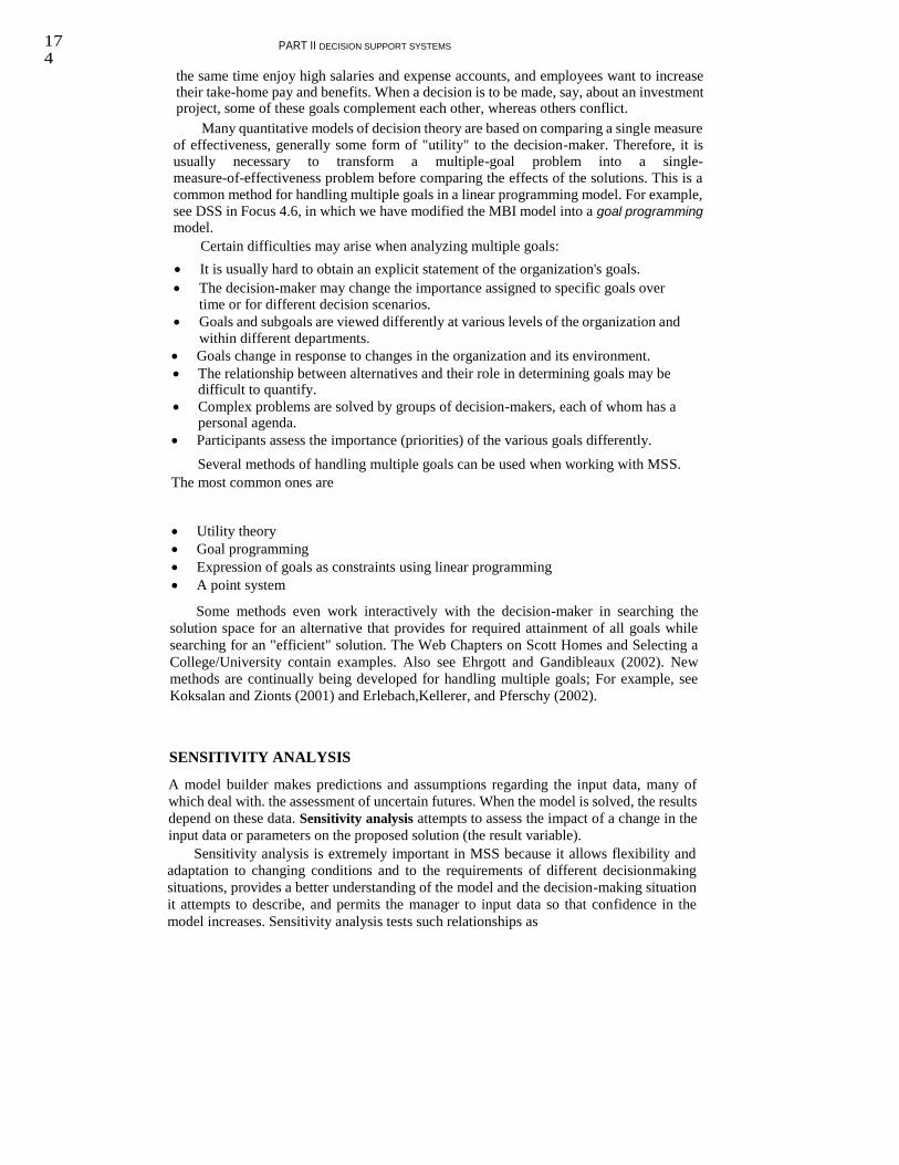
174


the same time enjoy high salaries and expense accounts, and employees want to increase their take-home pay and benefits. When a decision is to be made, say, about an investment project, some of these goals complement each other, whereas others conflict.

Many quantitative models of decision theory are based on comparing a single measure of effectiveness, generally some form of "utility" to the decision-maker. Therefore, it is usually necessary to transform a multiple-goal problem into a single-measure-of-effectiveness problem before comparing the effects of the solutions. This is a common method for handling multiple goals in a linear programming model. For example, see DSS in Focus 4.6, in which we have modified the MBI model into a goal programming

model.

Certain difficulties may arise when analyzing multiple goals:

It is usually hard to obtain an explicit statement of the organization's goals.

The decision-maker may change the importance assigned to specific goals over time or for different decision scenarios.

Goals and subgoals are viewed differently at various levels of the organization and within different departments.

Goals change in response to changes in the organization and its environment.

The relationship between alternatives and their role in determining goals may be difficult to quantify.

Complex problems are solved by groups of decision-makers, each of whom has a personal agenda.

Participants assess the importance (priorities) of the various goals differently.

Several methods of handling multiple goals can be used when working with MSS.

The most common ones are

Utility theory

Goal programming

Expression of goals as constraints using linear programming

A point system

Some methods even work interactively with the decision-maker in searching the

solution space for an alternative that provides for required attainment of all goals while

searching for an "efficient" solution. The Web Chapters on Scott Homes and Selecting a

College/University contain examples. Also see Ehrgott and Gandibleaux (2002). New

methods are continually being developed for handling multiple goals; For example, see

Koksalan and Zionts (2001) and Erlebach,Kellerer, and Pferschy (2002).

SENSITIVITY ANALYSIS

A model builder makes predictions and assumptions regarding the input data, many of

which deal with. the assessment of uncertain futures. When the model is solved, the results

depend on these data. Sensitivity analysis attempts to assess the impact of a change in the

input data or parameters on the proposed solution (the result variable).

Sensitivity analysis is extremely important in MSS because it allows flexibility and

adaptation to changing conditions and to the requirements of different decisionmaking

situations, provides a better understanding of the model and the decision-making situation

it attempts to describe, and permits the manager to input data so that confidence in the

model increases. Sensitivity analysis tests such relationships as


THE GOAL PROGRAMMING MRI MODEL

In a goal programming model, all goals are represented as

constraints that have target values for the left-hand side.

For example, the labor constraint has a target value of

200,000 days. If the target is met, there is no penalty. If we

use more than 200,000 days of labor, we are over our goal,

and there is a penalty for the deviation. If we are under our

goal (i.e., we use less labor than the target amount), there

may also be a penalty, perhaps wages must be paid for no

production. The same is true of the budget constraint. In

this model, we convert the objective of maximizing profit

to a goal of profit meeting or exceeding a target level of $5

million. If we are under our goal, there is a penalty; but if

we are over our goal, there is no penalty. Penalties are

imposed by weights indicating the importance of each of

the multiple objectives and the importance of each being

over or under our goal. The marketing constraints here are

not goals, but required limits.

Profit goal: 8,000 X, + 12,000 X2 - OVERI +

UNDER I '" 5,000,000

Labor goal: 300 Xl + 500 Xz - OVER2 +

UNDER2 '" 200,000

Budget goal: 10,000 Xl + 15,000 Xz - OVER3 +

UNDER,'" 8,000,000

Marketing requirement for CC-7: Xl ~ 100

Marketing requirement for CC-8: Xz ~ 200

The objective is to minimize a weighted sum of the

OVER and UNDER variables. For a particular solution,

the UNDER and OVER variables indicate the amount the

left-hand side of the goal constraint value varies from the

target. Below is a Lingo model and solution. The budget is

right on target (it had the highest weights in the objective).

The profit.is outstanding. We produce 500 units of CC-7

(",Xl)' and 200 units of CC-8 (",Xz)' We .exceeded the $5

million by $1.4 million (= OVERl), which leads to a total

profit of $6.4 million, which is $1.3 million greater than

before. But because OVERz is 50,000, we are using an

additional 50,000 hours of labor. Since the weight in the

objective for OVERz reflects the marginal cost of

obtaining additionallabor, this solution is an improvement

over the standard linear programming one.

Lingo Goalprodmixsimple Model ;

MIN 0 * OVER1 + 1000 * UNDER1 +

50 * OVER2 + 10 * UNDER2 +

100 * OVER3 + 20 * UNDER3 <PROFIT> 8000 * Xl + 12000 * X2 - OVER1 + UNDER1 = 5000000 ; <LABOR>

300 * Xl + 500 * X2 - OVER2 + UNDER2 = 200000 ; <BUDGET> 10000 * xl

+ 15000 * x2 - OVER3 + UNDER3 = 8000000 <MARKET1> Xl >= 100

<MARKET2> X2 >= 200

«< Lingo Goalp~odmixout Solution (Variables only) »>

Variable

OVER1

UNDER1

OVER2

UNDER2

OVER3

UNDER3

Xl X2

Value

1400000.

0.0000000

50000.0

0

0.000000

0

0.000000

0

0.000000

0

500.000

0

200.000

0

Reduced Cost

O.oooooeo 1000.000

0.0000000

60.0000

0

101.500

0

18.5000

0

0.000000

0

0.000000

0


The impact of changes in external (uncontrollable) variables and parameters on outcome variable(s) .

The impact of changes in decision variables on outcome variable(s)

The effect of uncertainty in estimating external variables

The effects of different dependent interactions among variables

The robustness of decisions under changing conditions.

Sensitivity analyses are used for

Revising models to eliminate too large sensitivities

Adding details about sensitive variables or scenarios

Obtaining better estimates of se.isitive external variables

Altering the real-world system to reduce actual sensitivities

Accepting and using the sensitive (and hence vulnerable) real world, leading to the

continuous and close monitoring of actual results

The two types of sensitivity analyses are automatic and trial-and-error.

AUTOMATIC SENSITIVITY ANALYSIS

Automatic sensitivity analysis is performed in standard quantitative model implementa-

tions such as linear programming. For example, it reports the range within which a certain

input variable or parameter value (e.g., unit cost) can vary without making any significant

impact on the proposed solution. Automatic sensitivity analysis is usually limited to one

change at a time, and only for certain variables. However, it is very powerful because of its

ability to establish ranges and limits very fast (and with little or no additional

computational effort). For example, automatic sensitivity analysis is part of the linear

programming (LP) solution report for the MBI Corporation product-mix problem

described earlier. Sensitivity analysis is provided by both Solver and Lindo. If the right-

hand side of the marketing constraint on CC-8 could be decreased by one unit, then the net

profit would increase by $1,333.33. This is valid for the right-hand side decreasing to zero.

For details see Hillier and Lieberman (2003), Taha (2003), and Taylor (2002).

TRIAL AND ERROR

The impact of changes in any variable, or in several variables, can be determined through a

simple trial-and-error approach. You change some input data and solve the problem again.

When the changes are repeated several times, better and better solutions may be

discovered. Such experimentation, which is easy to conduct when using appropriate

modeling software like Excel, has two approaches: what-if analysis and goal seeking.

WHAT-IF ANALYSIS

What-if analysis is structured as What will happen to the solution if an input variable, an

assumption, or a parameter value is changed?

Here are some examples:

What will happen to the total inventory cost if the cost of carrying inventories increases by 10 percent?

What will be the market share if the advertising budget increases by 5 percent?

Assuming the appropriate user interface, it is easy for managers to ask the computer

model these types of questions and get immediate answers. Furthermore, they

43. CHAPTER 4 MODELING AND ANALYSIS 177

Initially, initial sales were 100 growing at 3 percent per quarter yielding an annual net profit of $127. By changing

the initial sales cell to 120 and the sales growth rate to 4 percent, the annual net profit rose to $182.

can perform multiple cases and thereby change the percentage, or any other data in the

question, as desired. All this is done directly, without a computer programmer.

Figure 4.9 shows a spreadsheet example of a what-if query for a cash flow problem.

The user changes the cells containing the initial sales (from 100 to 120) and the sales

growth rate (from 3 percent to 4 percent per quarter). The computer immediately

recomputes the value of the annual net profit cell (from $127 to $182). What-if analysis is

common in expert systems. Users are given the opportunity to change their answers to

some of the system's questions, and a revised recommendation is found.

GOAL SEEKING

Goal seeking analysis calculates the values of the inputs necessary to achieve a desired

level of an output (goal). It represents a backward solution approach. Some examples

of goal seeking are:

What annual R&D budget is needed for an annual growth rate of 15 percent by

2005?

How many nurses are needed to reduce the average waiting time of a patient in the

emergency room to less than 10 minutes?

An example of goal seeking is shown in Figure 4.10. Initially, initial sales were 100

growing at 3 percent per quarter, yielding an annual net profit of $127. By changing the

44.


Annual Year Returns

1lJ.?9~9q 2 $ 130;00 3-SI40:00 4$150:00·

....... " ..........." ....." .....".-.", .. ,.- .. ,.- ...... - ..... .

5 $ 160.00

ilT152.00 .ffj~:~9.

8$ 137.18

ij$i~(j·32· 10 $ 123.80

The goal to be achieved is NPV equal to zero, which determines the internal rate of return (IRR) of this cash flow including the investment. We set the NPV cell to value 0 by changing the interest rate cell. The answer is 38.77059 percent.

initial sales cell to 120 and the sales growth rate to 4 percent, the annual net profit rose to $182.

COMPUTING A BREAK-EVEN POINT

USING GOAL SEEKING

Some modeling software packages can directly compute break-even points, an important

application of goal seeking. This involves determining the value of the decision variables

(e.g., quantity to produce) that generate zero profit. For example, in a financial planning

model in Excel, the internal rate of return is the interest rate that produces a net present

value of zero. In many decision support systems, it can be difficult to conduct sensitivity analysis

because the prewritten routines usually present only a limited opportunity for asking what-if questions. In a DSS, the what-if and the goal-seeking options must be easy to perform.

The goal to be achieved is NPV equal to zero, which determines the internal rate of return (IRR) of this cash flow including the investment. We set the NPV cell to value o by

changing the interest rate cell. The answer is 38.77059 percent.


--_._._----------- 4.11 PROBLEM-SOLVING SEARCH METHODS

SEARCH APPROACHES

When problem-solving, the choice phase involves a search for an appropriate course of

action (among those identified during the design phase) that can solve the problem. There

are several major search approaches, depending on the criteria (or criterion) of choice and

the type of modeling approach used. These search approaches are shown in Figure 4.11.

For normative models, such as mathematical programming-based ones, either an analytical

approach is used or a complete, exhaustive enumeration (comparing the outcomes of all

the alternatives) is applied. For descriptive models, a comparison of a limited number of

alternatives is used, either blindly or by employing heuristics. Usually the results guide the

decision-maker's search.

ANALYTICAL TECHNIQUES

Analytical techniques use mathematical formulas to derive an optimal solution directly or

to predict a certain result. Analytical techniques are used mainly for solving structured

problems, usually of a tactical or operational nature, in areas such as resource allocation or

inventory management. Blind or heuristic search approaches are generally employed to

solve more complex problems.

ALGORITHMS

Analytical techniques may use algorithms to increase the efficiency of the search. An

algorithm is a step-by-step search process (Figure 4.12) for obtaining an optimal solution.

(Note: there may be more than one optimum, so we sayan optimal solution rather than the

optimal solution.) Solutions are generated and tested for possible improvements. An

improvement is made whenever possible, and the new solution is subjected to an

improvement test based on the principle of choice (objective value found). The process

continues until no further improvement is possible. Most mathematical programming

problems are solved by efficient algorithms (see Armstrong, 2001). Web search engines

use algorithms to speed up the search and produce accurate results. Monika Henzinger

developed the algorithms that Google uses in its searches. Google's algorithms are so good

that Yahoo pays $7 million annually to use them (see Patton, 2002/2003).

BLIND SEARCH

In conducting a search, a description of a desired solution may be given. This is called a

goal. A set of possible steps leading from initial conditions to the goal is called the search

steps. Problem-solving is done by searching through the space of possible solutions. The

first of these search methods is blind search. The second is heuristic search, discussed jn

the next section.

Blind search techniques are arbitrary search approaches that are not guided. There are two types of blind searches: a complete enumeration, for which all the alternatives are considered and therefore an optimal solution is discovered; and an incomplete, partial search, which continues until a good-enough solutionis found. The latter is a form of suboptimization.

There are practical limits on the amount of time and computer storage available for blind searches. In principle, blind search methods can eventually find an optional

45.

tt ~ Cllll s: III c: Ql . Cl

C Ql Ql 0>"0 ::l a B B E';:; ~ 0

'., c :J co co ro ~ (J Ql

"0 E E ~t-CJ "0

gj iH3 0

en .;:; "B- 0

0. !Ilro (!J

a a

0 •.• c: c: . c:Qll!1 QlE,Q .c:Qllll »lIl >00 0. ••. 0. o Ill. en.~ .!Il

]

~ ••. ro ro Ql O-lIl

ui Ql .c:.c: (J (J ••.

ro ro 0 Ql ••. eno.

0. ro

180

c o . . - .c: .2~ 00 III c c: Ql Ql"O .c:o ~ 0 o..Cl o III •... -

en


Yes

Improve solution.

Generate a new

proposed solution.

solution in most search situations, and in some situations the scope of the search can be

limited; however, the method is not practical for solving very large problems because too

many solutions must be examined before an optimal solution is found.

HEURISTIC SEARCH

For many applications, it is possible to find rules to guide the search process and reduce the

amount of necessary computations. This is done by heuristic search methods, which we

describe next.

4.12 HEURISTIC PROGRAMMING

The determination of optimal solutions to some complex decision problems could involve

a prohibitive amount of time and cost or may even be impossible. Alternatively, the

simulation approach (Section 4.13) maybe lengthy, complex, inappropriate, and even

inaccurate. Under these conditions it is sometimes possible to obtain satisfactory solutions

more quickly and less expensively by using heuristics.

Heuristics (from the Greek word for discovery) are decision rules governinghow a

.' problem should be solved. Usually, heuristics are developed on the basis of a solid, rig-

orous analysis of the problem, sometimes involving carefully designed experimentation. In

contrast, guidelines are usually developed as a result of a trial-and-error experience. Some

heuristics are derived from guidelines. Heuristic searches (or programming)are

step-by-step procedures (like algorithms) that are repeated until a satisfactory solution is

found (unlike algorithms). In practice, such a search is much faster and cheaper than a

blind search, and the solutions can be very close to the best ones. In fact, problems that

theoretically can be solved to optimality (but with a very long solution time) are in practice

sometimes solved by heuristics, which can guarantee

46. 112


Sequence jobs through a machine

Purchase stocks

Do the jobs that require the least time first. If a price-to-earnings ratio exceeds 10, do not buy the stock.

Do not use the freeway between 8 and 9 a.m.

Consider only projects with estimated payback

periods of less than 2 years.

Buy only in a good neighborhood, but buy only in the lower price range.

Travel

Capital investment in high-tech projects

Purchase of a house

a solution within a few percent of the optimal objective value. For details and advances, see

Glover and Kochenberger (2001). Examples of heuristics are given in Table 4.6. Decision-makers use heuristics or rules of thumb for many reasons, some more reasonable

than others. For example, decision-makers may use a heuristic if they do not know the best way

to solve a problem or if optimization techniques have not yet been developed. A decision-maker

might not be able to obtain all the information necessary, or the cost of obtaining the

information or developing a complex model may be too high. This was done in the Cameron

and Barkley Company's Web-based DSS for reducing inventories and improving overall

service performance, described in DSS in Action 3.2; see Cohen, Kelly, and Medagli (2001). The heuristic process can be described as developing rules to help solve complex problems

(or intermediate subproblems to discover how to set up subproblems for final solution by

finding the most promising paths in the search for solutions), finding ways to retrieve and

interpret information on the fly, and then developing methods that lead to a computational

algorithm or general solution. Although heuristics are employed primarily for solving ill-structured problems, they can

also be used to provide satisfactory solutions to certain complex, wellstructured problems much

more quickly and cheaply than optimization algorithms (e.g., large-scale combinatorial

problems with many potential solutions to explore) (Sun et aI., 1998). The main difficulty in

using heuristics is that they are not as general as algorithms. Therefore, they can normally be

used only for the specific situation for which they were intended. Another problem with

heuristics is that they may produce a poor solution. Heuristics are often stated like algorithms.

They can be step-by-step procedures for solving a problem, but there is no guarantee that an

optimal solution will be found.

It is critical to realize that heuristics provide time-pressured managers and other

professionals with a simple way of dealing with a complex world, producing correct

or partially correct judgments more often than not. In addition, it may be inevitable

that humans will adopt some way of simplifying decisions. The only drawback is

that individuals frequently adopt ... heuristics without being aware of them.

(Bazerman, 2001)

Heuristic programming is the approach of using heuristics to arrive at feasible and "good

enough" solutions to some complex problems. Good enough is usually in the range of 90-99.9

percent of the objective value of an optimal solution. Heuristics can be quantitative, and so can

playa major role in the DSS model base, where heuristics were used to solve a complex integer

programming problem. They can also be qualitative, and then can playa major role in providing

knowledge to expert systems.


ANALYSIS

183

METHODOLOGY

Heuristic thinking does not necessarily proceed in a direct manner. It involves searching,

learning, evaluating, judging, and then re-searching, relearning, and reappraising as

exploring and probing take places'Ihe knowledge gained from success or failure at some

point is fed back/to and modifies the search process. It is usually necessary either to

redefine the objectives or the problem or tosolve related or simplified problems before the primary one can be solved. .

Tabu search heuristics (Glover and Kochenberger, 2001) are based on intelligent

search strategies to reduce the search for high-quality solutions in computer problem-

solving. Essentially, the method "remembers" what high-quality and low-quality solutions

it has found and tries to move toward other high-quality solutions and away from the

low-quality ones. The tabu search methodology has proved successful in efficiently

solving many large-scale combinatorial problems (e.g., the fixed-charge transportation

problem; see Sun et al., 1998). Tabu search heuristics were part of Bourjolly et al.'s (2001)

method for allocating cell telephone frequencies in Canada.

Genetic algorithms (Reeves and Rowe, 2002; Sarker et al., 2002) start with a set of

randomly generated solutions and recombine pairs of them at random to produce offspring

(modeled on the evolution process). Only the best offspring and parents are kept to produce

the next generation. Random mutations may also be introduced. Some new applications are

described by Ursem, Filipic and Krink (2002) for greenhouse control, and by Borgulya

(2002) for machine scheduling. Genetic algorithms are described in depth in a later

chapter.

WHEN TO USE HEURISTICS

Heuristic application is appropriate in the following situations:

The input data are inexact or limited.

Reality is so complex that optimization models cannot be used.

A reliable exact algorithm is not available.

Complex problems are not economical for optimization or simulation or consume excessive computation time.

It is possible to improve the efficiency of the optimization process (e.g., by pro-ducing good starting solutions).

Symbolic rather than numerical processing is involved (as in expert systems).

Quick decisions must be made and computerization is not feasible (some heuristics do not require computers).

ADVANTAGES AND LIMITATIONS OF HEURISTICS

The major advantages of heuristics are the following:

They are simple to understand and therefore easier to implement and explain.

They help train people to be creative and develop heuristics for other problems.

They save formulation time.

They save computer programming and storage requirements.

They save computational time and thus real time in decision-making. Some problems are so complex that they can be solved only with heuristics.

They often produce multiple acceptable solutions.

Usually it is possible to state a theoretical or empirical measure of the solution quality (e.g., how close the solution's objective value is to an optimal one, even though the optimal value is unknown).


They can incorporate intelligence to guide the search (e.g., tabu search). Such expertise

may be problem specific or based on an expert's opinions embedded in an expert system

or search mechanism.

It is possible to apply efficient heuristics to models that could be solved with

mathematical programming. Sometimes heuristics are the preferred method, and other

times heuristic solutions are used as initial solutions for mathematical programming

methods.

The primary limitations of heuristics are the following:

An optimal solution cannot be guaranteed. Sometimes the bound on theobjective value

is very bad.

There may be too many exceptions to the rules.

Sequential decision choices may fail to anticipate the future consequences of each choice.

The interdependencies of one part of a system can sometimes have a profound

influence on the whole system.

Heuristic algorithms that function like algorithms but without a guarantee of optimality can

be classified as follows (Camm and Evans, 2000):

Construction heuristics. These methods build a feasible solution by adding components

one at a time until a feasible solution is obtained. For example, ina traveling salesperson

problem, always visit the next unvisited city that is closest.

Improvement heuristics. These methods start with a feasible solution and attempt to

successively improve on it. For example, in a traveling salesperson solution, attempt to

swap two cities.

Mathematical programming. This method is applied to less constrained (relaxed) models

in the hope of obtaining information about an optimum to the original one. This

technique is often used in integer optimization.

Decomposition. This approach involves solving a problem in stages. In the P&G Web

Chapter, the distribution problem was solved and then used in solving the

product-strategy problem.

Partitioning. This method involves dividing a problem up into smaller, SOlvable pieces

and then reassembling the solutions to the pieces. This technique can be applied to large

traveling salesperson problems. The country can be divided into four regions, each

problem solved, and then the solutions connected together.

Vehicle routing has benefited from the development and use of efficient.heuristics

(e.g., Applegate et al., 2002; Belenguer, Martinez, and Mota, 2000; FOUlds and Thachenkary,

2001; LaPorte et aI., 2002; Liu andShen, 1999; Gendreau et al., 1999), as has university course,

classroom, and faculty scheduling (see Foulds and Johnson, 2000). Karaboga and Pham (1999)

and Glover and Kochenberger (2001) discuss modern heuristic methods (tabu search, genetic

algorithms, and simulated annealing). Also see Nance and Sargent (2002).

--- ,----.---"------'----'----'----'-----'---

4.13 SIMULATION

To simulate means to assume the appearance ofthe characteristics of reality. In MSS, simulation

is a technique for conducting experiments (e.g., what-if analyses) with a computer on a model of

a management system.

CHAPTER 4 MODELING AND ANALYSIS

185

Typically there is some randomness in the real decision-making situation. Because DSS

deals with semistructured or unstructured situations, reality is complex, which may not be

easily represented by optimization or other models but can often be handled by simulation.

Simulation is one of the most commonly used DSS methods.

MAJOR CHARACTERISTICS OF SIMULATION

Simulation is not strictly a type of model; models generally represent reality, whereas

simulation typically imitates it. In a practical sense, there are fewer simplifications of

reality in simulation models than in other models. In addition, simulation is a technique for

conducting experiments. Therefore, it involves testing specific values of the decision or

uncontrollable variables in the model and observing the impact on the output variables. In

the Opening Vignette, the DuPont decision-makers had initially chosen to purchase more

rail cars, whereas an alternative involving better scheduling of the existing cars was

developed, tested, found to have excess capacity, and saved money.

Simulation is a descriptive rather than a normative method. There is no automatic

search for an optimal solution. Instead, a simulation model describes or predicts the

characteristics of a given system under different conditions. Once the values of the

characteristics are computed, the best of several alternatives can be selected. Thesim-

ulation process usually repeats an experiment many, many times to obtain an estimate (and

a variance) of the overall effect of certainactions. For most situations, a computer

simulation is appropriate, but there are some well-known manual simulations (e.g., a city

police department simulated its patrol car scheduling with a carnival game wheel).

Finally, simulation is normally used only when a problem is too complex to be treated

by numerical optimization techniques. Complexity here means either that the problem

cannot be formulated for optimization (e.g., because the assumptions do not hold), the

formulation is too large, there are too many interactions among the variables, or the

problem is stochastic in nature (exhibits risk or uncertainty). Designing and testing a new

model of an automobile is extremely complex. That is one reason why General Motors

utilizes simulation throughout the entire design process (see Gallagher, 2002; Gareiss,

2002; Witzerman, 2001). The success of General Motors may have prompted

Daimler-Chrysler to move in this direction. By 2005, its Digital Factory, which utilizes

simulation and visualization tools, will have helped to design, build, and retrofit all of its

plants (see Hoffman, 2002).

ADVANTAGES OF SIMULATION

Simulation is used in MSS for the following reasons:

The theory is fairly straightforward. A great amount of time compression can be attained, quickly giving the manager

some feel as to the long-term (1- to 10"year) effects of many policies.

Simulation is descriptive rather than normative. This allows the manager to pose

what-if questions. Managers can use a trial-and-error approach to problemsolving

and can do so faster, cheaper,more accurately, and with less risk (see the

opening vignette). The manager can experiment to determine which decision variables and

which parts of the environment are really important, and with different alterna-

tives. An accurate simulation model requires an intimate knowledge of the problem,

thus forcing the MSS builder to constantly interact with the manager. This is

desirable for DSS development because the developer and manager both gain a


better understanding of the problem and the potential decisions available (Eldabi et al., 1999) (see the opening vignette).

The model is built from the manager's perspective.

The simulation model is built for one particular problem and typically cannot solve

any other problem. Thus, no generalized understanding is required of the manager;

every component in the model corresponds to part of the real system.

Simulation can handle an extremely wide variety of problem types, such as inventory and staffing, as well as higher-level managerial functions, such as long-range planning.

Simulation generally can include the real complexities of problems; simplifications

are not necessary. For example, simulation can use real probability distributions rather than approximate theoretical distributions. .

Simulation automatically produces many important performance measures.

Simulation is often the only DSS modeling method that can readily handle rela-tively unstructured problems.

There are some relatively easy-to-use (Monte Carlo) simulation packages. These include add-in spreadsheet packages (@Risk), the influence diagram software mentioned earlier, Java-based (and other Web development) packages, and the

visual interactive simulation systems to be discussed shortly.

DISADVANTACES OF SIMULATION

The primary disadvantages of simulation are the following:

An optimal solution cannot be guaranteed, but relatively good ones are generally found.

Simulation model construction can be a slow and costly process, although newer modeling systems are easier to use than ever.

Solutions and inferences from a simulation study are usually not transferable to other problems because the model incorporates unique problem factors.

Simulation is sometimes so easy to explain to managers that analytic methods are often overlooked.

Simulation software sometimes requires special skills because of the complexity of the formal solution method.

THE METHODOLOCY OF SIMULATION

Simulation involves setting up a model of a real system and conducting repetitive experiments on it. The methodology consists of the steps shown in Figure 4.13.

PROBLEM DEFINITION

The real-world problem is examined and classified. Here we specify why a simulation approach is appropriate. The system's boundaries, environment, and other such aspects of problem clarification are handled here.

CONSTRUCTION OF THE SIMULATION MODEL

This step involves determination of the variables and their relationships, and data gath-ering. Often the process is described by a flowchart, and then a computer program is written.

TESTINC AND VALIDATINC THE MODEL

The simulation model must properly represent the system under study. Testing and val-idation ensure this.


DESIGN OF THE EXPERIMENT

Once the model has been proven valid, an experiment is designed. Determining how long

to run the simulation is part.of this step. There are two important and conflicting

objectives: accuracy and cost. It is also prudent to identify typical (mean and median cases

for random variables), best-case (e.g., low-cost, high-revenue), and worst-case (e.g.,

high-cost, low-revenue) scenarios. These help establish the ranges of the decision

variables and environment in which to work and also assist in debugging the simulation

model.

CONDUCTING THE EXPERIMENT

Conducting the experiment involves issues ranging from random-number generation to

result presentation.

EVA.LUATING THE RESULTS

The results must be interpreted. In addition to standard statistical tools, sensitivity

analyses can also be used.

IMPLEMENTATION

The implementation of simulation results involves the same issues as any other imple-

mentation. However, the chances of success are better because the manager is usually

more involved in the simulation process than with other models. Higher levels of man-

agerial involvement generally lead to higher levels of implementation success.

Many simulation packages are Web ready. They typically are developed along the

lines of the DSS architecture shown in Figure 3.1, where a user connects to the main server

through a Web browser. This server connects to optimization servers, database servers,

and they in turn may connect to data warehouses, which populate the models. For example,

see Pooley and Wilcox (2000) for a description of a Java-based simulation system. Also

see major vendors' Web sites.

TYPES OF SIMULATION

PROBABILISTIC SIMULATION

In probabilistic simulation, one or more of the independent variables (e.g., the demand in

an inventory problem) are probabilistic. They follow certain probability distribu-

tions,which can be either discrete distributions or continuous distributions.

47. 188 PART II DECISION SUPPORT SYSTEMS

Daily Demand

5

6

7 8 9

Discrete Probability

.10

.15

.30

.25

. 20

Continuous Probabiliiy:

Daily demand is normally distributed with a mean of7 and a standard deviation ofL2 .

Discrete distributions involve a situation with a limited nuniber of events (or

variables) that can take on only a finite number of values. Continuous distributions are situations with unlimited numbers of possible

events that follow density functions, such as the normaldistribution;

The two types of distributions are shown in Table 4.7.Probabilistic simulation is conducted.with the aid of a technique called Monte Carlo, which was used in the opening vignette situation.

TIME-DEPENDENT VERSUS

TIME-INDEPENDENT SIMULATION Time-independent refers to a situation in which it is not important-to know exactly when

the event occurred. For example, we may know that the demand for a certain product is

three units per day, but we do not care when during the day the item is demanded. In some

situations, time may not be a factor in the simulation at all, such as in steady-state plant

control design (Boswell, 1999). On the other hand, in waiting-line problems applicable to

e-commerce, it is important to know the precise time of arrival (to know whether the

customer will have to wait). This is a time-dependent situation.

SIMULATION SOFTWARE ) .

There are hundreds of simulation packages for a variety of decision-making situations. Most run as Web-based systems (see Dembo et aI., 2000). PC software packages include

Analytica (Lumina Decision Systems, lumina.com), and the Excel add-ins Crystal Ball

(Decisioneering, decisioneering.com) and @Risk (Palisade Software, palisade.com).

Web-based systems include WebGPSS (GPSS, webgpss.hk-r.se), SIMUL8 (SIMUL8

Corporation, SIMUL8.com), and Silk (ThreadTec,· Inc., threadtec.com).

VISUAL·SIMULATION The graphical display of computerized results, which may include animation, is one of the

more successful developments in computer-human interaction and problemsolving. We

describe this in the next section.

OBJECT-ORIENTED SIMULATION There have been some advances in thearea of developing simulation models using the

object-oriented approach (e.g., Yun and Choi, 1999). Yun and Choi (1999) describe an

object-oriented simulation model for container-terminal operation analysis. Each piece of

equipment at the terminal maps into an object representation in the simulation model.

SIMPROCESS (CACI Products Company, caciasl.com) is an object-

CHAPTER 4 MODELING AND ANALYSIS

189

oriented process modeling tool that lets the user create a simulation model with screen-based

objects. Unified modeling language (UML) is a modeling tool that was designed for

object-oriented and object-based systems and applications. Since UMLis object-oriented, it

could be used in practice for modeling complex, real-time systems. UML is particularly well

suited for modeling. A real-time system is a software system that maintains an ongoing, timely

interaction with its. environment; examples include many DSS and information and

communication systems (Selic, 1999).

SIMULATION EXAMPLE

We show an example of a spreadsheet-based economic order quantity simulation model and a

spreadsheet simulation model for evaluating a simple cash-flow problem ina Web Chapter. DSS

in Action 4.7 describes a case study of applying simulation to IT network design. CACI

Products Company now provides COMNET III, a simulation system specifically for analyzing

these types of IT network design problems. Saltzman and Mehrotra (2001) used a simulation

approach to analyze a call center. Jovanovic (2002) determines how to schedule tasks in

distributed systems via simulation. This is important when managing grid computer networks.

Dronzek (2001) used simulation to

improve critical care in a military hospital. .

He analyzed proposed changes in a health care system using simulation modeling to

determine the impact of potential changes without disrupting the established process of care or

disturbing staff, patients, or the facility. Credit Suisse First Boston uses an ASP simulation

system to predict the risk and-reward potential of investments (see Dembo et al., 2000}.General

Motors (see Gallager, 2002; Gareiss, 2002; Witzerman,2001) delays constructing physical

models of automobiles until late in the design process, since simulation is cheaper and produces

more accurate results in testing new products. This includes crash tests and wind tunnel tests.

Witzerman (2001) describes how GM's paint shop robots are simulated for improved

performance. These tools are very effective and have led to major improvements. It now takes

only 18 months to develop a new vehicle, down from 48 months. Engineering productivity is

way up, as is quality. Also see Marchant (2002).

-~~~------- 4.14 VISUAL IN.TERACTIVE MODELING AND VISUAL INTERACTIVE SIMULATION

CONVENTIONALS IMU LATION

Simulation is a well-established, useful method for gaining insight into complex MSS

situations. However, simulation does not usually allow decision-makers to see how a solution to

a complex problem evolves over. (compressed) time, nor can they interact with it. Simulation

generally reports statistical results at the end of a set of experiments. Decision-makers are thus

not an integral part of simulation development and experimentation, and their experience and

judgment cannot be used directly in the study.If the simulation results do not match the intuition

or judgment of the decisionmaker, a confidence gap in the use of the model occurs. One of the most exciting developments in computer graphics is visual interactive

modeling (VIM) (see DSS in Action 4.8). The technique has been.used with great success for

DSS in the area of operations management. Decision-makers who used VIM in

48. 190


PACIFIC BELL USES SIMULATION TO

DESIGN AN IT NETWORK

Decision support simulation software for networks and

networked applications can be used to experiment with

multiple what-if scenarios. Then IT can determine a best

solution before making blind commitments or sinking

resources into large projects without a thorough under-

standing of the expected outcome. Simulations help IT

determine how the infrastructure would react to a given

scenario, such as increased network traffic, new transport

technologies, topology changes, and new prioritized

applications like ERP and voice-over Internet protocol (IP).

The value of a decision-support tool is its ability to deliver

reliable, timely, and verifiable data about result variables,

leading to confident, resourcesaving decisions-critical

during initial IT system design and implementation, when

trade-offs can be weighed and cost considerations

examined before committing heavily to a project.

Pacific Bell, a subsidiary of SBC Communications,

Inc. (SBC), collaborated with a large government agency

in southern California to design a network to support more

than 80,000 employees at hundreds of sites. Throughout the southern California project, SBC and the government

utilized IT DecisionGuru, a modeling and simulation tool

from MIL 3 Inc. (Washington, D.C).

The challenge for the SBClgovernment team was to

design a network backbone to link thousands of nodes at

every site into a network capable of supporting data, video,

and voice and to support future growth. The design team

first built a baseline model of projected "typical" network

activity. Then it used its simulation software to explore the relative performance gains offered by various architecture

options. This process enabled the design team to visualize

all relevant network performance indicators.

After running several simulations, it was determined

that a network consisting of only ATM OC-J links would

have very low utilization. While perfectly acceptable from

a performance perspective, it would be very expensive.

But a network with only Tl links performs poorly at a

lower cost. The best solution combined the cost efficiency

ofTllines with the bandwidth of ATM links, as the

simulation indicated. This middleof-the-road strategy

saved a lot of money and avoided potentially costly

impacts from poor performance.

The most critical issue was the sizing of the dedicated

wide area network (WAN) links. There was a trade-off

between overprovisioned service, for which excess capacity would cost hundreds of thousands of dollars

unnecessarily, and underprovisioning, which could cause

unacceptably poor network performance. By simulating

the key decision elements, the SBClgovernment team

designed an efficient architecture to handle anticipated

bandwidth needs at an acceptable cost. Without sacrificing service levels, the government reduced its expected WAN

costs by more than 25 percent, translating into millions of

dollars saved per year.

SBC also benefited in much the same way that any

internal IT organization can benefit from simulation. It

built credibility with business decision-makers by pro-

viding quantifiable data to support its recommendations,

making government decision-makers much more

comfortable that SBC could deliver the service levels it promised.

Source: Based on S. Toborg and M. Cohen, "Benefits and Savings Accrue with Simulation," Communications News, Vol. 36, No.9, Sept. 1999, pp. 34-36.

/

their decision-making were surveyed and found to have a high level of support for and interest in

these models (Bell et aI., 1999). This technique has several names and variations, including visual

interactive problem-solving, visual interactive modeling, and visual interactive simulation.

Visual interactive modeling uses computer graphic displays to present the impact of different

managerial decisions. It differs from regular graphics in that the user can adjust the decision-making

process and see the results of the intervention. A visual model is a graphic used as an integral part of

decision-making or problem-solving, not just as a communication device. The VIM displays the

effect of different decisions in graphic form on a computer screen, as was done through the GIS in the

P&G supply chain redesign through optimization (Web Chapter). Some people respond better to

graphical displays, and this


VISUAL INTERACTIVE SIMULATION:

U.S. ARMY HOSPITAL USES ANIMATED

SIMULATION OF A FAMILY PRACTICE CLINIC

The u.s. Army Hospital in Heidelberg, Germany, used

animated simulation to develop viable alternatives for

their family practice clinic. The clinic was attempting to

examine different staffing alternatives, determine the best

patient and staff flow scheme, and increase productivity to

provide sufficient capacity. An animated simulation

model was developed. The current environment, as

represented by the status quo model, could not provide the

needed capacity of outpatient visits. Alternative models

were developed, two of which were good possibilities.

The two alternative models, an all-physician model (the

"physician model") and a combination model with both

physicians and nonphysician providers (the "combo

model"), were run and compared, and neither could

handle the patient load. A process change in parallel

patient screening was developed to increase patient

throughput and to increase capacity. Then both models

could meet clinic capacity requirements, both in the newly

planned clinic and in the current one. Based on the

simulation, the physician and combo models were

selected for the health care operation in a phased-in plan

from the former to the latter.

The simulation gave the decision-makers insight into

provider and support staff use rates, down time, and

small but significant process improvements. The all-

physician model was recommended as a short-term

arrangement after considering cost, supervisory issues,

and provider availability. Changes at the clinic were to

take place in the near future, and phasing in the non-

physician providers would take some time.

Although the physician model was selected as a

short-term arrangement to meet the needs of the com-

munity and health care system, the simulation model

showed that much more work and evaluation of patient

wait times had to be conducted to decrease the wait for

customers. Management had determined the number of

physicians and staff members needed to meet patient

capacity needs, the necessary size of the waiting area, the

necessary provider scheduling changes, and the process

changes necessary to meet the capacity requirement,

patient expectations, and organizational goals via

simulation. The move to the renovated area was successful

and had the additional results of impaneling the

beneficiaries in the community. A migration plan was

adopted based on further simulation runs.

Source: Adapted from Ledlow et al. (1999).

type of interaction can help managers learn about the decision-making situation. For example,

Swisher et al. (2001) applied an object-oriented visual simulation to examining the functioning of a

physician clinic environment within a physician network to provide high-quality, cost-effective

healthcare in a family practice. The simulation system identified the most important input factors that

significantly affected performance. These inputs, when properly managed, led to lower costs and

higher service levels.

VIM can represent a static or a dynamic system. Static models display a visual image of the

result ofone decision alternative at a time. Dynamic models display systems that evolve over time,

and the evolution is represented by animation. A snapshot example of a generated animated display

of traffic at an intersection, from the Orca Visual Simulation Environment (Orca Computer Inc.,

Blacksburg, Virginia, orcacomputer.corn), is shown in Figure 4.14. The Orca Web site shows

several animations that were generated by its simulation system.

VISUAL INTERACTIVE SIMULATION

Visual simulation is one of the most exciting dynamic VIMs. It is a very important DSS technique

because simulation is a major approach in problem-solving. Visual interactive simulation (VIS)

allows the end user to watch the progress of the simulation model in an animated form on graphics

displays.


Courtesy of Orca Computer, Inc., Blacksburg, VA

The basic philosophy of VIS is that decision-makers can interact with the simulated

model and watch the results develop over time (see the Web demos at Orca Computer Inc.,

orcacomputer.com). The user can try different decision strategies online. Enhanced

learning, both about the problem and about the impact of the alternatives tested, can and

does occur. Decision-makers can also contribute. to model validation. They will have more

confidence in its use because of their own participation in its development and use. They

are also in a position to use their knowledge and experience to interact with the model to

explore alternative strategies. Ledlow et al. (1999) describe how the U.S. Army Hospital in

Heidelberg, Germany, used animated simulation to develop viable alternatives for its

family practice clinic (see DSS in Action 4.8).

Animated VIS software systems are provided by Orca Computer, 'Inc., GPSS/PC

(Minuteman Software), and VisSim (Visual Solutions). The latest visual simulation

technology is coupled with the concept of virtual reality, where an artificial world is

created for a number of purposes, from training to entertainment to viewing data in an

artificial landscape. For example, Harris Corp. has developed a visual interactive

simulation system for the U.S. military. The system lets ground troops gain familiarity with

terrain or a city so that they can very quickly orient themselves. It also is used by pilots to

gain familiarity with targets by simulating attack runs. The software includes GIS

coordinates. (CNN Television Report, Nov. 16,2002.)


ANALYSIS

193

VISUAL INTERACTIVE MODELS AND DSS

VIM in DSS has been used in several operations management decisions. The method

consists of priming a visual interactive model of a plant (or company) with its current

status. The model then runs rapidly on a computer, allowing management to observe how a

plant is likely to operate in the future.

Waiting-line management (queuing) is a good example of VIM. Such a DSS usually

computes several measures of performance (e.g., waiting time in the system) for the

various decision alternatives. Complex waiting-line problems require simulation. VIM can

display the size of the waiting line as it changes during the simulation runs and can also

graphically present the answers to what-if questions regarding changes in input variables. The VIM approach can also be used in conjunction with artificial intelligence.

Integration of the two techniques adds several capabilities that range from the ability to

build systems graphically to learning about the dynamics of the system. High-speed

parallel computers such as those made by Silicon Graphics Inc. and Hewlett-Packard make

large-scale, complex, animated simulations feasible in real time (the movie Toy Story and

its sequel were essentially long VIMs). The grid computing paradigm may help in

large-scale simulations.

General-purpose commercial dynamic VIM software is readily available. For

information about simulation software, visual and otherwise, see The IMAGE Society Inc.

Web site (public.asu.edu), the Society for Computer Simulation International Web site

(scs.org), and the annual software surveys at the OR/MS Today Web site (lionhrtpu b.com/

orms/).

--- ~~ ..-----------

4.15 QUANTITATIVE SOFTWARE PACKAGES

Some DSS tools offer several built-in subroutines for constructing quantitative models in

areas such as statistics, financial analysis, accounting, and management science. These

models can be activated by a single command, such as

MOVAVG. This function calculates a moving average estimated forecast of a time

series of data. It might be embedded in a production planning model to generate

demand. NPV. This function calculates the net present value of a series of future cash

flows for a given interest rate. It could be part of a make-versus-buy model.

OLAP systems are essentially a collection of optimization, simulation, statistical, and

artificial intelligence packages that access large amounts of data for analysis. (For

example, Oracle Financials Suite provides business intelligence and risk management

applications; see Ferguson, 2002.) In addition, many DSS tools can easily interface with

powerful standard quantitative stand-alone software packages. A DSS builder can increase

his or her productivity by using quantitative software packages (preprogrammed models

sometimes called "ready-made") rather than "reinventing the wheel." Some of these

models are building blocks of other quantitative models. For example, a regression model

can be part of a forecasting model that supports a linear programming planning model (as

in the P&G Web Chapter and IMERYS Case Application 4.1). Thus, a complicated model

can easily be integrated with many sets of data. The Lingo modeling language described

earlier for optimization problems can be

194

PART ll DECISION SUPPORT SYSTEMS

designed with a SET definition section and a DATA section. The sets and data can be fed

from a database, while the actual Lingo model lines do not explicitly state any dimension

or data aspects. While spreadsheets have the same capability, data must be carefully

inserted. For a comprehensive resource directory of these types of systems, see the ORiMS

Today Web site (lionhrtpub.com/orms/). Since the Web has promoted the widespread use

of modeling, optimization, simulation, and related techniques, we list a sampling of Web

impacts on these areas, and vice versa, in Table 4.8.

Data mining tools are utilized for customer segmentation analysis. These tools

automate much of the tedious nature of using standard optimization packages by providing

convenient and powerful ways to analyze sales. These customer analytic tools are

available from Cognos, Inc. (cognos.com), DigiMine Inc. (digimine.com), Hyperion

Solutions Corp. (hyperion.com), IBM (ibm.com), Informatica Corp. (informatica. com),

Megaputer Intelligence, Inc. (megaputer.com), Oracle Corp. (oracle.com), and Teradata

(teradata.com). (See Pallatto, 2003.)

These tools are improving in capability, portability, and usability almost daily.

Similar to developments in enterprise resource planning systems for operational

applications, new OLAP-type ADP (Analytical Development Platforms) plug-anddevelop

capabilities enable developers to build sophisticated applications with a unique look, feel,

and functionality in a few days or weeks. Vendors include AlphaBlox, Proclarity, and

Business Objects (see Callaghan, 2003). Object models are automatically created in

graphical, configurable, Web-ready components. See Eckerson (2003) and Fourer and

Goux (200~) for details. Finally, Hossein Arsham (2003a, 2003b) maintains an extensive

bibliography on decision-making tools and decision sciences resources.

STATISTICAL PACKAGES

Several statistical functions are built into various DSS tools, such as mean, median,

variance, standard deviation, kurtosis, t-test, chi-square, various types of regression

(linear, polynomial, and stepwise) correlations, forecasting, and analysis of variance.

Web-based statistics packages include STATLib (lib.stat.cmu.edu), StatPages.net

(statpages.net), StatPoint Internet Statistical Computing Center (sgorp.corn/ on-Iine

.computing.htm), and SticiGui (stat.Berkeley.edu/ -stark/SticiGui/).

Regression analysis is a powerful statistical curve-fitting technique. An example of an

SPSS run that quickly analyzed a set of data appears in a Web Chapter. The run was

triggered with a single click of a button, the results were clearly delineated in the report,

and the report was automatically formatted. These features can readily enhance a DSS

developer's capabilities.

More power can be obtained from stand-alone statistical packages, some embedded in

OLAP, which can readily interface with spreadsheets (Excel). Typical packages include

SPSS and Systat (SPSS Inc., Chicago, Illinois, spss.com), Minitab (Minitab Inc., State

College, Pennsylvania, minitab.com), SAS (SAS Institute Inc., Cary, North Carolina,

sas.com), and TSP (TSP International, Palo Alto California, tspintl.com). StatPac Inc.

(statpac.com, Minneapolis, Minnesota) includes survey analysis software in itsStatPac

package. Most spreadsheets also contain sophisticated statistical functions and routines.

Statistical software is now considered more a decision-making tool than a sophisti-

cated analytical tool in the decision-making process. It is even embedded in Web-ready

data mining and OLAP tools, and so the user is unaware that sophisticated statistical

methods are being used. This subtle change in the user's focus has occurred because of the

maturity of well-accepted technology and the low cost and high performance of

computers. This has clearly led to a greater acceptance of statistical methodologies.

49. CHAPTER 4 MODElING AND ANALYSIS 195

Modeling Topic

Models

Mathematical Programming (

Optimization)

Heuristics

Simulation

Model Management Systems

Web Impacts

Application servers provide access to

models and their solution methods in a

consistent, friendly, graphical user

interface

Provides for a direct mechanism to

query solutions

Provides a channel to integrate models and

models with data

Provides a consistent communication

channel

New programming languages and

systems Intranets and extranets influence the

use of models in supply chain management,

customer relationship management and

revenue management

Proliferation of model use throughout

organizations-makes enterprisewide

systems like SCM and CRM feasible

and practical

Access to information about models

Makes models usable for e-commerce

settings

All of the above

Access to models and solution methods

implemented as Java applets and other

Web development systems

Use of models by untrained managers

because they are so easy to use

Access to Web-based AI tools to

suggest models and solution methods in DSS

Access to information about models

All of the above

All of the above Improved visualization and delivery

of results

Distributed processing

Access to Web-based programming

tools, AI methods, and application

servers that perform model

management New Web-based model management

systems

Impacts on the Web

Describes the Internet/Web, intranet and

extranet structures as networks

Describes how to optimize Web

performance-sites and message

routing from site to site and

bandwidth allocation

Provides a means to analyze

e-commerce (transactions and other

processes can be analyzed) to

determine effectiveness and

efficiency Model base application servers Models

to evaluate tradeoffs among service

levels and types Forecasting models

predict viability of hardware and

software choices Forecasuag-models

predict network performance and

e-commerce activity

Improved component and other

hardware selection

All of the above

Improved infrastructure design and

updates

Traveling salesman model (vehicle

routing) solutions improve

dynamic message routing; also

improved integrated circuit and

circuit board design

Internet communication readily

enables grid computing

All of the above Establish rules rather than optimize to

determine how to structure networks and

message routing Simulation of difficult,

probabilistic

models lead to better performance

Simulation of Web traffic Simulation of Web site activities for

better e-commerce performance

AI-based methods for model

management have improved Web

performance by improving the

effectiveness and efficiency of the network infrastructure .


MANAGEMENT SCIENCE (ANALYTICAL

MODELING) PACKAGES

There are several hundred management science packages on the market for models ranging

from inventory control to project management. Several DSS generators include optimization

and simulation capabilities. Lists of representative management science packages can be found

in management science publications (e.g., ORiMS Today and INFORMS OnLine,

www.informs.org).LionheartPublishinglnc.(lionhrtpub.com/orms/) has software surveys on the

ORiMS Web site on statistical analysis, linear programming (Fourer, 2001), simulation,

decision analysis, forecasting, vehicle routing, and spreadsheet add-ins (Grossman, 2002).

Newer releases have Java (or other Web server software) interfaces so they can be readily

provided via Web servers and browsers. For example, Sunset Software Technology's

(www.sunsetsoft.com) XA consists of Java-based linear, mixed integer, and other solvers.

Related software incorporates management science and statistics methods directly into OLAP

and data mining systems. Boguslavsky (2000) describes how visualization and analytical

methods have been partly automated into the Web-based Spotfire.net. The system has been used

to accelerate drug and gene discovery, among other things (see DSS in Action 2.18). Several

Web-based systems have been designed for solving complex, multicriteria problems. These

include Nimbus (see Miettinen and Makela, 2000). The ILOG software components

(ilog.com/industries/ebusiness/) are available for mathematical programming, and many can be

embedded in Web environments. OR-Objects (opsresearch.com/OR-Objects/) is a freeware

collection of over 500 Java classes for operations research application development. More

information about techniques and packages may be found at the INFORMS Web site

(www.informs.org) and Michael Trick's Operations Research Page (mat.gsia.cmu.edu). The

Optimization Software Guide (www.mcs.anl.gov/otc/Guide/SoftwareGuide/) and the Decision

Tree for Optimization Software (plato.la.asu.edu/guide.html) are two major Web resources for

optimization and optimization packages. Geoffrion and Krishnan (2001) describe several ASPs

for optimization.

Fourer and Goux (2001) describe many Web-based packages and resources. For example,

GIDEN (giden.iems.nwu.edu) is a Java applet that provides visual representations and

solutions to network flow problems. TSPfast (home.wxs.nl/-onno .waalewijn/tspfast.html) and

TSPx (home.wxs.nl/-onno.waalewijn/tspx.html) are Java applets that solve traveling

salesperson problems. In the area of Web-based servers, the NEOS Server for Optimization

(www-neos.mcs.anl.gov/neos/) is one of the most ambitious efforts. Over two dozen solvers are

there (see Figure 3.1 for how this fits into a Web-based optimization package).

Win QSB (Chang, 2000) is an example of a fairly comprehensive and robust academic

management science package. Lindo and Lingo (Lindo Systems Inc.), IBM's Optimization

System Library (OSL), and CPLEX (CPLEX Optimization Inc.) are commercial ones.

Simulation packages include GPSS (and GPSS/PC), ProModel (ProModel Corporation),

SLAM (Pritsker Corporation), and SIMULA and SIMSCRIPT (CACI Products Company).

Many academic packages are available directly from their authors and via the Web (see the

Society for Computer Simulation International Web site, scs.org; and Pooley and Wilcox,

2000).

REVENUE MANAGEMENT

An exciting application area for DSS modeling and tools (typically Web-based) has developed

along with the service industries. Revenue management (yield management) involves models

that attempt to stratify an organization's customers, estimate demands, establish prices for each

category of customer, and dynamically model all.


Until a flight takes off, an airline seat is available, but once the flight leaves, the seat cannot

be inventoried. Through revenue management methods, an airline might have several

hundred different fares for its coach seats on a single flight. Reven.ue management

involves creating detailed economic models and forecasts for each product. It is important

to determine an appropriate price at an appropriate time for an appropriate class of

customers. In essence, the crucial part of revenue management involves selling the right

product in the right format to the right customer through the right channel at the right time

at the right price. Another part involves knowing when to turn away a customer because a

"better" (higher-paying) customer will appear with a significantly high enough probability.

Many models are used in revenue management. For example, the Co-operative Desjardins

Movement (Bank) in Quebec used cluster analysis (Goulet and Wishart, 1996) to classify

all of its 4.2 million members to better serve them and provide appropriate products to

appropriate customers. Consequently, they have been able to retain members' loyalty and

capture more market share, generating more income. At the heart of revenue-management

systems are forecasting models (discussed earlier), and dynamic pricing models based on

economics (see Kephart, Hanson, and Greenwald, 2000).

The largest developer and user of revenue management methods was initially the

airline industry (see Cross, 1997; Smith et al., 2001), but recent advances have expanded

the field to a number of areas. The next "batch" of firms to adopt airlinerelated revenue

management methods were in other travel-related industries, such as railroad, hotels, and

rental car agencies, but revenue management eventually expanded to include broadcasting,

retail manufacturing, and power generation (see Cross, 1997). And now other industries

that distribute products through Internet channels have product-planning problems similar

to those the airlines faced. They need models to track product visibility, adjust products to

the channels, and estimate the impact on demand and revenue; that is, revenue

management with dynamic pricing (see Geoffrion and Krishnan, 2001).

Tedechi (2002) describes how Saks uses price optimization, a form of revenue

management, to determine the appropriate time to mark down items in the department

store. Gross margins can be improved by some 10 percent. Sliwa (2003) describes the

concept of price optimization--essentially revenue management. Mantrala and Rao (2001)

describe a DSS that utilizes a complex model to determine order quantities and markdowns

for fashion goods. This model is similar to those utilized in price optimization systems.

Hicks (2000) and Harney (2003) describe further how retailers are attempting to identify

their best customers. Revenue management principles can even be applied to auctions,

which are big business on the Web (see Baker and Murthy, 2002). For further details on

revenue management, see Lahoti (2002) and Cross (1997). See e-optimization.com (2002),

Boyd (1998), Kelly (1999), and Horner (2000) for discussions of revenue management in

the airline industry. Baker and Collier (1999) describe an example in the hotel industry;

Oberwetter (2001) explains how it is used in the movie industry. Web-based

revenue-management systems have been applied in the cargo freight arena. OptiYield-RT

(www.logistics.com) is a real-time Web-based yieldmanagement system for truckload

carriers. NeoYield (NeoModa1.com) handles ocean carriers in an ASP framework (see

Geoffrion and Krishnan, 2001). Home Depot uses integer programming models in an

Internet-based combinatorial bidding application for contracting transportation costs (see

Keskinocak and Tayur, 2001).

For more on revenue management, especially Web-based tools, see the Manugistics

Group, Inc. (www.manugistics.com). PROS Revenue Management, Inc. (prosrm.com),

Sabre Inc. (sabre.com), and Revenue Management Systems, Inc.

(www.revenuemanagement.com) Web sites.


OTHER SPECIFIC DSS APPLICATIONS

The number of DSS application software products is continually increasing. A number of these

are spreadsheet add-ins, such as What's Best! (linear programming, Lindo Systems Inc.,

Chicago, Illinois, lindo.com), Solver (linear programming, Frontline Systems Inc., Incline

Village, Nevada, .frontsys.com), @Risk (simulation, Palisade Corporation, Newfield, New

York, palisade.com), BrainCel (neural network, Promised Land Technologies Inc., New Haven,

Connecticut, promland.com), and Evolver (genetic algorithm, Palisade Corporation) (see

Grossman, 2002). Sometimes it is necessary to modify the source code of the package to fit

thedecision-maker'sneeds. Some actually produce source code from the development language

specifically for Web deployment. For example, many neural network packages can produce a

deployable version of their internal user- developed models in the C programming language.

Finally, there are some industry-specific packages. One example is the workforce management

optimization software from ORTEC International, USA, Inc. (www.ortec.com).This software

handles shift scheduling with real-time control. Results are displayed graphically.

-------------- 4.16 MODEL BASE MANAGEMENT

In theory, a model base management system (MBMS) is a software package with capabilities

similar to those of a DBMS. There are dozens of commercial DBMS packages, but

unfortunately there are no comprehensive model base management packages on the market.

However, there are commonalities between the two, and thus ideas from DBMS have been

applied in model management (see Tsai, 2001). Limited MBMS capabilities are provided by

some spreadsheets and other model-based DSS tools and languages. There are no standardized

MBMS for a number of reasons:

•• While there are standard model classes (like standard database structures: relational,

hierarchical, network, object-oriented), there are far too many of them, and each is

structured differently (e.g., linear programming vs. regression analysis).

•• Given a problem, several different classes of models and techniques may apply.

Sometimes trial and error is the only way to determine which work best.

•• Each model class may have several approaches for solving problems in the class,

depending on problem structure, size, shape, and data. For example, any linear

programming problem can be solved by the simplex method, but there is also the interior

point method. Method specializations can work better than the standard methods if they

match the model.

•• Every organization uses models somewhat differently.

•• MBMS capabilities (e.g., selecting which model to use, how to solve it, and what

parameter values to use) require expertise and reasoning capabilities, which can be made

available in expert systems and other artificial intelligence approaches.

Eom (1999) indicates that model management research includes several topics, such as

model base structure and representation, the structured modeling approach, model base

processing, model integration, and application of artificial intelligence to model integration,

construction, and interpretation. It is critical to develop notions of


how to apply artificial intelligence to MBMS. Dolk (2000) discusses how model man-

agement and data warehouses can and should be integrated. Wu (200) describes a model

management system for test construction DSS. And Huh (2000) describes how

collaborative model management can be done.

An effective model base management system makes the structural and algorithmic

aspects of model organization and associated data-processing transparent to users of the

MBMS (e.g., the P&G Web Chapter; and IMERYS Case Application 4.1) (Orman, 1998).

Web capabilities are a must for an effective MBMS. The MBMS should also handle model

integration (model-to-model integration, like a forecasting model feeding a planning

model; data-to-model integration; and vice versa).

Some desirable MBMS capabilities include the following:

" Control. The DSS user should be provided with a spectrum of control. The system

should support both fully automated and manual model selection, depending on

which seems most helpful for an intended application. The user should also be able to

use subjective information.

" Flexibility. The DSS user should be able to develop part of the solution using one

approach and then be able to switch to another modeling approach if desired. " Feedback.

The MBMS should provide sufficient feedback to enable the user to . know the state of the

problem-solving process at any time.

" Interface. The DSS user should feel comfortable with the specific model from the

MBMS in use. The user should not have to laboriously supply inputs.

ill Redundancy reduction. Sharing models and eliminating redundant

storage.as in a data warehouse, can accomplish this.

" Increased consistency. This can occur when decision-makers share the same

model and data (designed into the IMERYS DSS).

To provide these capabilities, it appears that an MBMS design must allow the DSS

user to

There are a number of additional requirements for these capabilities. For example,

there must be appropriate communication and data changes among models that have been

combined. In addition, there must be a standard method for analyzing and interpreting the

results obtained from using a model. This can be accomplished in a number of ways (e.g.,

by OLAP or expert systems).

As a result of required e-commerce and Internet speeds, accurate models must be

developed faster. Data must be ready to load them, and decisions based on solution results

should be implemented quickly. We must use high-level modeling languages and tools in

the modern business environment. Risk goes up because even the most successful models

require major refining, and some are never accurate enough to

200 PART /I DECISION SUPPORT SYSTEMS

deploy. Model petrification refers to an organization's loss of understanding of models after

the development team leaves. As with any MIS, the understanding of models utilized in

practice must be maintained to obtain the full benefits of them. Models, like any code, must

be documented and responsibility passed on. See Smith, Gunther, and Ratliff (2001).

Model management is quickly moving to the Web in the ASP (application service

provider) format. LogicTools (logic-tools. com), MultiSimplex (multisimplex.com) (watch

the online demo), and the Web-based Model Management System-MMM

(meta-mmm.wiwi.hu-berlin.de) are three examples. Dotti et al. (2000) describe a Web

architecture for metaheuristics.

The MBMS does directly influence the capability of a DSS to support decisionmaker.

For example, in an experimental study, Chung (2000) determined that the adequacy of the

modeling support provided by a MBMS influences the decision-maker's problem-solving

performance and behavior. Decision-makers who receive adequate modeling support from

MBMS outperformed those without such support. Also, the MBMS helped turn the

decision-makers' perception of problem-solving from a number-crunching task into the

development of solution strategies, consequently changing their decision-making

behavior. This is important as OLAP and data mining tools attempt to improve

decision-making (see the next chapter).

MODELING LANGUAGES

There are a number of specialized modeling languages that act as front ends to the software

that actually performs optimization or simulation. They essentially front-end the working

or algorithmic code and assist the manager in developing and managing models. Some

popular mathematical programming modeling languages include Lingo, AMPL, and

GAMS.

RELATIONAL MODEL BASE MANAGEMENT SYSTEM

As is the case with a relational view of data, in a relational model base management system

(RMBMS) a model is viewed as a virtual file or virtual relation. Three operations are

needed for relational completeness in model management: execution, optimization, and

sensitivity analysis. Web interfaces are instrumental in model access. Web application

servers provide smooth access to models, data to populate the models, and solution

methods. Essentially, they perform model management. Typically, the architecture shown

in Figure 3.1 is used in practice. A modern, effective DSS can be developed with Web

components.

OBJECT-ORIENTED MODEL BASE AND

ITS MANAGEMENT

Using an object-oriented DBMS construct, it is possible to build an object-oriented model

base management system (OOMBS) that maintains logical independence between the

model base and the other DSS components, facilitating intelligent and stabilized

integration of the components. Essentially, all the object-oriented concepts embedded in

the GUI can apply to model management. As was described for a relational model

management system, Web application servers are utilized similarly for object-oriented

model base management systems. Du (2001) developed an objectoriented paradigm to

develop an evolutional vehicle routing system. He used a component assembly model.


MODELS FOR DATABASE AND MIS DESIGN AND

THEIR MANAGEMENT

Models describing efficient database and MIS design are useful in that the deployed

systems will function optimally. These models include data diagrams and entity-

relationship diagrams, which are managed by computer-aided systems engineering

(CASE). They graphically portray how data are organized and flow in a database design

and work much like the situation described in the opening vignette. A model is developed

to describe and evaluate an untried alternative. Then, when the decision is implemented,

the real system behaves as if the decision-makers have had many years of experience in

running the new system with the implemented alternative. Thus, the model building and

evaluation are training tools for the DSS team members .

• :. CHAPTER HIGHLIGHTS

Models playa major role in DSS. There are several

types of models.

Models can be either static (a single snapshot of a

situation) or dynamic (multiperiod).

Analysis is conducted under assumed certainty (most

desirable), risk, or uncertainty (least desirable).

Influence diagrams graphically show the

interrelationships of a model. They can be used to

enhance the presentation of spreadsheet technology.

Influence diagram software can also generate and solve the model.

Spreadsheets have many capabilities, including what-if

analysis, goal seeking, programming, database

management, optimization, and simulation.

Decision tables and decision trees can model and solve simple decision-making problems.

Mathematical programming is an important

optimization method.

Linear programming is the most common mathematical programming method. It attempts to find an optimal allocation of limited resources under organizational constraints.

The major parts of a linear programming model are the objective function, the decision variables, and the constraints.

Multiple criteria decision-making problems are difficult but not impossible to solve.

The Analytic Hierarchy Process (e.g., Expert Choice

software) is a leading method for solving multicriteria

decision-making problems.

What-if and goal seeking approaches are the two most

common methods of sensitivity analysis.

business intelligence

certainty

complexity

decision analysis

decision table

decision tree

Heuristic programming involves problem-solving using

general rules or intelligent search.

Simulation is a widely used DSS approach involving

experimentation with a model that represents the real

decision-making situation.

Simulation can deal with more complex situations than

optimization, but it does not guarantee an optimal

solution.

Visual interactive simulation (VIS) allows a decision-

maker to interact directly with the model.

VIS can show simulation results in an easily understood manner.

Visual interactive modeling (VIM) is an implementation of the graphical user interface (QUI). It is usually combined with simulation and animation.

Many DSS development tools include built-in

quantitative models (financial, statistical) or can easily

interface with such models.

Model base management systems perform tasks

analogous to those performed by DBMS.

Unlike DBMS, there are no standard MBMS because of the many classes of models, their use, and the many techniques for solving them.

Artificial intelligence techniques can be effectively used inMBMS.

Models are useful for creating information systems.

The Web has had a profound impact on models and

model management systems, and vice versa.

Web application servers provide model management

capabilities to DSS.

dynamic models

environmental scanning and

analysis


forecasting genetic algorithms goal-seeking analysis heuristic programming heuristics independent variables influence diagram linear programming (LP) mathematical (quantitative) model mathematical programming model base management system

(MBMS)

multidimensional modeling multiple goals object-oriented model base

management system (OOMBMS) optimal solution parameters quantitative software packages regression analysis relational model base management

system (RMBMS) result (outcome) variable risk

risk analysis sensitivity analysis simulation static models tabu search uncertainty uncontrollable variables visual interactive modeling (VIM) visual interactive simulation (VIS) what-if analysis

.:. QUESTIONS FOR REVIEW

1. What are the major types of models used in DSS?

2. Distinguish between a static model and a dynamic

model. Give an example of each.

3. What is an influence diagram? What is it used for?

4. What is a spreadsheet?

5. What makes a spreadsheet so conducive to the devel-

opment of DSS?

6. What is a decision table?

7. What is a decision tree?

8. What is an allocation problem?

.:. QUESTIONS FOR DISCUSSION

9. List and briefly discuss the three major components of

linear programming.

10. What is the role of heuristics in modeling?

11. Define visual simulation and compare it to convene

tional simulation;

12. Define visual interactive modeling (VIM).

13. What is a model base management system?

14. Explain why the development of a generic model base

management system is so difficult.

1. What is the relationship between environmental

analysis and problem identification?

2. What is the difference between an optimistic approach

and a pessimistic approach to decisionmaking under

assumed uncertainty?

3. Explain why solving problems under uncertainty

sometimes involves assuming that the problem is to be

solved under conditions of risk.

4. Explain the differences between static and dynamic

models. How can one evolve into the other?

5. Explain why an influence diagram can be viewed as a

model of a model.

6. Excel is probably the most popular spreadsheet soft-

ware for the Pc. Why? What can you do with this

package that makes it so attractive?

7. Explain how OLAP provides access to powerful models

in a spreadsheet structure.

8. What is the difference between decision analysis with a

single goal and decision analysis with multiple goals

(criteria)?

9. Explain how linear programming can solve allocation

problems.

10. What are the advantages of using a spreadsheet package

to create and solve linear programming models? What

are the disadvantages?

11. What are the advantages of using a linear programming

package to create and solve linear programming

models? What are the disadvantages?

12. Give examples of three heuristics with which you are

familiar.

13. Describe the general process of simulation.

14. List some of the major advantages of simulation over

optimization, and vice versa.

15. What are the advantages of using a spreadsheet package

to perform simulation studies? What are the dis-

advantages?

16. Compare the methodology of simulation to Simon's

four-phase model of decision making. Does the

methodology of simulation map directly into Simon's

model? Explain.

17. Many computer games can be considered visual sim-

ulation. Explain why.

18. Explain why VIM is particularly helpful in imple-

menting recommendations derived by computers.


19. Compare the linear programming features available in

spreadsheets (e.g., Excel Solver) to those in quantitative

software packages (e.g., Lindo).

20. There are hundreds of DBMS packages on the market.

Explain why there are no packages for model base

management systems (MBMS).

1. Create the spreadsheet models shown in Figures 4.3 and 4.4.

a. What is the effect of a change in the interest rate

from 8 percent to 10 percent in the spreadsheet

model shown in Figure 4.4?

b. For the original model in Figure 4.4, what interest

rate is required to decrease the monthly payments by

20 percent? What change in the loan amount would

have the same effect?

c. In the spreadsheet shown in Figure 4.5, what is the

effect of a prepayment of $200 per month? What

prepayment would be necessary to payoff the loan in

25 years instead of 30 years?

2. Class exercise. Build a predictive model. Everyone in the

class should write their weight, height, and gender on a

piece of paper (no names please!). If the sample is too

small (you will need about 20-30 students), add more

students from another class.

a. Create a regression (causal) model for height versus

weight for the whole class, and one for each gender.

If possible, use a statistical package like SPSS and a

spreadsheet (Excel) and compare their ease of use.

Produce a scatterplot of the three sets of data.

b. Do the. relationships appear linear (based on the

plots and the regressions)? How accurate were the

models (how close to 1 is the value of R2)?

c. Does weight cause height, does height cause

weight, or does neither really cause the other?

Explain.

d. How can a regression model like this be used in

building or aircraft design? Diet or nutrition selec-

tiar;? A longitudinal study (say, over 50 years) to

determine whether students are getting heavier and

not taller, or vice versa?

3. It has been argued in a number of different venues that a

higher education level indicates a greater average

income. The real question for a college student might

be: should I stay in school?

a. Using publicly available U.S. Census data for the

50 states and Washington, D.C., develop a linear

regression model (causal forecasting) to see

whether this relationship is true. (Note that some

data massaging may be necessary.) How high was

21. Does Simon's four-phase decision-making model fit

into most of the modeling methodologies described?

How or how not?

the R2 value (a measure of quality of fit)? Don't

forget to scatterplot the data.

b. Does the relationship appear to be linear? If not,

check a statistics book and try a nonlinear function.

How well does the nonlinear function perform?

c. Which five states have the highest average incomes,

and which five states have the highest average

education levels? From this study, do you believe

that a higher average education level tends to

"cause" a higher average income? Explain.

d. If you have studied (or will study) neural networks,

using the same data, build a neural network

prediction model and compare it to your statistical

results.

4. Set up spreadsheet models for the decision table

models of Section 4.7 and solve them.

5. Solve the MBI product-mix problem described in the

chapter (use either Excel's Solver or a student version of

a linear programming solver such as Lindo or Win QSB.

Lindo is available from Lindo Systems, Inc., at linda.

com; others are also available-search the Web. Examine

the solution (output) reports for the answers and

sensitivity report. Did you get the same results as those

reported in this chapter? Try the sensitivity analysis

outlined in the chapter; that is, lower the right-hand side

of the CC-S marketing constraint by one unit from 200

to 199. What happens to the solution when you solve

this modified problem? Eliminate the CCS lower bound

constraint entirely (this can be done easily by either

deleting it in Solver or setting the lower limit to zero)

and re-solve the problem. What happens? Using the

original formulation, try modifying the objective

function coefficients and see what happens. 6. Assume that you know that there is one irregular coin

(either lighter or heavier) among 12. Using a two-pan scale, you must find that coin {is it lighter or heavier?) in no more than three tests. Solve this problem and explain the weighing strategy that you use. What approach to problem-solving is used in this case?

7. Use a roadmap of the United States (or your own

country). Starting from where you are now, identify a

204 PART II DECISION SUPPORT SVST~Ms

location on the other side and plot out a route to go from

here to there. What (heuristic) rules did you use in

selecting your route? Did you identify a shortest route

or a fastest route? Explain why. How does your route

compare to published distances (if available) between

the locations?

8. Use Expert Choice software to select your next car.

Evaluate cars on ride (from poor to great), looks (from

attractive to ugly), and acceleration (seconds from 0 to

60 mph; 100 kph). Consider three final cars on your list

and develop each of the items in parts (a)-(e).

a. A problem hierarchy

b. A comparison of the importance of the criteria

against the goal

c. A comparison of the alternative cars for each cri-

terion

d. An overall ranking (a synthesis of leaf nodes with

respect to the goal)

e. A sensitivity analysis

f. Maintain the inconsistency ratio lower than 0.1. If

you initially had an inconsistency index greater than

0.1, what caused it to be that high? Would you really

buy the car you selected? Why or why not?

g. Develop a spreadsheet model using estimated

preference weights and estimates for the intangible

items, each on a scale from 1 to 10 for each car.

Compare the conclusions reached with this method

to those found using the Expert Choice model.

Which one more accurately captures your judgments

and why?

9. Build an Expert Choice model to select the next

president of the United States (if it is not an election

year or you do not live in the United States, use a rel-

evant election). Whom did you choose? Did your

solution match your expectations?

10. Job Selection using Expert Choice. You are in the job

market (use your imagination if necessary). List the

names of four or five different companies that have

offered you a job (or from which you expect to get an

offer). (As an alternative, your instructor may assign

graduate or undergraduate program selection.) Write

down all the factors that may influence your decision as

to which job offer you will accept. Such factors may

include geographic location, salary, benefits, taxes,

school system (if you have children), and potential for

career advancement. Some of these factors (criteria,

attributes) may have subcriteria. For instance, location

may be subdivided into climate, urban concentration,

cost of living, arid so on. If you do not yet have a salary

figure associated with a job offer, guess a reasonable

figure. Perhaps your classmates can help you determine

realistic figures.

a. Model this problem in a spreadsheet (Excel) using

some kind of weighted average methodology (you

set the criteria weights first) (see the current

Rand-Mcbially Places Rated Almanac for an

example).

b. Construct an Expert Choice model for your decision

problem and use the pairwise comparisons to arrive

at the best job opportunity.

c. Compare the two approaches. Do they yield the

same results? Why or why not?

d. Write a short report (one or two typed pages)

explaining the res lilts, including those of the

weighted average methodology, and for Expert

Choice, explain each criterion, subcriterion (if any),

and alternative. Describe briefly which options and

capabilities of Expert Choice you used in your

analysis and show the numerical results of your

analysis. For this purpose, you may want to include

printouts of your AHP tree, but make sure you circle

and explain the items of interest on the printouts.

Discuss the nature of the trade-offs you encountered

during the evaluation process. You may want to

include a meaningful sensitivity analysis of the

results

( optional).

e. To think about: Was the Expert Choice analysis

helpful in structuring your preferences? Do you think

it will be a helpful aid in your actual decision-making

process? Comment on all these issues in your report.

11. For the last few multicriteria decision making exer-

cises, set each up and solve it using Web-Hipre

(hipre.hut.fi, Systems Analysis Laboratory, Helsinki

University of Technology, Helsinki, Finland), a Web-

enabled implementation of the Analytic Hierarchy

Process. How does Web-Hipre compare to Expert

Choice in functionality and use?

12. Heuristic study: the traveling salesperson problem. On a

map of the United States mark all the state capitals in the

continental United States (exclude Hawaii and Alaska

but include Washington, nc.). Starting from any state

capital, identify the paths you would follow to visit each

of the cities exactly once with a return to the starting

capital while attempting to minimize the total distance

traveled. How can you do this? What would you do

differently if you were allowed to visit each city more

than once. If you can find the distances in a table (e.g.,

on a roadmap of the United States), try to do the same

using the 49 by 49 entry table. How hard is it to get the

data and organize it? Can you eliminate some data? If

so, how or why? If not, why not? Which approach is

easier? Do you appreciate the graphic approach more?

What does this tell you in terms of developing DSS

models for managers?

.:. GROUP PROJECTS


1. Software demonstration. Each group is assigned a dif-

ferent state-of-the-art DSs software product to

review.examine, and demonstrate in class. The specific

packages depend on your instructor and the group

interests. You may need to download the demo froma

vendorls Web site, depending on your instructor's

directions. Be sure to get a running demo version, not a

slide show. Do a half-hour in-class presentation, which

should include an explanation of why the software is

appropriate for assisting in decisionmaking, a hands-on

demonstration of selected important capabilities of the

software, and your critical evaluation of the software.

Try to make your presentation interesting and

instructive to the whole class. The main purpose of the

class presentation is for

class members to see as much state-of-the-art soft-

ware as possible, both in breadth (through the pre-

sentations by other groups) and in depth (through

the experience you have in exploring the ins and outs of

one particular software product). Write a report (5-10

pages) on your findings and comments regarding this

software. Include screen shots in your report. Would

you recommend this software to anyone? Why or why

not?

2. Expert Choice software familiarity. Have a group

meeting and discuss how you chose a place to live

when you relocated to start your college program (or

relocated to where you are now). What factors were

.:. MAJOR GROUP TERM PROJECT 1

Identify a decision-making problem in a real organization

and apply the Analytic Hierarchy Process Method via

Expert Choice software to it. Find a business or

organization, preferably one where you (or someone in your

group) are working, used to work, or know an employee or

owner. Otherwise, you might consider campus

organizations or departments with which you are affiliated.

Essentially, you need a contact willing to spend a little time

with your group. The problem should involve clear choices

(you may need to identify these) and some intangible

aspects (not all factors should be strictly quantitative). You

will have to spend some time learning about the problem at

hand. Interview the decision-maker, identify important

criteria and choices, and build an Expert Choice model. Try

your judgments in solving the problem with the prototype

(record the results), and then use the expert's

(decision-maker's) judg-

important for each individual then, and how long ago was

it? Have the criteria changed? As a group, identify the

five to seven most important criteria used in making the

decision. Using the current group members' living

arrangements as choices, develop an Expert Choice

model describing this decision-making problem. Do not

put your judgments in yet. You should each solve the EC

model independently. Be careful to keep the

inconsistency ratio less than 0.1. How many of the group

members selected their current home using the software?

If so, was it a close decision, or was there a clear winner?

If some group members did not choose their current

homes, what criteria made the result different (spouses of

group members are not part of the home)? Did the avail-

ability of better choices that meet their needs become

known? How consistent were your judgments? Do you

think that you would really prefer to live in the winning

location? Why or why not? Finally, average the results

for all group members (by adding up the synthesized

weights for each choice and dividing by ·the number of

group members). This is one way TeamEC works. Is

there a clear winner? Whose home is it and why did it

win? Were there any close second choices? Turn in your

results in a summary report (up to two typed pages), with

copies of the individual Expert Choice runs.

ments. Get the expert's opinion of how the software helped or

hindered the decision-making process. This project has

worked very well in practice: students and decision-makers

have expressed the opinion that they were very satisfied with

the activities and results (see the Scott Homes Web Chapter

for an example of a term project like this one).

The four deliverables are as follows:

1. One-page proposal. Turn in a one-page proposal

describing the Expert Choice project you intend to

do. Indicate the project title, the client, and the

expected results. This proposal should be due no

later than five weeks before the final due date for the

project.

2. Intermediate progress report (maximum-two pages

typed). In this short report, describe the nature of your

application and indicate how far along you are.

Experience shows that you may be in trouble if you

wait too long to work on


this group project, so start working seriously on it as

soon as you can. The short report should be due

three weeks before the final due date for the project.

Your instructor may require additional intermediate

progress reports.

3. and 4. Final project presentation and report (max-

imum-lO typed pages excluding appendices

with screen shots). This report must include a

letter (on a letterhead) from the client

indicating his or her opinion of the project and

interaction with your group (two sentences are

sufficient). Will the client use the method or

the software? Does the client believe the choice? Why

.:. MAJOR GROUP TERM PROJECT 2

With the outline provided for the first project, use a

decision support methodology and a software package

that your instructor provides or recommends.

:. MAJOR GROUP TERM PROJECT 3 Develop a

real-world DSS that links a database to a transportation

(or other type of linear programming) model through a

user interface (Lingo and Microsoft Access are

recommended, as are Excel with Solver and Access). The

database should contain raw data about the potential

transportation

.:. INTERNET EXERCISES

1. Search the Internet and identify software packages

for linear programming, simulation, inventory con-

trol, project management, statistics, forecasting, and

financial modeling. What types of organizations

provide these packages? Are any free?

2. Investigate ProModel (or a similar simulation pack-age) on the Web. What features do you think DuPont used in its modeling and analysis (as discussed in the opening vignette)? Download the demo version and implement the cash flow simulation model in the Web Chapter. How does it compare to the Excel version?

3. Repeat Exercise 2 using @Risk. 4. Search the Web for the newest software packages and

books on DSS modeling. What appears to be the major focus of each? Prepare a short report.

5. Do a Web search to identify companies and products for decision analysis. Find at least one demo package,

or why not? Can the client save money by

implementing the suggestion? Does the client

obtain otherbenefits by doing so? How closely

doesthe suggestion match what the client is

doing (or wants to do)? What, if any, were the

limitations imposed by the software? How did

they affect your ability to do the project? What

was the most difficult part of working on the

project? The group presentations (20 minutes .

per group) should be scheduled during the last

week of the course, with the report due at the same time.

This could involve developing an optimizationbased

DSS, a database-based DSS, a documentbased DSS,

or a Web-based DSS .

routes, along with supply and demand points. The

database should also handle the user interface and

provide managerially meaningful descriptions of the

routes after the optimization system is called. There is a

Web Chapter that describes this project.

download it (or try it online if possible), and write a

report on your experience.

6. Use the Internet to obtain demo software from man-

agement science or statistics vendors (try the SAS

Institute Inc., SPSS Inc., CACI Products Company,

and Lindo Systems Inc.). Also, be sure to look for

shareware (fully functional packages that can be tried

for a limited time for free). Try some of the packages

and write a report on your findings.

7. Identify a company involved in animation or visual

interactive simulation over the Web. Are any of the

products Web-ready? Do any of them provide virtual

reality capabilities or real-time online simulations?

Do any of them utilize holographic 3-D imaging,

virtual reality capabilities, or real-time online

simulations? Try one if you can and write a brief report on your experiences.


Select a current DSS technology or methodology. Get

your instructor's approval. Write a report detailing the

origins of the technology, what need prompted

development of the technology, and what the future

holds for it over the next two, five, or ten

years (the number of pages is up to your instructor). Use

electronic sources, if possible, to identify companies

providing the technology. If demo software is available,

acquire it and include the results of a sample run in your

paper.

CLAY PROCESS PLANNING AT IMERYS: A CLASSICAL CASE OF

DECISION MAKING Part 3: The Process Optimization Model

INTRODUCTION

This case application continues the effort described in Case

Applications 2.1 and 2.2. The Process OPtimization (POP)

development team at English China Clay International

(ECCI, which became IMERYS) in Sandersville, Georgia,

developed a large-scale mathematical programming model

that describes its clay processing operation from the mines

tothe finished product. Here we describe the structure of the

POP model: a large-scale, generalized, multicommodity

network flow model with side constraints. We further

describe how the data and model are managed. Finally, we

describe how the model is and will be used. The prototyping

development process followed in developing the POP DSS is

described in detail in Case Application 6.1.

THE PLANTS

The scope of the first phase of the project originally called

for developing an integrated model representing four

plants-two hydrous plants, a large calcine plant, and a small

calcine plant-but did not represent the mines (calcine is dry

clay, and hydrous has more moisture; different products are

made from each, and almost any set of clays can be blended

to generate a final product with unique properties). The

mining portion of the model was added later. While

development of the model for the small calcine plant was

underway, ECCI was purchased by IMATEL (France), and

eventually one hydrous plant, about onefifth of the large

calcine plant, and the small calcine plant were sold per a U.S.

Justice Department ruling. As outlined in Case Application

6.1, we had completed development of the model of both

calcine plants at that time. For validation purposes, we kept

the plants in the model until it became operational. The POP

DSS model deployed in late 1999 represented one hydrous

plant, the large calcine plant, and the small calcine plant.

Later, we replaced the small plant with external market

purchases and demands for intermediate clays that were

shipped to it.

THE MODEL BUILDING BLOCKS

The decision variables include which mines to excavate, how

much and what kind of crude clays to extract from each one,

how to blend crude clays, which equipment to process the

clay on, the speed at which to process the clay, what interme-

diate blends (recipes) to use, what final blends to use, what

demands to meet (or not meet if necessary), what final clays

to purchase from the open market, and so on.

Fortunately, the multicommodity network flow problem

represents flow problems of many commodities (e:g.,

different clays) through common links (arcs) that generally

have capacity limits. The model can be represented graphi-

cally, making it easy to sketch and understand. Ours is a

generalized model; that is, each link that allows flow has a

multiplier (a recovery factor for a process) between 0 and 1

indicating how much of the flow actually reaches the node at

the end of the link. This is used to model losses that result

from chemical and physical transformation of the clays. In

addition, there are some side constraints that enforce blends.

and enforce mutual capacities on the links (e.g., the tojal flow

through each arc for all commodities cannot exceed the

capacity in terms of flow or time). This is a static model.

Developing a standard set of building blocks made it

easier for the team to develop and implement the model. Given

a particular clay, there are several model building blocks, but

the most important one is the process. These are . entities that

represent a type of equipment processing the clay. For

example, transporting the clay from a mine to a particular

plant is a process. Another process is grinding. Other building

blocks, such as a holding tank, follow naturally from the

process definition. Some processes are simply represented as a

pair of nodes: a source (a supply, e.g., a mine), a sink (the

demand for a finished clay), and a link that allows flow

between pairs of building blocks. Every process has a set of

clays that can flow through it. For each clay flowing through a

process, the following data must be specified: the rate of flow

(in tons per hour, which varies by clay), a unit cost per ton for

processing, a unit cost per hour utilized, a recovery factor (the

multiplier between 0 and 1), a capacity limit on the flow, and a

capacity limit on the processing time.

The basic building block of a simple process consists of

two nodes and a single arc. The first node is the feed node.

Any preceding processes can feed the clay into the process

through this node. The second node is the product node. This

is where the processed clay arrives and is ready for transport

to its next destination. The decision variable is to determine

the flow through the process (on the arc). A simple process

looks like

208

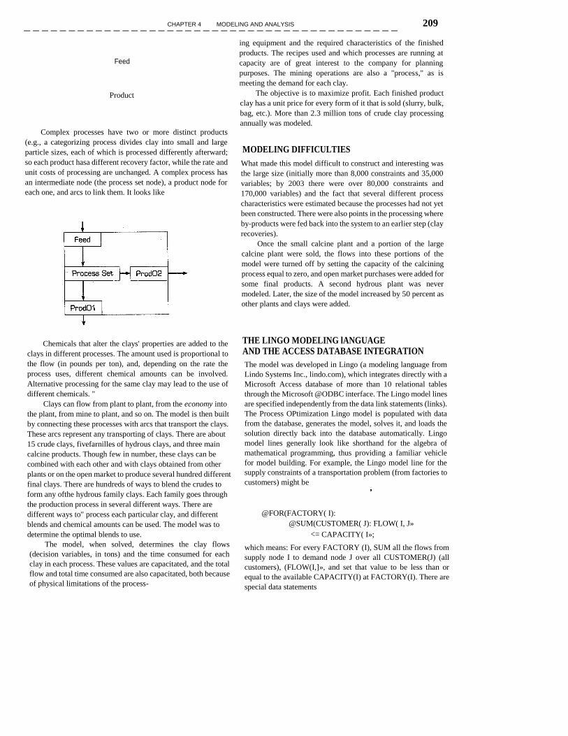
CHAPTER 4 MODELING AND ANALYSIS 209 ------------------------------------------

Feed

Product

Complex processes have two or more distinct products

(e.g., a categorizing process divides clay into small and large

particle sizes, each of which is processed differently afterward;

so each product hasa different recovery factor, while the rate and

unit costs of processing are unchanged. A complex process has

an intermediate node (the process set node), a product node for

each one, and arcs to link them. It looks like

Chemicals that alter the clays' properties are added to the

clays in different processes. The amount used is proportional to

the flow (in pounds per ton), and, depending on the rate the

process uses, different chemical amounts can be involved.

Alternative processing for the same clay may lead to the use of

different chemicals. "

Clays can flow from plant to plant, from the economy into

the plant, from mine to plant, and so on. The model is then built

by connecting these processes with arcs that transport the clays.

These arcs represent any transporting of clays. There are about

15 crude clays, fivefarnilles of hydrous clays, and three main

calcine products. Though few in number, these clays can be

combined with each other and with clays obtained from other

plants or on the open market to produce several hundred different

final clays. There are hundreds of ways to blend the crudes to

form any ofthe hydrous family clays. Each family goes through

the production process in several different ways. There are

different ways to" process each particular clay, and different

blends and chemical amounts can be used. The model was to

determine the optimal blends to use.

The model, when solved, determines the clay flows

(decision variables, in tons) and the time consumed for each

clay in each process. These values are capacitated, and the total

flow and total time consumed are also capacitated, both because

of physical limitations of the process-

ing equipment and the required characteristics of the finished

products. The recipes used and which processes are running at

capacity are of great interest to the company for planning

purposes. The mining operations are also a "process," as is

meeting the demand for each clay.

The objective is to maximize profit. Each finished product

clay has a unit price for every form of it that is sold (slurry, bulk,

bag, etc.). More than 2.3 million tons of crude clay processing

annually was modeled.

MODELING DIFFICULTIES

What made this model difficult to construct and interesting was

the large size (initially more than 8,000 constraints and 35,000

variables; by 2003 there were over 80,000 constraints and

170,000 variables) and the fact that several different process

characteristics were estimated because the processes had not yet

been constructed. There were also points in the processing where

by-products were fed back into the system to an earlier step (clay

recoveries).

Once the small calcine plant and a portion of the large

calcine plant were sold, the flows into these portions of the

model were turned off by setting the capacity of the calcining

process equal to zero, and open market purchases were added for

some final products. A second hydrous plant was never

modeled. Later, the size of the model increased by 50 percent as

other plants and clays were added.

THE LINGO MODELING lANGUAGE AND THE ACCESS DATABASE INTEGRATION

The model was developed in Lingo (a modeling language from

Lindo Systems Inc., lindo.com), which integrates directly with a

Microsoft Access database of more than 10 relational tables

through the Microsoft @ODBC interface. The Lingo model lines

are specified independently from the data link statements (links).

The Process OPtimization Lingo model is populated with data

from the database, generates the model, solves it, and loads the

solution directly back into the database automatically. Lingo

model lines generally look like shorthand for the algebra of

mathematical programming, thus providing a familiar vehicle

for model building. For example, the Lingo model line for the

supply constraints of a transportation problem (from factories to

customers) might be ,

@FOR(FACTORY( I):

@SUM(CUSTOMER( J): FLOW( I, J»

<= CAPACITY( I»;

which means: For every FACTORY (I), SUM all the flows from

supply node I to demand node J over all CUSTOMER(J) (all

customers), (FLOW(I,]», and set that value to be less than or

equal to the available CAPACITY(I) at FACTORY(I). There are

special data statements

:no PART II DECISION SUPPORT SYSTEMS

specifying all necessary data to identify the sets FACTORY,

CUSTOMER, and CAPACITY. The POP model's mining

portion looks very much like a modified transportation

problem. Limits on blends can be specified (e.g., clay B must

constitute between 80 and 95 percent of the blend).

POP DSSUSE

The DSS, written as a menu-oriented Access database table,

manages the data in the system. A particular scenario is set

up in the Access tables. through a friendly graphical user

interface (GUI) screen. The user sets the demands, makes

other adjustments to the processes, and then activates Lingo

with the click of a button. Lingo automatically generates the

entire model from its compact representation and the data as

specified in the database, and solves it. Lingo loads its

solution back into the database and returns control to the

menu-oriented GUI. Access programs then produce

managerially meaningful graphs of utilization and reports on

clay extraction and processing. Trouble spots are identified,

the case can be saved, and another scenario can be run.

For a fixed time period (one year, one quarter, two

weeks, etc.), the solution to the model indicates which mines

are active, how much clay is mined from each mine, to which

processing unit the clay is shipped from the mines, and the

appropriate crude blends (recipes) to be used. It determines

all the clay flows throughout the entire system and which

clays to purchase from the market. The model quickly

identifies which processes are running at capacity and

indicates the potential increase in profit that could be

obtained if these capacities could be increased (through

sensitivity analysis). Sometimes there 'are underutilized

processes that could handle some of the load of the limited

processes but are somewhat inefficient at doing so. Plant

managers are reluctant to use these processes but carefully

examine them and sometimes activate them.

The model also indicates how to handle the situation

now that some of the higher-quality clay mines are depleted

and new processes have been introduced. Finally,

underutilization of some processes indicates that some final

products, normally produced at other plants (not yet in the

model), could be produced at the plants represented by the

model. Several of these clays have already been added to

POP.

CASE QUESTIONS

1. What is the POP DSS used for? 2. What are the benefits of using a network-based model? 3. What are the benefits of the POP DSS?

4. How can what-if cases (scenarios) be used to determine

whether to add extra processing equipment instead of

adjusting existing processes and chemical use? 5. Could other firms that process materials use a system

like this? Why or why not?

The most interesting aspect of the model is that the

engineers and managers who structure the plants were doing

an excellent job of keeping them fine-tuned without access to

these analytical tools. The model did recommend using

different mines from time to time, and it has provided

guidance on how to manage the mines for ten years. The total

amount of clay being processed is about the same as what the

model solution recommends, which certainly helped to

validate the model. What the model is best used for is

determining how to handle the resources that are 100 percent

utilized (bottlenecks) and how to handle new and unexpected

situations, such as new clays, new demands, and new

processes. It also provides answers quickly and easily, thus

guiding managers and engineers in their decision-making.

When a plant was closed in 2001, the production and demand

for its products were moved to the main hydrous plant that

was already in the POP DSS. POP accurately determined the

blends that indicated how to handle this record throughput

optimally. Even the plant manager, initially skeptical, agreed

that his plant could handle the load once he saw POP's

recommendations.

As mentioned in Case Application 2.2, the cost of

operating a new process was determined, thus guiding

budgeting decisions for the next fiscal year. The model is

used for annual planning. It is also used in the short term for

scheduling specific large orders in with the forecasted

demands. Essentially, the POP DSS is used for strategic

planning (1-5 years), tactical planning (3-6 months), and

operational planning (2 weeks). A simple factor is changed to

generate a model that spans any needed time frame.

SUMMARY AND CONCLUSIONS

The POP model as part of the POP DSS at IMERYS is

helping to guide planning on an annual, quarterly, and even

weekly basis. It helps decision-makers determine which

options are most viable in terms of meeting clay demand at a

maximum profit. Planning for millions of tons of clay

processing is not a trivial task, and the POP DSS handles it

readily and quickly, POP continues to expand to include other

IMERYS plants and mines. The POP DSS is a success.

6. How could a demand forecasting model be integrated

with POP? (A question to think about-not in this case

application.)

7. How could the results ofthe POP DSS guide an

enterprise resource planning (ERP) system? (A question

to think about-not described in this case application. )

CHAPTER 4 MODELING AND ANALYSIS

Documents

Transcript of CHAPTER 4 MODELING AND ANALYSIS