
chapter 4 hydrogen fuelled aero engines - Cranfield University
265
CRANFIELD UNIVERSITY A J B JACKSON OPTIMISATION OF AERO AND INDUSTRIAL GAS TURBINE DESIGN FOR THE ENVIRONMENT SCHOOL OF ENGINEERING PhD THESIS
Transcript of chapter 4 hydrogen fuelled aero engines - Cranfield University

CRANFIELD UNIVERSITY
A J B JACKSON
OPTIMISATION OF AERO AND INDUSTRIAL GAS TURBINE DESIGN FOR THE ENVIRONMENT
SCHOOL OF ENGINEERING
PhD THESIS

CRANFIELD UNIVERSITY
SCHOOL OF ENGINEERING
PhD THESIS
2009
A J B JACKSON
OPTIMISATION OF AERO AND INDUSTRIAL GAS TURBINE DESIGN FOR THE ENVIRONMENT
Supervisor: P Pilidis
February 2009
This thesis is submitted in fulfilment of the requirements for the degree of Doctor of Philosophy
© Cranfield University 2009. All rights reserved. No part of this publication may be reproduced without the written permission of the copyright owner

i
DEDICATION
To my wife, Sheila To our son Hugh, our daughter Clare and her husband Michael To the memory of my devoted mother, Mary To the memory of my father, John Eric - a wonderful and inspiring man
****************

ii
ABSTRACT The aspects of gas turbine design that are explored herein are focussed on reduction or elimination of carbon dioxide (CO2) emissions and reduction of noise. There are 3 separate but related investigations. 1. Aero gas turbine engine thermodynamic cycles for subsonic transport aircraft are explored to optimise performance (thus reducing CO2 emissions) and to minimise noise; particular attention is paid to choices of fan pressure ratio, bypass ratio, installation configuration and fan design. Turbofans with long and short cowls are explored, as are propfans of various bypass ratios. The performance and noise comparisons of the engines are made using consistent technology standards; this approach is not apparently available in the literature. It is shown that relative to present day engines, useful improvements in Direct Operating Cost (DOC), fuel burn and noise are possible. It is shown, not surprisingly, that the optimum installed engine cycles for performance and noise are different. 2. The performance effects of using hydrogen fuel in “conventional” aero gas turbine engines are discussed. Also, some novel un-conventional hydrogen fuelled aero gas turbine cycles are examined. Hydrogen fuelled engines create no emissions of CO2; however, this environmental benefit is partly offset by the increased water in the engine contrails. It is shown that “conventional” engines benefit from using hydrogen fuel, measured by the thrust obtained for a given fuel energy input rate. The novel un-conventional configurations that are examined offer useful performance benefits, including significant power increases, by suitable use of the cold “sink” and high pressure of the liquid hydrogen fuel. 3. Two ways of eliminating CO2 emissions from industrial gas turbines are examined. The first is by use of hydrogen-rich fuel. There are performance gains, as with the aero engines; however in the industrial cases, the hydrogen is sometimes produced in such a way that it is mixed with substantial amounts of nitrogen, which significantly influences the results. The second is the use of CO2 in the working fluid for partially-closed and closed cycle arrangements. This permits easy sequestration of excess CO2 without the use of the large separating equipment that is necessary for extracting CO2 from the exhausts of standard open cycle plants breathing air. The changes required to a standard gas turbine to allow it to use CO2 as its working fluid are explored in some detail; this is not clearly addressed in the literature. It is shown that the turbines - the most expensive part of the gas turbine - can be operated satisfactorily but changes are sometimes required to the compressors.
******************
This thesis is offered under the Cranfield University Staff PhD scheme, Regulation 39. Hence, part of the thesis consists of relevant published papers by the author. Four such papers are included as Attachments.
***************************

iii
ACKNOWLEDGEMENTS
I acknowledge gratefully the assistance received from the following:-
Cranfield University for agreeing to let me undertake a staff PhD at age 72
My supervisor, Professor Pericles Pilidis, who encouraged and helped me whenever required, and who was a source of inspiration
Members of Cranfield University who helped in so many ways; Ken Ramsden for advice; Sarah Sheen and Gill Hargreaves for administrative support; Pablo Bellocq for invaluable assistance with preparation of charts; George Doulgeris for the noise code and assistance with its use; Andy Foster for the code giving Direct Operating Cost and Panos Laskaridis for data on engine off-takes
From outside Cranfield University: - Chris Freeman, Norman Hatton, Andrew Kempton and Jim McGuirk for technical advice; Eric Goodger for data on fuels; Mike Haines for data on hydrogen; Tom Hynes for information on distributed propulsion and Peter F. Smith for data on climate change
Most of all, I acknowledge the help of my wife, Sheila. She patiently put up with the many months that I spent immersed in papers, libraries and computers. Her wonderful support is acknowledged with gratitude and love.
************************
Better late than never The author is on the part-time teaching staff of Cranfield University. He first joined the University as a Visiting Fellow in 1997.
A. J. B. Jackson February 2009
*****************

iv
INDEX, TABLES, FIGURES
INDEX PAGE
TITLE PAGES
DEDICATIONS i
ABSTRACT ii
ACKNOWLEDGEMENTS iii
INDEX; TABLES; FIGURES iv
NOMENCLATURE viii
CHAPTER 1 INTRODUCTION AND SCOPE 1
1.1 INTRODUCTION 1
1.2 SCOPE 2
CHAPTER 2 BACKGROUND 4
2.1 BACKGROUND TECHNOLOGY 4
2.2 CLIMATE CHANGE AND CARBON DIOXIDE 6
2.3 AVIATION AND GLOBAL WARMING 8
2.4 NOISE 9
CHAPTER 3 AERO ENGINE OPTIMISATION 13
3.0 INTRODUCTION AND SCOPE 14
3.1 PERFORMANCE OPTIMISATION 18
3.2 NOISE OPTIMISATION 69
3.3 FAN DESIGN 92
3.4 ENGINE WEIGHT 97
3.5 DIRECT OPERATING COST AND FUEL BURN 109
3.6 OPEN ROTORS AND PROPFANS 116
3.7 CONCLUSIONS – AERO ENGINE OPTIMISATION 136
CHAPTER 4 HYDROGEN FUELLED AERO ENGINES 139
4.0 HYDROGEN FUELLED AERO ENGINES - BACKGROUND 140
4.1 HYDROGEN AS AN AERO ENGINE FUEL 144
4.2 CONVENTIONAL AERO ENGINES USING HYDROGEN FUEL 150
4.3 NOVEL AERO ENGINE CYCLES USING HYDROGEN FUEL 154
4.4 NOISE EFFECTS OF HYDROGEN FUEL 163
4.5 CONCLUSIONS – HYDROGEN FUELLED AERO ENGINES 163
CHAPTER 5 INDUSTRIAL NOVEL CYCLES 165
5.0 INDUSTRIAL NOVEL CYCLES; PREAMBLE 166
5.1 INDUSTRIAL GAS TURBINE BACKGROUND 168
5.2 SCOPE AND OBJECTIVES 171
5.3 METHODS 172
5.4 HYDROGEN RICH FUELS IN INDUSTRIAL GAS TURBINES 185
5.5 GAS TURBINES IN CLOSED OR PARTIALLY CLOSED LOOPS 189
5.6 CONCLUSIONS – INDUSTRIAL NOVEL CYCLES 198
CHAPTER 6 OVERALL CONCLUSIONS AND FUTURE WORK 201
CHAPTER 7 REFERENCES 207
CHAPTER 8 APPENDICES 218
1 TRENT 800 MODEL - DIMENSIONS 219
2 STATION NUMBERING DIAGRAM 220
3 TRENT 892 ENGINE PERFORMANCE MODEL 221
4 VARIATION OF OPTIMUM FAN PRESSURE RATIO WITH FORWARD SPEED 224
5 TRENT 892 MODEL DATUM PERFORMANCE POINT AT CRUISE FOR STUDIES 225
6 AIR AND POWER OFFTAKES 226
7 INSTALLATION DESIGN AND PERFORMANCE AT CRUISE 228
8 INSTALLATION DIMENSIONS SUMMARY 238
9 SUMMARY OF LONG AND SHORT COWL INSTALLED CRUISE PERFORMANCE 239
10 PERFORMANCE EXCHANGE RATES AT CRUISE 244
11 V2527-A5 ENGINE PERFORMANCE MODEL 245
12 PERFORMANCE EFFECTS OF GAS PROPERTY CHANGES 246

v
CHAPTER 9 ATTACHMENTS 257
1. A. J. B. Jackson "Some Future Trends in Aero Engine Design for Subsonic Transport Aircraft".
ASME 75-GT-2.Transactions of the ASME. Journal of Engineering for Power. April 1976.
2. Stefano Boggia, Anthony Jackson and Riti Singh "Unconventional Cycles for Aero Gas Turbine
Engines Burning Hydrogen" ISABE -2001-1245; presented at the ISABE Conference in
Bangalore, 2001
3. Stefano Boggia, Anthony Jackson "Some Unconventional Aero Gas Turbines Using
Hydrogen Fuel" ASME GT-2002-30412; presented at ASME TURBO EXPO 2002 June 3-6,
Amsterdam, The Netherlands
4. A. J. B. Jackson, H. Audus and R Singh "Gas Turbine Engine Configurations for Power
Generation Cycles Having CO2 Sequestration" Paper A05903 in the Proceedings of the
Institution of Mechanical Engineers, Volume 218 Part A: Power and Energy; 2004.
TABLES
3.1.1 T892M PERFORMANCE MODEL - RR TRENT 892 RATINGS 22
3.1.2 THRUST AUGMENTATION FACTOR OF TURBOFAN RELATIVE TO ITS CORE ALONE 26
3.1.3 T892M CORE PERFORMANCE SUMMARY 27
3.1.4 COMPARISON OF VB/VC, ETA trans AND ETAfan x ETAlpt (OPTIMUM FOPR) 28
3.1.5 EFFECT OF FORWARD SPEED ON OPTIMUM FAN PRESSURE RATIO 31
3.1.6 EFFECT OF INLET TEMPERATURE ON OPTIMUM FOPR ; FIXED N-D CONDITIONS 33
3.1.7 CORE PARAMETERS USED FOR BYPASS RATIO STUDY 36
3.1.8 NUMBERS OF LP TURBINE STAGES 44
3.1.9 CHANGES IN SFC DUE TO INSTALLATION LOSSES - LONG COWLS 54
3.1.10 SFC CHANGES DUE TO INSTALLATION LOSSES; SHORT V LONG COWLS 57
3.1.11 PERFORMANCE EXCHANGE RATES 59
3.1.12 LONG COWL AND AFTERBODY DRAGS 0.2 MACH SL ISA 62
3.1.13 TAKE-OFF AND CRUISE INSTALLED PERFORMANCE 62
3.1.14 FAN WORKING LINE SHIFT CRUISE TO TAKE-OFF 64
3.2.1 ENGINES SELECTED FOR NOISE ASSESSMENT 70
3.2.2 PERFORMANCE AT 0.2 MACH SL ISA 71
3.2.3 PERFORMANCE AT 0.2 MACH SL ISA, ALL ENGINES SCALED 84
3.2.4 NUMBERS OF FAN ROTOR AND STATOR BLADES ASSUMED 85
3.2.5 DESIGN TIP SPEED EFFECT ON FAN FORWARD ARC NOISE 88
3.3.1 2 -V- 3 STREAM JET NOISE 94
3.3.2 COMPARISON OF FAN DESIGNS 95
3.4.1 WEIGHT ESTIMATION BREAKDOWN FOR TRENT 892 103
3.4.2 WEIGHT ESTIMATION BREAKDOWN FOR IAE V2527-A5 104
3.4.3 ASSUMPTIONS AND WEIGHT RATIOS OF OPEN ROTORS (PROPFANS) 107
3.4.4 ESTIMATED WEIGHTS FOR VARYING BYPASS RATIO ENGINES 108
3.5.1 FUEL BURN ASSESSMENT OF STUDY ENGINES 113
3.5.2 DOC FRACTIONS FOR B777 5000nm FLIGHT 301 PAX 115
3.6.1 PROPFAN PERFORMANCE 0.83 MACH 10670m ISA, COT 1550K 125
3.6.2 PROPFAN INSTALLED D.PT. PERFORMANCE AT 0.83 MACH 10670M, ISA 128
3.6.3 PROPFAN PERFORMANCE 0.2 MACH SL ISA 131
4.1.1 PROPERTIES OF HYDROGEN, KEROSENE, NATURAL GAS AND AIR 146
4.2.1 COMPARISON OF PERFORMANCE FOR HYDROGEN AND KEROSENE FUELS 151
4.2.2 COMPARISON OF FUELS IN V2527-A5 ENGINE 153
4.3.1 COMPARISON OF NOVEL CYCLE PERFORMANCE 162
5.3.1 MODERN REFERENCE ENGINE COMPARED WITH 3 LARGE INDUSTRIAL ENGINES 173
5.3.2 THERMODYNAMIC PROPERTIES OF VARIOUS GASES 175
5.4.1 OPTION 1A AND 1B PERFORMANCE - SLS, ISA 187
5.5.1 OPTION 2 - PERFORMANCE; MODERN REFERENCE ENGINE - SINGLE SHAFT 191
5.5.2 OPTION 3 - PERFORMANCE; MODERN REFERENCE ENGINE - SINGLE SHAFT 194
5.6.1 COMPARISON OF NOVEL CYCLES - CONNECTED SHAFT RESULTS 199
A3.1 TRENT 892 PERFORMANCE MODEL (T892M) 221
A6.1 AIR AND POWER OFFTAKES 227
A8.1 INSTALLATION DIMENSIONS 238
A11.1 V2527-A5 PERFORMANCE MODEL 245
A12.1 GAS PROPERTIES (ROUNDED) 246
A12.2 COMPRESSOR OPERATION 248
A12.3 TURBINE OPERATION 251
A12.4 ENGINE OPERATION 255
vi
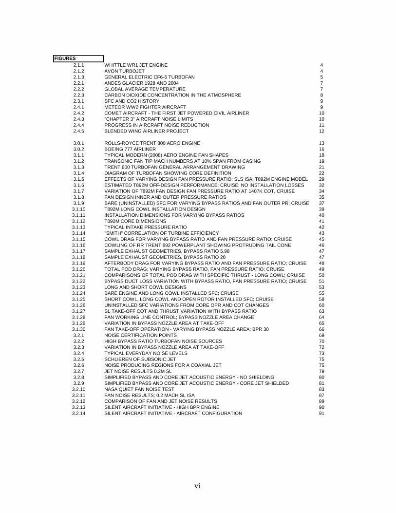
FIGURES
2.1.1 WHITTLE WR1 JET ENGINE 4
2.1.2 AVON TURBOJET 4
2.1.3 GENERAL ELECTRIC CF6-6 TURBOFAN 5
2.2.1 ANDES GLACIER 1928 AND 2004 7
2.2.2 GLOBAL AVERAGE TEMPERATURE 7
2.2.3 CARBON DIOXIDE CONCENTRATION IN THE ATMOSPHERE 8
2.3.1 SFC AND CO2 HISTORY 9
2.4.1 METEOR WW2 FIGHTER AIRCRAFT 9
2.4.2 COMET AIRCRAFT - THE FIRST JET POWERED CIVIL AIRLINER 10
2.4.3 "CHAPTER 3" AIRCRAFT NOISE LIMITS 10
2.4.4 PROGRESS IN AIRCRAFT NOISE REDUCTION 11
2.4.5 BLENDED WING AIRLINER PROJECT 12
3.0.1 ROLLS-ROYCE TRENT 800 AERO ENGINE 13
3.0.2 BOEING 777 AIRLINER 16
3.1.1 TYPICAL MODERN (2008) AERO ENGINE FAN SHAPES 18
3.1.2 TRANSONIC FAN TIP MACH NUMBERS AT 10% SPAN FROM CASING 19
3.1.3 TRENT 800 TURBOFAN GENERAL ARRANGEMENT DRAWING 21
3.1.4 DIAGRAM OF TURBOFAN SHOWING CORE DEFINITION 22
3.1.5 EFFECTS OF VARYING DESIGN FAN PRESSURE RATIO; SLS ISA; T892M ENGINE MODEL 29
3.1.6 ESTIMATED T892M OFF-DESIGN PERFORMANCE; CRUISE; NO INSTALLATION LOSSES 32
3.1.7 VARIATION OF T892M FAN DESIGN FAN PRESSURE RATIO AT 1407K COT, CRUISE 34
3.1.8 FAN DESIGN INNER AND OUTER PRESSURE RATIOS 35
3.1.9 BARE (UNINSTALLED) SFC FOR VARYING BYPASS RATIOS AND FAN OUTER PR; CRUISE 37
3.1.10 T892M LONG COWL INSTALLATION DESIGN 39
3.1.11 INSTALLATION DIMENSIONS FOR VARYING BYPASS RATIOS 40
3.1.12 T892M CORE DIMENSIONS 41
3.1.13 TYPICAL INTAKE PRESSURE RATIO 42
3.1.14 "SMITH" CORRELATION OF TURBINE EFFICIENCY 43
3.1.15 COWL DRAG FOR VARYING BYPASS RATIO AND FAN PRESSURE RATIO: CRUISE 45
3.1.16 COWLING OF RR TRENT 892 POWERPLANT SHOWING PROTRUDING TAIL CONE 46
3.1.17 SAMPLE EXHAUST GEOMETRIES, BYPASS RATIO 5.98 47
3.1.18 SAMPLE EXHAUST GEOMETRIES, BYPASS RATIO 20 47
3.1.19 AFTERBODY DRAG FOR VARYING BYPASS RATIO AND FAN PRESSURE RATIO; CRUISE 48
3.1.20 TOTAL POD DRAG; VARYING BYPASS RATIO, FAN PRESSURE RATIO; CRUISE 49
3.1.21 COMPARISONS OF TOTAL POD DRAG WITH SPECIFIC THRUST - LONG COWL; CRUISE 50
3.1.22 BYPASS DUCT LOSS VARIATION WITH BYPASS RATIO, FAN PRESSURE RATIO; CRUISE 51
3.1.23 LONG AND SHORT COWL DESIGNS 53
3.1.24 BARE ENGINE AND LONG COWL INSTALLED SFC; CRUISE 55
3.1.25 SHORT COWL, LONG COWL AND OPEN ROTOR INSTALLED SFC; CRUISE 58
3.1.26 UNINSTALLED SFC VARIATIONS FROM CORE OPR AND COT CHANGES 60
3.1.27 SL TAKE-OFF COT AND THRUST VARIATION WITH BYPASS RATIO 63
3.1.28 FAN WORKING LINE CONTROL; BYPASS NOZZLE AREA CHANGE 64
3.1.29 VARIATION IN BYPASS NOZZLE AREA AT TAKE-OFF 65
3.1.30 FAN TAKE-OFF OPERATION - VARYING BYPASS NOZZLE AREA; BPR 30 66
3.2.1 NOISE CERTIFICATION POINTS 69
3.2.2 HIGH BYPASS RATIO TURBOFAN NOISE SOURCES 70
3.2.3 VARIATION IN BYPASS NOZZLE AREA AT TAKE-OFF 72
3.2.4 TYPICAL EVERYDAY NOISE LEVELS 73
3.2.5 SCHLIEREN OF SUBSONIC JET 75
3.2.6 NOISE PRODUCING REGIONS FOR A COAXIAL JET 75
3.2.7 JET NOISE RESULTS 0.2M SL 79
3.2.8 SIMPLIFIED BYPASS AND CORE JET ACOUSTIC ENERGY - NO SHIELDING 80
3.2.9 SIMPLIFIED BYPASS AND CORE JET ACOUSTIC ENERGY - CORE JET SHIELDED 81
3.2.10 NASA QUIET FAN NOISE TEST 83
3.2.11 FAN NOISE RESULTS; 0.2 MACH SL ISA 87
3.2.12 COMPARISON OF FAN AND JET NOISE RESULTS 89
3.2.13 SILENT AIRCRAFT INITIATIVE - HIGH BPR ENGINE 90
3.2.14 SILENT AIRCRAFT INITIATIVE - AIRCRAFT CONFIGURATION 91

vii
3.3.1 DIAGRAM OF EXHAUST CONFIGURATIONS 93
3.3.2 COMPRESSOR EFFICIENCY CORRELATION 96
3.4.1 NACELLE ELEMENTS FOR WEIGHT ESTIMATION 107
3.4.2 ESTIMATED BARE AND INSTALLED WEIGHTS - VARYING BPR AND INSTALLATIONS 108
3.5.1 RELATIVE FUEL BURN FOR STUDY ENGINES 114
3.5.2 RELATIVE DOC FOR STUDY ENGINES 115
3.6.1 ROLLS-ROYCE DART ENGINE MOUNTED ON FOKKER F27 116
3.6.2 VISCOUNT AIRCRAFT 117
3.6.3 STARSHIP 117
3.6.4 HAMILTON STANDARD'S PROPFAN 118
3.6.5 GE36 UDF® ON MD 80 118
3.6.6 P&W / ALLISON PROPFAN DESIGN 119
3.6.7 A400M EUROPEAN MILITARY HEAVY LIFT PROJECT 119
3.6.8 NASA SWIRL RECOVERY TEST 120
3.6.9 ROLLS-ROYCE COWLED PROPFAN CONCEPT, 1992 120
3.6.10 NK-93 RUSSIAN COWLED PROPFAN PROJECT 121
3.6.11 EASYJET PROPFAN PROJECT 121
3.6.12 PROPFAN WIND TUNNEL TEST 126
3.6.13 DESIGN INSTALLED SFC; 0.83 MACH, 10670m, ISA - T892M CORE 128
3.6.14 EFFICIENCY BENEFITS OF PROPFANS 129
3.6.15 COMPARISON OF PROPFAN AND COWLED INSTALLATIONS 130
3.6.16 PROPFAN WIND TUNNEL TEST 131
3.6.17 GULFSTREAM AIRCRAFT WITH TEST PROPFAN 132
3.6.18 GULFSTREAM AIRCRAFT NOISE TEST RESULTS 133
3.6.19 NOISE TEST RESULTS; GE UDF® PROPFAN ON MD-80 AIRCRAFT 133
3.6.20 FLIGHT NOISE TEST COMPARISONS 134
3.6.21 OPEN ROTOR NOISE AND SFC 134
3.7.1 DOC, FUEL BURN AND NOISE FOR STUDY ENGINES 137
4.0.1 IMAGE FROM EU CRYOPLANE PUBLISHED REPORT 139
4.0.2 MACH 2.7 PROJECT 140
4.0.3 MACH 5 AIRLINER PROJECT 141
4.0.4 ARIANE ROCKET LAUNCH 141
4.0.5 B-57 IN NASA TEST OF H2 FUEL 142
4.1.1 CONTRAILS OVER NORTHERN EUROPE 148
4.2.1 V2527-A5 TURBOFAN ENGINE 151
4.3.1 AUX FUEL CYCLE 156
4.3.2 TOPPING CYCLE 157
4.3.3 ENGINE "A"; PRE-COOLED 157
4.3.4 ENGINE "B"; TOPPING CYCLE 158
4.3.5 ENGINE "B" TOPPING CYCLE ROTOR AND COMBUSTOR 159
4.3.6 ENGINE "C"; COOLED COOLING AIR 160
5.0.1 ROLLS-ROYCE INDUSTRIAL TRENT ENGINE 165
5.1.1 THERMAL EFFICIENCY TREND 168
5.3.1 Cp FOR HYDROGEN COMBUSTION IN AIR 178
5.3.2 COMPRESSOR PERFORMANCE CHARACTERISTIC - SKETCH 179
5.3.3 MRE COMPRESSOR PERFORMANCE CHARACTERISTIC 182
5.3.4 TYPICAL TURBINE CHARACTERISTICS 184
5.5.1 OPTION 2 - PARTIALLY CLOSED CYCLE 190
5.5.2 OPTION 3 - CLOSED CYCLE; CO2 WORKING FLUID; NATURAL GAS FUEL 193
A1.1 ROLLS-ROYCE TRENT 800 ENGINE ARRANGEMENT 219
A2.1 STATION NUMBERING FOR 3-SHAFT TURBOFANS 220
A3.1 TRENT 892 PERFORMANCE MODEL DETAILS SLS ISA TAKE-OFF 222
A3.2 TRENT 892 OFF-DESIGN PERFORMANCE; 0.83 MACH, 10670m, ISA 223
A5.1 TRENT 892 ENGINE ESTIMATED PERFORMANCE; 1550 COT, 0.83 MACH, 10670m, ISA 225
A11.1 V2500-A5 TURBOFAN TAKE-OFF PERFORMANCE MODEL 245
A12.1 DIAGRAM OF COMPRESSOR STAGE 247
A12.2 DIAGRAM OF TURBINE STAGE 250
A12.3 ENGINE STATION DIAGRAM 254
FIGURES - CONTINUED

viii
NOMENCLATURE ACRONYMS STATION NUMBERING SYMBOLS GREEK SYMBOLS SUFFICES
ACRONYMS AE Acoustic Energy AIAA American Institute of
Aeronautics and Astronautics ARC Aero Research Council ASME American Society of
Mechanical Engineers BPR Bypass ratio Btu British Thermal Unit CAA Civil Aviation Authority CCPLOSS Combustor Pressure
Loss CCGT Combined Cycle Gas Turbine CFD Computational Fluid Dynamics Clg Cooling COT Combustor outlet temperature CHP Combined Heat and Power dB Decibels DF Diffusion Factor DNS Direct Numerical Simulation DOC Direct Operating Cost DP Design Point EASA European Aviation Safety Agency EGT Exhaust Gas Temperature EMF Exhaust Mass Flow EPA Environmental Protection
Agency EPNL Effective Perceived Noise
Level ESDU Engineering Sciences Data
Unit eta Efficiency EU European Union F Thrust
FAA Federal Aviation Authority FAR Fuel / Air ratio FB Fuel burn FIPR Fan inner pressure ratio FOPR Fan outer pressure ratio FPR Fan pressure ratio far Fuel - Air Ratio FIG Figure GasTurb Performance code GE General Electric GHG Greenhouse Gas Gt Giga Tonnes (1 Gt = 109
tonnes) GW Giga Watts (1GW = 109 Watts) H.E. Heat exchanger HP High pressure HR Heat Rate HRSG Heat Recovery Steam
Generator ICAO Convention on International
Civil Aviation IEA International Energy Agency IGCC Integrated Gasification
Combined Cycle IP Intermediate pressure IPPC Inter-governmental Panel on
Climate Change ISA International Standard
Atmosphere ISABE International Society for Air
Breathing Engines ITP Industria de Turbo Propulsores IVP Inverted Velocity Profile KE Kinetic energy kg Kilogrammes kJ Kilo Joules kN Kilo Newtons kPa Kilo Pascals kW Kilowatts LD Disc loading L/D Lift to drag ratio LES Large Eddy Simulation LHV Lower Heating Value LH2 Liquid hydrogen

ix
LP Low pressure LPT Low pressure turbine M or Mach Mach Number MRE Modern Reference Engine MTOW Maximum take-off
weight MW Megawatts or Molecular
Weight NASA National Aeronautics and
Space Administration NdN Non-Dimensional Rotational
Speed NdW Non-Dimensional Mass Flow
Rate NGTE National Gas Turbine
Establishment NGV Nozzle Guide Vane NSNG North Sea Natural Gas NTP Normal temperature and
pressure OGV Outlet Guide Vane OPR Overall Pressure Ratio Pa Pascals P&W Pratt and Whitney pax Passengers PNdB Perceived Noise Decibels Poly Polytropic ppm Parts per million PR Pressure Ratio Pr Prandtl Number R.Ae.S. Royal Aeronautical Society R&D Research and Development RANS Reynolds Averaged
Navier-Stokes RIT Rotor Inlet Temperature RPM (rpm) Revolutions per minute RR Rolls-Royce SAE Society of Automotive
Engineers SAI Silent Aircraft Initiative SBAC Society of British Aircraft
Constructors SCR Selective Catalytic Reducer
(Reduction) SEC Specific Energy Consumption
SFC Specific Fuel Consumption SHP Shaft horsepower SLS Sea level static SL Sea Level SNECMA Societe Nationale d’Etude
et de Construction de Moteurs d’Aviation
SOT Stator Outlet Temperature SRV Swirl Recovery Vane STOL Short take-off and landing TET Turbine Entry Temperature T/O Take-off TURBOMATCH Performance code T892M Engine model name UDF Unducted fan UHB Ultra high bypass ratio UHC Unburned Hydrocarbons UK United Kingdom USA United States of America VARIFLOW Performance code Vppm Volume parts per million VTAS True Air Speed VTOL Vertical Take-off and Landing WT Weight WW2 World War 2
STATION NUMBERING Please see APPENDIX 2
SYMBOLS Please note that a few other symbols, used briefly, are defined in the local text and are not included in the list below. a Sound velocity of environment A Flow Area AR Aspect Ratio c Speed of Sound CH2 Kerosene type fuels

x
CH4 Methane CO Carbon Monoxide CO2 Carbon Dioxide CP Power Coefficient Cp Specific Heat at Constant
Pressure CT Thrust Coefficient Cv Specific Heat at Constant
Volume D Diameter Fd Inlet momentum drag Fg Gross thrust Fn Net thrust g Grams H, or h Enthalpy h Heat Transfer Coefficient or
hub/tip ratio H2 Hydrogen H2O Water or steam J Joules, or Advance Ratio K Degrees Kelvin L Length l litre m metres, mass N, n Rotational speed (rpm);
number of stages; number of blades
N2 Nitrogen Nm Nautical miles NOx Nitrous Oxides Nu Nusselt Number O2 Oxygen P Total Pressure p Static Pressure Pr Prandtl Number r Radius R Gas Constant Re Reynolds Number rho Density s Seconds s/c Space to chord ratio T Total Temperature t Static Temperature Tc Total Temperature of Cooling U Blade Speed
V Velocity Va/U Flow coefficient V0 Flight speed W Mass Flow Rate Wf Fuel mass flow rate Wn Mass flow rate station “n” Z Scaling of thrust/weight ratio
GREEK SYMBOLS γ Ratio of specific heats Cp / Cv
Efficiency
poly Polytropic Efficiency
th Thermal Efficiency
trans Transfer efficiency
Density µ Bypass ratio Δ Difference ΔH/U2 Aerodynamic loading
SUFFICES a Axial; afterbody amb Ambient AU All-up B Bypass b Burner c Cooling; cowl C Core Cr Cruise E Engine f Fuel fan Fan FL Fuel FS Fuselage g Gas J or j Jet LPT LP turbine MTOW Maximum take-off
weight

xi
m Mean N Nozzle n Net opt Optimum PA Payload PP Powerplant prop Propeller s Structural T Tip; turbine TJ Turbojet T/O Take-off trans Transfer w Whirl WI Wing 0 Ambient

1
CHAPTER 1
INTRODUCTION AND SCOPE 1.1 INTRODUCTION In the 1930s, the advent of the jet engine, or gas turbine, for aircraft propulsion brought with it many well-known benefits. From humble beginnings as a novel form of propulsion system for military fighter aircraft in WW2, to its present dominant position as the prime engine type for large aircraft species, the gas turbine has been one of the most remarkable engineering developments in history. The gas turbine engine’s success is due in part to a fundamental difference from its predecessor, the piston engine, in that its working fluid moves in a steady stream rather than flowing intermittently. This brings compact sizes and high power-to-weight ratios. The gas turbine’s compactness makes it very suitable, in industrial form, for power production in confined spaces such as on oil platforms and in ships. Unfortunately, the jet engine also brought with it various environmental disadvantages - noise nuisance and various forms of environmentally damaging gaseous emissions. Furthermore, its fuel consumption was initially high in relation to piston engines. However, its ability to propel aircraft at fast flight speeds ensured its continued development. Whilst the environmental problems and the fuel consumption issues have been addressed with some success in the past few decades, there is still room for improvement. In industry, continuous improvement of the product is vital to commercial survival. This thesis attempts to point possible further ways forward to reduce noise and to reduce or eliminate emissions of carbon dioxide, the most damaging “greenhouse gas”. Reductions in fuel consumption achieved without increases in combustion chamber temperatures also reduce emissions of nitrous oxide – another important “greenhouse gas”.

2
1.2 SCOPE The background to the topic of this thesis is described in Chapter 2, which reviews briefly the key elements of global warming and the effects of atmospheric carbon dioxide (CO2). Also, a few comments are made on the current status of aero gas turbine noise. Combustion of hydrocarbon fuels creates emissions of CO2, the most damaging “greenhouse gas”; so to address the specific fuel consumption of gas turbines is important for the environment as well as being crucial to the commercial success of the air transport system. In this thesis, gas turbine emissions of smoke and unburned hydrocarbons are not addressed, as these are essentially non-existent in modern gas turbines. Nitrous oxide emissions are problematic as they increase as combustion temperatures increase; and for gas turbines, as is well-known, increased design combustion temperatures are desirable in that they improve thermal efficiency and contribute to reducing engine size and weight. The reduction of nitrous oxide emissions is largely a matter for combustion design, which is not the focus of the present document (it would, in any case, be a topic on its own for several theses). Nitrous oxides are of course automatically reduced by fuel consumption decreases achieved without changes to the combustion chamber temperatures. The first main technical element presented (Chapter 3) is the largest study in this thesis and addresses fuel consumption and noise of aero gas turbines burning standard aviation kerosene. The starting point is today’s modern practice. The effects of changing the design thermodynamic cycle on installed fuel consumption (and hence emissions of carbon dioxide) of aero turbofan engines and propfans for civil subsonic transport aircraft are explored. The work concentrates on the choice of bypass ratio (the ratio of the bypass flow to the core flow in a turbofan), the design of the fan and the installation design. Comments are also made on the effects of changing the core engine design parameters. The effects of these design changes on turbofan jet noise and fan noise are explored. Propfan noise is examined and found problematic. As far as possible, a consistent standard of technology is used over the full range of bypass ratios, including the open rotor (propfan) cycles – this approach is not apparently available in the literature. The second main technical element in this thesis (Chapter 4) is an account of the author’s work for Cranfield University on an EU research project on hydrogen-fuelled aircraft (the so-called “Cryoplane”). Hydrogen fuelled engines emit zero carbon dioxide; however they emit more water vapour than kerosene-fuelled engines, which contributes to global warming. The Cranfield University contribution was the entire propulsion package research. The author managed the package on behalf of the University and also made a technical research

3
contribution to it. “Conventional” turbofans are examined using hydrogen fuel. Some novel cycles are also explored. The third main element (Chapter 5) is an account of the author’s work for a contract placed on Cranfield University by the International Energy Agency (IEA) which was aimed at exploring various methods of designing and configuring industrial gas turbines so that they emitted no carbon dioxide to the atmosphere. Hydrogen-rich fuels were explored as were gas turbines in closed and partially closed loop configurations. The author managed this activity for the University and made a research technical contribution. A by-product of the work was a new Cranfield University performance code for industrial gas turbines (“Variflow”) capable of estimating the performance of gas turbines using any gas as working fluid and combusting any fuel. The methods used in creating this code are described. Four relevant papers written by the author (three with co-authors) are included as attachments. These are an integral part of this thesis, as is permitted for Staff PhD candidates.

4
CHAPTER 2
BACKGROUND 2.1 BACKGROUND TECHNOLOGY
It is well known that the jet engine was conceived as a possible means of aircraft propulsion during the 1920s and 1930s; Whittle and O’Hain proposed the jet engine concept concurrently – there is much literature available about the history in websites and in books, such as Whittle’s own book “Jet: the Story of a Pioneer” [2.1]. Jet powered fighters saw service at the end of WW2. The early Whittle engines were simple turbojets with one shaft and centrifugal compressors (FIG 2.1.1). The first O’Hain engine had an axial compressor. Combustors consisted of a number of individual chambers.
During the 1940s the jet engine was very much in its infancy, although soon after WW2 gas turbines, in the form of turboprops, powered aircraft in airline service (the first was the Vickers Viscount with Dart engines – see Section 3.6). The 1950s saw the development of the axial compressor into a viable machine, which spawned new turbo-jets and new low bypass ratio turbo-fans; they entered airline service in aircraft such as the De Havilland Comet, powered by the Rolls-Royce Avon engine (FIG 2.1.2), and the Boeing 707 powered by the P&W JT3D.
FIG 2.1.1 WHITTLE WR1 JET ENGINE (IMAGE COURTESY ROLLS-ROYCE)
FIG 2.1.2 AVON TURBOJET (IMAGE COURTESY ROLLS-ROYCE)

5
By the late 1950s, the turbo-fan had ousted the turbojet as the preferred engine for civil aircraft; however, bypass ratios remained low – in the range 0.4 (RR Conway) to 1.3 (P&W JT8D). There were many new civil aircraft at the time, including the De Havilland Trident, the Vickers VC10, the Douglas DC8 and the Boeing 727 and 737. The first high bypass ratio engine to be operational was the GE TF39 in the C5 military transport. Its bypass ratio was 8 and it was the first aero gas turbine engine with a single stage fan (there was also a “half stage” at the fan root). During the late 1960s, all the major engine companies were developing high bypass ratio engines with single stage fans. Rolls-Royce offered the bypass ratio 5 RB178 turbofan for the Boeing 747 and were later successful in having a scaled down RB178 (the RB211) selected for the Lockheed Tristar. P&W had won the B747 first place with their JT9D (bypass ratio 5). Both RR and GE (with their bypass ratio 6 CF6 – FIG 2.1.3) later won places on the B747, and GE won a place on the Douglas DC10. The Boeing 747, Tristar and DC10 were the first of the generation of large twin-aisle civil transport aircraft.
The huge change of design bypass ratio incorporated in these engines, relative to the previous generation of turbofans, caused major development problems for RR, GE and P&W. However, all the technical and financial problems were eventually solved; high bypass ratio turbofans, with single stage fans were established as the
FIG 2.1.3 GENERAL ELECTRIC CF6 - 6 TURBOFAN [2.2]

6
norm for subsonic aircraft propulsion. Relative to the low bypass ratio turbofans of the early 1960s, they offered 25% better fuel consumption and about 18dB less noise – both these resulting mainly from greatly reduced jet velocities. Reducing jet velocity directly improves propulsive efficiency; also, jet noise acoustic energy, according to Lighthill’s analogy, is proportional to the jet velocity to the 7th power [2.3], so small jet velocity reductions have a large impact on jet noise. The Concorde aircraft, designed for cruising flight at Mach 2 was also in development at this time. The engine requirements for Mach 2 are very different from those for cruising at Mach 0.8 – slimness for low drag is important. Furthermore, good propulsive efficiency is obtained with high jet velocities at Mach 2, although this leads to a massive jet noise problem at take-off. Since then, turbofan bypass ratios for cruising at Mach 0.8 have risen slowly as a natural consequence of technology advances in pursuit of better fuel consumption and also continued pressure from the noise lobby. The latest favoured bypass ratios are around 6 to 9. All the major engine companies are continually improving their products, and this involves selection of the best bypass ratio to meet requirements. The author contributed to such work in the 1960s and early 1970s and published in 1975 a summary of this work [2.4] (attached). The choice of bypass ratio in the modern environment is a major study in this thesis, which therefore updates the author’s 1975 studies. It is important to update cycle optimisation studies from time to time because optimum bypass ratio and fan pressure ratio are functions of the technology standard of the core engine. Gas turbine technology is continuously being improved by research to produce engines that are better in all respects. Since the late 1950s, overall pressure ratios have risen from about 15 to over 40 and take-off turbine entry temperatures have risen from about 1400K to over 1800K. The benefits of high turbine entry temperatures and overall pressure ratios on engine performance are well known and are documented in various textbooks such as Cohen et al [2.5] and Walsh et al [2.6]. Component efficiencies and blade cooling systems have also shown remarkable improvements.
2.2 CLIMATE CHANGE AND CARBON DIOXIDE Since the early days of high bypass ratio turbofans - the 1970s - climate change has become of significant public interest and there are lobbies to reduce emissions of CO2 and other “greenhouse gases” such as NOx and H2O. A few key points about climate change and related efforts in the aviation industry are now presented, focussing on CO2, which contributes 60% of the global warming effect [2.7].

7
There is considerable controversy about whether climate change is a problem and also opinions differ as to whether the rising content of CO2 in the atmosphere and the rising atmospheric temperature are caused by man. The Meteorological Office is the “official” UK body concerned with climate change and much work is also done by the Tyndall Centre. The UK Government is party to an international
organisation, the Inter-Governmental Panel on Climate Change (IPCC) set up to pool research and to advise participating Governments. The Hadley Centre of the UK Met Office is an adviser to the IPCC.
The first key point is that there is overwhelming evidence that global warming is actually taking place. There are visible effects such as melting glaciers (FIG 2.2.1) [2.8], reduction in the size of the Arctic ice cap, increased frequency of flooding in the Severn Valley and rising sea level (very noticeable in Venice). These effects are supported by accurate measurements of global temperatures taken by the Met Office since 1850 (FIG 2.2.2) [2.9]. Global temperatures have risen by about 0.8C since 1910 and have increased by about 0.3C over the past 20 years.
The second key point is that the CO2 content of the atmosphere is already somewhat higher than at any time in the past 400,000 years according to some measurements taken from the air trapped in bubbles in the Vostok ice (FIG 2.2.3); the highest concentration until recent times is about
FIG 2.2.1 ANDES GLACIER 1928 AND 2004 (SMITH, 2008) [2.8]
FIG 2.2.2 GLOBAL AVERAGE TEMPERATURE (MET OFFICE, 2008) [2.9]

8
280ppm. However, the atmospheric CO2 content has been rising at 11Gt per annum (0.5% per annum) for the past 40 years and the present concentration is about 385ppm [2.9]. The chances of there being a correlation between temperature rise and CO2 content must be very high. The correlation with the quantities of fossil fuel used by man during the past 70 years or so also looks likely.
An IPCC Working Group published a “Summary for Policymakers” document in 2007 [2.10] which essentially supports the view that current global warming is related to the activities of mankind.
2.3 AVIATION AND GLOBAL WARMING Controversy exists about the contribution of aviation to CO2 emissions and to global warming. Aviation uses about 5-7% of the world’s oil production, which is about 2- 4% of the world’s energy output. CO2 is not the only emission from gas turbines to cause global warming – NOx and H2O together nearly double the effect of the CO2. The estimates of the total contribution of aviation to global warming vary from 2% to 13% [2.7] - a range which clearly shows the presence of vested interests. The view of the IPCC is that the figure is 3.5% [2.10]. A BBC Science and Nature programme in August 2007 [2.11] suggested that aviation might cause 3% of the EU’s total greenhouse gas emissions, but also about 7% of the UK carbon emissions. Although all these figures are small in relation to power generation, heating and motor vehicles, they are tending to grow faster than the other sources of greenhouse gas. Whatever the figures are, it is in the interests of the gas turbine industry to reduce all emissions as much as possible, in spite of the enormous improvements already made in gas turbines since the start of the jet engine era. What is being done about the environment in the aviation industry as a whole? The aircraft designers have not been idle and aircraft efficiency has improved greatly since the 1950s. A major initiative was launched in 1999 called “Air Travel
FIG 2.2.3 CARBON DIOXIDE CONCENTRATION IN THE ATMOSPHERE [2.9]

9
– Greener by Design”. This was initiated by the Royal Aeronautical Society and the SBAC and was quickly supported by all the major UK aviation organisations and industries. It has published various documents, two of which are of relevance to the gas turbine. A technical review “Greener by Design – the Technology Challenge” was published by J. E. Green in 2003 [2.12] and “Air Travel - Greener by Design” was published soon after by Lowe in 2003 [2.13]. The documents review ways forward for propulsion including higher bypass ratios, propfans, “more electric” engines and noise abatement techniques. Another event of interest to gas turbine engineering was a Conference run by the Institution of Mechanical Engineers on 20th November 2007 entitled “Novel Propulsion Systems for the 21st Century” [2.14]. Ideas such as recuperation, intercooling, propfans and pulsejets were reviewed once more and may become viable if the appropriate technology arrives. The very large improvements in engine SFC (and therefore CO2 emissions) achieved over the past half century are shown in FIG 2.3.1 [2.13].
2.4 NOISE
In the early days of the aero gas turbine engine, the jet noise problem was quickly recognised by Morley (in 1939) [2.15] and by others. Analytical and experimental work on understanding and reducing jet noise has continued ever since. The first jet propelled military aircraft were the Meteor (in the UK) with two very noisy RR Welland jet engines (FIG 2.4.1) and the German Me 262.
FIG 2.3.1 SFC AND CO2 HISTORY [2.13] (SOURCE LUFTHANSA)
FIG 2.4.1 METEOR WW2 FIGHTER AIRCRAFT [2.16]

10
After WW2, military aviation priorities for the gas turbine gave way to civil transport requirements. The main form of gas turbine for civil transport in the late 1940s and the 1950s was the turbo-prop (see Section 3.6 for more background). This form of gas turbine does not have a jet noise problem but it does have a propeller noise problem. There were far fewer civil aircraft in those days than today and the public was used to the propeller, so the noise problem subsided for a while. However, in the 1950s the demand for faster travel speeds meant that the propeller had to yield first place to jet propulsion. The Comet (FIG 2.4.2) and Boeing 707 were born, propelled by pure jets (the Avon in the Comet) or by very low bypass ratio turbofans (the JT3D in the Boeing 707). The jet noise and the compressor noise from these aircraft and others of similar technology that followed started to attract considerable adverse public comment. The noise lobby against jet aircraft was very strong in the 1960s, which was an era of considerable growth in air travel.
As a result of public pressure, aircraft now have to meet regulations regarding noise near to airports. These regulations are produced by many international and local organisations. Aircraft are categorised by the Convention on International Civil Aviation (ICAO) according to the type of aircraft and their initial in-service date (i.e. by the noise they make). Most current transport aircraft are in the “Chapter 3” category (the limits are shown on FIG 2.4.3). The noise limits that have to be met at the three flight conditions are internationally agreed and are enforced by national Certification authorities – CAA in the UK and FAA in the USA, for example.
FIG 2.4.2 COMET AIRCRAFT – THE FIRST JET POWERED CIVIL AIRLINER (NORTH EAST AIRCRAFT MUSEUM, 2008) [2.17]
FIG 2.4.3 “CHAPTER 3” AIRCRAFT NOISE LIMITS (SALFORD 2008) [2.18]

11
EASA, the European Aviation Safety Agency, works with EU national authorities on aircraft certification. In 2006, these limits were tightened by about 10dB, summed over the three conditions, and are known as “Chapter 4”. Civil transport aircraft certificated since 2006 have to meet these new limits. The advent of the “high bypass ratio turbofans” such as the P&W JT9, the Rolls-Royce RB211 and the GE CF6 in the early 1970s brought huge reductions in turbofan noise, of the order 18dB. This advance came from three changes. Jet noise fell because in high bypass ratio engines, the jet velocity is about one third that of turbojets; and since jet acoustic energy is proportional to the seventh power of jet velocity [2.3], the benefit is clear. Fan design changed from multiple stages to a single stage with no inlet guide vanes; this eliminated much of the “whining” tones caused by wakes from blade rows striking the downstream blade row. Finally, sound absorbent linings were fitted to intakes and bypass ducts. The noise lobby remains strong because despite the noise reductions described above, noise near airports is still a public nuisance. Significant research continues in the industry and academia aimed mainly at jet noise and fan noise reductions, these being the main noise sources of high bypass ratio turbofans. The progress of noise reduction in aircraft with time is summarised on FIG 2.4.4 from Envia et al (NASA, 2007)[2.19].
FIG 2.4.4 PROGRESS IN AIRCRAFT NOISE REDUCTION [2.19]
12
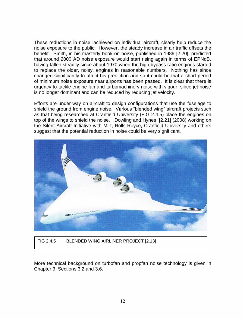
These reductions in noise, achieved on individual aircraft, clearly help reduce the noise exposure to the public. However, the steady increase in air traffic offsets the benefit. Smith, in his masterly book on noise, published in 1989 [2.20], predicted that around 2000 AD noise exposure would start rising again in terms of EPNdB, having fallen steadily since about 1970 when the high bypass ratio engines started to replace the older, noisy, engines in reasonable numbers. Nothing has since changed significantly to affect his prediction and so it could be that a short period of minimum noise exposure near airports has been passed. It is clear that there is urgency to tackle engine fan and turbomachinery noise with vigour, since jet noise is no longer dominant and can be reduced by reducing jet velocity. Efforts are under way on aircraft to design configurations that use the fuselage to shield the ground from engine noise. Various “blended wing” aircraft projects such as that being researched at Cranfield University (FIG 2.4.5) place the engines on top of the wings to shield the noise. Dowling and Hynes [2.21] (2008) working on the Silent Aircraft Initiative with MIT, Rolls-Royce, Cranfield University and others suggest that the potential reduction in noise could be very significant.
More technical background on turbofan and propfan noise technology is given in Chapter 3, Sections 3.2 and 3.6.
FIG 2.4.5 BLENDED WING AIRLINER PROJECT [2.13]

13
CHAPTER 3
AERO ENGINE OPTIMISATION
FIG 3.0.1 ROLLS-ROYCE TRENT 800 AERO ENGINE
Image courtesy Rolls-Royce [3.1]
CONTENTS 3.0 INTRODUCTION AND SCOPE 3.1 PERFORMANCE OPTIMISATION 3.2 NOISE OPTIMISATION 3.3 FAN DESIGN 3.4 ENGINE WEIGHT 3.5 DIRECT OPERATING COST AND FUEL BURN 3.6 OPEN ROTORS AND PROPFANS 3.7 CONCLUSIONS – AERO ENGINE OPTIMISATION

14
3.0 INTRODUCTION AND SCOPE 3.0.1 INTRODUCTION The aero gas turbine industry is extremely competitive – Rolls-Royce, General Electric, and Pratt and Whitney (sometimes with partners) are always vying for the large amounts of money associated with airline orders for new aircraft. So they must, if they wish to remain in business, treat the optimisation of new engine designs as a continuous and critical activity. Optimisation of performance, weight, noise, cost, emissions and maintainability are vital to commercial success. The standard of technology available at the time of a new gas turbine engine project affects the selection of the optimum values of the engine key design parameters. Technology improvements are pursued relentlessly by industry. Much research is done in-house, but industry also seeks the help and advice of academia and has for many years placed substantial research contracts in Universities and other Institutions. The rate of advancement of technology has been, and remains, vigorous ever since the aero gas turbine was invented in the late 1920s. There are many examples of the effects that new technology has had on gas turbine design. Three clear instances are as follows.
1. The change from centrifugal compressors to axial compressors in the 1950s in all but the smallest engines brought higher compressor efficiencies, higher overall pressure ratios (giving higher thermal efficiencies) and lower frontal area.
2. The advent of fan designs with supersonic relative tip Mach numbers in
the 1950s and 1960s brought higher pressure ratios per fan stage. In consequence, turbofan aero engines with single stage fans and much increased bypass ratio became practical. When they were introduced in the early 1970s, high bypass ratio turbofans brought 25% better SFC and 18dB noise reduction to subsonic transport aircraft.
3. The operating turbine entry temperatures (TETs) of gas turbines have
risen steadily with time. Take-off TETs have risen from around 1400K in the late 1950s to over 1800K in 2008 – an average of about 10K per annum. This is due to a combination of improved materials and improved cooling techniques, both achieved by intensive research in industry and academia. The results have been increased thermal efficiencies, smaller cores and lighter engine weights. This trend shows no sign of reaching a plateau at present. “TET” is used herein to represent the average gas temperature at HP turbine rotor entry. The average temperature at combustor exit is called “COT”. This latter is used herein. COTs

15
are typically 60-100K hotter than TETs due to the HP NGV cooling air re-entering the main stream through film holes and trailing edge slots. 3.0.2 SCOPE The scope of this Chapter (Chapter 3) is to explore two aspects of aero turbofan optimisation that affect the environment, namely performance and noise. Improved performance means lower fuel consumption and hence lower emissions of CO2. Lower noise is clearly important for the environment, especially near airports. In this Chapter, only standard aviation kerosene fuel is addressed – hydrogen fuelled aero engines are discussed in Chapter 4. Both performance and noise are affected by many engine design features, and if all were considered, it would consume many times the effort that could be put into a document such as this. The research reported herein is therefore restricted to matters associated with the fan including open rotors and propfans; effects of changes to bypass ratio, the fan pressure ratio, the fan design and the installation are presented. These matters influence both performance and noise. Higher bypass ratio can lead to lower fuel consumption. Reduced fan pressure ratio leads to potentially lower fan noise; it also means lower bypass nozzle jet velocity and this normally means lower jet noise. Improved fan design for cowled engines, on which much resource is expended on research annually, leads to improved efficiencies and hence to lower fuel consumption. Only separate jet exhaust systems are considered herein, although jet mixing is discussed briefly. The potential benefits from short cowls, open rotors and propfans are explored. The study is based on a single core – an approximate model of the Rolls-Royce Trent 892 turbofan engine derived from public data. However, for completeness, the main effects on performance of changes to the core thermodynamic parameters (increased COT and OPR) and to changes in component efficiencies throughout the whole engine are also presented. There is much in the literature about the effect of bypass ratio choice and fan design on both performance and on noise – references are provided later. However, the author has found nothing in the public domain that specifically relates optimisation of the two together. There is little doubt that the main turbofan manufacturers are working on the relation between performance and noise, but since this is sensitive commercial information, it is also reasonably certain that they will not expose their results in public. This Chapter therefore attempts to show a link between performance and noise optimisation – a link that is not, apparently, in the public domain. An academic study – the “Silent Aircraft Initiative” – is currently under way, which does have a performance spin-off. This work is described briefly in Section 3.6.

16
A paper written by the author for ASME in 1975 [2.4] addresses some of the effects on turbofan engine design associated with choice of bypass ratio and fan pressure ratio. It is an early study of performance, DOC and noise and is a starting point for the work reported in this Chapter, all of which is new. The paper [2.4] is included herein as Attachment 1 for convenience. The present work updates the 1975 study by using modern technology levels. Section 3.1 covers turbofan performance optimisation at subsonic cruise conditions and at take-off, concentrating on bypass ratio and fan pressure ratio. The drag of the nacelle and other “installation” issues, such as cabin air bleed and intake loss, have important effects on the choice of design bypass ratio and these are included in the work presented. Both “long” and “short” nacelles are considered. As noted above, the study presented is based on a model of the Rolls-Royce Trent 892 turbofan (see FIG 3.0.1, the frontispiece of this section), which powers the Boeing 777 civil airliner (FIG 3.0.2). The size of the study engine chosen is not particularly significant in the present studies, because most of the performance presented is Specific Fuel Consumption (SFC), which is a function only of the cycle parameters and the component efficiencies and, within reason, is not affected by engine size. However, it should be noted that if the study engines were scaled to too small a size, Reynolds numbers may fall to a point where some turbomachinery aerofoil drag coefficients might increase significantly in which case performance would deteriorate and suitable corrections would need to be made. Reynolds number effects are not relevant to the present studies because the engines are all of similar size and in any case are quite large. Where thrusts are presented, they are normalised by scaling the relevant engine to a fixed cruise thrust. This is necessary where take-off thrusts are being examined (because take-off is an off-design case in this work). This procedure is also adopted for the noise studies of Section 3.2.
Section 3.2 considers the effects of variations in bypass ratio and fan pressure ratio on jet noise and fan noise, and provides links between performance and
FIG 3.0.2 BOEING 777 AIRLINER [3.2]

17
noise. This noise work is shown at low levels of altitude and Mach number, appropriate to airport operations. Section 3.3 considers some aspects of fan design related to performance and noise. A new approach to choice of fan design parameters for turbofans is offered. Section 3.4 explores the variation in engine weight as bypass ratio changes; this affects the aircraft design and performance and hence overall Direct Operating Cost (DOC) and Fuel Burn (FB) for a payload range. Weight therefore has implications on the choice of design bypass ratio. Section 3.5 attempts to find a recommended optimum bypass ratio based on simple Direct Operating Cost and Fuel Burn calculations, with appropriate recognition of noise. Section 3.6 presents a review of open rotors and propfans. The potential performance benefits are calculated and noise is discussed. The problem of the size of the LP shaft for tractor propfans and high bypass ratio turbofans is acknowledged but not addressed. In practice, at high bypass ratios the core must be designed to accommodate a large LP shaft. This leads to consideration of “pusher” arrangements for high bypass engines, where the fan is rear mounted. Section 3.7 draws conclusions and suggests some ways forward.

18
3.1 PERFORMANCE OPTIMISATION 3.1.1 SCOPE The fuel consumption, size and weight of turbofans are all critical to the performance of the aircraft they power. The fuel used per passenger-kilometre is a powerful selling point for an airliner. Not only does it have a strong effect on operating economics but it directly affects the fuel burn and hence the emissions of CO2 per seat-km. This Section reports a detailed study of the effects of design bypass ratio, fan pressure ratio and installation configuration on the performance of turbofans for subsonic airliners. The effects on thrust and SFC of installation losses, namely cowl drag, intake loss, bypass duct loss, afterbody drag, and extraction of power and air for aircraft services are considered. Performance is estimated at cruise and take-off. In later Sections the effects on noise, Direct Operating Cost (DOC) and Fuel Burn (FB) are explored. The study is based on using a single core, modelled on the core of the Rolls-Royce Trent 892 aero engine; section 3.1.2 gives data sources. The Trent 892 engine has a bypass ratio of nearly 6 at cruise. The study also includes a brief discussion on the effects of using different cores with higher COT and OPR (section 3.1.15). Bypass ratios have increased over time from zero in the 1950s (the Avon in the Comet airliner) to about 5 in the 1970s (Rolls-Royce RB211 family, the General Electric CF6 family and the Pratt and Whitney JT9 family) to current values of around 8 to 9 (the latest Rolls-Royce Trent family and the recent Alliance GP 7200). The choice of bypass ratio and fan pressure ratio are crucial to performance. So also is the design of the fan itself - at the higher operating
powers, fans have supersonic relative Mach numbers at their tips and their efficiency has a strong effect on fuel consumption; typically 1% of fan efficiency is
worth 0.7% of engine fuel consumption (more details are given later). Modern fan profiles have very sophisticated shapes, designed using Computational Fluid Dynamics (CFD). Also, much resource is expended on testing of advanced ideas. FIG 3.1.1 shows typical modern fan shapes [3.3] and [3.4].
FIGS 3.1.1 TYPICAL MODERN (2008) AERO ENGINE
FAN SHAPES (REFS [3.3] AND [3.4] RESPECTIVELY)

19
The curved shapes of the fan leading edges give improved aerodynamic performance in several ways. The outer portion of the blade span, where the relative Mach number is highly supersonic (~ Mach 1.5) is swept back like the leading edge of wings of supersonic fighter aircraft, in order to reduce shock losses by inducing oblique rather than normal shocks. The tip chord is increased and the leading edge swept forward to improve blade performance in the casing boundary layer. At the mid span of the blades, the chord is increased to improve the diffusion factors; in the mid span region, the blade speed is lower than at the tip, but high pressure ratios are still required, so blade passage diffusion becomes high – wider chord is helpful. The detailed shaping of fan blades is not discussed in detail herein. However, it is a subject that attracts much attention; there is, for example, literature on the effects of sweep and lean on fan performance and noise. Denton et al in 2002 [3.5] conclude from a CFD study that “Overall, very little change in peak efficiency or pressure ratio is produced by blade sweep or lean. However, there are significant effects on stall margin and maintaining a high efficiency over a wide range”. Bergner et al in 2005 [3.6] conducted CFD studies and also testing at Darmstadt and came to a similar conclusion: “…forward sweep…..has a beneficial effect on performance and stall margin”. A paper by He
and Ismael in 1999 [3.7] shows a comparison of CFD and test results for the shock pattern at 90% span of a transonic fan blade; the complexity of the flow is clear (FIG 3.1.2). These and other papers comment on the significance of the over-tip leakage on the tip shock patterns.
3.1.2 PROCEDURE A performance model of the Rolls-Royce Trent 892 turbofan has been made using the GasTurb code [3.8]. This model is henceforth called the T892M in this document (“M” denotes “model”). A preliminary study of the effect on performance of varying the fan outer pressure ratio of the T892M
FIG 3.1.2 TRANSONIC FAN TIP
MACH NUMBERS AT 10%
SPAN FROM CASING [3.7]

20
at take-off has been done, as a design point exercise. The performance of the T892M at a typical cruise condition has been calculated (off-design) showing the variation of thrust and fuel consumption with COT. COT is used from this point onwards in preference to TET, which can be misunderstood. One of the T892M cruise operating points has been chosen as the base for a major design point study, in which the core is kept constant and variations in fan outer pressure ratio and bypass ratio are explored. Bypass ratios up to 30 have been examined, to overlap the range of uncowled (open rotor) engines. Next, sensible selections of the engines from the above study have been “installed”. This was a considerable exercise as it involved designing the cowl, bypass duct and afterbody of each engine. From this work, the installed performance of each engine has been calculated. The results provide the bypass ratio and fan pressure ratio to give the optimum installed performance. Both long and short cowls are studied. The installed take-off performance has then been calculated for some of the engines for which installed cruise performance has been found. This has involved re-calculating the installation losses at take-off. There are two purposes; first, to find out which engine gives the best take-off performance: second, to provide performance data, such as jet velocities and flows, for the noise assessments. The performance study is extended in Section 3.6 to cover open rotors and propfans. The jet noise and fan noise of each engine at take-off has been calculated and a plot made presenting the link between performance optimisation and noise optimisation – an objective of this thesis. The noise assessment is given in Section 3.2. In addition to these studies, a number of other relevant issues are presented. The proof that there is an optimum design fan pressure ratio for performance for each core and bypass ratio is given. The effect of forward speed on optimum fan outer pressure ratio is presented. The effects of changing the key core design parameters are also presented and the effects of varying component design efficiencies are given, to set the whole study in context. 3.1.3 TRENT 892 PERFORMANCE MODEL – CALLED T892M The basis of the work presented in Chapter 3 is the Rolls-Royce Trent 892 engine (FIG 3.1.3). This is a modern 3-shaft turbofan with separate exhausts for the bypass and core flows. It has a single stage fan of diameter 110ins (2.794m).

21
Other key dimensions are shown in APPENDIX 1. A station diagram is shown in APPENDIX 2. A performance model of the RR Trent 892 engine has been created using the GasTurb code [3.8] and as already mentioned is denoted in this document as the T892M. The public RR Trent 892 performance information used to create the T892M is from Jane’s “Aero Engines” [3.9]. In Jane’s and elsewhere, most public information for engine performance is at sea level static take-off conditions and so the model has been created at this condition. Fortunately, at static take-off conditions, the inlet airflow, bypass ratio and overall pressure ratio are provided as well as the usual take-off thrust. Component efficiencies and COT were varied over sensible ranges until the quoted thrusts and cruise fuel consumption were achieved. Results are summarised in TABLE 3.1.1 and given fully in APPENDIX 3.
In the case of the RR Trent 892 engine, cruise thrust and specific fuel consumption (SFC) are also given in Jane’s [3.9] at 0.83 Mach, 10670m altitude (ISA has, reasonably, been assumed). The model has therefore been “flown” at this condition and the fuel flow (i.e. the “throttle setting”) has been altered until the quoted thrust was obtained. At this point the SFC was compared with the value in Jane’s; agreement was excellent. This has been instrumental in checking the component efficiency values assumed. Very good agreement with all of the public information was achieved. A summary is presented below (TABLE 3.1.1) and full details are provided in APPENDIX 3. It is worth noting that the cruise thrust published in Jane’s is clearly not the maximum cruise thrust, but a “typical” cruise thrust, near the point of best SFC. It is normal practice by the engine manufacturers to publish cruise information in this form as it shows their engines’ fuel consumption – a very competitive parameter - in the best light.
FIG 3.1.3 TRENT 800 TURBOFAN GENERAL ARRANGEMENT DRAWING [3.9]

22
TABLE 3.1.1 T892M PERFORMANCE MODEL – RR TRENT 892 RATINGS
PARAMETER UNITS PUBLIC DATA [3.9]
PERFORMANCE MODEL
DIFFERENCE %
TAKE–OFF, SLS ISA Thrust kN 407.5 407.52 Negligible
Inlet airflow rate kg/s 1200 1200 0
Bypass ratio 5.8 5.8 0
Fan pressure ratio 1.81 1.81 0
Core mass flow rate kg/s 176 176.47 +0.2
Overall pressure ratio 40.8 40.8 0
T/O ASSUMED VALUES (SEE APPENDIX 3 FOR OTHER ASSUMED PARAMETERS)
Combustor outlet temperature (COT)
K - 1794.5
CRUISE, 10670m, 0.83 M, ISA Typical cruise thrust kN 60.05 60.05 0
SFC g/s.kN 15.86 15.866 Negligible
COT K - 1407
In the T892M, the efficiencies, COT values and cooling airflow rates all had to be adjusted to match the available public data (details are in APPENDIX 3); the results are good modern values although they cannot be assumed to be precisely the RR Trent 892 engine values. 3.1.4 OPTIMUM FAN OUTER PRESSURE RATIO As is well known, for each operating point of any given turbofan core there is a value of fan outer pressure ratio that gives the best performance – thrust and SFC; optimum fan pressure ratio is clearly also a function of bypass ratio. This fact is documented variously – examples are in Refs [2.5], [2.6], [3.10] and [3.11]; and by implication in [3.12]. The “core” is defined as the whole of the compression system apart from the bypass or outer section of the fan, plus the combustor and that part of the turbine system that drives all the compression except the fan outer section. The concept is best envisaged as an “aft fan” (FIG 3.1.4).
CORE
FAN
FAN TURBINE
VB
VC
FIG 3.1.4 DIAGRAM OF TURBOFAN SHOWING CORE DEFINITION

23
Any actual turbofan engine will of course not necessarily be operating at its optimum fan outer pressure ratio for the particular conditions pertaining to the core at that moment in flight. At high power settings the fan outer pressure ratio will tend to be at slightly lower than its optimum value; at low power settings the fan outer pressure ratio can be somewhat higher than the optimum value. Furthermore, as forward speed changes the optimum fan pressure ratio changes. These matters are discussed later. So the designer of the engine cycle has to choose carefully where in the flight envelope he wants the best performance, before selecting the fan outer pressure ratio. For most turbofans, this is at “cruise”; but which of the many “cruise” options should be selected? The most important altitude, forward speed and thrust level will depend on the expected average mission – this is sometimes not clearly known from the outset. Fortunately, as will be shown, provided a sensible design selection is made, the fan operates reasonably close to its optimum outer pressure ratio for much of the cruise, climb and take-off segments of flight. In the design process, the optimum fan outer pressure ratio will depend on the core performance and the bypass ratio. It is convenient to envisage the core as defined above – that is, it includes the fan inner (or “root”) section and a small part of the LP turbine to drive it. It is possible to envisage the concept of optimum fan outer pressure ratio without resorting to equations. However, some key equations are presented shortly. Qualitatively, a fixed core – fixed COT, OPR, efficiencies and flow – may be considered. This means that the energy and flow at the entrance to the fan turbine is fixed. At any fixed bypass ratio, the fan outer pressure ratio is a design choice. Assume in the first instance that a (ridiculous) fan outer pressure ratio value of 1.0 is chosen. This is tantamount to there being no fan, and the core acts like a turbojet, with high jet velocity and hence poor propulsive efficiency.
Propulsive efficiency,
0
1
2
V
Veta
J
propulsive (≈ 0.75 for T892M) {1}
Where VJ is the fully expanded jet velocity and V0 is flight speed As fan outer design pressure ratio is increased, the core jet velocity falls because more and more energy is being transferred from the core stream to the fan stream. The jet velocity from the bypass stream rises. For a while, the propulsive efficiency increases (this is, of course why the turbofan was invented). However, the pressure downstream of the fan turbine falls and eventually would fall below atmospheric pressure. This too is ridiculous as the core flow would fall to zero. So there must be an optimum choice of fan outer pressure ratio. This is confirmed by

24
the following equations, which appeared in public lectures delivered for many years by the author, the notes for which were first published in 1973 [3.10]. The equations were brought to the author’s attention by Mr. N. G. Hatton of Rolls-Royce. The net thrust, Fn, of a simple turbojet (the core of the bypass engine) is
0VVWF Jn (Ignoring differences between inlet and outlet flows) {2}
W is the airflow rate; all jet velocities are fully expanded values. The kinetic energy added to the air stream is
2
0
2
2
1VVWKE J {3}
Supposing the exhaust stream from this turbojet is used to drive a turbine that drives the bypass (outer) section of the fan. The thrust of this engine of bypass ratio µ is now:-
00 VVWVVWF BCn {4}
VC and VB are the fully expanded exhaust velocities of the core stream and bypass stream respectively The kinetic energy from the core stream is transferred to the bypass stream with transfer efficiency, ηtrans. Thus:-
transBCJ /VVWVVWVVWKE2
0
22
0
22
0
2
2
1
2
1
2
1 {5}
The optimum amount of energy will be transferred when the thrust is a maximum,
i.e. when 0Bn V/F .
B
C
B
n
V
VW
V
F {6}
Therefore, B
C
V
V for maximum thrust {7}
The basic turbojet kinetic energy available is constant, so

25
0222
1B
transB
CC
B
TJ VV
VV.W
V
KE {8}
Therefore, C
Btrans
C
B
V
V.
V
V {9}
Thus, trans
C
B
V
V for maximum thrust. {10}
Note that CTJ
Btrans
KEKE
KE from {5} {11}
Thus engines with velocity ratio having this value will have the optimum fan outer pressure ratio for the given bypass ratio and core operating point, because the bypass stream exhaust velocity is a direct function of the fan outer pressure ratio at a flight condition (apart from minor influences of the intake and bypass duct pressure losses). It is also of interest to determine by how much the turbojet thrust is augmented by the addition of the fan to make a turbofan. At the calculated optimum condition, the thrust of the turbofan is
11 0
00
VVW
VVWVVWF
C
CCn where η = ηtrans {12}
KE gain, 2
0
22
0
2
2
111
2
1VVWVVWKE JC {13}
Therefore, 12
0
22/VVV JC {14}
And so the thrust at optimum fan pressure ratio is given by
11 0
212
0
2V.V./VWF
/
Jn {15}
The thrust of the bypass engine can now be compared with that of the basic turbojet which forms the core. Note that since the fuel flow remains constant, the increase in thrust is equal to the improvement in SFC.

26
J
JJ
turbojet.n
bypass.n
V/V
.V/V.V/V./
F
F
0
0
21
22
0
1
111 {16}
Statically (V0 = 0) this becomes 21
1turbojet.n
bypass.n
F
F {17}
The thrust gained by fitting a fan to a core is significantly greater at low forward speeds than at normal cruise speeds. This effect is even more pronounced at higher bypass ratios. To illustrate this, approximate figures for two simplified engines based on the T892M core have been substituted in equation {16}. Bypass ratios shown are 6 (approximately the T892M value) and 20. The assumed transfer efficiency, ηtrans, is 0.82; this is discussed further in Section 3.1.5. The fully expanded jet velocity, VJ, of the T892M core with no fan at take-off is about 915.5m/s and at cruise is about 892m/s; (more details of the T892M core performance are given later in TABLE 3.1.3). At 0.83 Mach, 10670m, ISA the flight speed, V0, is 246m/s. The resulting increases in thrust due to fitting optimum fans at take-off and cruise are shown in TABLE 3.1.2.
TABLE 3.1.2 THRUST AUGMENTATION FACTOR OF TURBOFAN RELATIVE TO ITS CORE ALONE (EQUATION {16})
BYPASS RATIO TAKE – OFF SLS ISA CRUISE 0.83M 10.67km
6 2.433 1.521
20 4.171 1.736
As will be shown later, (Sections 3.1.11 and 3.1.19) these figures match the detailed engine performance calculations remarkably accurately. It is already clear that increasing bypass ratio gives potentially better cruise performance. The consequence of this effect is that at low bypass ratios turbofan engines are struggling to achieve sufficient take-off thrust to match their climb and cruise capabilities. The low bypass engines of the 1950s and 1960s consumed most of their blade life at take-off. As bypass ratios increased, the engines could provide relatively greater take-off thrust levels and the flight segment that consumed blade life switched to climb, where it is largely these days. Aircraft requiring very short take-off field lengths, such as front line STOL military transports, tend to take advantage of the high take-off thrusts available from very high bypass ratios, and are therefore often fitted with turboprops. A modern example is the Airbus A400M military heavy lift project. Although the maximum cruising speed of turboprops is not generally as high as that of turbofans, this is usually not critical for STOL aircraft.

27
3.1.5 T892M TRANSFER EFFICIENCY It is of interest, to determine values of the transfer efficiency, ηtrans, as defined above, for the T892M. The first step is to determine the core engine performance in order to obtain the “turbojet” exit kinetic energy. The T892M core is defined, for the purposes of this study, as the entire compression system except for the fan outer portion plus the combustor, HP turbine, IP turbine and a small part of the LP turbine required to drive the fan inner (core) section. The overall parameters of the core at take-off, SLS, ISA, and at 0.83 Mach, 10670m, ISA are summarised below (TABLE 3.1.3). The jet velocity shown is the fully expanded jet velocity as this represents the exit kinetic energy unfettered by nozzle losses. The net thrust shown does, however, assume a convergent nozzle. TABLE 3.1.3 T892M CORE PERFORMANCE SUMMARY
UNITS TAKE-OFF CRUISE
FLIGHT CONDITION SLS, ISA 0.83 M, 10670m ISA
INLET AIRFLOW RATE kg/s 176.5 67.78
OPR 40.80 39.25
COT K 1794.5 1550
JET VELOCITY (FULLY EXPANDED)
m/s 915.5 892.0
NET THRUST (CONVERGENT) kN 165.2 44.91
SFC g/s.kN 23.84 27.63
It is of interest to compare the value of the transmission efficiency of the T892M at take-off and cruise with the ratio of bypass and core jet velocities at optimum fan outer pressure ratio (FOPR). There are detailed problems with the computations, such as the huge variation in Cp in the core jet and the matter of how to provide comparative bleeds between the core and the complete engine. So the figures below are only approximate. However, they do show equation {10} is adequate as a guide to finding optimum fan outer pressure ratio. It is also of interest to note that the product of the fan outer efficiency and LP turbine isentropic efficiency is very close to VB/VC at the optimum FOPR. The relationship can be approached analytically and the equations are very messy, requiring numerical solutions. The relationship below is close to equality at low values of VB but nevertheless remains a good guide to optimum fan pressure ratio at practical values of VB/VC. Please see TABLE 3.1.4 for comparisons.
LPTfan
C
B
V
V

28
TABLE 3.1.4 COMPARISON OF VB/VC, Eta trans AND Eta fan x Eta LPT (OPTIMUM FOPR)
ENGINE CORE T892M CORE T892M
CONDITION TAKE-OFF SLS ISA CRUISE 0.83M, 10670m, ISA
COT, K 1794.5 1794.5 1550 1550
Optimum FOPR (exact) N/A 1.823 N/A 1.813
VB m/s N/A 328.2 N/A 390.5
VC m/s 915.5 399.0 892.0 497.5
VB/VC N/A 0.823 N/A 0.785
Eta trans N/A 0.822 N/A 0.823
Eta fan x Eta LPT N/A 0.816 N/A 0.807
3.1.6 FAN OUTER PRESSURE RATIO – T892M AT TAKE-OFF The RR Trent 892 engine performance model, T892M, created at static take-off conditions and described in Section 3.1.3 incorporates the fan outer pressure ratio value of 1.81 quoted in Jane’s “Aero Engines” [3.9]. It is prudent to determine how close this value is to the optimum before proceeding further with the studies. Accordingly, design points were calculated at SLS, ISA, with the T892M core fixed, varying only the fan outer pressure ratio. For this exercise, bypass duct loss is kept constant and there is of course no cowl drag at V0 = 0. There is no extraction of air or power, and no allowances were made for inlet pressure loss and afterbody drag: these latter installation effects would have only a small influence on optimum fan outer pressure ratio values at take-off, where the engine is developing its greatest thrust. In a later part of the study, full installation losses are included at take-off, 0.2 Mach SL ISA for noise calculations. The fan and LPT turbine polytropic efficiencies are kept constant to maintain a constant level of technology. This implies that as the fan outer pressure ratio is varied, the fan design is varied to maintain constant fan quality, measured by polytropic efficiency. In practice this would perhaps mean reducing the fan tip speed as fan outer pressure ratio falls and possibly reducing the number of fan blades in the rotor and outlet guide vanes. It also implies that as the fan outer pressure ratio is varied, the number of LP turbine stages is altered to maintain a constant loading (ΔH/U2), which would imply a constant LP turbine polytropic efficiency. The overall performance results are shown FIG 3.1.5.
Also shown on FIG 3.1.5 are values of the core and bypass stream velocities, together with the ratio of these velocities, VB/VC. It is clear that the fan outer pressure ratio, 1.81, given in Jane’s “Aero Engines” [3.9] occurs close to the theoretical point for optimum performance derived in Section 3.1.4. That is, it occurs near where the value of VB/VC equals the transfer efficiency, ηtrans. This result further confirms the validity of the performance model. A precise study shows that the exact optimum is at a fan outer pressure ratio of 1.823. As

29
mentioned before, this is close to the point where the value of the product of the fan outer and LP turbine isentropic efficiencies is 0.815.
1 1.2 1.4 1.6 1.8 20
200
400
600
800
1000
VE
LO
CIT
IES
fully
exp
an
de
d -
m/s Vbypass
Vcore
CORE ONLY
1 1.2 1.4 1.6 1.8 20
2
4
6
8
Vb
yp
ass/V
co
re
1 1.2 1.4 1.6 1.8 2 2.2150
200
250
300
350
400
FAN PRESSURE RATIO
Th
rust -
kN
OPTIMUM FAN PRESSURE RATIO AT T/O
ACTUAL TRENT T/O POINT
ηFAN x ηLPT = 0.815
FIG 3.1.5 EFFECTS OF VARYING DESIGN FAN PRESSURE RATIO; SEA LEVEL STATIC, ISA; T892M ENGINE MODEL

30
FIG 3.1.5 also shows how rapidly the core exhaust velocity falls as fan outer pressure ratio rises above the optimum. At a fan outer pressure ratio of nearly 2.1, the core exhaust velocity becomes negative because the core nozzle total pressure is below atmospheric static pressure! 3.1.7 GENERAL EFFECT OF FORWARD SPEED ON OPTIMUM FAN OUTER PRESSURE RATIO The main parts of the performance studies reported in this document are at the following flight conditions:-
Take-off at sea level, static; the T892M model is created at this condition. Also, thrusts are reported at this condition as a function of bypass ratio and COT for completeness.
Take-off at 0.2 Mach, sea level; this is near the end of the take-off run (“rotation”) where high bypass ratio engines are giving much less thrust than at the start of the take-off. It is also close to the condition at which noise is important. Cruise, 0.83 Mach, 10670m, ISA; this is obviously a critical condition for fuel burn, CO2 emissions and operating economics.
Therefore, before embarking on the main studies, a short design point exercise has been carried out to isolate the effect of forward speed alone on optimum fan outer pressure ratio. A simple two shaft turbofan performance model has used with a fixed core (OPR 24, COT 1700). To ensure the calculations were not masked by changes in Cp and other spurious effects, for all three forward speeds the inlet total temperature was 288.15K and the inlet total pressure was 101.325 kPa: -
SLS, ISA; 0.2 Mach, 234.602m, ISA – 0.762oC; 0.83 Mach, 3651.315m, ISA – 11.16oC
The key results are in TABLE 3.1.5 and the details are in APPENDIX 4. From TABLE 3.1.5, it can be seen that the optimum fan outer pressure ratio increases slightly with forward speed due to the change in the nozzle Mach numbers, caused by the supercharging effect of the forward speed on the nozzle total pressures. It is therefore to be expected that at cruise conditions, the optimum fan outer pressure ratio will be higher than at take-off for a given engine “non-dimensional” operating condition – say a given COT/T2. This will be explored further.

31
TABLE 3.1.5 EFFECT OF FORWARD SPEED ON OPTIMUM FAN PRESSURE RATIO
DESIGN POINTS
SLS ISA 0.2M 0.83 M
OPT FPR1.712
FPR SAME AS SLS 1.712
OPT FPR 1.7175
FPR SAME AS SLS 1.712
OPT FPR 1.785
ITEM UNITS
Altitude m 0 234.602 234.602 3651.315 3651.315
ΔTamb rel ISA
C 0 -0.762 -0.762 -11.160 -11.160
Mach 0 0.2 0.2 0.83 0.83
P2 kPa 101.325 101.325 101.325 101.325 101.325 T2 K 288.15 288.15 288.15 288.15 288.15 W2 kg/s 700 700 700 700 700
BPR 6 6 6 6 6
COT K 1700 1700 1700 1700 1700 P45 kPa 562.3 562.3 562.3 562.3 562.3 Efficiencies Datum Datum Datum Datum Datum VB/VC 0.8074 0.7930 0.8074 0.6974 0.7872
PC/pamb 1.356 1.395 1.381 2.131 1.880
PB/pamb 1.686 1.734 1.740 2.649 2.762
Net thrust kN 224.06 182.78 182.79 118.55 118.94
3.1.8 CRUISE PERFORMANCE OF THE T892M An objective of the current work is to explore different bypass ratio designs, based on a single “common” core. The question that immediately arises is the matter of what flight condition should be chosen for the engine design points. As mentioned before, it is proposed to investigate bypass ratios up to 30 with cowled configurations. It will be shown that at bypass ratios above about 15, there are large shifts in fan working line level as forward speed increases. This effect is so severe at the highest bypass ratios that engine instability would take place if no action were taken; variable bypass nozzle area is the most effective way to counteract the problem. It is therefore prudent to perform the design points at cruise, where SFC is of prime importance. Each engine will then be run in off-design mode at take-off. It will be shown that the higher bypass ratio engines provide ample take-off thrust and can therefore afford some losses associated with non-optimum duct and nozzle shapes resulting from variable bypass nozzle hardware. 3.1.8.1 T892M CRUISE OFF-DESIGN PERFORMANCE The next step is therefore to establish the T892M performance at cruise. A flight condition of 0.83 Mach, 10670m, ISA has been chosen as this is where there is a small amount of public performance information. The “bare engine” SFC and estimated COT are shown on FIG. 3.1.6.

32
From FIG 3.1.6 it can be seen that the engine model, when operating at a COT of 1407K, closely matches the public data SFC (15.86g/s.N) at the quoted net thrust, 60.05kN (14.7% of take-off thrust). This value of COT is very low compared with the estimated take-off COT of 1794.5K. Furthermore, at this flight condition, a normal value of maximum cruise thrust is about 20% of the take-off thrust, which would be about 82kN. There is little doubt therefore that the public data does not present the maximum cruise point. However, at a cruise COT of 1550K, at 0.83 Mach, 10670m ISA, where T2 is 248.94K, the engine is operating at virtually the same “non-dimensional” point as at take-off, measured by the value of COT/T2. Hence:-
CRO/T.
..
.
.
T
COT
94248
315502286
15288
51794
2
At 1550K COT, the net thrust is estimated at 75.98kN, about 18.6% of take-off thrust – only about 6-7% of cruise thrust below a reasonable maximum cruise thrust.
55 60 65 70 75 8030
35
40
45O
PR
55 60 65 70 75 801.6
1.7
1.8
FP
R
55 60 65 70 75 801300
1400
1500
1600
CO
T -
K
55 60 65 70 75 80 8515.5
16
16.5
17
SF
C -
g/s
.kN
NET THRUST - kN
Point matching public data
Point chosen for BPR study
FIG 3.1.6 ESTIMATED T892M OFF-DESIGN PERFORMANCE; 0.83 MACH, 10670m, ISA; NO INSTALLATION LOSSES.
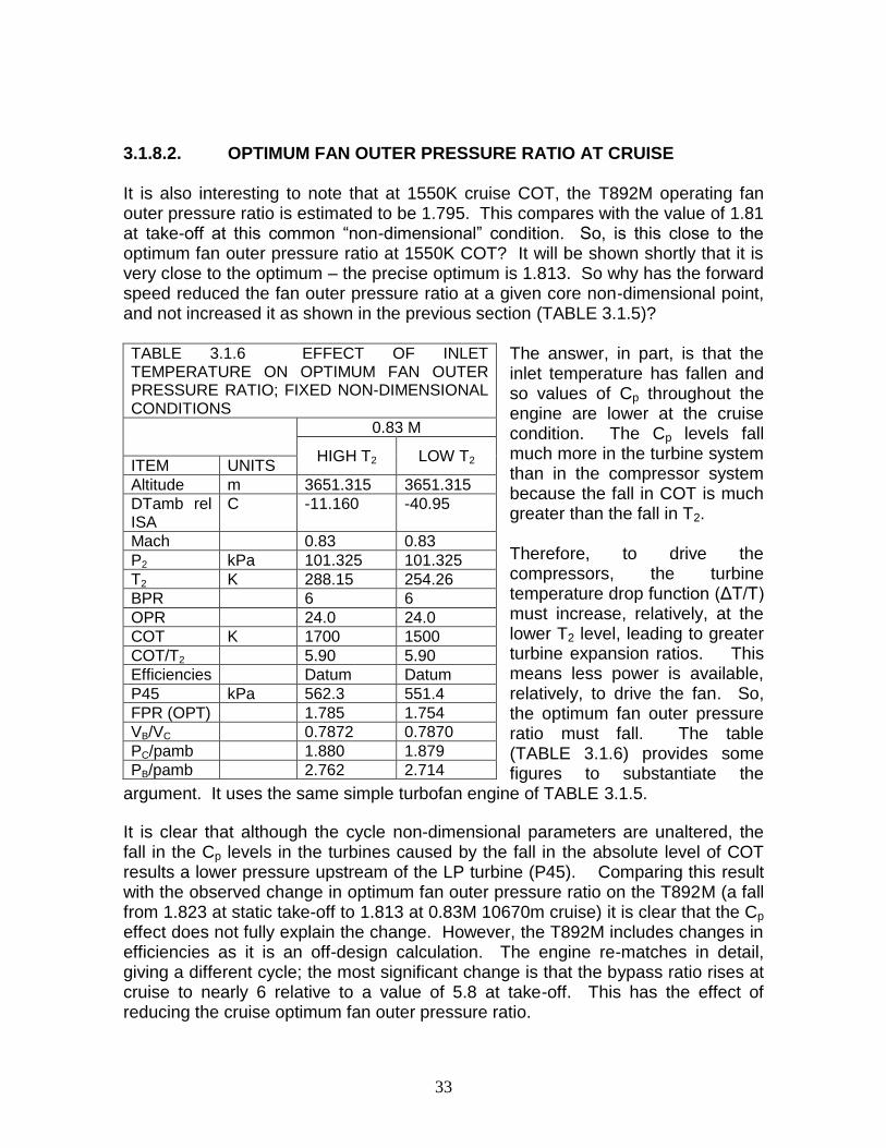
33
3.1.8.2. OPTIMUM FAN OUTER PRESSURE RATIO AT CRUISE It is also interesting to note that at 1550K cruise COT, the T892M operating fan outer pressure ratio is estimated to be 1.795. This compares with the value of 1.81 at take-off at this common “non-dimensional” condition. So, is this close to the optimum fan outer pressure ratio at 1550K COT? It will be shown shortly that it is very close to the optimum – the precise optimum is 1.813. So why has the forward speed reduced the fan outer pressure ratio at a given core non-dimensional point, and not increased it as shown in the previous section (TABLE 3.1.5)?
The answer, in part, is that the inlet temperature has fallen and so values of Cp throughout the engine are lower at the cruise condition. The Cp levels fall much more in the turbine system than in the compressor system because the fall in COT is much greater than the fall in T2. Therefore, to drive the compressors, the turbine temperature drop function (ΔT/T) must increase, relatively, at the lower T2 level, leading to greater turbine expansion ratios. This means less power is available, relatively, to drive the fan. So, the optimum fan outer pressure ratio must fall. The table (TABLE 3.1.6) provides some figures to substantiate the
argument. It uses the same simple turbofan engine of TABLE 3.1.5.
It is clear that although the cycle non-dimensional parameters are unaltered, the fall in the Cp levels in the turbines caused by the fall in the absolute level of COT results a lower pressure upstream of the LP turbine (P45). Comparing this result with the observed change in optimum fan outer pressure ratio on the T892M (a fall from 1.823 at static take-off to 1.813 at 0.83M 10670m cruise) it is clear that the Cp effect does not fully explain the change. However, the T892M includes changes in efficiencies as it is an off-design calculation. The engine re-matches in detail, giving a different cycle; the most significant change is that the bypass ratio rises at cruise to nearly 6 relative to a value of 5.8 at take-off. This has the effect of reducing the cruise optimum fan outer pressure ratio.
TABLE 3.1.6 EFFECT OF INLET TEMPERATURE ON OPTIMUM FAN OUTER PRESSURE RATIO; FIXED NON-DIMENSIONAL CONDITIONS
0.83 M
HIGH T2 LOW T2 ITEM UNITS
Altitude m 3651.315 3651.315
DTamb rel ISA
C -11.160 -40.95
Mach 0.83 0.83
P2 kPa 101.325 101.325 T2 K 288.15 254.26 BPR 6 6
OPR 24.0 24.0
COT K 1700 1500 COT/T2 5.90 5.90
Efficiencies Datum Datum P45 kPa 562.3 551.4
FPR (OPT) 1.785 1.754
VB/VC 0.7872 0.7870
PC/pamb 1.880 1.879
PB/pamb 2.762 2.714

34
3.1.8.3. FAN OUTER PRESSURE RATIO AT LOWER CRUISE THRUSTS A further small study has been done based on the T892M cruise off-design operating point of 1407K COT. This is the low thrust operating point that matches the public data. It is of interest to know whether this point, which is at about 27% lower thrust than maximum cruise thrust, is operating at optimum fan outer pressure ratio. As already stated, it will be shown later that at 1550K cruise COT, the engine is close to operating at optimum fan outer pressure ratio. This small study will indicate whether changes to the throttle setting (i.e. the thrust level) make the engine drift away from optimum fan outer pressure ratio. This is important if the engine is to be installed in a number of different types of aircraft, which may require somewhat different operating cruise thrusts. So, the T892M cruise point at 1407K COT has been converted into a design point and the fan outer pressure ratio varied, with constant fan and LP turbine polytropic efficiencies (to maintain constant technology levels). The results are on FIG 3.1.7.
FIG 3.1.7 VARIATION OF T892M DESIGN FAN PRESSURE RATIO AT 1407K COT; 0.83 MACH, 10670m, ISA; FIXED CORE
1.3 1.35 1.4 1.45 1.5 1.55 1.6 1.65 1.7 1.7515
15.5
16
16.5
17
17.5
18
FAN PRESSURE RATIO
SF
C -
g/s
.kN
T892M OFF-DESIGN OPERATING POINT

35
It can be seen that the engine is nearly operating at its optimum FOPR at 1407K COT cruise. The FOPR is slightly too high – the optimum is 1.65 compared with the estimated operating value of 1.678. However, the loss of cycle SFC (propulsive efficiency) is only 0.1%. This is good news because it means that provided the optimum fan outer pressure ratio is selected at one throttle setting at cruise, the rest of the cruise range will also see the engine operating close to optimum fan outer pressure ratio and SFC. 3.1.9. DATUM CORE FOR THE BYPASS RATIO STUDY The cruise point of the Trent 892 model (T892M) at COT of 1550K has been chosen as the basis of the substantial study of bypass ratio effects reported below. This point has a 6-7% lower thrust than a likely maximum cruise value on the RR Trent 892 engine; it has modern levels of operating temperature, OPR and component efficiencies. The cruise operating point at 1550K COT has been converted to a design point and the core has been kept constant for the bypass ratio study. Performance details of this operating point are given in APPENDIX 5. For the study, as bypass ratio and fan outer pressure ratio have been altered, the fan and LP turbine polytropic efficiencies have been kept constant. The core parameters have been held constant in all respects; this means the overall pressure ratio, COT, efficiencies, cooling bleeds and core air flow rate remain fixed. The fuel flow is thereby automatically constant so changes in thrust are the direct inverse of changes in SFC. The fan inner section has been treated as part of the core. The fan inner pressure ratio has been reduced in concert with changes to the fan outer pressure ratio (FIG 3.1.8), so the IP compressor pressure ratio has been adjusted to maintain a constant overall pressure ratio.
FAN INNER PRESSURE RATIO (FIPR)
FAN OUTER PRESSURE RATIO (FOPR)
1.0
1.0
FIG 3.1.8 FAN DESIGN INNER AND OUTER PRESSURE RATIOS
1.5 2.0
1.5
FIPR = 1 + [0.65(FOPR-1)]
T892M (1.795/1.517)
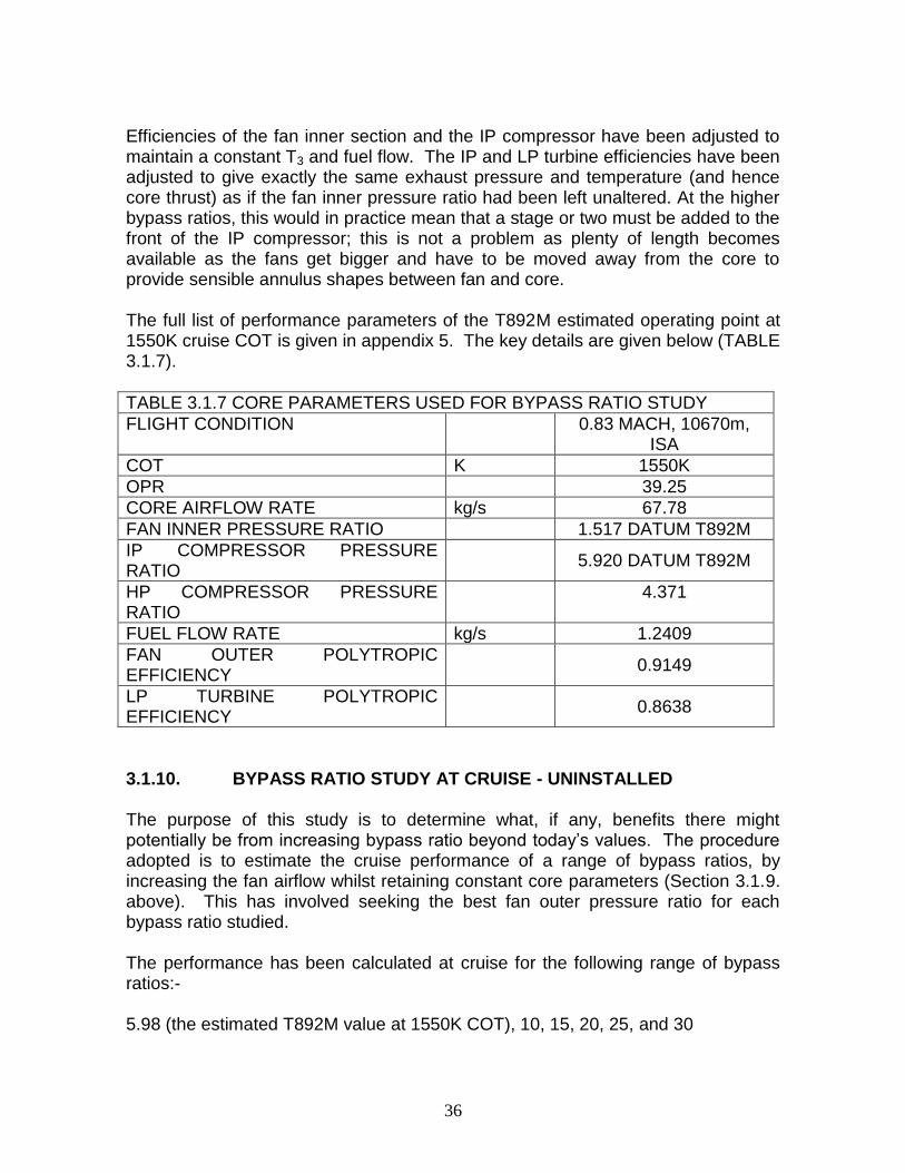
36
Efficiencies of the fan inner section and the IP compressor have been adjusted to maintain a constant T3 and fuel flow. The IP and LP turbine efficiencies have been adjusted to give exactly the same exhaust pressure and temperature (and hence core thrust) as if the fan inner pressure ratio had been left unaltered. At the higher bypass ratios, this would in practice mean that a stage or two must be added to the front of the IP compressor; this is not a problem as plenty of length becomes available as the fans get bigger and have to be moved away from the core to provide sensible annulus shapes between fan and core. The full list of performance parameters of the T892M estimated operating point at 1550K cruise COT is given in appendix 5. The key details are given below (TABLE 3.1.7).
TABLE 3.1.7 CORE PARAMETERS USED FOR BYPASS RATIO STUDY
FLIGHT CONDITION 0.83 MACH, 10670m, ISA
COT K 1550K
OPR 39.25
CORE AIRFLOW RATE kg/s 67.78
FAN INNER PRESSURE RATIO 1.517 DATUM T892M
IP COMPRESSOR PRESSURE RATIO
5.920 DATUM T892M
HP COMPRESSOR PRESSURE RATIO
4.371
FUEL FLOW RATE kg/s 1.2409
FAN OUTER POLYTROPIC EFFICIENCY
0.9149
LP TURBINE POLYTROPIC EFFICIENCY
0.8638
3.1.10. BYPASS RATIO STUDY AT CRUISE - UNINSTALLED The purpose of this study is to determine what, if any, benefits there might potentially be from increasing bypass ratio beyond today’s values. The procedure adopted is to estimate the cruise performance of a range of bypass ratios, by increasing the fan airflow whilst retaining constant core parameters (Section 3.1.9. above). This has involved seeking the best fan outer pressure ratio for each bypass ratio studied. The performance has been calculated at cruise for the following range of bypass ratios:- 5.98 (the estimated T892M value at 1550K COT), 10, 15, 20, 25, and 30

37
This range takes the study well into the region where very short cowls, open rotors and propfans may be the preferred configurations. The performance of some open rotors are calculated for comparison and presented later (Section 3.6). However, in the first part of the study, the engines’ performance is estimated to common standards, so that the point where there is need to alter the configurations at high bypass ratios can be well quantified. The performance is estimated for both the “bare engine” configuration and also, shown later, for fully installed configuration. The bare engine performance covers all thermodynamics within a control surface fronted by the fan leading edge and ended by the two nozzle planes, and covering only the air that enters the fan. The whole study is conducted for separate nozzle exhausts. A few comments are made later about mixing (Section 3.1.12.13), which in practice is only likely to be useful at the lower end of the bypass ratio range. The estimated bare engine SFC values of the full range of engines are shown on FIG 3.1.9 as a function of fan outer pressure ratio and bypass ratio.
1.1 1.2 1.3 1.4 1.5 1.6 1.7 1.8 1.913
14
15
16
17
18
19
BA
RE
EN
GIN
E S
FC
- g
/s.k
N
FAN PRESSURE RATIO
BPR 6
BPR 10
BPR 15
BPR 20
BPR 25
BPR 30
FIG 3.1.9 BARE (UNINSTALLED) SFC FOR VARYING BYPASS RATIOS AND FAN OUTER PRESSURE RATIOS; 0.83 MACH 10670m ISA; FIXED CORE; 1550K COT

38
The presence of an optimum fan outer pressure ratio for each bypass ratio is clear. It is of interest to note that even without installation losses, there is an optimum bypass ratio of about 25 with this standard of core at this flight condition. The reason that the optimum SFC at BPR 30 is worse than for BPR 25 is that the bypass duct pressure loss is becoming a dominant feature; this is explored in more detail in section 3.1.13. Checks show that the optimum fan outer pressure ratio occurs at the same value of VB/VC for every bypass ratio. This function is extremely sensitive to small changes in the fan outer pressure ratio. The optimum fan outer pressure ratio obviously falls as bypass ratio is increased; it has already been shown that at bypass ratio 5.98 (T892M value), the optimum fan outer pressure ratio is close to where the T892M is estimated to actually operate. 3.1.11 COMPARISON OF ANALYTICAL AND CALCULATED THRUST GAINS In passing it is worth comparing the augmentation of thrust due to adding a fan to a core from two sources – the analytical equations in Section 3.1.4 and the results from the design point study reported above. The numbers below are all at the appropriate optimum fan outer pressure ratios. From TABLE 3.1.2, which gave sample results from equation {16} at cruise: - (Thrust augmentation bypass ratio 20) / (Thrust augmentation at bypass ratio 6) = 1.736/1.521 = 1.141 The bare engine SFC difference at optimum fan outer pressure ratio calculated in the above study is the same as the thrust change for a fixed core (fixed fuel flow). So the SFC difference is: - (SFC of bypass ratio 6 engine) / (SFC of bypass ratio 20 engine) = 16.331 / 14.618 = 1.117 These numbers are 2.1% apart which is a remarkable agreement in view of the different ways they have been obtained. 3.1.12 CRUISE – INSTALLATION DESIGN AND LOSSES The bypass ratio study has been developed to include the effects of installation losses. The estimated installed performance includes calculated losses for the intake, cowl and afterbody. Also included are the effects of power off-takes and air off-takes for aircraft services (detailed in APPENDIX 6). Adjustments to the bypass

39
duct losses relative to the values used in the bare engine study have been made to reflect changes to the installation geometry as bypass ratio is increased. This investigation has involved considerable effort to design the aerodynamic shapes of intakes, cowls and afterbodies of several engines at each bypass ratio. The resulting long cowl installation designed by the author for the T892M is shown on FIG 3.1.10.
.
The installation aerodynamic shapes designed for all bypass ratios are shown later. The procedures used for the installation aerodynamic designs are summarised below. Full details of the geometry and loss calculations are given in APPENDIX 7. FIG 3.1.11 below shows how various installation dimensions vary with bypass ratio and fan outer pressure ratio. A method for cowl, intake and afterbody design is given by Jenkinson et al in [3.13] (1999). Its results give some confidence in the design method described below but only for lower bypass ratios. It is based on correlations of engines current in the 1980s and 1990s, which means its methods do not apply well to higher bypass ratios, and so it has not been used in this work.
FIG 3.1.10 T892M LONG COWL INSTALLATION DESIGN

40
10 15 20 25
2
4
6
FA
N T
IP
DIA
ME
TE
R -
m
10 15 20 25
5
10
14
CO
WL
LE
NG
TH
- m
LONG COWL
SHORT COWL
10 15 20 25
2
4
6
HIG
HL
IGH
T
DIA
ME
TE
R -
m
10 15 20 25
2
4
6
LP
TU
RB
INE
LE
NG
TH
- m
10 15 20 25
5
10
14
AF
TE
RB
OD
Y
LE
NG
TH
- m
LONG COWL
SHORT COWL
10 15 20 25 300
5
10
14
LP
T #
ST
AG
ES
BYPASS RATIO
FIG 3.1.11 INSTALLATION DIMENSIONS FOR VARYING BYPASS RATIOS

41
3.1.12.1 CORE DIMENSIONS A diagram of the core, to scale, is given in FIG 3.1.12 below.
The core dimensions have been taken by simple measurement of the Trent 892 from Jane’s Aero Engines [3.9]. The scale of the drawing was established from knowing the fan diameter (110ins, 2.794m) [3.9]. Full relevant engine and dimensions are given in APPENDIX 1. The leading edge of the IP compressor has been taken as the datum for axial dimensions for all the engines. 3.1.12.2 FAN DIAMETER AND INLET MACH NUMBER The diameter of the Trent 892 fan is known (2.794m) from Jane’s “Aero Engines” [3.9]. The inlet airflow of the T892M at 1550K cruise COT has been estimated using Gasturb code [3.8] and is 473.2 kg/s. The hub/tip ratio at inlet to the fan, measured from the diagram is 0.3; this has been the Rolls-Royce value for this parameter for many years. The frontal area of the fan is therefore known. Therefore the Mach number at the fan face at 1550K COT cruise can now be estimated and is found to be 0.655, an actual velocity of 198.8m/s. This value is sensible and has been kept unchanged throughout the cruise design element of the study, and is used to obtain all the fan tip diameters. Fan tip diameters of all bypass ratios are shown on FIG 3.1.11. In practice, at the higher bypass ratios, where the fan pressure ratios are low, the design fan tip speeds might be lower; this would enable the design axial velocity to be increased without significantly affecting the shock losses at the fan rotor tip.
FIG 3.1.12 T892M CORE DIMENSIONS – BASED ON RR TRENT 892 ENGINE [3.9]

42
3.1.12.3 INLET DIMENSIONS AND PRESSURE LOSS The length of the inlet from the fan leading edge has been taken as 0.5 times the fan tip diameter. This is a fairly standard number. At high bypass ratios there is a case for reducing the inlet length; this is because very high bypass ratio fans will in practice tend to have lower tip speeds and so higher fan face Mach numbers are feasible without excessive shock losses at the fan tip. This means less diffusion in the intake, which means it can be shorter. However, for this exercise, all cowled fans have been assumed, in the first instance, to have a tip speed of 400m/s at cruise design point in order to keep up the fan shaft rotational speed and so keep down the number of LP turbine stages. There are more comments on this later. The inlet total pressure ratio has been held constant at 0.998 at cruise; this is a typical value at the top end of the corrected flow range for inlets – a value nearer 0.999 might be expected at lower flows (FIG 3.1.13 – derived from [3.10]).
The fan highlight diameter has been calculated using the flight speed and an estimated inlet flow at the top of climb. The top-of-climb inlet flow has been estimated using Gasturb [3.8]. The T892M maximum climb COT has been taken as 1700K, which gives +15% thrust relative to the cruise point being used and
also gives +3% inlet airflow – all sensible numbers. A further 3% has been added to the airflow to allow for growth – a normal practice – giving 6% more inlet airflow than the T892M cruise datum point being used. The matter is not critical for this study because the highlight diameter has only a second order effect on the cowl drag estimates. Highlight diameters at other bypass ratios have been estimated using the same method. 3.1.12.4 LP TURBINE LENGTH AND NUMBER OF STAGES The total LP turbine loading (ΔH/U2) has been calculated for every engine in the study, and this has been used to calculate the number of stages and hence the turbine length. To do this, the fan tip speed has been kept constant at 400m/s and this together with the fan diameter gives the rotational speed of the LP shaft. By an iterative process it is possible to establish the outlet dimensions of the LP turbine, its mean loading, its number of stages and its total length, by making the following assumptions. The LP turbine inlet dimensions are assumed to be the
FIG 3.1.13 TYPICAL INTAKE PRESSURE RATIO [3.10]

43
same as for the RR Trent 892 engine, and the turbine outer casing hade angle has been held constant at the RR Trent 892 engine value of 25o. The loading per stage has been held constant at ΔH/U2 = 2.498 (which is close to a commonly used limit of 2.5) except for the last stage, where outlet swirl must be restrained, and where the loading is held at 1.6. These dimensions and loadings give exactly 5 LPT stages for the T892M, which is the number of stages for the RR Trent 892 engine. This method – constant loading - justifies the choice of a constant LP turbine polytropic efficiency (0.8638) for the design point study. The length per stage has been held constant at the RR Trent 892 engine value of 0.153m [3.9] and the exit hub tip ratio has been held constant at 0.5 (the lowest acceptable figure for good turbine exit root performance). The values of Va/U have been checked and found acceptable, although there is a case at very high bypass ratios for increasing the exit hub diameter of the LP turbine to increase Va and thus put Va/U into a slightly
more efficient part of the well-known “Smith chart” efficiency correlation [3.14], (FIG 3.1.14). This would not affect the LP turbine maximum diameter and therefore the installation losses would be unaltered. Note that on FIG 3.1.14, there are red points; these are locations of actual turbine test results, the details of which are not in the public domain. However, they serve to show the wide range of points in the correlation. The efficiency values on the contours are a guide only because the definitions of matters such as tip clearance are not known. However, the efficiency values given may be used for comparison purposes. As fan pressure ratio is increased at any bypass ratio the LP turbine
loading rises and more stages are needed. Also, as bypass ratio is increased, the LP shaft speed falls and this also leads to increased numbers of LP turbine stages, despite the fall in optimum fan outer pressure ratio with increasing bypass ratio. The T892M engine has 5 LP turbine stages of total length 0.765m; the optimum bypass ratio 30 engine has about 13 LP turbine stages of length about 2.02 metres. TABLE 3.1.8 below lists the numbers of LP turbine stages needed for key study cycles if there is no gear in the LP shaft. The stage numbers are not whole numbers because of the way the calculation has been done; constant stage loading and consistent turbine diameter rules have been used. The resulting turbine lengths (used in assessing the afterbody and cowl lengths) assume fractions of a stage where needed.
FIG 3.1.14 “SMITH” CORRELATION OF TURBINE EFFICIENCY [3.14] [3.15] IMAGE COURTESY ROLLS-ROYCE

44
TABLE 3.1.8 NUMBERS OF LP TURBINE STAGES
BPR 5.98 10
FOPR 1.6 1.74 1.795 1.3 1.45 1.5
LPT STAGES 4.4 4.8 5.0 5.5 6.8 7.1
BPR 15 20
FOPR 1.2 1.3 1.33 1.18 1.22 1.245
LPT STAGES 7.1 8.6 9.1 9.2 10.1 10.6
BPR 25 30
FOPR 1.1 1.18 1.195 1.1 1.15 1.162
LPT STAGES 8.8 11.6 12.0 10.6 12.8 13.2
If the fan tip speed were reduced below the 400m/s assumed at all bypass ratios, the number of LP turbine stages would increase approximately as the square of the inverse of the fan tip speed; for example, if the fan tip speed were reduced to 350m/s, the number of LP turbine stages would rise from 13 to 17 at bypass ratio 30. There is obviously a clear need to consider a gearbox in the fan shaft. P&W have recently offered a geared fan engine, the PW 1000G (BPR about 10). 3.1.12.5 LONG COWL DIMENSIONS AND LOSSES The fan cowl maximum thickness is taken as 0.25 m for all engines. This allows room for the accessory pack, front mount and certain aircraft services. Thus the cowl maximum diameter is 0.5m greater than the fan tip diameter in each case. The inlet leading edge is 0.5 times the fan diameter from the fan front face (see 3.1.12.3). The fan axial position moves forward as bypass ratio increases. This is because there must be enough room for the core air to turn into the core from the exit of the fan inner section. Since the fan root dimension increases with increasing bypass ratio, more length is required. It is assumed that the passage into the core retains its current outer hade angle of 10o (see FIG 3.1.12 above). A smooth variation of the fan axial distance from the core can now be established. A smooth variation of fan aspect ratio with bypass ratio is also used. These rules set the fan leading edge axial position, and hence the axial dimension of the inlet leading edge in relation to the core. The long cowl trailing edge, which is the bypass nozzle exit plane, is assumed to be axially coincident with the trailing edge of the strut behind the LP turbine. The LP turbine length has been set as above. The rear strut trailing edge is assumed to have an axial position 0.5m downstream of the LP turbine trailing edge. Thus the length of the cowl and its maximum diameter are both known. The cowl is assumed to be cylindrical except where it needs to fair into the inlet and bypass nozzle curvatures.

45
The bypass nozzle area is known from the cycle of each engine. For the long cowl, the inner radius is assumed to be a certain amount “x” larger than the LP turbine maximum (exit) radius. This allows for a strong ring in the turbine casing to carry rear mount loads through to the rear LP turbine bearing. The amount “x” is graded from 0.1m at bypass ratio 5.98 to 0.15m at bypass ratio 30. Thus the bypass nozzle outer diameter can be calculated. The boat-tail angle of the cowl is a typical 11o. The dimension over the LP turbine exit is maintained as the afterbody diameter for the short cowl configuration upstream of the LP turbine. Short cowl design methods are given in SECTION 3.1.12.12. The cowl drag at cruise has been calculated using the method of Walsh and Fletcher [2.6]. It is a simple method using loss coefficient, dynamic head and wetted area. The loss coefficient used is the recommended 0.003 and a reasonable interference factor of 1.2 has been assumed. The cowl cruise drag for the T892M is 3.04% of net thrust. Variation of cowl drag with bypass ratio is shown on FIG 3.1.15 below for both long and short cowls.
1.1 1.2 1.3 1.4 1.5 1.6 1.7 1.8 1.9
2
4
6
8
10
DR
AG
- kN
SHORT COWL ENGINE
1.1 1.2 1.3 1.4 1.5 1.6 1.7 1.8 1.90
2
4
6
8
10
DR
AG
- kN
LONG COWL ENGINE
1.1 1.2 1.3 1.4 1.5 1.6 1.7 1.8 1.90
2
4
6
8
10
12
% N
ET
THR
US
T
FAN PRESSURE RATIO
BPR 6BPR 10BPR 15BPR 20BPR 25BPR 30LONG COWL ENGINESHORT COWL ENGINE
FIG 3.1.15 COWL DRAG FOR VARYING BYPASS RATIO AND FAN PRESSURE RATIO; 0.83 MACH, 10670m, ISA; FIXED CORE, 1550K COT

46
3.1.12.6 AFTERBODY The area of the core final nozzle is known, giving its diameter. The boat-tail angle of the afterbody is a conventional 14o. The afterbody shape immediately downstream of the bypass nozzle trailing edge is assumed to be cylindrical. The core nozzle diameter is known; thus, by drawing, it is possible to create the shape of the afterbody to a reasonable accuracy. Variations in length with bypass ratio are shown on FIG 3.1.11. It is assumed that there is no turbine cone protruding from the core nozzle. This is not the case for the actual RR Trent 892 powerplant, which has a protruding cone (FIG 3.1.16). The addition of a turbine cone reduces the afterbody losses slightly at the expense of additional losses due to high speed flow over the cone itself. For the sake of this study, this matter is not important as the net change in loss is small. So the complication of estimating the cone losses has been avoided for simplicity.
The afterbody drags have been calculated by the same Walsh and Fletcher method as for the cowl [2.6]. The Mach number over the afterbody has been calculated at the bypass nozzle trailing edge and assumed unchanged along the afterbody for the purposes of assessing its drag. The mean afterbody diameter and its length have been used to obtain the wetted area. FIGS 3.1.17 and 3.1.18 show examples of the effects of bypass ratio and fan outer pressure ratio on afterbody shape.
FIG 3.1.16 COWLING OF RR TRENT 892 POWERPLANT SHOWING PROTRUDING TAIL CONE Image Courtesy Rolls-Royce

47
Long cowl afterbody drags vary from about 2.1% of net thrust at bypass ratio 5.98 to 2.3% at bypass ratio 30 (where the lower Mach number of the bypass flow is more than offset by the added afterbody length to accommodate the LP turbine) Results for long and short cowl installations are shown on FIG 3.1.19. Short cowl afterbody drags are naturally much higher.
FIGS 3.1.17 SAMPLE EXHAUST GEOMETRIES, BPR 5.98
FIG 3.1.18 SAMPLE EXHAUST GEOMETRIES, BPR 20

48
1.1 1.2 1.3 1.4 1.5 1.6 1.7 1.8 1.9
1
2
3
4
5
DR
AG
- k
N
1.1 1.2 1.3 1.4 1.5 1.6 1.7 1.8 1.90
1
2
3
4
5
6
% N
ET
TH
RU
ST
FAN PRESSURE RATIO
BPR 6BPR 10BPR 15BPR 20BPR 25BPR 30LONG COWL ENGINESHORT COWL ENGINE
3.1.12.7 TOTAL DRAG Long cowl installations: for long cowl installations, the calculated total pod (cowl plus afterbody) drags vary from about 5% of net bare engine thrust at bypass ratio 5.98 to about 13% at bypass ratio 30 (FIG 3.1.20). Two curves showing the total drag of the cowl and afterbody as percentages of both bare and installed thrust (from APPENDICES 7 and 9 respectively) are plotted against specific thrust on FIG 3.1.21, where they are compared with estimates made in 1973 by Mr. Hatton of Rolls-Royce, and published by the author as lecture notes [3.10]. The general shape and level of the three curves is remarkably similar, giving confidence in the methods used herein. Short cowl installations: for short cowl installations the total pod drag is about 2% higher than for the long cowl case at bypass ratio 5.98 due to the high Mach number of the bypass flow over the large afterbody area. However, at bypass ratio 30, where the Mach number is lower and the area not much greater, the total pod drag is about 2% less than for the long cowl (see FIG 3.1.20).
FIG 3.1.19 AFTERBODY DRAG FOR VARYING BYPASS RATIO AND FAN PRESSURE RATIO; 0.83 MACH, 10670m, ISA; FIXED CORE 1550K COT

49
1.1 1.2 1.3 1.4 1.5 1.6 1.7 1.8 1.9
4
6
8
10
12D
RA
G -
kN
SHORT COWL ENGINES
1.1 1.2 1.3 1.4 1.5 1.6 1.7 1.8 1.9
6
8
10
12
14
% N
ET
TH
RU
ST
SHORT COWL ENGINES
1.1 1.2 1.3 1.4 1.5 1.6 1.7 1.8 1.9
4
6
8
10
12
DR
AG
- k
N
LONG COWL ENGINES
1.1 1.2 1.3 1.4 1.5 1.6 1.7 1.8 1.94
6
8
10
12
14
% N
ET
TH
RU
ST
FAN PRESSURE RATIO
BPR 6
BPR 10
BPR 15
BPR 20
BPR 25
BPR 30
LONG COWL ENGINES
FIG 3.1.20 TOTAL POD DRAG (COWL + AFTERBODY); VARYING BYPASS RATIO, FAN PRESSURE RATIO; 0.83 MACH, 10670m, ISA; FIXED CORE, 1550KCOT. % OF BARE THRUST (APPENDIX 7)

50
30 50 70 90 110 130 150 170 190 210 2300
2
4
6
8
10
12
14
16
18
PO
D D
RA
G %
NE
T T
HR
US
T
SPECIFIC THRUST N/(kg/s)
BPR 6
BPR 10
BPR 15
BPR 20
BPR 25
BPR 30
ESTIMATE FROM ATTACHMENT 1
RESULTS USING BARE ENGINE THRUST (APP 7)
RESULTS USING INSTALLED THRUST (APP 9)
3.1.12.8 BYPASS DUCT From the cowl design method described above, the bypass duct exit dimensions are known. The axial position of the inlet to the bypass duct is assumed to be the trailing edge of the fan bypass OGV. The axial position of this plane moves smoothly forward by a small amount as bypass ratio increases. The bypass duct entry outer diameter is assumed to be the same as that of the fan rotor exit. This dimension is determined by consideration of the fan exit Mach number and actual axial velocity. It is found that as bypass ratio increases and fan outer pressure ratio falls, it is necessary to increase the bypass duct velocity to maintain a sensible shape of fan outer casing and a sensible bypass duct inner radius. It increases from 140m/s at bypass ratio 5.98 to about 178m/s at bypass ratio 30; comparing these figures with the fan inlet axial velocity of 195.6m/s shows a satisfactory situation as some diffusion of axial velocity in not unusual in fan aerodynamic design. The bypass duct inner radius determines the position of the splitter – where the inner radius meets the (10o) angled duct to the core is the location of the splitter leading edge. This then helps to place the fan trailing edge axially. Spacing between fan rotor and OGV increases smoothly with bypass ratio.
FIG 3.1.21 COMPARISONS OF TOTAL POD DRAG WITH SPECIFIC THRUST – LONG COWL (REF [3.10].) 0.83 MACH, 10670m, ISA; FIXED CORE, 1550K COT

51
The bypass duct loss is estimated using the flow dynamic head, the wetted area and an equivalent loss coefficient and then dividing by the flow. The equivalent coefficient has been obtained by assuming the bypass loss of the T892M is 1.5% total pressure at the model design point at take-off. At 1550K cruise COT this becomes 1.508%. Long cowl bypass duct loss has fallen to about 1.21% at bypass ratio 30 due to the much larger hydraulic mean depth, despite higher duct velocities (FIG 3.1.22). Short cowl bypass loss is obviously much lower.
1.1 1.2 1.3 1.4 1.5 1.6 1.7 1.8 1.90
0.1
0.2
0.3
0.4
0.5
0.6
0.7
0.8
0.9
1
1.1
1.2
1.3
1.4
1.5
1.6
% D
elt
aP
/P
FAN PRESSURE RATIO
BPR 6BPR 10BPR 15BPR 20BPR 25BPR 30LONG COWL ENGINESHORT COWL ENGINE
3.1.12.9 POWER OFFTAKE The power off-take at cruise is used for creating hydraulic pressure for the aircraft controls and electrical energy for aircraft services. Typical figures have been supplied by Laskaridis [3.16] and these agree with earlier findings by the author [3.17]. The maximum power off-take designed-in is approximately 0.001kW/kgMTOW. The B777 is about 300,000kg MTOW giving 300kW, or 150kW per engine. Normal use is 70% of this so 110kW has been taken. This has been scaled as necessary to reflect the increases in cruise net thrust of the higher bypass engines (tacitly assuming therefore that more thrust will drive a heavier aircraft with more passengers).
FIG 3.1.22 BYPASS DUCT LOSS VARIATION WITH BYPASS RATIO AND FAN PRESSURE RATIO; 0.83 MACH, 10670m, ISA; FIXED CORE, 1550K COT

52
3.1.12.10 AIR OFFTAKE Normal air requirement for cabin conditioning is about 1lb/min per person. Assuming for the B777 the maximum seating of 550 and 10 crew gives 2.12kg/s per engine. This has been rounded up to 2.15 and then suitably scaled by cruise thrust for the higher bypass ratio engines. Details of the air and power off-takes are given in APPENDIX 6. 3.1.12.11 DIMENSIONS AND RESULTS The details of all the installation loss calculations are given in APPENDIX 7. All the relevant dimensions of the various installation designs are summarised in APPENDIX 8. FIG 3.1.23 compares the long and sort cowl nacelles of the various bypass ratios for the optimum fan pressure ratios in each case. 3.1.12.12 SHORT COWL DESIGN AND PERFORMANCE It is clear that the performance losses associated with the fan cowl, the afterbody and bypass duct are significant particularly at the higher bypass ratios (TABLE 3.1.9). This is discussed more fully later. So, short fan cowls have been designed for all engines in the bypass ratio study, and the losses estimated. The length of each short cowl has been taken as equal to the maximum diameter of the cowl (L/D = 1.0). The core nozzle position and the inlet shapes are assumed unaltered. The afterbody average diameter for each engine has been taken as 1.1 times the average diameter of the afterbody for the long cowl engine. The velocity of the bypass nozzle exhaust is assumed, as was the case for the long cowls, to apply over the whole of the afterbody. The bypass loss has been reduced in proportion to the length reduction of the bypass duct.

53
3.1.12.13 MIXED EXHAUSTS Mixing the bypass and core exhaust flows in a common jet pipe can potentially give useful performance improvements – of the order 2 to 4% of cruise SFC [2.6] [3.10] for bypass ratios around 4 to 6. These gains come from improvements in propulsive efficiency arising naturally from the more uniform distribution of exhaust flow temperature [3.10]. However, as design bypass ratio is increased, the performance gains reduce as the core jet temperature falls. Furthermore the weight of the cowl becomes prohibitive bearing in mind the need for a reverser and, at bypass ratios above about 12, there is a need to use a variable bypass nozzle for fan performance stability. Thus, for the studies reported herein, the option of exhaust mixing is not considered further.
FIG 3.1.23 LONG AND SHORT COWL DESIGNS

54
3.1.13. CRUISE BYPASS RATIO STUDY – INSTALLED PERFORMANCE Installation losses at cruise have been calculated as indicated in the previous section and applied to the full range of bypass ratios. The full details of the intake, bypass duct, cowl and afterbody loss calculations are shown in APPENDIX 7. The detailed effects on each engine of each of these installation losses together with the effects of power and air off-takes are shown on the table in APPENDIX 9. The effects of air and power off-takes have been calculated using Gasturb code [3.8]. The individual effects of the various long cowl installation losses are summarised in TABLE 3.1.9 below for the optimum bare engine fan outer pressure ratio in each case.
TABLE 3.1.9
CHANGES IN SFC DUE TO INSTALLATION LOSSES - LONG COWLS; 0.83 MACH, 10670m, ISA %SFC
BYPASS RATIO/ SPECIFIC THRUST
5.98 (T892M)
160.1
10
108.5
15
76.9
20
59.0
25
48.0
30
40.1
FAN PR 1.795 1.5 1.33 1.245 1.195 1.162
INTAKE LOSS 0.998
0.23 0.37 0.56 0.75 0.95 1.16
POWER OFFTAKE
0.34 0.42 0.46 0.48 0.50 0.51
AIR OFFTAKE
4.01 6.02 7.27 8.05 8.76 9.34
BYPASS DUCT LOSS CHANGE
0.00 -0.15 -0.41 -0.76 -1.29 -1.84
AFTER -BODY DRAG
2.35 2.21 2.20 2.38 2.54 2.78
LONG COWL DRAG
3.52 5.32 7.47 9.67 11.86 14.53
TOTAL SFC CHANGE %
10.82 14.86 18.54 21.88 24.93 28.46
Note that the afterbody and cowl drag SFC changes shown are consistent with APPENDIX 9 – they are percentages of installed thrust. The major losses are due to the drag of the long fan cowl and the air off-take for cabin pressurisation. The total installation loss for the T892M is about 10.8% whereas at bypass ratios 15 and 30 the total installation losses are about 18.5% and 28.5% respectively (massive losses).
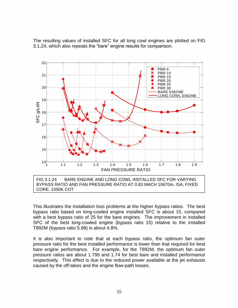
55
The resulting values of installed SFC for all long cowl engines are plotted on FIG 3.1.24, which also repeats the “bare” engine results for comparison.
1 1.1 1.2 1.3 1.4 1.5 1.6 1.7 1.8 1.914
15
16
17
18
19
20
21
22
SF
C g
/s.k
N
FAN PRESSURE RATIO
PBR 6PBR 10PBR 15PBR 20PBR 25PBR 30BARE ENGINELONG COWL ENGINE
This illustrates the installation loss problems at the higher bypass ratios. The best bypass ratio based on long-cowled engine installed SFC is about 15, compared with a best bypass ratio of 25 for the bare engines. The improvement in installed SFC of the best long-cowled engine (bypass ratio 15) relative to the installed T892M (bypass ratio 5.98) is about 4.8%. It is also important to note that at each bypass ratio, the optimum fan outer pressure ratio for the best installed performance is lower than that required for best bare engine performance. For example, for the T892M, the optimum fan outer pressure ratios are about 1.795 and 1.74 for best bare and installed performance respectively. This effect is due to the reduced power available at the jet exhausts caused by the off-takes and the engine flow-path losses.
FIG 3.1.24 BARE ENGINE AND LONG COWL INSTALLED SFC FOR VARYING BYPASS RATIO AND FAN PRESSURE RATIO AT 0.83 MACH 10670m, ISA; FIXED CORE, 1550K COT

56
Also, at the higher bypass ratios the range of fan outer pressure ratios that might be acceptable is much narrower than at the lower bypass ratios. At 15 bypass ratio, a penalty in SFC of less than 1% relative to optimum covers a range of fan outer pressure ratios of only 1.26 to 1.325. It is therefore crucial to be sure of the fan design parameters if the benefits of high bypass ratio are to be realised. Put another way, the installed SFC at 15 bypass ratio with a fan outer pressure ratio of 1.325 is the same as at bypass ratio 10 with a fan outer pressure ratio of 1.43. The bypass 10 engine would be lighter and easier to install and have fewer LP turbine stages. Furthermore the engine of bypass ratio 10 would probably not suffer from fan instability problems at take-off and would not need a variable bypass nozzle. In the present study, the potential long cowl installed SFC benefit of bypass ratio 15 relative to 10 is only about 0.8%. These effects are well known to the industry and are also discussed in various ways in the literature [2.4], [2.5], [2.6], [3.10], [3.18] and [3.19]. However, it is of interest to repeat the calculations from time to time to incorporate the effects of improving engine and installation technologies. The present study uses modern technology standards, particularly in respect of OPR and COT levels at cruise. The effects of even higher COT, OPR and component efficiencies are discussed shortly. The most thorough installed performance study found in the literature is Zimbrick and Colehour’s 1988 paper to AIAA [3.18]. They concluded that, with the core they had used, there was little point in choosing a bypass ratio higher than 9.6, because although there was, for their assumptions, theoretically 3 to 4% better installed SFC available at bypass ratio 17, the increased mechanical complexity and maintenance cost would probably not make such an engine worthwhile. However, they had used a TET (at turbine rotor inlet) of 1388K, equivalent to a COT of perhaps about 1450K. They did not explore weight effects although they did discuss short cowls. They explored fan designs and discussed the problem of thrust reversing methods. It is very clear at this point why there has been, and still is interest in short cowls, open rotors and propfans. If a propfan or open rotor could be developed that was capable of operation at 0.8 Mach cruise, was efficient and had low noise at take-off it would reap the benefits from having no cowl drag, no intake loss and no bypass duct loss. Afterbody drag would increase but there would be a net performance benefit. Open rotors and propfans are considered in Section 3.6. Short cowls offer the advantages of some reduction in installation losses, but they have less room for sound absorbing linings in their bypass ducts and so are potentially noisier. Short cowl and long cowl installed SFCs are compared in the TABLE 3.1.10 below and also on FIG 3.1.25.

57
TABLE 3.1.10 SFC CHANGES DUE TO INSTALLATION LOSSES; SHORT –v- LONG COWLS 0.83 MACH, 10670m, ISA %SFC
BYPASS RATIO/ SPECIFIC THRUST
5.98 (T892M)
160.1
10
108.5
15
76.9
20
59.0
25
48.0
30
40.1
INTAKE LOSS 0.998
0 0 0 0 0 0
POWER OFFTAKE
0 0 0 0 0 0
AIR OFFTAKE 0 0 0 0 0 0
BYPASS DUCT LOSS REL LONG
-0.91 -1.73 -2.64 -3.58 -4.42 -5.42
AFTERBODY DRAG REL LONG
2.73 2.93 2.76 2.91 2.96 3.35
COWL DRAG REL LONG
-1.37 -2.27 -3.30 -4.35 -5.36 -6.81
TOTAL % SFC CHANGE SHORT COWL
11.26 13.60 14.88 16.04 16.91 17.87
TOTAL % SFC CHANGE LONG COWL
10.82 14.86 18.54 21.88 24.93 28.46
% SFC LOSS DIFFERENCE SHORT – LONG COWLS
0.44 -1.26 -3.66 -5.84 -8.02 -10.59
The clear conclusion from the above table is that the short cowl offers no installation performance benefit at bypass ratios up to about 8. At higher bypass ratios, the short cowl offers lower installation losses than the long cowl. Although the short cowl has a larger afterbody drag, the fan cowl drag and bypass duct losses are much reduced relative to the long cowl. FIG 3.1.25 illustrates the result and shows also the effect of varying fan outer pressure ratio at each bypass ratio. It can also be clearly seen that the optimum bypass ratio is higher for short cowls than for long ones. The optimum fan outer pressure ratio is fractionally lower for short cowls than long cowls at any bypass ratio. Also shown on FIG 3.1.25, for interest, are the installed SFC results for the open rotors, which use the T892M core like the main study engines. The open rotors are discussed in full in Section 3.6.

58
1 1.1 1.2 1.3 1.4 1.5 1.6 1.7 1.815
16
17
18
19
20
21
SF
C -
g/s
.kN
FAN PRESSURE RATIO
BPR 6BPR 10BPR 15BPR 20BPR 25BPR 30SHORT COWL ENGINESLONG COWL ENGINEsPropfan BPR 30Propfan BPR 50Propfan BPR 80
It must be observed at this point that although the short cowl offers potential performance advantages over long cowls, they are inherently noisier as there is less length in the bypass duct in which to install sound absorbent linings. There is also the issue of providing a thrust reverser. 3.1.14 PERFORMANCE EXCHANGE RATES The results presented so far cover attempts at achieving better installed cruise SFC by improving propulsive efficiency using changes to bypass ratio and fan pressure ratio, all at constant component efficiencies. Using these methods, which are aimed at improving propulsive efficiency, there are obviously difficulties in finding even 5% better installed SFC relative to the T892M. Therefore, to set these results in context, can improvements to component efficiencies and core cycle parameters at cruise yield better gains? The table below (TABLE 3.1.11) summarises the effects on SFC of small changes in component quality, measured by efficiencies or losses, for bypass ratios of 5.98 (T892M) and 20 at cruise. Full details, including the effects on thrust, are given in APPENDIX 10. COT and OPR have been kept constant, but are investigated in the next section.
FIG 3.1.25 SHORT COWL, LONG COWL AND OPEN ROTOR INSTALLED SFC VARIATION WITH BYPASS RATIO AND FAN PRESSURE RATIO AT 0.83 MACH, 10670m, ISA; FIXED CORE, 1550K COT

59
TABLE 3.1.11 PERFORMANCE EXCHANGE RATES 0.83 MACH 10670m ISA
BYPASS RATIO 5.98 20
Change ΔSFC % ΔSFC %
Fan outer efficiency +1% -0.45 -0.75
Fan inner efficiency +1% -0.07 -0.11
IP compressor efficiency +1% -0.30 -0.47
HP compressor efficiency +1% -0.27 -0.42
Combustor ΔP/P -1% -0.30 -0.37
HP turbine efficiency +1% -0.38 -0.46
IP turbine efficiency +1% -0.30 -0.37
LP turbine efficiency +1% -0.60 -0.91
Bypass duct ΔP/P -1% -0.82 -3.25
Core nozzle thrust coefficient +1% -0.44 -0.30
Bypass nozzle thrust coefficient +1% -1.72 -5.01
The strong influence of the fan outer efficiency, the LP turbine efficiency, the bypass duct loss and the bypass nozzle coefficient are evident. All efficiencies and losses have greater influence at bypass ratio 20 than at bypass ratio 5.98. Although the influence of the bypass nozzle thrust coefficient is enormous at bypass ratio 20, it should be noted that a (typical) value of 0.999 has been used throughout this study for the thrust coefficient of each nozzle, and so the scope for improving SFC by improving thrust coefficient is small. Conversely, if the nozzle aerodynamic shapes were poorly designed, there could be large performance losses. If it were postulated that a 1% improvement in turbo-machinery efficiencies together with a 1% reduction in combustor and bypass duct pressure loss became available from technology research, the SFC of the bypass ratio 5.98 and 20 engines would improve by 3.49% and 7.11% respectively, a difference of 3.62%. This would make the installed SFC of the bypass ratio 20 engine about 7.4% better than bypass ratio 5.985, instead of only 3.8% better. The bulk of the difference is caused by the different influences of the bypass duct loss, which points to reducing the bypass duct length as a possible means of improving installed SFC. If the bypass duct loss is excluded from consideration in the above analysis, the SFC gain of the bypass 20 engine relative to the gain at bypass ratio 5.98 is only 1.2% from the turbo-machinery and combustor improvements postulated. 3.1.15 EFFECTS OF CHANGING CORE PARAMETERS So far, for the entire design point study into the effects of bypass ratio and fan outer pressure ratio, the core parameters have been kept constant. Since the pursuit of better (lower) SFC by increasing the design bypass ratio is to some extent thwarted by installation losses, a short study is now presented which explores the effects of changes to the core performance. The above section shows the effects of changes to the component efficiencies including those in the

60
core. This section therefore covers only changes to the overall pressure ratio (OPR) and Combustor Outlet Temperature (COT). Design points at cruise have been calculated for all combinations of the following ranges of parameters, in order to show the effects at various bypass ratios of changes to OPR and COT. For each combination, the optimum fan outer pressure ratio has been determined. The results shown (FIG 3.1.26) are for bare (uninstalled) engine performance in order to show the cleanest cycle effect; however, the effects will be similar for the installed engines. Bypass ratios: 5.985 (base), 10, 20 and 30 OPR 39.2 and 43.08 (datum and +10%) COT 1550K and 1650K (datum and +100oK)
1.1 1.2 1.3 1.4 1.5 1.6 1.7 1.8 1.9 2
14.5
15
15.5
16
16.5
17
FAN PRESSURE RATIO
UN
INS
TA
LL
ED
SF
C -
g/(
s.k
N)
COT=1550 & OPR=39
COT=1550 & OPR=43
COT=1650 & OPR=39
COT=1650 & OPR=43
BPR 6
BPR 10
BPR 20
BPR 30
FIG 3.1.26 UNINSTALLED SFC VARIATIONS FROM CORE OPR AND COT CHANGES

61
The effect of increasing OPR by 10% is to improve SFC by about 0.5 to 1% depending on details of the other cycle parameters. This effect is a combination of gains in thermal and propulsive efficiencies. The thermal efficiency gain is to be expected – a simple Froude cycle effect. The propulsive efficiency gain is due, of course, to a fall in jet velocities. Increasing OPR raises T3 and hence the combustor temperature rise is less; this leads to reduced fuel flow and so there is less energy to drive the LP turbine, so less power to the fan. Another consequence is that optimum fan outer pressure ratio falls. Changing the OPR makes little difference to making the best choice of bypass ratio. The effect of increasing the COT by 100K is to worsen SFC at lower bypass ratio but improve it at higher bypass ratio. Increasing COT by 100K improves core thermal efficiency slightly (around 1.5%). However, at the lower bypass ratios (5.98 and 10), this small gain in thermal efficiency is more than offset by a loss of propulsive efficiency, which results from the extra energy leaving the engine in the form of higher jet velocities. At the higher bypass ratios (20, 30) the extra energy available to drive the LP turbine and the fan still worsens the propulsive efficiency, but because the optimum fan outer pressure ratio rises with increased COT, the influence of bypass duct loss is less strong; in effect the thermal efficiency, measured by the kinetic energy gains in the two streams, is enhanced. These effects cause the optimum bypass ratio to increase; as can be seen on FIG 3.1.26, the locus of optimum SFC does not reach an optimum at COT 1650K until at least bypass ratio 30, whereas at 1550K, there is a clear best bypass ratio around 20. The SFC at bypass ratio 30 is improved by over 2% by increasing COT to 1650K. Thus, to take advantage of the benefits of high bypass ratio, the core energy output should be maximised. 3.1.16 PERFORMANCE AT TAKE-OFF The study presented so far has concentrated on seeking the best cruise installed SFC by examining the effects of varying bypass ratios, fan outer pressure ratios, component efficiencies, OPR, COT and installation configurations. The potential improvements in installed SFC relative to a “Base Engine” (the T892M) have been quantified for long and short cowled engines. Open rotors and propfans will be considered in Section 3.6. The purpose of the next part of the study is to explore the take-off performance of the long-cowled range of engines, (which will be very similar for the short cowled engines), and to provide engine data for use in noise estimation, which will be presented in Section 3.2. Off-design calculations have been made to estimate installed take-off performance, which is presented at SL, 0.2 Mach ISA and at SL Static ISA. The main study is at 0.2 Mach because this is a critical condition for airport noise and because this is also a critical point for aircraft take-off. As will be shown, the net thrust of any engine falls significantly during the take-off run, and this effect is greatest at the

62
higher bypass ratios (lowest specific thrusts). At the higher bypass ratios, increases in bypass nozzle areas are required for fan stability reasons. This is explained in Section 3.1.16 below. The assumptions made in calculating the installation losses are as follows.
Cowl and afterbody dimensions are the same as for cruise – it has been assumed that the fitting of a variable bypass nozzle area (discussed below) does not affect the cowl wetted area significantly. Intake pressure ratio = 0.995 Power and air off-takes the same absolute values as for cruise
The TABLE 3.1.12 below shows the values of long cowl drag and afterbody drag as percentages of the engine net thrust at 0.2 Mach number, sea level, ISA.
TABLE 3.1.12 LONG COWL AND AFTERBODY DRAGS 0.2MACH TAKE-OFF S.L. ISA
NOMINAL BYPASS RATIO 5.98 10 20 30
FAN DESIGN PRESSURE RATIO 1.74 1.45 1.22 1.15
COWL DRAG % THRUST 0.17 0.23 0.34 0.44
AFTERBODY DRAG % THRUST 0.83 0.65 0.47 0.38
The ratio of installed take-off thrust to installed cruise thrust at fixed COT is shown for all bypass ratios in TABLE 3.1.13 below. Also shown is the take-off COT of each engine that is required to achieve the datum (T892M) ratio of take-off to cruise thrusts. The results are repeated as a graph on FIG 3.1.27. TABLE 3.1.13 TAKE-OFF AND CRUISE INSTALLED PERFORMANCE; LONG COWL
CRUISE 0.83M 10.67km ISA
TAKE-OFF Bypass Nozzle %
TAKE-OFF SLS ISA TAKE-OFF SL 0.2M ISA
TO Fn 0.2M / 0.0M
BPR FPR COT
K
Fn kN INST
COT K
Fn kN INST
FnTO / Fn cr
COT K
Fn kN INST
FnTO / Fn cr
5.98 1.74 1550 66.0 DATUM 1795 390.6 5.91 1795 325.3 4.92 0.83
10 1.45 1550 68.7 5% 1795 482.4 7.03 1795 380.4 5.54 0.79
5% 1624 406.1 5.91 1680 338.1 4.92 0.83
20 1.22 1550 68.3 18% 1795 634.3 9.29 1795 461.7 6.76 0.73
18% 1468 404.1 5.91 1563 336.2 4.92 0.83
30 1.15 1550 65.2 38% 1795 752.8 11.55 1795 504.7 7.74 0.67
38% 1390 385.6 5.91 1501 321.0 4.92 0.83

63
It is clear that the higher bypass ratio engines can produce vastly more take-off thrust in relation to cruise thrust than those with lower bypass ratios.
3.1.17 FAN OPERATING STABILITY AT TAKE-OFF When a turbofan engine designed at cruise with a low fan pressure ratio is operated at take-off, there is a significant rise in the fan working line level between cruise and take-off. The lower the design fan pressure ratio the more marked is the effect. The effect is caused by the reduction in forward speed between cruise and take-off, which reduces the effective capacity (W√T/P) of the unchoked bypass nozzle because of the lower nozzle pressure ratio. The effect is not present if the fan design pressure ratio is high enough that at take-off the bypass nozzle remains choked (such as on very low bypass ratio military engines). However, for the full range of engines being explored herein, the effect is present. To explain the shift in working line between cruise and take-off, consider a simple fan operating with a final nozzle, without complications of a core flow (a fan on rig test can be envisaged); FIG 3.1.28.
10 15 20 254
6
8
10
12
5 10 15 20 25 30
1400
1500
1600
1700
1800
CO
T -
K
DESIGN BPR
MACH 0
MACH 0.2
CONST. COT=1794.5 K
CONST. TAKE-OFF/CRUISE THRUST
FIG 3.1.27 SL TAKE-OFF COT AND THRUST CHANGES WITH BPR; LONG COWL
CR Fn
FnT/O

64
The shift in working line between take-off and cruise is due to the nozzle flow capacity (W√T/P)2 reducing as the nozzle unchokes. Let the fan operate at the same value of inlet (W√T/P)1 at two flight conditions, namely SLS ISA (take-off) and 0.83 Mach 10670m ISA (cruise). Let the fan efficiency remain constant at 0.88 polytropic. The final nozzle area remains constant. Let the design fan pressure ratio at cruise be 1.3 (appropriate to high bypass ratio – about 15 to 20 in this study). The objective is to determine the fan operating pressure ratio at take-off. At fixed (W√T/P)1 this will show the shift in working line level. The results are in TABLE 3.1.14, below. At take-off, the fan (outer) pressure ratio rises to 1.42 at fixed inlet (W√T/P)1, a 40% increase in pressure rise. This large change would almost certainly lead to surge at take-off.
TABLE 3.1.14 FAN WORKING LINE SHIFT CRUISE TO TAKE-OFF
UNITS CRUISE 0.83M 10670km ISA
TAKE-OFF SLS ISA
P1 kPa 37.45 101.33
T1 K 248.9 288.15
Flight Mach 0.83 0
P1 / p0 1.571 1.0
Inlet Airflow kg/s 100 251.6
(W√T/P)1 0.04213 0.04213
P2 / P1 1.3 1.42
P2 / p0 2.042 1.42
Mach Nozzle (2) 1.0 0.726
(W√T/P)2 0.03382 0.03142
Area2 (Nozzle) m^2 0.8368 0.8368
p0
1
2
FIG 3.1.28 FAN WORKING LINE CONTROL; BYPASS NOZZLE AREA CHANGE
TAKE OFF
CRUISE
FAN

65
3.1.18 BYPASS NOZZLE AREA CHANGES AT TAKE-OFF There are two well-known methods of countering the fan working line problem at high bypass ratio (i.e. low fan pressure ratio):- “Fining” the fan blade pitch angle Increasing bypass nozzle area Varying the pitch angle is a technology well known in the propeller field, and it can be employed successfully in high bypass ratio turbofans up to a point. The effect of varying pitch (to “finer” at take-off) is to shift the standard fan characteristic (e.g. FIG 3.1.30) bodily to lower flows at any given rotational speed. There is usually a small loss in surge pressure ratio at a rotational speed. Therefore the technique is limited to cases where the shift in fan working line is not very large – that is to say cases where the fan design pressure ratio is not extremely low. Varying the bypass final nozzle area is wholly effective in eliminating fan flow instability at take-off if sufficient increase in area can be provided. This method of achieving fan flow stability has been selected for this study. The amount of the bypass nozzle area increase required is a function of the fan pressure ratio. In the present study, the bypass nozzle area increases chosen are such as to place the take-off working points at 0.2 Mach number, sea level, at about the same working line level as the cruise operating point on the fan performance characteristics for each engine. The changes are shown on FIG 3.1.29 and provide sufficient surge margin to allow for the further rise in fan working line between 0.2 and 0 Mach numbers, sea, level.
1 1.1 1.2 1.3 1.4 1.5 1.6 1.7 1.8 1.90
10
20
30
40
50
60
70
BY
PA
SS
NO
ZZ
LE
AR
EA
VA
RIA
TIO
N %
FAN PRESSURE RATIO
BPR 6
BPR 10
BPR 15
BPR 20
BPR 25
BPR 30
FIG 3.1.29 VARIATION IN BYPASS NOZZLE AREA AT TAKE-OFF

66
As an example, the cruise and take-off operating points on the fan characteristic are shown in FIG 3.1.30 below for the most extreme example considered (bypass ratio 30 with fan design pressure ratio 1.1). Clearly the engine cannot be operated at take-off with the cruise bypass nozzle area because the fan flow would be highly unstable. Even at bypass ratio 10 in the present study, there is a slight risk of fan instability, and so small increases in bypass nozzle area have been applied (FIG 3.1.29 above). At bypass ratio 6, sufficient margin can be built into the fan surge line to accommodate the working line movements. At bypass ratio 30, fan pressure ratio 1.1 shown below, the required increase is about 60%. It is of interest to note that with the bypass nozzle areas chosen, at take-off, the ratio of bypass to core jet velocities, VB/VC, is reasonably close to the optimum value of about 0.75 to 0.8 in all cases.
FIG 3.1.30 FAN TAKE-OFF OPERATION - VARYING BYPASS NOZZLE AREA; BPR 30; CRUISE DESIGN FOPR 1.1

67
In the unlikely event of a bypass ratio 30 turbofan being designed in the near future, with a 60% enlarged bypass nozzle area at take-off, care would be needed to ensure the fan outlet design Mach number and the bypass duct design are compatible with the flow conditions at take-off at the bypass nozzle exit, where the Mach number is of the order 0.35. The variable nozzle shaping is significant because it may involve a diffusing flow. 3.1 19 COMPARISON OF TAKE-OFF THRUSTS WITH THEORETICAL THRUST GAINS The take-off thrusts shown in TABLE 3.1.13 above are now compared with the results from the analytical equations presented in Section 3.1.4. Figures are shown below for bypass ratio 20 relative to bypass ratio 6, at take-off From TABLE 3.1.2, which gave sample results from equation {16} at take-off:- (Thrust augmentation bypass ratio 20 / (Thrust augmentation bypass ratio 6) = 4.171 / 2.433 = 1.714 At 1794.5K COT, SLS ISA, from TABLE 3.1.13 above:- (Thrust of bypass ratio 20 engine) / (thrust of bypass ratio 6 engine) = 634.26 / 390.57 = 1.624 These figures are 5.3% apart, which is remarkable agreement in view of the differences in the two ways they have been calculated. Note that the take-off thrust at bypass ratio 6 has been obtained in the same way as for bypass ratio 20, namely an off-design calculation from the cruise design point (so efficiencies are changing differently for the two bypass ratios). Both thrusts are for fully installed engines, which distorts the comparison because the off-takes are not quite the same. Correcting for this would tend to bring the two ratios even closer together. Also, the bypass ratio 20 thrust is that consistent with an 18% increase in bypass nozzle area. The take-off core conditions are also different for the actual engines. 3.1.20 HIGH BYPASS RATIO APPLICATIONS The high potential take-off thrusts available at high bypass ratios can be useful for STOL aircraft. Alternatively the engines may be used in more conventional transport aircraft and operated at reduced COT, thus saving a little engine life. Note that for bypass ratios above about 15 in the present study, the take-off COT required in order to achieve the same take-off-to-cruise thrust ratio as for bypass ratio 6 is actually less than 1550K, the COT used for the cruise design points. So by operating the high bypass ratio engines at conventional thrust ratios, and

68
therefore low COT, there is very little saving in life, the majority of which will be consumed at climb and cruise. 3.1.21 CONCLUSIONS TO PERFORMANCE OPTIMISATION Relative to the datum T892M engine (nominal cruise bypass ratio 5.98) with a long cowl and fully installed, the following installed SFC gains are possible. 1 Increase the bypass ratio to 15 with its optimum fan pressure ratio of 1.3; this gives 4.8% better installed SFC. 2 Fit a short cowl and choose the optimum bypass ratio (20) and fan pressure ratio (1.22) for this configuration; this gives 8.5% better SFC than the long cowled datum. 3 Increasing the cruise COT by 100K at the short cowl optimum bypass ratio (20) gives a further 2.1% better SFC. 4 Increasing the OPR by 10% at bypass ratio 20 gives a further 1% better SFC 5 Improving all turbomachinery efficiencies and combustor loss by 1% at BPR 20 gives a further 1.2% benefit in SFC. 6 Thus a short cowl engine of bypass ratio about 20 with a better core and improved component efficiencies as described above would give about 13% better SFC than the datum long cowl T892M. 7 Going to an open rotor configuration with the T892M core and component efficiencies gives about 15% better installed SFC than the datum long cowl T892M (see FIG 3.1.25 and Section 3.6).

69
3.2 NOISE OPTIMISATION
3.2.1 SCOPE In this Section, the variations of estimated jet noise and fan noise with bypass ratio and fan outer pressure ratio are presented and discussed for cowled engines with bypass ratios in the range 6 to 30. No attempt is made to explore other sources of turbofan noise for two reasons. First, there is no doubt that jet noise and fan noise are the major contributors to overall noise in modern turbofans. Second, to investigate the other sources effectively requires a significant detailed design effort on combustors and turbines, which would take far more effort than is available for the production of this document. In any case, combustors are buried in the engine and their noise is significantly attenuated by the turbines. Also, modern turbines are designed for low noise by use of such techniques as cut-off, which involves particular selection of LP turbine blade numbers [2.20]. Only high power operations are explored herein. Noise of open rotors and propfans is discussed in Section 3.6. 3.2.2 PROCEDURES AND ASSUMPTIONS ADOPTED 3.2.2.1 FLIGHT CONDITIONS There are three positions near airports where the aircraft noise is measured for certification purposes - see FIG 3.2.1.
Approach: This flight case is not addressed herein since the engine power is usually low on approach. Furthermore, in this flight mode the aircraft fuselage, undercarriage, wings and flaps make nearly as much noise as the engine – a fact well-known in the industry and re-iterated by Hall et al, in 2007 [3.20].
FIG 3.2.1 NOISE CERTIFICATION POINTS [3.10]

70
Sideline and Take-off: Engines are at or near take-off power for these flight cases. Therefore a flight condition of 0.2 Mach number, sea level, ISA, at take-off power has been chosen for assessment and analysis of engine noise values. Jet noise and front and rear fan noise have been estimated at 100 metres from the engine with no atmospheric attenuation from humidity. This distance is about the nearest anyone is when an aircraft takes off. Choice of a greater distance (such as the 450 metres of the sideline certification point) would not affect the conclusions of the present work. 3.2.2.2 SOURCES OF TURBOFAN NOISE
The amplitude and directivity of noise sources from high bypass ratio turbofan engines are illustrated on FIG 3.2.2 [2.16]. The dominant sources on high bypass ratio turbofans are the jet noise peaking at about 30-40o to the engine rear axis, the forward fan noise peaking at 30-40o to the forward axis and the rearward fan noise peaking at about 70o to the rearward axis. These sources and angles have been chosen for assessment herein.
3.2.2.3 ENGINES ASSESSED Four engine groups of different bypass ratios have been selected for noise estimation. These engines are the ones with nominal bypass ratios of 6, 10, 20 and 30 used in the performance studies of Section 3.1. Three different fan outer pressure ratios have been selected for each bypass ratio in order to explore how the optimum fan pressure ratio for performance is related to jet and fan noise. At each bypass ratio the design fan pressure ratios chosen are (a): the optimum value for bare engine cruise performance, (b): the optimum value for installed engine cruise and (c): a value arbitrarily lower than the two just mentioned. These engines are listed in TABLE 3.2.1 below.
TABLE 3.2.1. ENGINES SELECTED FOR NOISE ASSESSMENT
NOMINAL BPR 6 10 20 30
DESIGN FAN OUTER PRESSURE RATIOS
1.6, 1.74, and 1.795
1.3, 1.45, and 1.5
1.18, 1.22, and 1.245
1.1, 1.15, and 1.162
FIG 3.2.2 HIGH BYPASS RATIO TURBOFAN NOISE SOURCES [2.16]

71
3.2.2.4 ENGINE TAKE-OFF THRUST AT 0.2 MACH NUMBER, SEA LEVEL, ISA All the 12 engines chosen for this study have been scaled to deliver the same Design Point (cruise) installed thrust, namely 65.7 kN at 0.83M 10670m, ISA. This is the value of the T892M engine as shown in Section 3.1. The flow scale factors for all the engines are shown in TABLE 3.2.2 below. All engines are assumed to have long cowls – the effect of short cowls is discussed later. The off-design performance of these engines has been estimated at a noise assessment condition of take-off at 0.2 Mach, sea level, ISA. The operating point of each engine has been found where it delivers (as closely as reasonably possible) the same installed thrust at this condition as the T892M, namely about 325 kN. The COT values required by the engines to achieve this are shown in TABLE 3.2.2. The installation losses assumed at take-off are discussed below (Section 3.2.2.5).
TABLE 3.2.2 PERFORMANCE AT 0.2M SEA LEVEL ISA ENGINES SCALED TO 65.7kN INSTALLED THRUST AT CRUISE – LONG
COWLS
BPR FAN PR
FLOW SCALE
FAN TIP DIA.
m
TAKE-OFF THRUST kN, INSTALLED
TAKE-OFF
COT, K
LP SPEED
RPM
6 (T892M)
1.795 1.000 2.794
325
1794.5 2932
1.74 0.996 2.788 1794.5 2958
1.6 1.007 2.804 1794.5 2944
10
1.5 0.973 3.458 1674 2174
1.45 0.958 3.430 1680 2238
1.3 1.013 3.527 1675 2216
20
1.245 0.989 4.819 1554 1450
1.22 0.963 4.755 1563 1503
1.18 0.991 4.823 1553 1516
30
1.162 1.043 6.013 1495 1117
1.15 1.008 5.912 1501 1164
1.1 1.106 6.194 1490 1169
The exception in the above table is for the engine with nominal bypass ratio 6 with a fan pressure ratio of 1.6. For it to achieve the same take-off thrust as the long cowled T892M engine, when scaled on installed cruise thrust as shown, it would have had to operate at a COT about 5K greater than the T892M; this small change has been neglected. This has little influence on the estimated noise of this engine. It can be seen that the take-off COT values of the higher bypass ratio engines are lower at take-off than for the lower bypass ratio engines, for the reasons explained in Section 3.1.16. So strong is this effect that at bypass ratios above about 20, the

72
take-off operating COT is actually lower than the design point cruise COT (1550K). The effects of operating at higher take-off COTs are discussed later. 3.2.2.5 INSTALLATION LOSSES AT TAKE-OFF The installation losses at take-off are described in full in Section 3.1.16. They are summarised below for convenience. Intake pressure ratio 0.995 Bypass duct loss cruise geometry and loss coefficient Cowl drag cruise geometry: take-off flight condition Afterbody drag cruise geometry; take-off bypass exhaust velocity Cabin air as cruise (2.15kg/s at T892M cruise thrust size) Power off-take as cruise (110kW at T892M cruise thrust size) 3.2.2.6 FAN OPERATING STABILITY AT TAKE-OFF It has been shown in Section 3.1.16 that when an engine designed at cruise with a low fan pressure ratio is operated at take-off, there is a significant rise in the fan working line level between cruise and take-off. The lower the design fan pressure ratio the more marked is the effect. The “cure” adopted is to increase the bypass nozzle area according to need. The amounts of increases are shown on FIG 3.2.3 below – a repeat of FIG 3.1.29 for convenience. These area changes have been applied for the noise estimates.
1 1.1 1.2 1.3 1.4 1.5 1.6 1.7 1.8 1.90
10
20
30
40
50
60
70
BY
PA
SS
NO
ZZ
LE
AR
EA
VA
RIA
TIO
N %
FAN PRESSURE RATIO
BPR 6
BPR 10
BPR 15
BPR 20
BPR 25
BPR 30
FIG 3.2.3 VARIATION IN BYPASS NOZZLE AREA AT TAKE-OFF

73
These nozzle area changes bring the fan working line to about the same position on the fan performance characteristic for each engine relative to its cruise operating point. They also give close to the optimum take-off thrust (lowest COT). 3.2.2.7 EVERYDAY NOISE LEVELS As a calibration for the reader, the figure below (FIG 3.2.4) shows the noise levels of some everyday sources in PNdB.
3.2.3 JET NOISE 3.2.3.1 BACKGROUND – JET NOISE Bodony of the Center for Turbulence Research in USA points out that jet noise was recognised as a problem early in the history of the jet engine but still remains a problem today. He stated in 2005 [3.21], “Despite identification of jet noise as an important by-product of the newly invented jet engine (Morley 1939 [2.15]), and as an impediment to the incipient commercial jet aircraft industry in the 1950s (Lighthill 1952 [2.3]; Westley and Lilley 1952 [3.22]; Lassiter and Hubbard 1952 [3.23]; Lighthill 1954 [3.24]; Lassiter and Hubbard 1956 [3.25]) a completely satisfactory description of jet noise – that is, of the noise produced by the turbulent
FIG 3.2.4 TYPICAL EVERYDAY NOISE LEVELS [3.10]

74
exhaust gases of a jet engine – has proved elusive”. He goes on to comment (citing a sample of authors) that “Regardless, significant progress has been made on some of the theoretical descriptions of jet noise …. and in its experimental characterisation”. He also points out that “… only recently have there been successful attempts at the numerical prediction of jet noise from first principles using Large-Eddy Simulation (LES) and Direct Numerical Simulation (DNS)”. It is worth adding that major conferences are still held by AIAA and others on the topic of engine noise, and jet noise is much featured. From the late 1950’s onwards, the analysis of jet noise was further complicated by the success of bypass turbofan engines with separate jets because two coaxial jets can achieve a given thrust with many combinations of jet velocities and mass flows. There is much work still being done on understanding, characterising and predicting coaxial jet noise – REFS [3.26, 1986], [3.27,1998] and [3.28, 1998] are a few of the many examples. Hubbard edited a NASA review of the Aeroacoustics of flight vehicles in 1991 [3.29]; at that date - fifty years after the identification of jet noise as a problem - he called for more test results! This is despite there being over 200,000 measured jet noise SPL values from NGTE, PW, SNECMA, GE and NASA used by Russell in his 1984 prediction method [3.30]. In 2005, Di Fiore dos Santos et al [3.31] compared jet noise methods available in the open literature; their conclusions were that in some cases there was reasonable agreement with measured data but that coaxial methods show some differences at very low and very high directivity angles. Efforts are being made to link, with partial success, CFD simulations of jet flows to the jet noise; for example, Pilon et al [3.32] attempt to link Reynolds Averaged Navier Stokes (RANS) CFD results to current noise prediction tools, with mixed success. Increases in computing capacities make Large Eddy Simulation (LES) techniques more and more useful [3.21], but there is still a long way to go. The classic papers in the early days of jet noise estimation were written by Lighthill [2.3 (1952)], [3.33 (1963)]. He found by analytical methods that noise can be correlated with jet velocity as follows.
Acoustic power output 5
0
28
0
a
dV
where ρ0 is the undisturbed ambient air density V is the jet velocity d is the diameter of the jet orifice a0 is the undisturbed ambient speed of sound The jet mass flow rate, W j, can be written: -

75
42 /VdW jj
where ρj is the density of the jet at the orifice Assuming constant undisturbed ambient density and speed of sound
Acoustic power output 28dV jj /WV7
Lighthill’s analogy was derived for “low Mach numbers”. It is therefore applicable to the range of engines being considered, all of which have subsonic jet velocities in both streams at take-off. At the time Lighthill’s analogy was published (1963), bypass turbofan engines had only been in service for a few years and virtually all of them had mixed exhausts.
His correlation only applies to single jets – FIG 3.2.5 is a Schlieren picture of a typical subsonic jet taken from Lighthill’s 1963 paper [3.33]. Nevertheless, in a later Section (3.2.5) it is shown that Lighthill’s analogy is instructive when applied to each individual jet of the coaxial-jet engines being considered herein. It is clear that the noise made by coaxial jets is not easily analysed because of the complexity of the flow behaviour, characterised by highly turbulent mixing. For coaxial jets, some authors have adopted models of the flow that have different distinct noise producing regions. For
example, Fisher et al [3.27] use the model shown below (FIG 3.2.6) with some success.
FIG 3.2.5 SCHLIEREN OF SUBSONIC JET [3P]
FIG 3.2.6 NOISE PRODUCING REGIONS FOR A COAXIAL JET - FIG 1 OF [3.27]

76
Smith [2.20] shows a similar picture and comments that the jet noise, which is a function of the jet velocities and the lengths of the mixing regions, is different for long and short cowls. 3.2.3.2 JET NOISE – SHIELDING For a given thrust and bypass ratio, there must be a value of bypass to core stream exhaust velocity, and therefore fan outer pressure ratio, that gives the minimum jet noise. At very low bypass jet velocities (low fan outer pressure ratios) the core velocity would be very high, so by consideration of Lighthill’s analogy above, it is clear that the jet noise would be very great; whereas at the highest feasible bypass jet velocity, the core velocity would be insignificant – the bypass jet noise would be at a maximum that could be readily reduced by a small reduction in fan outer pressure ratio whilst the core jet noise remains negligible. In between these two extremes there must be a point of minimum jet noise. The exact velocity ratio at which this minimum occurs is also affected by how much the bypass stream “shields” the noise from the core stream. It is of some importance to the engine designer to know, for a given thrust and bypass ratio, where the optimum jet velocity ratio for jet noise lies in relation to the optimum jet velocity ratio for performance – the optimum jet velocity ratio for performance has been fully explored for a range of engines in Section 3.1. In Section 3.1.4 it is shown that optimum performance is obtained when the ratio of bypass to core jet velocity is given by: -
820750 ..V
Vtrans
C
B for typical turbofans
If the velocity ratios for performance and jet noise are not coincident it raises the question as to how much performance might be sacrificed to obtain a given reduction in jet noise. Results of the present studies on this matter are shown later in this Section. It would be instinctive to expect that the minimum jet noise for a given bypass ratio and thrust would be obtained with a bypass jet velocity lower than the core velocity. The velocity, U, in the Lighthill analogy above is of course the difference in velocity between the jet and its “surroundings”. So, noting that for the core jet, the “surroundings” are the bypass jet, it might reasonably be expected that the minimum total jet noise would occur close to where the acoustic power output is a minimum, that is when: -
077
0
C
BCB
V
)]VV[VV( V0 is the flight speed and µ is the bypass ratio

77
Some authors find this instinctive view reasonable. Heron et al [3.34] derived a coaxial jet prediction using RANS and commented “For subsonic jets, the addition of a coaxial stream reduces the shear layer with the external flow and results in a direct noise reduction”. Fisher et al [3.27] also support this view by implication. They comment “The shear layer between the primary and secondary flows …….is similar to the initial part of a single-stream jet in flight and the noise source strength will be a function of the relative jet velocity (VC – VB) with a strong convective amplification resulting from the eddy convection velocity being of the order of (VC + VB)/2. The velocity ratios of aero-engines usually lie in the range 0.6 to 1.0, which results in this source region being of little significance, and it can be shown that it can be neglected…….”. However, some experimenters have found that minimum jet noise occurs when the bypass jet velocity is actually greater than the core jet velocity - a so called “Inverted Velocity Profile” (IVP). This effect appears to be strongest for supersonic jets and it therefore may not be of great relevance to the present study. However, the fact that the effect exists raises the question of what the velocity profiles from turbofans should be for minimum jet noise. Examples of IVP research are tests by Stone et al [3.35] and studies by Bhat et al [3.36]. Some authors offer methods for estimating the jet noise of co-axial jets which involve converting the two exhaust streams into an “equivalent single jet”. Russell published such a method in 1984 [3.30] based on about 200,000 measured SPL values from NGTE, PW, SNECMA, GE and NASA; some of the cases are relevant to bypass ratios of the order 10. The method is complex and has not been explored in depth for this study; however, further study may be rewarding, although the method’s validity may diminish at very high bypass ratios due to lack of supporting data. It might be concluded that shielding does take place to some extent, the amount depending on the bypass ratio and the velocity ratio. Fisher et al [3.27] did not consider the core stream interaction with the bypass stream as a significant source of noise for their range of velocity ratios (0.6 to 1.0). However, as bypass jet velocities reduce and core jet velocities increase, shielding must become vanishingly small. Thus at low velocity ratios, there might be very little “shielding” and the core stream noise would be significant. After all, the core jet has to expend its energy in the atmosphere somehow. Nevertheless other workers have attempted to explore “shielding” [3.35], [3.36]. Shielding raises the question using three or more co-axial streams rather than two. This is addressed later in “Fan Design” (Section 3.3).

78
3.2.3.3 COAXIAL JET NOISE ASSESSMENT METHODS In the 2005 review, at Cranfield University, of turbofan noise methods made by Di Fiore dos Santos et al [3.31], five recent methods for predicting coaxial jet noise were examined, by comparing them with a set of NASA model test results [3.37]. The five methods were as follows. SAE REPORT ARP 876D [3.38] SAE REPORT AIR 1905 [3.39]: -
method 1 (ex Rolls-Royce), method 2 (ex Boeing), method 3 (ex NASA) ESDU [3.40] Good agreement with the measured data for a bypass ratio 5 turbofan was found for all the methods for angles from the aircraft forward axis of between 40 and 100 degrees. At lower and higher angles the best agreement was shown by the SAE methods ex Rolls-Royce and ex Boeing. A code has been written by Di Fiore dos Santos, a PhD student at Cranfield University, which allows these five methods to be applied readily to turbofan engines with coaxial separate jets; this code is used herein. For the present purposes, jet noise methods by Rolls-Royce and Boeing have been used and the average of these two estimates taken. Other methods have been found wanting in one way or another and more work is needed to effect some improvements. For fan noise, discussed later, the ESDU method is the only one that is appropriate. 3.2.4 RESULTS – JET NOISE A described above, 12 engines have been explored to determine the relationship between performance and jet noise. The assumptions are as follows. Bypass ratios 6, 10, 20 and 30 Design fan pressure ratios as in TABLE 3.2.2 Flight condition for noise study 0.2M sea level, ISA Long cowls – installed losses as Section 3.2.2.5 above Engines scaled to constant cruise installed thrust Engines operated at constant take-off thrust at 0.2M sea level, ISA Take-off COTs as TABLE 3.2.2 No atmospheric attenuation Angle to engine exhaust axis 30o – close to the noisiest angle for jet noise PNdB assessed is average of SAE Rolls-Royce and Boeing methods Distance from aircraft 100m Bypass nozzle area variations as FIG 3.2.3

79
The results are shown on FIG 3.2.7 below.
1 1.1 1.2 1.3 1.4 1.5 1.6 1.7 1.8 1.980
90
100
110
120
130
NO
ISE
- P
Nd
B
FAN PRESSURE RATIO
BPR 6
BPR 10
BPR 20
BPR 30
For each bypass ratio, the highest fan pressure ratio shown is that giving the optimum SFC at cruise for the bare engine. The next point to the left on the figure (lower fan pressure ratio), is the fan pressure ratio giving the optimum SFC at cruise for the fully installed long cowl engine. The third point (the lowest fan pressure ratio in each case) is an arbitrary fan pressure ratio which gives a third point on the curve, thus showing the trend. As can be seen from the results there is apparently no benefit in jet noise for choosing a design fan pressure ratio less than the optimum value for installed performance. The optimum choice for fan noise is discussed later. 3.2.5 EXERCISE TO EXPLORE SHIELDING It would appear that the two methods used to assess jet noise (the average of the two has been plotted on FIG 3.2.7) show that reducing bypass jet velocity does not reduce the jet noise, so the core noise must be dominating. So a simple exercise has been done to compare the isolated bypass and core jet noise values by simply applying the Lighthill analogy to each jet separately. This is done in two ways:
FIG 3.2.7 JET NOISE RESULTS 0.2 M SL 100m 30 deg TO REAR AXIS

80
1. Assume both jets exhaust to the atmosphere – no “shielding”. 2. Assume both jets are exhausting to their “surroundings” – the atmosphere is the “surroundings” for the bypass stream and the bypass stream is the “surroundings” of the core stream, and so “shields” it. The results are shown below in FIGs 3.2.8 and 3.2.9 respectively. Note that the noise scale is 20log10(acoustic energy), which is a presentation chosen to make the results look like the PNdB levels actually produced by engines.
1 1.1 1.2 1.3 1.4 1.5 1.6 1.7 1.8 1.90
10
20
30
40
50
60
70
80
90
100
110
120
130
140
150
20 L
OG
10(E
)
FAN PRESSURE RATIO
BPR 6
BPR 10
BPR 20
BPR 30
CORE
BYPASS
It is clear that if there is no “shielding” of the core jet noise, it dominates the total jet noise for virtually all the fan pressure ratios considered. If this is so, the lowest jet noise is achieved at the virtually the highest fan pressure ratio in the range examined. The actual jet noise estimates of FIG 3.2.7 have a similar shape in that they also show that total jet noise falls as core jet velocity falls.
FIG 3.2.8 SIMPLIFIED BYPASS AND CORE JET ACOUSTIC ENERGY – NO SHIELDING
E = Acoustic Energy x 10-14 (kg/m^3)x(m/s)^7 x m^2

81
The effect of applying “shielding” (FIG 3.2.9) is that the core noise is reduced; it still dominates the total jet noise at lower fan pressure ratios at any bypass ratio. However, at the highest fan pressure ratios considered, the bypass jet noise is substantially higher. The minimum total jet noise occurs at a fan pressure ratio slightly lower than the value giving the minimum bare engine SFC and not far from the value giving the minimum installed SFC.
1 1.1 1.2 1.3 1.4 1.5 1.6 1.7 1.8 1.90
10
20
30
40
50
60
70
80
90
100
110
120
130
20 L
OG
10(E
)
FAN PRESSURE RATIO
BPR 6
BPR 10
BPR 20
BPR 30
BYPASS
CORE SHIELDED
TOTAL
The method used in this exercise is not capable of testing the absolute levels of total jet noise, only the shape of its variation with fan pressure ratio. The results of the unshielded calculations (FIG 3.2.8) show steady reduction of jet noise with increase in FOPR as do the actual results on FIG 3.2.7, which might suggest that little shielding takes place. However, the results of the “shielded” calculations (FIG
FIG 3.2.9 SIMPLIFIED BYPASS AND CORE JET ACOUSTIC ENERGY – CORE JET SHIELDED

82
3.2.9) show a variation with FOPR that is much nearer the range of the actual noise results, suggesting that some measure of shielding might take place.
Incidentally, referring again to FIG 3.2.7 it is interesting to note that choosing a fan pressure ratio above the value best for installed performance could yield a small reduction in jet noise for any bypass ratio; this has not been explored, but it does raise again the possible benefits of Inverted Velocity Profiles (IVF) discussed above in Section 3.2.3.2. It also raises the possible noise advantages of designing fans with radial variation of pressure ratio. This is considered further under “Fan Design” (Section 3.3). 3.2.6 FAN NOISE 3.2.6.1 FAN NOISE BACKGROUND Fan noise propagates both forward and aft in separate-jet turbofans (see FIG 3.2.1). It is usually attenuated by sound absorbent liners in the intake and bypass duct. The noise generated by a fan is usually caused by three different mechanisms: - White noise – a function of the fan pressure ratio and the fan efficiency Tone noise – caused by blade passing effects (e.g. rotor wakes striking stators) Buzz saw – an effect related to the shock system in a fan; not addressed in this study In the early days of turbofans (1950s and early 1960s), there were often inlet guide vanes in front of the first fan stage. When the wakes from these guide vanes struck the downstream rotor blades they caused significant characteristic tone noise, often at annoying frequencies – around 1000Hz, the top of the normal soprano frequency range. The advent of high bypass ratio turbofans in the late 1960s coincided with the arrival of single stage fans with no inlet guide vanes, which eliminated this noise source. At the same time the spacing between the fan rotor and the downstream stators was made large to allow space for rotor wakes to dissipate and hence mitigate the production of tone noise. However, the era also brought with it the buzz-saw effect, which is related to the use of fan blades with highly supersonic tip relative Mach numbers (a consequence of producing the fan pressure ratios required using a single stage fan). There has been significant research into the understanding and mitigation of fan noise because it is usually comparable to, or greater than, jet noise in volume and annoyance. It is not possible, herein, to review exhaustively the state of fan noise research – this would be a major task on its own, because, as for jet noise, the noise mechanisms are complex.

83
However one example of particular interest is reported by Heidelberg in 2003 [3.41]; he reports noise tests in a NASA large wind tunnel at low “flight” speed on a 22inch (55.9cm) diameter fan with forward swept tips, designed for low noise. Comparisons are made with a “baseline” fan. Both fans are shown with their casings removed in FIG 3.2.10. The “quiet fan” has the swept forward tips characteristic of modern fans (compare with FIGs 3.1.1 and 3.1.2). It gave 6dB less noise than the standard fan due mainly to reductions in the first and second order blade passing tones.
Although this amount of noise reduction was hoped for, the reason for it was not the one planned. It had been hoped that the swept tips would produce a reduction in “multiple pure tones” associated with the shock pattern in the rotor passages. The purpose of the tip sweep is to “reduce the relative velocity component normal to the rotor leading edge to subsonic levels. The intent of this sweep is to eliminate the formation of the inlet shock and thus achieve multiple pure tone noise reduction”. (Note that supersonic aircraft have swept wings to weaken the effects of leading edge shocks). It was surmised by Heidelberg [3.41] that the baseline fan may have been noisier than it should have been because later tests with the baseline rotor and leaned stators gave significant reduction in rotor/stator interaction noise. All this serves to show that reductions in fan noise might still arise in future from fundamental design changes to blade shaping and positioning.
FIG 3.2.10 NASA QUIET FAN NOISE TEST [3.41]

84
3.2.6.2 FAN PERFORMANCE AT TAKE-OFF The same 12 engines as used in the jet noise study described above have been explored in respect of fan noise. The same flight conditions, thrust levels, scaling factors and installation standards have also been used. TABLE 3.2.3 below summarises the key engine data used in the fan noise assessments. As discussed in Section 3.2.2.5, the bypass nozzle area for each of the engines with bypass ratios above 6 has been increased to ensure flow stability in the fan. Note that the higher the bypass ratio, the lower is the operating COT and the lower is the fan tip speed to achieve the required take-off thrust at 0.2 M sea level, ISA
TABLE 3.2.3 PERFORMANCE AT 0.2M SEA LEVEL ISA ALL ENGINES SCALED TO 65.7kN INSTALLED THRUST AT CRUISE AND
OPERATED AT 325kN at 0.2 M SEA LEVEL, ISA
BPR
CRUISE DESIGN
FAN PR
FLOW SCALE
FAN TIP DIA-
METER m
TAKE-OFF
COT, K
TAKE-OFF
FAN PR
TAKE-OFF
FAN TIP SPEED
m/s
TAKE-OFF
BYPASS NOZZLE CHANGE
%
6
1.795 1.000 2.794 1794.5 1.784 429 0
1.74 0.996 2.788 1794.5 1.741 432 0
1.6 1.007 2.804 1794.5 1.620 432 0
10
1.5 0.973 3.458 1674 1.427 394 +3
1.45 0.958 3.430 1680 1.402 402 +5
1.3 1.013 3.527 1675 1.288 409 +12
20
1.245 0.989 4.819 1554 1.179 366 +15
1.22 0.963 4.755 1563 1.172 374 +18
1.18 0.991 4.823 1553 1.149 383 +26
30
1.162 1.043 6.013 1495 1.105 352 +31
1.15 1.008 5.912 1501 1.102 360 +38
1.1 1.106 6.194 1490 1.077 380 +60
3.2.6.3 FAN TIP SPEED CHOICE The fan tip speed chosen for each engine at the cruise design point (0.83Mach, 11km, ISA, 1550K COT) is 400m/s. In practice, lower values of design tip speed than this might be chosen for the higher bypass ratios, where the fan pressure ratios are lower. This would of course mean either more LP turbine stages or a higher gear ratio between the fan and the LP turbine. Lower fan tip speeds do not affect jet noise nor fan white noise (which is a function mainly of fan pressure ratio) but they would influence the fan noise frequency spectrum. However, a fair comparison of fan noise levels starts with assuming the same design fan tip speed throughout. The effects on noise of using a different design tip speed are relatively small and are discussed in more detail in Section 3.2.7.1.

85
3.2.6.4 NUMBERS OF ROTORS AND STATORS The fan noise estimation method used herein [3.31] requires as input, among other parameters, the number of rotors and stators in the fan stage. To design 12 fans in sufficient detail to calculate the numbers of rotors and stators to the same technology standard would be a task beyond the resource available for this study. In any case there are many interpretations of “same technology standard”. For example, choice of aspect ratio has a direct bearing on the numbers of blades, so how should the rotor and stator aspect ratios vary with bypass ratio, fan diameter and fan pressure ratio? Also, below what radius on each rotor should the diffusion factor (DF) be allowed to start rising above the generally accepted limit of 0.45? DF is a function of space/chord ratio (s/c) and therefore affects the number of blades.
c/sV
V
V
VDF w
11
2
2
11
V1 and V2 are the inlet and outlet relative velocities to the blade row and ΔVw is the change in whirl component between the inlet and outlet of the blade row. This problem has been solved for the present purposes by taking a simple view that numbers of rotors and stators vary linearly with fan outer pressure ratio. The number of fan rotors and stators in the RR Trent 892 engine is known (26 and 58 respectively) [3.42]. The lowest fan outer design pressure ratio is 1.1; this is very much the kind of pressure ratio used on propfans. NASA did tests on a propfan with 8 rotors and studies on 12 “swirl recovery vanes” [3.43] and so these numbers have been used for a fan pressure ratio of 1.1. Other propfan designs also have about 8 rotors. So, assuming a linear variation with fan pressure ratio, the numbers of blades and stators assumed are as the following TABLE 3.2.4 TABLE 3.2.4 NUMBERS OF FAN ROTOR AND STATOR BLADES ASSUMED
BPR 30 20 10 6 FPR 1.1 1.15 1.162 1.18 1.22 1.245 1.3 1.45 1.5 1.6 1.74 1.795
Rotors 8 9 10 10 11 12 13 17 18 21 24 26
Stators 12 15 16 17 20 22 25 35 38 45 54 58
3.2.6.5 FAN NOISE ASSESSMENT METHODS The 2005 review of turbofan noise assessment methods by Di Fiore dos Santos et al [3.31], included three methods for assessing fan noise; Heidmann’s 1975 model [3.44], ESDU “Aircraft Noise Series” data item 98008 dated 2000 [3.40] and a method for small engines by Hough and Weir which is not relevant for the current purposes. The ESDU method is in fact Heidmann’s method modified slightly at

86
high frequencies; the ESDU method is therefore the one recommended and it has been used in the present studies. It has been coded at Cranfield University for ease of use. Fan noise is emitted strongly both forwards and rearwards from the engine; the ESDU method allows both forward and rearward fan noise to be assessed. For the present studies, the forward fan noise shown is at 30o to the inlet axis, because checks using the ESDU method show it is the angle at which the forward noise peaks (see also FIG 3.2.2). Forward fan noise is significantly louder than rearward noise; the ESDU code suggests a 12 to 15 dB difference. However, rearward fan noise is also assessed; it peaks at about 70o to the rearward axis according to the ESDU method and according to FIG 3.2.2. In summary, the assumptions made are as follows. Bypass ratios 6, 10, 20 and 30 Design fan pressure ratios as in TABLE 3.2.4 Rotor and stator blade numbers as TABLE 3.2.4 Flight condition for noise study 0.2M sea level, ISA Long cowls – installed losses as Section 3.2.2.5 above Inlet duct lined with sound attenuating material Bypass nozzle area variations as FIG 3.2.3 Engines scaled to constant cruise installed thrust Engines operated at constant take-off thrust at 0.2M sea level, ISA Take-off COTs as TABLES 3.2.2 and 3.2.3 No atmospheric attenuation Angles to engine inlet axis: forward noise 30o; rearward noise 70o. Distance from aircraft 100m PNdB assessed is by ESDU method, with buzz-saw neglected The reason for neglecting buzz-saw in this study is that no sensible input can be made to the noise assessment code regarding buzz-saw without a significant design exercise on the fan of each engine. This is beyond the resources available for the production of this document. In any case, there are modern techniques for making significant reductions in buzz-saw tone volume, and it may be assumed that these would be applied to any future fan design. 3.2.7 RESULTS - FAN NOISE The results for forward fan take-off noise at 100m and 30o to the forward axis are shown on FIG 3.2.11. The forward noise is shown both unattenuated and also attenuated by 3dB to represent the presence of intake sound absorbent lining. The actual amount of attenuation in the inlet depends on the lining design and area – this would require a design exercise outside the scope of the present work. The

87
attenuation assumed (3dB) is a typical figure suggested approximately by the dos Santos code [3.31]. The rearward fan noise is shown unattenuated; it is substantially lower than the forward noise and therefore does not influence fan and engine design so much as forward fan noise.
1 1.1 1.2 1.3 1.4 1.5 1.6 1.7 1.8 1.980
85
90
95
100
105
110
115
120
125
130
NO
ISE
- P
Nd
B
FAN PRESSURE RATIO
BPR 6
BPR 10
BPR 20
BPR 30
FAN FORWARD UNLINED
FAN FORWARD LINED
FAN REAR UNLINED
Estimated fan noise reduces as bypass ratio is increased firstly because at constant take-off thrust (0.2M SL) the fan pressure ratio falls and so the white noise falls. Second, at constant thrust, the take-off fan tip speed at a thrust falls as bypass ratio increases; this reduces the levels of velocity and Mach number so the strength of the tone noise is reduced. Also, because the number of rotor blades is less at the higher bypass ratios, the loudest blade passing tones are at lower frequencies and so are less annoying. Fan noise and jet noise are compared later (section 3.2.10).
FIG 3.2.11 FAN NOISE RESULTS: 0.2 MACH SL ISA. 30 deg TO FORWARD AXIS; 70 deg TO REARWARD AXIS

88
3.2.7.1 EFFECT OF DESIGN FAN TIP SPEED As described above, it has been assumed in the study presented in FIG 3.2.11 that the design tip speed of the fan at cruise is 400m/s for all engines. In practice, as bypass ratio increases and fan tip design pressure ratio falls, the design tip speed of the fan would also fall. A further small study has therefore been done to explore the effect of reducing the fan design tip speed from 400 to 300 m/s at a fan pressure ratio of 1.22 at bypass ratio 20. This reduces all the Mach numbers at the blade tip in particular. It has been thought advisable to increase the number of rotors to retain the same blade loading at the inner ends of the fan blades. The number of rotors has therefore been raised from 11 to 14. The stators numbers have also been increased slightly from 20 to 23 to allow for the increased angle of the flow leaving the rotors although the number of stators has a relatively small effect on the result, according to the code used. The result is apparently a small decrease in the forward arc fan noise – of the order 1-2dB. The rearward arc fan noise appears to actually increase slightly which may be a detail related to the choice of blade numbers and their effect on the noise spectrum. The results are in TABLE 3.2.5 below.
TABLE 3.2.5 DESIGN TIP SPEED EFFECT ON FAN FORWARD ARC NOISE
0.2M SL, 100m 30o, BYPASS RATIO 20, FAN PRESSURE RATIO 1.22, UNLINED
TIP SPEED m/s 400 300
POSITION FRONT ARC REAR ARC FRONT ARC REAR ARC
NOISE PNdB 120.1 105.1 118.6 106.5
3.2.8 EFFECT OF SOUND ATTENUATING LININGS The effect of including sound attenuating linings in the intake and bypass duct is of course to reduce fan noise – there is no effect on jet noise. The amount by which the fan noise is reduced is very dependent on the design of the linings, which can be “tuned” to attenuate sound at most frequencies. The effects of liners in the intake have been included in the estimates of forward fan noise (FIG 3.2.11 above). A simple view had to be taken about the intake liner because of the limitations of time and the limited ability of the code. However, the linings are assumed to reduce the forward fan noise by 3dB throughout the range of engines. This reduction is kept constant with bypass ratio because the intake L/D is constant and the fan tip speed at design is constant.

89
3.2.9 SHORT COWL Shortening the cowl length clearly means less bypass duct wall area in which to fit sound absorbent linings. This will mean less attenuation of the fan rearward noise, which will consequently be of the order 2-3dB louder. However, it has no effect on the forward fan noise, assuming the intake lining is unaltered. Since the fan forward noise is significantly louder than its rearward noise, the effect of the short cowl rearward fan noise is not considered further herein. 3.2.10 CONCLUSIONS ON NOISE OPTIMISATION The loudest fan noise for each engine (the forward arc) is significantly louder than the rearward jet noise of the same engine. The rearward arc fan noise is quieter but still generally louder than the jet noise (FIG 3.2.12). These results are qualitatively confirmed by Smith [2.20]. Also shown on FIG 3.2.12 is the effect on fan and jet noise of operating the bypass ratio 20 engine at 1795K COT rather than the lower value required (1550K) to retain the same take-off to cruise thrust ratio as the other engines. The effects are about 2 dB more fan noise and about 12dB more jet noise.
1 1.1 1.2 1.3 1.4 1.5 1.6 1.7 1.8 1.980
85
90
95
100
105
110
115
120
125
130
NO
ISE
- P
Nd
B
FAN PRESSURE RATIO
BPR 6BPR 10BPR 20BPR 30JETFAN FORWARD LINEDFAN REAR UNLINEDFAN TIP SPEED 300m/sCOT = 1795 K
FIG 3.2.12 COMPARISON OF FAN AND JET NOISE RESULTS

90
In general, increasing the bypass ratio and therefore reducing the fan pressure ratio reduces fan noise – over 10dB between bypass ratio 6 and bypass ratio 20. It is clear from these results that the focus for noise reduction must be on the fan. The effect of reducing the fan design tip speed from 400m/s to 300m/s at bypass ratio 20 and fan pressure ratio 1.22 is to reduce the forward noise by 1.5dB. So tip speed reduction on its own appears not to be a sufficient cure. At any particular bypass ratio, a small reduction in forward fan noise may be obtained by choosing fan pressure ratio that is below the optimum for performance. For instance at bypass ratio 10, the fan pressure ratio for optimum performance is 1.5; choosing 1.4 instead would yield 2dB less fan noise but at a cost of about 2% installed SFC. This seems an unattractive trade. 3.4 POSTSCRIPT ON “SILENT AIRCRAFT INITIATIVE” (SAI) The problems of achieving noise reduction for aircraft have been recognised in the industry and academia for a long time, as has been made clear. A recent new attempt is the “Silent Aircraft Initiative” being undertaken by a group led by Cambridge University and MIT [3.55]. The group includes “industry, airline and airport operators, policy makers and academics”. They include Rolls-Royce and Cranfield University. The group has published many papers, starting in 2005.
The objective of the SAI is to “develop a conceptual design for an aircraft whose noise would be almost imperceptible outside the perimeter of an urban airport”. Radically different aircraft and engine designs are required. Much work has already been done and the reader is referred to the many reports listed in [3.55] for further details. FIG 3.2.13 and FIG 3.2.14 show, respectively, their latest engine and their latest aircraft proposed configurations. The engines are novel in that each gas generator drives three fans, so each of the “pods” shown on the aircraft
contains one generator and three fans. This is a very neat way of achieving high bypass ratio at reasonable installed size, but it does
FIG 3.2.13 SILENT AIRCRAFT INITIATIVE – HIGH BPR ENGINE [3.55]

91
need gearing and shafts to drive the fans. Their current favoured bypass ratio is about 16. The aircraft is of the “blended wing” type with the engines on top. This shields the noise from the ground. Work is ongoing but the team is making good progress towards their objective.
FIG 3.2.14 SILENT AIRCRAFT INITIATIVE – AIRCRAFT CONFIGURATION

92
3.3 FAN DESIGN
3.3.1 BACKGROUND
Single stage fans for high bypass ratio turbofan engines are usually designed to have a constant pressure ratio radially in the outer, bypass section. In the inner, core, section the average pressure ratio is inevitably lower than at the outer section due to the lack of blade speed, and furthermore the core section pressure ratio often has to be radially graded. As design bypass ratio is increased, the required fan outer pressure ratio reduces and this presents the opportunity to reduce the number of blades or the tip speed, or both. So, for a large range of bypass ratio, fan aerodynamic design parameters such as the De Haller Number, the Diffusion Coefficient and the loading (ΔH/U2) would be pushed to the limits, especially at the inner end of the bypass section of the rotor blade – the “splitter” region. This Section is not a complete review of fan design, which has been discussed briefly already (Section 3.1). It does explore one particular aspect of fan design – the effects of designing for a radially varying pressure ratio. As discussed in Section 3.2, various authors have suggested that choosing a suitable velocity profile for the engine exhaust could be beneficial to jet noise. Several suggest that for lowest jet noise, the bypass velocity should be less than the core velocity [3.27] [3.34]. As is already shown (Section 3.1), the optimum performance occurs when the ratio of bypass to core exhaust velocity is of the order 0.75 to 0.82. By making assumptions based on the Lighthill theory, it was shown in Section 3.2 that the jet noise is a strong function of whether the bypass stream is assumed to “shield” the core stream or not (FIGS 3.2.8 and 3.2.9). Following this logic, if there is at least some element of shielding of an inner stream by a coaxial outer stream, it is reasonable to suppose that a non-uniform velocity profile in the bypass stream itself might yield jet noise benefits. Why not three exhaust streams rather than just two? Having thought of this idea, the author later found a reference that explored precisely this point; Olsen and Friedman [3.26] tested a range of small scale nozzles including a three-nozzle arrangement with flow ratios as follows: Core = 1.0 Fan inner = 2.0 Fan outer = 0.78 Fan to core velocity ratios were 0.5 to 1.0. When all three streams were flowing they were about 2dB quieter than when the outer stream was blocked, despite the greater flow. This is evidence that some element of “shielding” must occur. Therefore, why not a parabolic variation of jet velocity radially for the whole exhaust, with the outermost velocity only just above flight velocity? In exploring this matter, it is presumed for the present study that in the bypass stream, the outer portions of the flow should be at a lower velocity than the inner portions for

93
minimum noise. This would require the pressure ratio of the fan tip to be lower than at the engine splitter (the fan bypass section hub), which would strain all of the rotor aerodynamic limits at the splitter. (If the least jet noise should come from an Inverted Velocity Profile, where the outer stream velocity is higher than the inner stream, the fan design would not present any difficulty to provide a higher pressure ratio at the tip than at the root of the bypass section). The fan design issues are discussed in Section 3.3.3. An analysis of the possible jet noise benefits of a radially varying bypass exhaust velocity are discussed in Section 3.3.2 below. The radial variation being examined has a lower velocity at the outer diameters of the bypass exhaust flow. After that, in Section 3.3.3, the effects on the fan design of providing such a radially varying pressure ratio are explored. The issue of the amount of mixing that may take place in the bypass duct is acknowledged but not addressed herein. 3.3.2 VELOCITY PROFILE EFFECTS ON JET NOISE – SIMPLE VIEW To illustrate the potential benefits in jet noise that may come from a graded bypass exhaust velocity profile, some simple results are shown for a three stream exhaust compared with a standard coaxial two stream jet. Both cases have the same thrust, bypass ratio and total mass flows. For the three stream case, the bypass stream of the two stream case is assumed to be split into two streams of equal flow (FIG 3.3.1). The exhaust velocities are based loosely on the take-off jet velocities of the bypass ratio 10 engine of this thesis, with a design fan outer pressure ratio of 1.5.
Notes on TABLE 3.3.1 below. All four columns deliver the same thrust. (1) AC ENERGY (AE) is the acoustic energy based on Lighthill [3.33] defined in the table as: -
147 10/VWAE jet
FIG 3.3.1 DIAGRAM OF EXHAUST CONFIGURATIONS
UNIFORM BYPASS EXHAUST VELOCITY
CORE CORE
BYPASS INNER
BYPASS OUTER
MASS FLOW
VELOCITY

94
(2) 20 LOG10 Energy is calculated to make the result look like decibels to facilitate comparison.
TABLE 3.3.1 2 v 3 STREAM JET NOISE
2 STREAMS
3 STREAMS
UNSHIELDED SHIELDED UNSHIELDED SHIELDED
BYPASS WHOLE
FLOW kg/s 1600 1600
JET VEL V18 m/s 250 250
V18 – V0 m/s 180 180
AC ENERGY (1) 97955 97955
BYPASS OUTER
FLOW kg/s 800 800
JET VEL Vouter m/s 230 230
Vouter – V0 m/s 160 160
AC ENERGY (1) 21475 21475
BYPASS INNER
FLOW kg/s 800 800
JET VEL V inner m/s 270 270
Vinner – Vouter or V0 m/s 200 110
AC ENERGY (1) 102400 1559
CORE REL BYPASS
FLOW kg/s 160 160
JET VEL CORE Vc m/s 300 300
Vc – V inner m/s 50 30
AC ENERGY (1) 1 0.03
CORE REL V0
FLOW kg/s 160 160
JET VEL CORE Vc m/s 300 300
Vc –V0 m/s 230 230
AC ENERGY (1) 54477 54477
TOTAL AC ENERGY 152432 97956 178352 23034
20 LOG10 ENERGY (2)
103.7 99.8 105.0 87.2
The conclusions that may be drawn are: - Three streams give no improvement unless shielding occurs in part at least. If shielding occurs, it is much more effective with three streams than two.

95
3.3.3 FAN DESIGN FOR PROFILED PRESSURE RATIO If shielding of jet noise takes place in any measure there may be a case to profile the pressure ratio of the bypass section of fans for high bypass turbofans. Therefore, the aerodynamic parameters of two fans have been calculated, both with the same average pressure ratio of 1.5 in the bypass section. Both have the same flow, bypass ratio (10) and fan root parameters. The datum fan design has a uniform radial fan outer pressure ratio of 1.5 and the second fan design has a pressure ratio of 1.55 at the inner end of the bypass section (the splitter) and a pressure ratio of 1.45 at the outer end (the tip). The dimensions and other assumptions are based on the fan for optimum bare cruise performance of the bypass ratio 10 engine of the present study. The results are summarised in TABLE 3.3.2 below.
TABLE 3.3.2 COMPARISON OF FAN DESIGNS (DATUM, GRADED PRESS RATIO)
BASIC DATA Tip diameter 3.506 m; Splitter diameter 1.73 m; Tip speed 400 m/s; Blade speed at splitter 197.4 m/s. Total bypass flow 677.07 kg/s; 18 Rotor blades.
DATUM FAN
GRADED PRESS RATIO FAN
ROOT DF 0.45 ROOT DF 0.6
PRESSURE RATIO
TIP 1.5 1.45
MEAN 1.5 1.5
INNER 1.5 1.55
FLOW kg/s
TIP 225.69 225.69
MEAN 225.69 225.69
INNER 225.69 225.69
De HALLER No. MEAN 0.76 0.76
INNER 0.72 0.71
DIFFUSION FACTOR (DF)
MEAN 0.45 0.45
INNER 0.45 0.45 0.6
BLADE CHORD metres
MEAN 0.347 0.347
INNER 0.558 0.624 0.322
LOADING ΔH/U2 INNER 0.868 0.941 0.941
GROSS THRUST kN
TOTAL THRUST
235.6 235.6 235.6
It can be seen from TABLE 3.3.2 above that although the aerodynamic design parameters of the inner section of the fan blade are pressing the limits, they are all acceptable. This would not be the case if the design fan tip speed were significantly less than the 400 m/s chosen. The maximum loading, ΔH/U2 is less than 1.0 for the chosen design. A challenging but useable limit is about 1.0 (choice of high axial velocity is advisable) and efficient operation is achieved with values of 0.3 to 0.6 (FIG 3.3.2 below) [3.56].

96
ΔH/U2 is the usual measure of the turning at any point on the blade span.
The De Haller numbers (= V2/V1), which are a straight measure of the amount of diffusion in the bade or vane passage, are all above 0.7, which is a sensible limit (although there are blades in service with De Haller numbers of 0.6 or less). V1 and V2 are the inlet and outlet relative air velocities of the blade row. The Diffusion Factor (DF) is a measure of the length of the passage in relation to the inlet width of the passage in which the diffusion takes place and is therefore a function of space/chord ratio of the blading.
c
s
V
V
V
VDF w
11
2
2
11
Therefore, it is possible in theory to do any amount of diffusion provided that sufficient blade chord is provided. If the normal DF limit of 0.45 is applied at the inner section, the blade chord is rather large, 0.64m. Therefore the last column of the TABLE 3.3.2 shows the effect of using a Diffusion Factor of 0.6, which is sometimes accepted as the limit at the root of a rotor provided the normal limit of 0.45 is respected over the bulk of the rest of the blade; this brings the blade chord at the inner section to 0.322 m, which is satisfactory. 3.3.4 CONCLUSION FOR FAN DESIGN In conclusion, for future high bypass ratio turbofans, if there is anything to be gained in jet noise by grading the exhaust velocity profile of the bypass section, (low velocity at the tip and high at the inner) there are reasonable prospects of the fan being designed to provide such a profile. The question of the profile mixing out in the bypass duct has not been addressed herein; however, it is worth noting that the amount of such mixing would be less in a short cowl than in a long cowl engine.
FIG 3.3.2 COMPRESSOR EFFICIENCY CORRELATION [3.56]
97
3.4 ENGINE WEIGHT 3.4.1 INTRODUCTION In order to assess the effects of engine parameters on the Direct Operating Cost (DOC) and Fuel Burn (FB) of an aircraft, it is necessary to know the engine installed fuel consumption (which has already been covered) and the engine installed weight. This Section reviews briefly existing techniques for estimating the weight of engine concepts at an early stage of their design. An attempt is then made to estimate the weights of the range of engines under consideration in this study based on the best method found. Accurate early estimates of weight are notoriously difficult to achieve. A deterrent to increasing design bypass ratio to reduce fuel consumption is the penalty in engine weight associated with the larger fans, increased numbers of LP turbine stages and the bigger diameters of the nacelles. This situation leads to consideration of short cowls and open rotors (propfans) for high bypass ratio aero gas turbines. At sufficiently high bypass ratios, gears are needed between the fan and LP turbine; this may add net weight despite the concomitant reduction in the number of LP turbine stages. This section considers both long cowl and short cowl configurations. In addition, an estimation of the weight of three propfan engines (which are described in Section 3.6) is attempted. 3.4.2 BACKGROUND The published weight of the Rolls-Royce Trent 892 turbofan engine, of bypass ratio 5.8, with no nacelle is 5942kg [3.9]. This is the starting point for the estimates of weight for higher bypass ratios, using a model of the RR Trent 892 core (T892M). It is assumed for the present purposes that as design fan pressure ratio is varied at any fixed bypass ratio, the installed weight of the engine does not alter significantly. In practice there would be a slight reduction in weight as design fan pressure ratio is reduced at fixed bypass ratio because there may be fewer LP turbine stages and fewer fan rotor blades. The effects on DOC and Fuel Burn of varying fan pressure ratio at fixed bypass ratio are not assessed in the present work (please see Section 3.5). In the open literature, several attempts at creating methods of assessing engine weight have been reported. All use correlations based on existing engines. Gerend et al published in 1970 [3.57] a method based on correlations of 350 engines that commenced service operation in the era 1940-1970. It includes bypass ratios up to about 9 (presumably the GE TF39). It is based on curve-fits to weight data related to the major cycle parameters of the engines – overall pressure

98
ratio, turbine entry temperature, bypass ratio and airflow rate. Allowance is also made for advances in technology by including a factor for in-service date. A code has been written at Cranfield University by Colmenares [3.58] that encapsulates and improves the method. This method was tried for the present work but unfortunately was not successful because at very high bypass ratios, the correlations become invalid and the code provides no answers. However, one of the correlations found by Gerend has been used for the present assessments, which suggests the ratio of core to engine weight for bypass ratio 6 is 0.36. Sagerser et al [3.59] produced in 1971 a method aimed primarily at VTOL engines, but still applicable to “cruise” engines. The correlations created are based on good physical principles and this is the best basic method found by the author. It has been used in modified form as described below. Sagerser et al mention 3 earlier efforts at turbofan weight estimating (including Gerend et al [3.57]) and commented that for various reasons the methods were not suited to their work. The reasons they give apply also to the present studies and so these earlier references, apart from the brief use of a correlation in Gerend et al already mentioned, have not been followed up. Pera et al in 1977 [3.60] created and correlated a database of 29 engines covering low bypass ratio military reheated turbofans through to high bypass ratio turbofans including the PW JT9 and the GE CF6. Correlations of component weights showed considerable scatter. Fans, compressors and turbines were particularly poor. The authors resorted to digging more deeply into the component designs – blade speeds, stresses, disc design and materials. This eventually yielded weight predictions of better than +/- 10% when tested on 8 more engines including the RR RB211. This method, while apparently being reasonably accurate requires a substantial amount of preliminary design work on the components. This amount of work was not possible within the time and resources available for the present studies and this method has therefore not been adopted herein. The latest weight correlation found is that by Clavier, MSc student at Cranfield University in 2008 [3.61]. This uses a large engine weight database, 150 engines, and provides a curve fit of weight against a parameter involving OPR, BPR and inlet mass flow rate. Unfortunately this method is not suitable for the present purposes because at very high bypass ratios one term, which is negative, becomes dominant and so the weight estimates become negative. The author has found no other potentially useful references to weight estimation methods, although there are later reports. One in particular is published by Glenn Research Centre in an educational code called EngSim [3.62]. As no correlations are shown, it would be necessary to test it against known weights before using it for the present purposes. Its validity at very high bypass ratios is not known. It has been discounted for the present work but might be worth further exploration because its latest version is dated 2003.

99
3.4.3 WEIGHT ESTIMATION METHOD USED The primary objectives of the present study are to estimate the RR Trent 892 engine core weight reasonably accurately (this will be kept constant as the design bypass ratio is increased) and to estimate how the LP system weight is divided between the fan and the LP turbine. The procedure adopted has three steps. Step 1 – estimate the RR Trent 892 engine weight by Sagerser’s method [3.59] and compare this with the actual published weight of 5942kg. Calculate the ratio of core to total weight and relate it to the correlation in Gerend et al [3.57]. Scale the estimated RR Trent 892 core weight to acknowledge the correlation of Gerend et al. Scale all the resulting component weights in such as way that the actual weight of the RR Trent 892 engine is reached: this then gives the core weight and the starting weights of the fan and LP turbine. In this process the core is scaled slightly differently from the LP system to account for the engine being of higher pressure ratio than those used in Sagerser’s and Gerend’s correlations and accounts for improvements in LP system materials and for better technology such as the hollow fan. This is explained later. Step 2 – estimate by the same method the weight of a quite different engine (the IAE V2500-A5 has been chosen) to compare the closeness of the estimate with that of the RR Trent 892 engine. Step 3 – estimate the weights of the higher bypass ratio designs keeping the core weight constant at its scaled value; the fan and LP turbine weights are estimated using the Sagerser method and are then scaled by the scale factor established in Step 1. Additional allowances are made for the reductions in fan blade numbers at the higher bypass ratios. Step 4 – estimate the nacelle weights by a simple method based on assuming the nacelle is a series of cylinders. 3.4.3.1 STEP 1 – ESTIMATE RR TRENT 892 ENGINE WEIGHT AND SCALE APPROPRIATELY The method of Sagerser et al [3.59] is based on correlations of the weight of individual components. The correlations have remarkably low scatter. A summary of the methods is given below. The correlated results give the following weight estimating equations for SI units: -

100
FAN Fan weight, mf, including the disc, casing and the bypass OGVs is given by: -
50
72135.
.tfAR
NDm
N is number of stages, Dt is tip diameter and AR is rotor aspect ratio based on axial chord. The tip diameter index of 2.7 reflects that scaling up gas turbine components does not quite follow the “square-cube” law because as size is increased some items, such as sheet metal thicknesses and bolt sizes, need not be scaled up. So the index of 2.7 looks very much in keeping with the author’s prior experience in industry. The aspect ratio index of 0.5 shows that it has relatively little influence on the weight; it only affects the rotor and to a small extent the length of the fan casing, so it does not influence the whole fan component as defined. IP AND HP COMPRESSORS Compressor weight, mC, includes the discs, drive arms and casing: -
rm
m
.
tref
t..
mocDL
DL
U
UND.m 1224
50
2122
Dmo is the average of the inlet and outlet mean diameters, N is the number of stages, Ut is the inlet tip speed and Utref is 335m/s. L is the compressor length and Dm is the inlet mean diameter. (L/Dm)r is a reference length to diameter ratio for the number of stages from: - (L/Dm)r = 0.2 + 0.081N = 0.848 for 8 stages and = 0.686 for 6 stages. The index for the diameter, 2.2, is once again less than the square-cube law value of 3, which reflects not only the scaling issues mentioned for the fan but also the likelihood that compressor lengths will not increase proportionally with diameter as flow increases. This is because at larger sizes the blades will tend to be viable with higher aspect ratios for manufacturing and vibration reasons. The index for the number of stages, 1.2, reflects the fact that as pressure ratio and number of stages increase, the aspect ratio of the blades at the rear of the compressor tends to reduce. The index for blade speed, 0.5, shows that blade sizes are more affected by manufacturing and vibration issues than direct centrifugal stress. The L/D term reflects differences in basic design philosophy and so is a simple

101
corrector once the compressor length is known. The tip speed of both the HP and IP compressors has been assumed to be 335m/s. COMBUSTOR Combustor weight is a simple function of diameter.
2390 mb xDm
Dm is the combustor mean diameter. Sagerser et al found that it was difficult to obtain consistent definitions of combustors – some manufacturers even included bearing supports and shaft sections in their quoted weights. Hence a simple view was taken that the length of combustors has a relatively small effect – this is a reasonable view if it is assumed that the main parameter controlling combustor length is residence time. However, the curve fit shown by Sagerser is not good at larger diameters. The mean diameter of the RR Trent 892 engine combustor is 0.74m which gives an estimated combustor weight of 252kg according to the above correlation. Reading from Sagerser’s own graph the weight would be nearer 320kg, which would make the formula different. So a value of 320kg has been used in the results to be shown shortly. This would make Sagerser’s formula different for the combustor weight, as below. However, this correlation should be further revised by including a term for absolute pressure at take-off to account for thick casings in modern high pressure ratio propulsion engines.
2495 mb xDm
TURBINES The correlation for turbines is in many respects similar to that for compressors but is slightly less complicated. The turbine includes the discs, the casing and the drive arms.
605297 .mT
.mt UND.m
Dm is the turbine mean diameter; NT is the number of stages and Um is the mean turbine blade speed. Once again the index for diameter is less than 3 as explained above. The tip speed has a relatively weak effect because although the disc weight is affected, the casing is not and nor are the nozzle guide vanes.

102
It is worth noting that Gerend et al use an index of 1.3 for flow scaling of the core, equivalent to an index of 2.6 for diameter. STRUCTURE To complete the weight of the basic engine, Sagerser at al concluded that a factor to allow for structure including shafts was required. This was difficult to correlate accurately and in the end a view was taken that the weight of the structure was a simple fraction of the sum of the component weights. The correlation was poor but an average view was taken for cruise engines that the structure weight was an additional 18%.
cpts m.m 180
In this equation, ms is the structure weight and Σmcpt is the sum of the component weights. In the present studies, rather than carry an extra item for structure weight, a factor of 1.18 has been applied to the weight estimate of each component. This removes complications about varying fractions of structure weight for each component. ACCESSORIES, BYPASS DUCT AND NACELLE (SEE STEP 4) Sagerser et al also provided correlations for accessories and the bypass duct. For the present purposes these have not been included in the basic engine weight but have been included in the nacelle weight by implication, which, for long cowls has been assumed to be 20% of the engine weight, as used by Colmenares [3.58]. In any case this is not an issue since it is relative thrust/weight ratio that will be used in the assessments of DOC and fuel burn (Section 3.5). The weight of short cowls for all the engines has been estimated as is explained later. 3.4.3.2 RESULTS FOR RR TRENT 892 ENGINE It can be seen in the first column of TABLE 3.4.1 below that direct use of the method described above, including the alteration to the combustor weight, gives a total weight for the RR Trent 892 engine of 4932kg, which is 17% lighter than the published value of 5942kg. This is probably due to the lightness of the VTOL lift and “cruise” engines used in the correlations by Sagerser et al [3.59]. In the future, it would be well worth revising Sagerser’s correlations by including component weights of the core components of modern high pressure ratio propulsion engines. Also, an additional term in the correlations containing absolute pressure at take-off in the core compressors and turbines would be advisable. The average of the inlet and outlet pressures for each component should be tried.

103
TABLE 3.4.1 WEIGHT ESTIMATION BREAKDOWN FOR RR TRENT 892 ENGINE
BPR 5.8
FPR, DESIGN 1.794
WEIGHTS, kg RAW ESTIMATE [3.59] INCLUDING STRUCTURE
SCALE CORE BY 1.091
SCALE ALL WEIGHTS BY 1.167
FAN 1615 1615 1834
IPC 725 791 923
HPC 209 228 266
COMBUSTOR 252 to 320 x1.18=378 412 481
HPT 194 212 247
IPT 268 296 341
LPT 1523 1523 1800
TOTAL 4932 5093 5942
CORE 1775 1936 2259
CORE/TOTAL 0.36 0.38 0.38
ACTUAL T892 5942
WEIGHT/RR T892 ENGINE ACTUAL
0.830 0.857 1.000
It can also be seen that the ratio of core to total weight is 0.36, which is exactly the ratio from the correlation by Gerend et al [3.57] for this bypass ratio. Nevertheless, since all the engines in the databases of Sagerser et al and Gerend et al are pre-1977, it seems prudent to use a higher core to total weight ratio. This would make allowance for the advent, since 1977, of lighter weight LP systems from composite materials and from improved design such as hollow titanium fan blades. Accordingly, the core weights have been scaled up, admittedly a little arbitrarily, to increase the core to total weight ratio to 0.38 (column 2 of the above table). This still leaves the total engine weight 14.3% too low and so all the weights have been scaled up to account for the RR Trent 892 engine not being a VTOL engine. 3.4.3.3 STEP 2 – ESTIMATE WEIGHT OF IAE V2500-A5 ENGINE BY SAME METHOD In TABLE 3.4.2 below, the IAE V2500-A5 weights estimated by the Sagerser-based method described above are shown in the first column. As with the RR Trent 892 engine, the estimate is light, this time by 27%. It has not been necessary to adjust the combustor weight in this case because the raw result lies directly on Sagerser’s correlation. The dimensions and weight of the IAE V2500-A5 have been taken from Jane’s “Aero Engines” [3.9].

104
TABLE 3.4.2 WEIGHT ESTIMATION BREAKDOWN FOR IAE V2500-A5
BPR 4.8
FPR, DESIGN 1.75?
WEIGHTS, kg RAW ESTIMATE [3.59] INCLUDING STRUCTURE
SCALE CORE BY 1.091
SCALE ALL WEIGHTS BY 1.316
FAN 391 391 514
BOOSTER 91 99 131
HPC 272 297 391
COMBUSTOR 166 181 238
HPT STG 1 116 126 166
HPT STG 2 116 126 166
LPT 581 581 765
TOTAL 1732 1800 2370
CORE 760 0.46 1091
CORE/TOTAL 0.439 0.46 0.46
ACTUAL V2500-A5 2370
WEIGHT/V2500-A5 ACTUAL
0.73 0.76 1.000
In the second column of the table, the core weights have been scaled by the same ratio as on the RR Trent 892 engine weight estimate (viz. 1.091). This results in a core-to-total weight ratio of 0.46; this is 2 percentage points above the value of 0.44 from the correlation by Gerend et al for this bypass ratio, 4.8, and so is very consistent with the core scaling done above on the RR Trent 892 engine. However, the total weight is still light by 24% so all the weights have been scaled up – third column of TABLE 3.4.2 - to account for the engine not being a VTOL machine. The amount of this scale up is rather more than for the Trent (1.316 compared with 1.167), which can only serve to show how difficult it is to estimate engine weights simply from dimensions and correlations. However, the closeness to the Gerend correlation of the ratio of core to total weights for the two methods gives some confidence that the estimated RR Trent 892 results of TABLE 3.4.1 can be used for the present purposes. 3.4.3.4 STEP 3 – ESTIMATE WEIGHTS OF THE HIGHER BYPASS RATIO STUDY ENGINES The weights of the study engines, including the open rotors, have been estimated by keeping the estimated core weight of the RR Trent 892 engine constant (2259kg) and scaling up the fan and LP turbine according to Sagerser et al. In addition the fan weight has been adjusted to account for the reduction in the number of fan blades at the higher bypass ratios. The numbers of fan blades for

105
the cowled engines have already been used in the fan noise estimation and are taken from TABLE 3.2.4. The adjustment made to the cowled fan weight to account for changing blade numbers is to factor the Sagerser correlation by (nb/26)0.7. The number of fan blades in the RR Trent 892 engine is 26 [3.42]; nb is the number of fan blades in the engine being weighed. This is arbitrary but attempts to allow for the fact that the number of fan blades does not affect the whole fan weight, but only the rotor and the disc weights. For the open rotors the factor used is simply (nb/26) as there is no fan casing. So all the fan weights are estimated from modifications of Sagerser’s correlation and then scaled up by the same amount as was needed to get the RR Trent 892 engine weight right, namely 1.167.
So, 167126
13550
72 .n
AR
NDm
c
b
.
.tf c = 0.7 cowled, or 1.0 open rotor
For other open rotor weight assumptions, please see Section 3.4.3.5 below. The number of LP turbine stages for each cowled engine is shown on TABLE 3.1.8. In summary they vary from 5 for the T892M to 13 at bypass ratio 30. The numbers of fan blades and the numbers of LP turbine stages used in the weight estimates are those consistent with the optimum bare engine design fan outer pressure ratio for each bypass ratio, because that is what is implicit in the RR Trent 892 engine published weight. The weight of the bypass ratio 30 engine is over 3 times that of the engine of bypass ratio 5.8. This is reasonable as its inlet flow at design is about 31/7 = 4.43 times greater but it is using the same core. In practice, the cowled engines of bypass ratio 15 and above would probably have a gear in the LP shaft and fewer LP turbine stages. This may reduce the weight; however it is beyond the scope of the present work to assess the weights of gears. Dowling and Hynes, working in the Silent Aircraft Initiative, [2.21] suggest that for a bypass ratio 18 engine, the weight of the gear is almost exactly offset by the saving in LP turbine weight. For the present purposes, this assumption has been used for all the cowled engines; the numbers of LP turbine stages and the turbine weight have been estimated assuming there is no gear, so in the cases where a gear is required (bypass ratio 15 and above) the estimated LP turbine weight includes any gear. 3.4.3.5 WEIGHT ESTIMATES FOR PROPFANS (OPEN ROTORS) Estimating the weight of open rotors or propfans is problematical. The literature is virtually no help, so for the present purposes, the method used is based again on that of Sagerser [3.59] (see Section 3.4.3.4). There is no case for assuming that

106
an open rotor might be used below bypass ratio about 25 because the fan pressure ratio is very high (1.18 to 1.2) even for a two stage propfan. Weight estimates have been made for open rotors of bypass ratios of 30, 50 and 80 (described in Section 3.6). These weights are somewhat speculative but at least consistent with the turbofan weight estimates herein. The data used in estimating the three open rotor (propfan) weights are shown in TABLE 3.4.3 below. For the open rotors, the gear has been assumed to be present, thus reducing the number of LP turbine stages. So the LP turbine weight has been estimated in its own right. The additional weight of the gear has been taken as equal to the LP turbine weight on the grounds that both machines transmit the same power at the same speed. To improve on this requires a significant design exercise. The open rotor engine installed weight estimates are given in TABLE 3.4.4.
TABLE 3.4.3 ASSUMPTIONS AND WEIGHT RATIOS OF OPEN ROTORS (PROPFANS)
BYPASS RATIO 30 50 80
PROPFAN PRESSURE RATIO 1.13 1.077 1.048
NUMBER OF PROPFAN STAGES 2 2 1
PROPFAN BLADES / STAGE 8 7 6
ASPECT RATIO PER FAN STAGE 2.5 3.5 3.8
OGVS FITTED? NO NO YES
NUMBER OF LP TURBINE STAGES 4 5 5
FAN TIP SPEED m/s 250 250 250
GEAR RATIO 3.75 4.15 5.2
INSTALLED WT / BARE ENGINE WT 1.07 1.06 1.06
INST WT / SHORT COWL BPR 30 WT 0.63 0.83 0.71
The reason the ratios in the last two rows do not progress is that between 50 and 80 bypass ratio there is a switch from 2 propfan rotor stages to 1. More details on the design of the propfan (open rotor) engines are given in Section 3.6. 3.4.3.6 STEP 4 – ESTIMATE WEIGHTS OF THE INSTALLATION (INTAKE, COWLS, ETC.) The installation features of the base T892M engine are the intake, fan cowl and afterbody – collectively the “nacelle” or ”pod”. No allowance has been made for any pylon. The weight of the long cowl nacelle of the T892M is taken as 20% of the engine weight, as suggested by Colmenares [3.58]. This amounts to 1188kg. The dimensions of all the nacelles have been calculated in Section 3.1.12 (see also APPENDIX 8). For weight estimation, the nacelle elements are assumed to be represented by approximate cylinders, as shown in FIG 3.4.1 below. Where the cylinders are exposed to ambient conditions they are assumed to have double the thickness of those that are not. For example the fan cowl and afterbody cowl cylinders of the long cowl installations are double thickness whereas the inner line of the bypass duct is assumed to be single thickness.

107
The total weight of any nacelle, mtn, is therefore as follows, using the symbols shown in FIG 3.4.1 above.
aabbcctn DLDLDLkm 22 For open rotors, 2LcDc + LbDb = 0
The coefficient “k” is akin to a density per square metre of nacelle in kg/m2. Using mtn = 1188kg for theT892M in the above equation gives kπ = 24.88 This now permits estimates of long and short cowl weights to be made (see TABLE 3.4.4 below, which also includes propfan weight estimates as defined in Section 3.4.3.5). 3.4.4 WEIGHT RESULTS SUMMARY The results in TABLE 3.4.4 below are used in the assessments made of the effects of bypass ratio on DOC and Fuel Burn (Section 3.5). FIG 3.4.2 displays these results in graphical form. It can be seen that the LP system weights of the high bypass ratio engines dominate the weight of the engine. Even at bypass ratio 15 the LP system weight is about four times the core weight. The installed weight of the short cowl engine of bypass ratio 15 is 71% more than the long cowled datum T892M. The lack of a fan cowl clearly benefits the weight of the open rotor engines.
Dc
Lc
Db
Lb
La
Da
FIG 3.4.1 NACELLE ELEMENTS FOR WEIGHT ESTIMATION

108
TABLE 3.4.4 ESTIMATED WEIGHTS FOR VARYING BYPASS RATIO ENGINES ALL WITH ESTIMATED TRENT 892 ENGINE CORE
BPR 5.8 (T892M)
10 15 20 25 30
DESIGN FPR 1.795 1.5 1.33 1.245 1.195 1.162
NO. OF FAN BLADES 26 18 14 12 11 10
NO OF LP TURBINE STAGES
5 7 9 11 12 13
FAN WEIGHT kg 1884 2688 3739 4846 6084 7214
CORE WEIGHT kg 2259 2259 2259 2259 2259 2259
LPT WEIGHT kg 1800 2973 4334 5587 6895 8190
ENGINE WEIGHT kg 5942 7920 10331 12692 15237 17663
INSTALLED WT LONG COWL kg
7130 9723 12816 15821 18955 22036
INSTALLED WT, SHORT COWL kg
6882 9310 12199 15028 18006 20889
INSTALLED WEIGHT OPEN ROTORS kg n/a n/a n/a
BPR 30 13186 BPR 50 17292 BPR 80 14865
FIG 3.4.2 ESTIMATED BARE AND INSTALLED WEIGHTS – VARYING BPR AND INSTALLATIONS
0 5 10 15 20 25 30 50 800
2
4
6
8
10
12
14
16
18
20
22
24
WE
IGH
T -
1000
kg
BYPASS RATIO
0
1
2
3
4
RE
LA
TIV
E W
EIG
HT
PROPFAN BPR 30
PROPFAN BPR 50
PROPFAN BPR 80
DATUM T892 M
LONG COWL
SHORT COWL
BARE ENGINE
FAN
LPT / GEAR
CORE
(2 PROP)
(2 PROP)
(1 PROP)

109
3.5 DIRECT OPERATING COST AND FUEL BURN 3.5.1 SCOPE When an aircraft is designed for any particular mission (payload and range) both Direct Operating Cost (DOC) and Fuel Burn (FB) are, of course, affected by the SFC and the weight of the engines selected. For a fixed mission, it is reasonable to assume that the fuselage size and weight are fixed for the fixed design payload. However, the engine installed SFC affects the fuel used and hence the wing tank weights, wing structure weight and aircraft weight; this in turn affects the lift required (assuming a fixed lift/drag ratio) and hence the drag and hence the thrust. This means a further change to the fuel used and hence to the tank weights and so on, in a snowball effect, which of course has an end point. Likewise, the engine weight affects the wing structure weight, the aircraft weight, the lift required, the drag, the thrust, the fuel and the tank weight and so on – another snowball effect, again with an end point. Therefore, the objective of this Section is to assess the approximate effects of engine bypass ratio and other engine design parameters on DOC and FB, for a typical medium to long range mission. This should allow an optimum design bypass ratio to be chosen for best economy. This can then be assessed against the best engine for noise. Comparisons and conclusions are made in Section 3.7. 3.5.2 DIRECT OPERATING COST (DOC) The DOC is of course affected by many matters other than engine installed SFC and weight. There is no single definition of DOC [3.13], but items such as airframe and engine prices, the price of fuel, crew costs, landing fees, the cost of maintenance, insurance and depreciation are usually included. For the purposes of assessing the engines in this study, only the variations in engine SFC and weight are considered. The relatively small effects of engine fan diameter on initial engine cost, on engine maintenance cost and on aircraft initial and maintenance costs are neglected. This simplification will tend to favour the higher bypass ratio engines slightly. In any case it is difficult to obtain consistent information on these topics. 3.5.3 FUEL PRICE Fuel prices are volatile. However, the effect of fuel price on DOC is relatively easy to assess for a given mission; what is required is knowledge of the fraction of the DOC represented by the fuel for a datum mission. For example, if fuel cost is say 30% of the DOC for a particular mission, then an increase in fuel cost of 10%

110
would increase DOC by 3.0% - a very significant change. Fuel price variations are not explored further herein. 3.5.4 FUEL BURN (FB) Fuel burn for a fixed mission is affected not only by engine installed SFC and weight, but also by the aircraft lift-to-drag ratio and the aircraft structure weight. For the present purposes, lift-to-drag ratio is assumed constant. Fuselage and payload weight are assumed constant; it is assumed that changes to fuel weight and engine weight only affect the wing weight (includes the undercarriage). The bulk of the fuel used in a medium to long range mission is burned during the cruise phase. For present purposes it is assumed that all the fuel burn takes place at the cruise flight condition. In reality, the rate of fuel burn per kilometre during the take-off and climb is higher than at cruise, because kinetic and potential energy are being added to the aircraft as it accelerates and climbs. However, the rate of fuel burn per kilometre in the descent is much lower than during cruise because the aircraft speed is maintained by consuming potential energy. Therefore the assumption being made, that the total fuel burn takes place at the cruise flight condition, over the full range of the mission, is a reasonable approximation. The fuel burn is calculated using the well-known Breguet Range Equation (see below). 3.5.5 DATUM AIRCRAFT AND MISSION CHOSEN The starting point for assessment of DOC and FB is a definition of a datum aircraft and mission. For the present purposes, the Boeing 777-200ER is used as the basis with 301 seats payload and an operating range of 5000nm (9260km). Its characteristics are assumed as follows [3.63]. Max take-off weight 297.55 tonnes Typical seating 301 Fuel capacity 171,170 litres = 137 tonnes Max range 14260 km Typical cruise speed 0.84M Flight condition chosen = 0.83 Mach, 10670m, ISA; so flight speed, V0 = 246.1 m/s Lift/Drag ratio (L/D) of aircraft =18 (held constant) Weight breakdown (tonnes) assumed for the 9260km range considered: - Total (“all-up”) 250.0 (100%) Less than max fuel load
Fuel 90.0 (36%) Not maximum range Payload 40.0 (16%) 301 pax + 10 crew + cargo
Structure Fuselage 52.8 (21%) Kept constant Wings 52.8 (21%) Varies with engine changes Engines 14.4 (6%) 2 x Datum RR Trent 892
Total structure 120.0 (48%)

111
3.5.6 EFFECTS ON AIRCRAFT OF ENGINE WEIGHT AND SFC CHANGES The above assumptions are used in the following analysis for the assessments of changes to DOC and FB due to changes in engine parameters. Assumptions: Initial All-up-Weight = mAU= (mFS + mPA) + mWI + mPP + mFL mFS = fuselage weight mPA = payload weight mWI = wing weight including undercarriage mPP = powerplant weight mFL = fuel weight Fuselage and Payload (mFS + mPA) = 92.8 tonnes – held constant Wing mWI = kw . mAU because lift = mAU and lift is assumed proportional to the wing area and also mWI, the wing weight, is assumed proportional to the wing area. From the datum aircraft and engine, kw = 52.8/250 = 0.2112 which is held constant Powerplant
Lift/drag (L/D) is constant = 18 = (All up weight) / (Cruise net thrust) = mAU / Fn
Let Z be the powerplant total cruise weight to thrust ratio So Z = mPP/Fn
So, eliminating Fn, (L/D) = mAU x (Z/mPP) = (mAU/mPP) x (Z/Z1) x Z1 Where Z1 is the datum engine weight to thrust ratio (a constant) Since L/D is also constant, mPP = kP x mAU x (Z/Z1) where kP is a constant For the datum engine and aircraft, Z/Z1 = 1 So kP = (mPP / mAU)datum = 14.4 / 250 = 0.0576 Z/Z1 is known for each engine

112
Fuel mFL is proportional to the required average cruise thrust and the powerplant average SFC for a given range and speed and hence duration of flight. Therefore mFL α SFC . Fn = const x SFC x [mAU/(L/D)] Hence mFL = const x mAU x (SFC/SFC1) x SFC1 / (L/D) = kF x mAU x (SFC/SFC1) Where kF is a constant and (SFC/SFC1) is known for every engine For the datum aircraft and engine, (SFC/SFC1) = 1, mFL = 90 and mAU = 250 Hence, kF = 0.36 Aircraft Initial weight The starting all-up weight can now be established for any engine SFC and weight. mAU= (mFS + mPA) + mWI + mPP + mFL = 92.8 + 0.211. mAU + (0.0576. mAU.[Z/Z1]) + (0.36 [SFC/SFC1] . mAU) For the datum aircraft, Z = Z1 and SFC = SFC1 Check on the datum aircraft starting weight: - mAU (1 – 0.2112 – 0.0576 – 0.36) = 92.8 tonnes = mAU (0.3712) This gives mAU = 250 tonnes, which is correct. 3.5.4 FUEL BURN ASSESSMENT The well-known Breguet Range equation (below) relates major engine and aircraft parameters to the mission range and to the weights of the aircraft at start and finish of the mission. So the difference between starting weight, mstart, and finishing weight, mend, is the weight of fuel burned.
Where R = range
The datum powerplant installed cruise SFC is 18.02 g/(s.kN) (see Section 3.1.12). Thus,
s tart
endem
mlog
SFCD
LVR
10
369501000124618
81902189260.
*.*
.*.*
m
mlog
s tart
end

113
So,
For the datum aircraft, mstart = 250 tonnes Hence mend = 250 x 0.69106 = 172.76 tonnes Thus the fuel burned is 250 – 172.76 = 77.24 tonnes This compares with the initial fuel weight of 90 tonnes, so there is a sensible amount (14%) remaining on board as reserve fuel. Using the same method the following results for fuel burn are obtained (TABLE 3.5.1). The relative installed SFCs are obtained from Section 3.1 and the relative cowled weights from Section 3.4. The fan pressure ratios shown are those giving the lowest installed SFC for each bypass ratio.
TABLE 3.5.1 FUEL BURN ASSESSMENT OF STUDY ENGINES
BYPASS RATIO 6 10 15 20 25 30
FAN PR 1.74 1.45 1.3 1.22 1.18 1.15
LONG COWL
REL WT / Fn 1.0 1.312 1.718 2.146 2.622 3.130
REL INSTALLED SFC
1.0 0.959 0.952 0.962 0.981 1.008
REL FUEL BURN
1.0 0.974 1.026 1.125 1.285 1.521
SHORT COWL
REL WT / Fn 0.965 1.306 1.711 2.108 2.525 2.930
REL INSTALLED SFC
1.002 0.946 0.921 0.915 0.918 0.925
REL FUEL BURN
0.998 0.940 0.947 0.991 1.067 1.164
OPEN ROTORS
BYPASS RATIO 30 50 80
ROTOR PR 1.13 1.077 1.048
REL WT / Fn 1.637 2.105 1.800
REL INSTALLED SFC
0.882 0.866 0.861
REL FUEL BURN
0.887 0.925 0.873
The fuel burn results are plotted on FIG 3.5.1 below. It is clear that as bypass ratio is increased, the fuel burn gains from the improvements in SFC are eroded by
691060.m
m
s tart
end

114
increases in the powerplant weight. However, the weights of the open rotor engines benefit from lack of both fan case and fan cowl. It can be seen that the best fuel burn from a cowled configuration is from a short cowl engine of fan pressure ratio about 1.3 to 1.4 – a bypass ratio around 12 to 13. The improvement relative to the datum engine is about 6% fuel burn. However, the best open rotor engines offer a potential further 7% fuel burn improvement, subject to the accuracy of the performance and weight estimates.
1 1.1 1.2 1.3 1.4 1.5 1.6 1.7 1.80.8
0.9
1
1.1
1.2
1.3
1.4
1.5
RE
LA
TIV
E F
UE
L B
UR
N
FAN PRESSURE RATIO
BPR 6BPR 10BPR 20BPR 30PROPFAN BPR 30PROPFAN BPR 50PROPFAN BPR 80LONG COWL ENGINESSHORT COWL ENGINESPROPFANS
3.5.5 DOC ASSESSMENT The relative DOC of the study engines has been assessed using a code provided by Aerospace Group of the School of Engineering at Cranfield University [3.64]. The results are shown on FIG 3.5.2 below for a B777 operating a 5000nm range. The assumptions used are as follows; they are obtained from Foster [3.64]: -
Aircraft initial weight and block fuel data as for fuel burn calculations above Fuel price $0.50 per litre Lease rate 0.8% of list price per month Hull Insurance 1.0% of list price per month Aircraft price $137.5m (held constant as an approximation)
Crew salaries Captain $7500 per month 1st Officer $5000 per month Cabin crew $2500 per month Landing fees $10 per tonne
FIG 3.5.1 RELATIVE FUEL BURN FOR STUDY ENGINES

115
Navigation fees $70 per 100km and weight related Trips 370 per annum Maintenance $759 per flight hour (engine + airframe)
1 1.1 1.2 1.3 1.4 1.5 1.6 1.7 1.80.9
0.95
1
1.05
1.1
1.15
1.2
1.25
1.3
RE
LATI
VE
D.O
.C.
FAN PRESSURE RATIO
BPR 6BPR 10BPR 20BPR 30PROPFAN BPR 30PROPFAN BPR 50PROPFAN BPR 80LONG COWL ENGINESSHORT COWL ENGINESPROPFANS
It is clear that the improved SFC at bypass ratios higher than the datum T892M initially gives some reduction in DOC. However, as with fuel burn, the engine weight eventually takes its toll. A useful 2-3% reduction in DOC is possible with the best choice of short cowl engine; it has a fan pressure ratio of about 1.3 to 1.4 and a bypass ratio of about 12. The best open rotor engines offer small further DOC reduction (≈1%) subject to the accuracy of their performance and weight estimates. TABLE 3.5.2 shows the elements of the DOC for the datum engine, for the short cowled engine of bypass ratio 10 and for the bypass ratio 30 open rotor engine.
TABLE 3.5.2 DOC FRACTIONS FOR B777 FOR 5000nm FLIGHT, 301 PAX; VARIOUS ENGINES: % RELATIVE TO DATUM T892M.
ENGINE FUEL NAV MAINT CREW LAND -
ING LEASE/ OWN
INS’CE REL DOC
T892M DATUM
39.5 11.9 7.6 6.8 2.0 29.2 3.0 100.0
BPR 10 SHORT COWL
37.1 11.8 7.6 6.8 2.1 29.2 3.0 97.5
OPEN ROTOR BPR 30
35.1 12.4 7.6 6.8 2.2 29.2 3.0 96.4
FIG 3.5.2 RELATIVE DOC FOR STUDY ENGINES

116
3.6 OPEN ROTORS AND PROPFANS
It is abundantly clear, from the work presented so far on the effects of changing design bypass ratio, that major deterrents to achieving lower SFC from higher propulsive efficiencies are the installation losses - particularly the cowl drag, the bypass duct loss and the cowling weight. This naturally leads to consideration of turbo-props, open rotors and propfans; these offer reduced installation losses and also, because they do not suffer the weight penalty of a cowl, they can be effective at higher bypass ratios and potentially achieve higher propulsive efficiency relative to turbofans. In this Section, a brief review of turboprop history is given first, as an introduction to the evolution of the propfan. Following that, a short summary of the history, development and current status of propfans is given – more propfan background can be obtained from Hager et al [3.65](1988), Ciszek [3.66](2002) and Lehouchu [3.67](2005) and the authors they cite. The section continues with estimates of the installed cruise and take-off performance of a small range of open rotors and propfans, which are then compared with turbofan performance already derived. Finally some comments are made regarding propfan noise.
3.6.1 TURBOPROPS “Turbo-prop” is the name given to gas turbine engines in which the energy leaving the core is used to drive a turbine which in turn drives a simple propeller, via a step-down gearbox. The residual thrust from the core flow is usually very
small compared with the propeller thrust. FIG 3.6.1 shows a Rolls-Royce Dart turboprop mounted on a Fokker F27 aircraft. The Dart engine first flew in 1947 and remained in production until 1987. It had many applications, in particular the Vickers Viscount (FIG 3.6.2), the Grumman Gulfstream 1, the Fokker F27 and the Avro 748 feeder airliner. Some Douglas DC3s were upgraded to Dart engines. Its power started at about 1500HP (1120kW) and rose to 2460kW for final versions [3.9], [3.68]. The Dart had a centrifugal compressor and separate combustor cans. The Vickers Viscount aircraft (FIG 3.6.2) was the first turbo-prop powered civil airliner in the world and it did much to improve the image of commercial flying in the 1940s and 1950s. It was a very successful aircraft and it was sold
to 60 customers: 439 aircraft went into service [3.69]. The number of operators
FIG 3.6.1 ROLLS-ROYCE DART ENGINE MOUNTED ON FOKKER F27 [3.68]

117
greatly increased as examples came onto the second-hand market. Although production ceased in 1988, it was still being operated in the Congo in 2005.
As is well-known, turbo-props, which are essentially a form of “open rotor”, can achieve lower fuel consumption than turbofans, due to their higher propulsive efficiencies, but they cannot achieve such high flight speeds as turbofans. In the history of subsonic transport aircraft, they were a natural part of the transition from piston engines driving propellers to gas
turbine turbojets and turbofans. On the early turbo-props, the propeller technology was simply lifted from the preceding piston engines. The transition to pure jet propulsion for subsonic transport aircraft took place in the 1950s; the demand for shorter flight times than could be offered by the turboprop spawned the early jet engines with bypass ratios in the range 0 to1 (for example the Rolls-Royce Avon and the Pratt and Whitney JT3D). The two main disadvantages of turboprops are that they cannot achieve turbofan cruise speeds of around 0.8 Mach (0.65 Mach is about their top limit), and they are noisy. The forward speed is limited by the propeller which, because of the aerofoil section shape, suffers heavy losses at the tip when subjected to supersonic relative Mach numbers at high flight speeds. Nevertheless, the turboprop had a market in the latter part of the last century and was in common use particularly in short range civil transports and military heavy lift aircraft. Many are still flying. An obvious example is the Allison AE 2100 in the Lockheed C130 heavy lift military transport which, at the time of writing, is still much used in Iraq and Afghanistan. Turboprops are also used on some very small aircraft, “bizjets”, such as the Beech Starship, designed by Rutan (FIG 3.6.3).
This aircraft was certificated in 1988. It is reputed to have a distinctive “whining” noise; it may be postulated that this is due to the interaction of the fan blades with the wake from the upstream aerofoil.
FIG 3.6.3 STARSHIP [3.70] (1994)
FIG 3.6.2 VISCOUNT AIRCRAFT [3.69]

118
Turboprops are not considered further herein as they do not compete with turbofans on flight speed.
3.6.2 PROPFANS - BACKGROUND Propfans are propellers capable of efficient operation at high cruise speeds (Mach 0.8). Their most common form is open rotor configuration, although cowled versions are possible; in the cowled form they are essentially very high bypass ratio turbofans. In open rotor form, they have better efficiency than conventional propellers at high subsonic flight speeds because they have modern thin transonic aerofoil sections and swept leading edges at the tips. Both these features lead to less shock loss where the relative velocities over the blading are transonic. They have higher disc loading than conventional propellers because they have more blades – typically 8 to 10 blades compared with 2 to 5 (FIG 3.6.4).
Modern construction techniques using titanium spars and composites have made thin aerofoil sections mechanically viable and this contributes to the feasibility of the propfan. The Middle East fuel supply crisis of 1973 and subsequent increases in fuel costs spawned various activities on propfans, where the attraction is the better propulsive efficiency. Unfortunately, the noise problem – for open rotors - remains. As mentioned already, excellent general historical and technical surveys are given by Hager et al [3.65], Ciszek [3.66] and Lehouchu [3.67]. Therefore only a brief background is presented here.
From the late 1970s to the early 1990s NASA directed considerable funding towards development of propfan technology. In conjunction with Hamilton Standard, General Electric (GE), Pratt and Whitney (P&W) and
FIG 3.6.4 HAMILTON STANDARD’S PROPFAN 1984 [3.66]
FIG 3.6.5 GE36 UDFR ON MD-80 [3.65]

119
other partners, they conducted extensive wind tunnel and flight testing. Beginning in 1986, full scale engines were installed on various aircraft as demonstrators. In 1986, the GE36 UDFR was flight tested for 41 hours on a modified B727 and flew at 0.84Mach, 36000ft (about 11km). It was also flown in 1988 on a modified MD-80 (FIG 3.6.5). The flight tests established useful benefits in fuel consumption (“30-40% lower specific fuel consumption than then current technology turbofans” is quoted (Hager, [3.65]). Specific fuel consumption will be explored in more detail later in this Section (3.6.3).
From 1985 to 1989 P&W and Allison collaborated on a propfan engine called the 578DX (FIG 3.6.6). It successfully completed 20 hours flying during 14 flights on a modified MD80 in 1989 [3.66]. After 1988, GE and P&W continued development of marketable engines; however, by the late 1980s fuel prices had fallen to their lowest level in 15 years, and the economic advantage of the
propfan was severely eroded. Fuel prices dropped from $1.50 a gallon in 1982 to $0.61 a gallon in 1986 [3.71]. By 1990, both these companies had cancelled further efforts on the propfan concept. The European Airbus A400M (FIG 3.6.7) is a new heavy lift military aircraft project originally slated to have its first flight in late 2007; however, the programme has suffered delays. It is powered by four new Europrop International TP400 turboprop engines of 11000HP (8200kW). Europrop International (EPI) is a consortium of Rolls-Royce, SNECMA, MTU and ITP. The TP400 engine overall pressure ratio is about 25 and turbine rotor inlet temperature about 1500K [3.72]. It has a 5 stage IP compressor, a contra-rotating 6 stage HP compressor and a 3 stage free power turbine driving the propeller through a step-aside
gearbox. The propeller is 5.33m diameter with 8 blades, fully reversing. The “propeller” blades are of modern design with swept tips for higher cruising speed, and therefore
may be more properly called “propfans”. On each wing the two engines rotate in opposite directions (blade tips move downwards in the space
FIG 3.6.7 A400M EUROPEAN MILITARY HEAVY LIFT PROJECT [3.66]
FIG 3.6.6 P&W/ALLISON PROPFAN DESIGN [3.66]

120
between the engine pairs, thus minimising the downstream effect on the wing). The noise output remains to be revealed. The first prototype aircraft was rolled out in July 2008. One TP400 engine flew on the wing of a C130 in late 2008. It is interesting to note that the A400M engines (TP400s) have 1 stage of propfan each whereas the GE and the P&W/Allison demonstrators described above both had two stages, counter-rotating. The benefits of 2 stages are smaller diameter for a thrust and also no residual swirl to erode thrust and upset the downstream (wing) aerodynamics. The disadvantages are noise from interaction between the upstream rotor wakes and the downstream rotor blades; and greater complication in the gearbox, for pitch control and for thrust reversing.
The problem of outlet swirl from a single stage was attacked differently by NASA, using both testing and CFD. This involved placing “swirl recovery vanes (SRVs)” downstream of the rotor. FIG 3.6.8 illustrates a test version [3.73] (2001). A CFD study was done with 12 SRVs placed behind an 8 bladed rotor [3.43]. This study concluded that at simulated cruise conditions, 40% of the swirl could be recovered, yielding a 3% improvement in efficiency. It was concluded also that with better design, 4-5% better efficiency might be obtained. Various projects for cowled versions of two stage contra-rotating fans have been
published, such as the Rolls-Royce Ducted Propfan Concept (1992) (FIG 3.6.9) and the Russian Kuznetzov NK-93, also ducted (FIG 3.6.10). The difference between the two projects is obviously in the position of the fans relative to the core. The RR project, the GE36 UDF and the PW/Allison 578DX are examples of the “pusher” arrangement and the NK-93 and TP 400 are examples of the “tractor” arrangement.
FIG 3.6.8 NASA SWIRL RECOVERY TEST [3.73]
FIG 3.6.9 ROLLS-ROYCE COWLED PROPFAN CONCEPT, 1992 [3.66]

121
The Rolls-Royce Concept has not been developed. However, the Russian NK-93 was reported to be “in development” in the 1990s [3.66] and was described by Kuznetsov in 1993 [3.74]. It has two 8 bladed counter-rotating propfans giving about 178kN thrust at take-off (FIG 3.6.10). Bypass ratio is about 16.6 and overall pressure ratio about 37. Thrust reversing is by rotation of the fan blades. It is (or was) aimed at powering the Il-96, the Tu-204 and the Tu-330 civil airliners. It is claimed that it meets “modern norms” of ICAO on noise and expected emission regulations. By 1997 seven prototype engines had been tested and there were plans to fit one to an Il-76 flying laboratory. In 1999 the core was tested. There is no later news.
The best place on the aircraft to install propfans is not clear. Some sort of strut is necessary for rear mounting or for hanging under the wing; this inevitably will cause blade passing tones. If the engine is integrated into the wing as in FIG 3.6.4 above, or even if mounted under the wing, the wing performance is affected by the propfan efflux.
So, what does the future hold in store for the propfan? Some propulsive efficiency gain is indisputable. There is much caginess about the noise. The last part of this Section discusses the performance gains in more detail and comments on noise. Any return to rapidly increasing fuel prices may re-invigorate interest in propfans for subsonic civil transport aircraft. EasyJet have recently (2008)
proposed a propfan project (FIG 3.6.11) in an attempt to show they are “green”, but there will surely be noise tones generated by the fans striking the wakes from the mounting struts upstream of the engine for the configuration they currently depict.
EASYJET PROPFAN PROPOSAL 2008
EASY JET PROPFAN PROPOSAL
FIG 3.6.11 EASY JET PROPFAN PROJECT
FIG 3.6.10 NK-93 RUSSIAN COWLED PROPFAN PROJECT [3.66] [3.74]

122
3.6.3 ESTIMATED PROPFAN PERFORMANCE For comparison with the turbofan performance study reported in Section 3.1, performance calculations have been done assuming the T892M core is fitted with a range of “propfans”, or “open rotors”. Cruise performance is estimated including allowances for drag of the flow over the core. Three bypass ratios, 30, 50 and 80 have been explored. This broadly covers the range of bypass ratios of open rotors found in the open literature and also allows direct comparison with the bypass ratio 30 turbofan of the present work. The procedure used herein is based on using a standard turbofan performance code, in this case Gasturb [3.8]. Before describing the procedure in detail, it is first necessary to review the parameters used traditionally by the propeller community to express performance. These parameters have been adopted for open rotors and propfans. Typical tip speeds of propfans are 600 to 800 ft/sec (say 180 to 250 m/s). 3.6.3.1 PROPELLER PERFORMANCE DEFINITIONS Advance ratio, J, is non-dimensional and is the distance the aircraft travels during one propeller revolution measured in fan diameters.
U
V
nD
VJ 00
n is the rotational speed, U is the blade tip speed and D is the propfan diameter Typical values are around 1.0 at 0.2 Mach number take-off and 3.0 at 0.8 Mach number cruise. Power coefficient, CP, is the non-dimensional form of power normalised using flow density, ρ, the rotational speed and the diameter.
53Dn
PowerCP
Typical values for a single stage are 1.5 to 2.0

123
Thrust coefficient, CT, is net thrust, Fn, normalised in a similar way to power coefficient.
42Dn
FCT n
Typical values at cruise are around 0.8 for a single stage. Propeller Efficiency, ηprop is similar to normal propulsive efficiency
Power
VFnprop
0
Propeller efficiency of propfans varies greatly over the flight envelope from around 50% at take-off (0.2 Mach) to over 80% at cruise. Disc loading, LD, is not truly non-dimensional and has various forms of which the most common is: -
2D
PowerLD
A typical single stage value at take-off is approximately 500 to 600 kW/m2. 3.6.3.2 PROCEDURE FOR ESTIMATING OPEN ROTOR CRUISE PERFORMANCE To simulate open rotor engine performance, the Gasturb performance code has been run as a turbofan with no bypass duct loss and no intake loss. Installed performance has been computed by adding estimates of the cowl drag. For the present studies, the open rotors are assumed to be located at the front of the engine (“tractor” configuration, like the A400M in FIG 3.6.7). In the “pusher” configuration, with the rotor at the back of the engine (like FIG 3.6.6), the installed performance would be only slightly different. The speed of the flow over the engine cowl is faster with the tractor configuration, giving a higher dynamic head and therefore a higher loss assuming the engine cowl is the same size. However, in the pusher configuration, the fan efficiency suffers due to the boundary layer from the engine cowl and also from the unavoidable presence of a wake from some form of strut connecting the engine to the airframe. Pressure ratios for typical single stage open rotor pressure ratios are of the order 1.05 and for two stage open rotors barely exceed 1.13. Therefore, the exit flow from the rotor system is subsonic even at 0.83 Mach number cruise. Thus, the

124
exhaust flow static pressure is the same as atmospheric static pressure. Therefore the exhaust flow occupies virtually the same area that the bypass nozzle would have if the engine were a turbofan. This is not exactly correct since there is usually a small amount of swirl from an open rotor, particularly if it has only one stage. Nevertheless, by using a turbofan code, open rotor performance can be estimated to good accuracy, as will be described. The first question is that of the optimum “fan pressure ratio” for open rotors, discussed at some length in Section 3.1 in connection with turbofans. The basic cycle thermodynamics are exactly the same as for turbofans, and therefore the same criteria as for turbofans should obviously be used, namely for minimum SFC the fan pressure ratio should be chosen such that the ratio of bypass to core jet velocities is given by: -
trans
C
B
V
V
As shown in Section 3.1, trans is the efficiency of energy transfer between the
core and the bypass streams and is approximately equal to the product of the LP turbine and “fan” efficiencies. Thus the core stream will produce its (small) share of the engine thrust. To complete the performance estimates, the thrusts calculated by using the turbofan code can be checked against propfan wind tunnel test results in the open literature. As will be shown there is very good agreement. The only remaining problem is to find what isentropic efficiency should reasonably be attributed to the open rotor. This has been solved by analysing a particular test discussed in the next paragraph. 3.6.3.2 PROPFAN ISENTROPIC EFFICIENCY A propfan wind tunnel test reported by Rohrbach reported in 1976 [3.75] gave the following results for an 8 bladed single stage propfan with swept tips. It is the only test result found that quotes the propfan pressure ratio. “Flight” speed 0.8 Mach Pressure ratio 1.056 Power coefficient 1.73 Advance ratio 3.1
Diameter 24.5ins (0.6223m)
Tip speed 800ft/s
Assuming flight at 0.8 Mach number, 10670m, ISA, the density, total pressure and total temperature and hence flow rate of the incoming flow can be computed. Rotational speed is found simply from diameter and tip speed. Thus the power

125
input is found from the power coefficient, which gives the temperature rise. This and the pressure ratio give the isentropic efficiency. Propfan polytropic efficiency computed = 0.837. This seems a reasonable value bearing in mind that fan polytropic efficiencies in the 1980s were of the order 0.90. Propfan polytropic efficiencies are likely to be less than those of fans because the presence of a casing round a fan controls the flow to a degree and also in this case there is exit swirl. This efficiency is not to be confused with the propeller efficiency which is related to the thrust produced. Using this polytropic efficiency, the engine performance has been calculated as a turbofan with no intake loss and no bypass loss. 3.6.3.3 PROPFAN PERFORMANCE - CRUISE The cruise design point performance for the three bypass ratios, 30, 50 and 80, has been computed at the same flight condition as used for the cowled engines reported herein, namely 0.83 Mach, 10670m, ISA (see TABLE 3.6.1). The same core has also been used, that of the T892M operating at 1550K COT. The “optimum fan pressure ratio” of each of the three engines has been determined. A fan tip speed of 250m/s has been assumed for all three propfans at the cruise design point. Thus, it is possible to compute key propeller characteristics (power coefficient and advance ratio) and compare them with the results from literature. The propfan efficiency to achieve the turbofan calculation of net thrust is computed separately using Gasturb code output. A gear is assumed in each LP shaft: TABLE 3.6.1 shows the required gear ratios and resulting numbers of LP turbine stages to satisfy turbine aerodynamic parameters.
TABLE 3.6.1 PROPFAN PERFORMANCE 0.83M 10670m, ISA, COT 1550K
BYPASS RATIO 30 50 80
OPTIMUM FAN PRESSURE RATIO 1.130 1.077 1.048
GEAR RATIO 3.75 4.15 5.2
LP TURBINE STAGES 4 5 5
UNINSTALLED SFC g/s.kN 14.56 14.34 14.26
ADVANCE RATIO 3.093 3.093 3.093
POWER COEFFICIENT 3.70 2.26 1.43
PROPFAN STAGES ASSUMED 2 2 1
POWER COEFFICIENT PER STAGE
1.85 1.13 1.43
PROPFAN EFFICIENCY IMPLIED BY TURBOFAN CODE
0.787 0.800 0.803
PROPFAN EFFICIENCY FROM ROHRBACH TEST - SEE BELOW
0.75 0.77 0.775

126
Power coefficient and propfan efficiency wind tunnel test results for 0.8 Mach number flight speed are shown below in FIG 3.6.12 Rohrbach [3.75] (1976). For flight at 0.83 Mach number, Hager et al [3.65] suggest that the propfan efficiency would be about 1% lower than at 0.8 Mach number. As mentioned before, the test applies to a single stage propfan with 8 blades. The pressure ratios required by the bypass 30 and 50 engines seem therefore to require two-stage propfans otherwise the power coefficients would be excessive. Therefore it has been assumed for simplicity that the results shown apply to both of two stages, although in practice, the downstream stage would suffer from the wakes of the upstream stage.
Thus for the bypass 30 engine, it can be seen from FIG 3.6.12 that with an advance ratio of 3.093 and a power coefficient half that of the whole propfan (1.85) the test shows a blade pitch of about 61.5o and a propfan efficiency of 0.75, which would reduce to 0.74 at 0.83 Mach number (applying Hager’s correction, above). This compares with the propfan efficiency of 0.787 implied by the turbofan code, a difference of 4.7%. The turbofan code assumes no swirl at the fan exit, whereas the test has exit swirl that impairs the efficiency. Swirl will exist unless specifically countered by use of contra-rotation of the two stages. This would give an improvement in efficiency of several percent; Rohrbach [3.75] suggests 5% and Hager et al [3.65] suggest up to 6% at 0.83 Mach number. For the bypass 30 propfan engine, a two stage fan is required, to achieve a reasonable power coefficient per stage; it can be assumed to contra-rotate and it therefore should
FIG 3.6.12 PROPFAN WIND TUNNELTEST [3.75]

127
have a propfan efficiency of 0.79 to 0.80, which is remarkably close to the 0.787 required by the turbofan code. For the bypass 50 engine, a two stage propfan is also required. The power coefficient is now 1.12 per stage and the advance ratio is unaltered. The single stage test efficiency at 59.5o pitch is about 0.77, implying 0.76 at 0.83 Mach number. Applying the same argument as for bypass ratio 30 suggests the test efficiency for two counter-rotating stages is 0.81 to 0.82, which again is remarkably close to the 0.80 required by the turbofan code parameters. At bypass ratio 80, the power coefficient is 1.43 and so the duty can be achieved with a single stage. At the advance ratio of 3.093, the Rohrbach test at about 60o pitch shows a propfan efficiency of about 0.78, implying 0.77 at 0.83 Mach number. By simple calculation - confirmed by the test - there will be exit swirl of the order 5 to 6o. By adding Swirl Recovery Vanes the efficiency would rise by about 4% to 5% according to Miller [3.43], who reported CFD analysis to underpin his view. Adding this to the test result gives 0.805 to 0.815 propfan efficiency, which once again is remarkably close to the 0.803 required by the turbofan code parameters. 3.6.3.4 PROPFAN DESIGN POINT PERFORMANCE ESTIMATION PROCEDURE It can be concluded that a turbofan code can be used to simulate propfan performance at cruise to a reasonable accuracy with the following procedure: - Use fan polytropic efficiency of 0.837 based on the Rohrbach (1976) test [3.75]. This test is over 30 years old and was the first of a series of about 6 propfans tested in the USA (Hager, [3.65]). Later designs gave propfan efficiencies up to 4% higher and there may have been corresponding increases in their isentropic efficiencies, but there appears to be no published information on this matter. Judgement is therefore required in selecting a number to use. The next step is to find the optimum fan tip (propfan) pressure ratio by trial. The propfan efficiency implied by the turbofan code can easily be calculated and can be checked against propfan wind tunnel test results. If an assumption is made about the fan tip speed, the advance ratio is calculable, which together with the power coefficient (easily found) allows entry into test results. Agreement should be good when there is no exit swirl. Turbofan codes assume zero exit swirl thus requiring two counter-rotating stages or Swirl Recovery Vanes. If, however, swirl is present, 4 to 6 % reduction in the propfan efficiency should be applied.

128
3.6.3.5 INSTALLED PROPFAN PERFORMANCE AT CRUISE The drag due to the flow of air over the engine cowl behind the propfan has been estimated for all three bypass ratios, 30, 50 and 80. The drag method is the same as that used to estimate cowl drag for the long and short cowl turbofans studied. It has been assumed that the flow is axial so there is no swirl. It has also been assumed that the air velocity over the cowl is the value obtained from the thrust. In practice this may be slightly pessimistic as the pressure rise in a propfan is usually biased towards the tip [3.75], and so the velocity adjacent to the cowl may be lower than the mean velocity. The results are in TABLE 3.6.2 below.
TABLE 3.6.2 PROPFAN INSTALLED DESIGN POINT PERFORMANCE AT 0.83 MACH, 10670m, ISA.
BYPASS RATIO 30 50 80
UNINSTALLED SFC WITH POWER, AIR OFFTAKES
g/s.kN 15.297 15.053 14.990
AIR VELOCITY OVER COWL m/s 280.1 266.9 259.25
SWIRL ANGLE deg 0 0 0
AFTERBODY DRAG % Fn 3.81 3.50 3.36
SFC FULLY INSTALLED g/s.kN 15.90 15.60 15.51
The TABLE 3.6.2 shows that increasing the bypass ratio from 30 to 80 improves installed SFC by 2.5 %. These results are compared with the long and short cowl installed SFC values on FIG 3.6.13 below.
1 1.1 1.2 1.3 1.4 1.5 1.6 1.7 1.814
15
16
17
18
19
20
SFC
- g/s
.kN
FAN PRESSURE RATIO
Optimum Short Cowl
Optimum Long Cowl
Propfan BPR 30
Propfan BPR 50
Propfan BPR 80
FIG 3.6.13 DESIGN INSTALLED SFC, 0.83 MACH, 10670m ISA – T892M CORE
10%

129
The propfan of bypass ratio 80 gives the following installed SFC gains: -
14% better than the datum long cowl engine 9.5% better than the best long cowl engine (bypass ratio 15) 6% better than the best short cowl engine (bypass ratio 20)
These figures compare with a large range of fuel consumption benefits mentioned in the literature. FIG 3.6.14 below is a much quoted example [3.65]. Rohrbach [3.75] quotes figures of 23% of fuel savings from PW, 15% from GE and 20% from Lockheed, for a 600nm mission at 0.8 Mach with 200 passengers – the datum is not clear. However, these large figures will include the take-off and climb elements where the SFC gains of the propfan are much greater than at cruise; propfan benefits are greater the shorter the mission.
3.6.3.6 PROPFANS ON THE T892M CORE On FIG 3.6.15 below a comparison is shown of the bypass 30 and 80 propfans “fitted” to the T892M core. Also shown is the short cowl of the bypass 30 turbofan. At bypass 30 the propfan is much neater and probably lighter than the short cowl turbofan. For both engines, two extra IPC stages are required to keep the same overall pressure ratio as the basic T892M. Of course the diameters of both are very large because the RR Trent 892 is a large engine. However, the relative sizes of the various installations shown on FIG 3.6.15 are valid for any core size. An accurate weight comparison is not possible without a substantial design exercise; however, rough estimates have been made – please see Section 3.4. The bypass 30 propfan seems to be a better proposition than the bypass ratio 30 short cowl turbofan, provided its noise can be made acceptable. Note that on FIG 3.6.15 below, 5 LP turbine stages are shown; this is correct for the propfans of 50 and 80 bypass ratio; for bypass ratio 30, 4 stages are needed.
FIG 3.6.14 EFFICIENCY BENEFITS OF PROPFANS [3.65]

130
3.6.3.7 PROPFAN PERFORMANCE AT TAKE-OFF Take-off performance of the three propfans (bypass ratios 30, 50 and 80) has been calculated using the Gasturb turbofan code [3.8]. The purpose is to determine whether the use of a turbofan code could be effective at take-off, as it is at cruise. The very low fan pressure ratios of propfans mean that there will be, at take-off, enormous movements in the working line on the “fan characteristic” relative to cruise. This problem has been discussed in Section 3.1 and was solved by using variable fan stream final nozzle area. There is no nozzle on a propfan. So, what “pseudo” fan nozzle areas should be used in the turbofan code to represent the propfan? The technique chosen is to seek the optimum bypass nozzle area size at each take-off point, by finding the highest thrust. As with the cowled engines, the performance at 0.2 Mach number, sea level, ISA has been calculated with the same value of installed take-off to installed cruise thrust ratio (about 4.92) as the datum long cowl engine of bypass ratio 5.8 (T892M). The results are in TABLE 3.6.3 below.
FIG 3.6.15 COMPARISON OF PROPFAN AND COWLED INSTALLATIONS

131
TABLE 3.6.3 PROPFAN PERFORMANCE 0.2 MACH, SL, ISA.
BYPASS RATIO (DESIGN) 30 50 80
TAKE-OFF/CRUISE INSTALLED THRUST RATIO
4.924 4.929 4.931
AFTERBBODY DRAG % Fn 0.65 0.427 0.355
COT K 1516 1475 1450
PSEUDO BYPASS NOZZLE AREA INCREASE
% 45 70 87
ADVANCE RATIO 0.964 0.978 1.004
POWER COEFFICIENT 3.107 1.776 1.119
STAGES ASSUMED 2 2 1
POWER COEFFICIENT PER STAGE
1.558 0.888 1.119
PROPFAN EFFICIENCY IMPLIED BY TURBOFAN CODE
0.587 0.668 0.734
PROPFAN EFFICIENCY FROM TESTS (ROHRBACH, [3.75])
0.44 0.59 0.54
PROPFAN EFFICIENCY FROM TEST (STEFCO, [3.76])
0.42 0.56 0.52
The final two rows show propfan wind tunnel test results from Rohrbach [3.75] (1976)(FIG 3.6.16) and from Stefco et al [3.76](1989). Stefco tested two versions of the NASA 8-bladed propfan originally tested by Rohrbach, having the same diameter and design tip speed. Stefco was mainly interested in the effects of changing the angle between the fan axis and the airflow direction at low “flight” speeds. It is interesting to observe how low all these efficiencies are – however, this is not an operational problem as there is plenty of take-off thrust available from
these very high bypass ratio engines. Note the very low values of COT required to achieve the same take-off to cruise thrust ratios as the datum long cowl engine of bypass ratio 5.8.
FIG 3.6.16 PROPFAN WIND TUNNEL TEST (ROHRBACH, [3.75]

132
The differences between the test efficiencies and those implied by the turbofan code are again due to the absence of exhaust swirl assumed by the turbofan performance code. Adding 5% to 6% to the test efficiencies for swirl elimination by counter-rotation or Swirl Recovery Vanes again brings them towards those required by the turbofan calculation. The accuracy of this technique is not quite as good as at cruise because the turbofan calculations are dependent on the fan characteristics; the variation of fan isentropic efficiency for a turbofan, between cruise and take-off, may not be quite the same as for a propfan. Nevertheless, by imposing the large pseudo bypass nozzle area increases at take-off, the non-dimensional working points at cruise and take-off are brought closer together (bringing the isentropic efficiencies closer) and so the procedure is certainly good enough for preliminary studies of propfan take-off performance. 3.6.4 PROPFAN NOISE No attempt is made herein to estimate the noise emitted by the propfans under study. In the USA, measurements of propfan noise have been made in wind tunnels and on aircraft in flight, and comparisons with turbofans have been published. Significant analytical work has been done in the USA and elsewhere. There is much concern in the literature about cabin noise from propfans, caused not only by the air pulsations from the passing of the propfan blades striking the outside of the fuselage, but also noise from the gear system transmitted through the aircraft structure. Cabin noise can be mitigated but only by incurring weight penalties on the aircraft. The main source of airborne noise from propfan engines is the propfan itself. Because propfans have high bypass ratios and low fan pressure ratios, jet velocities at take-off are very low – around 100 to 170m/s. Hence jet noise is not a problem and is not considered further here.
One flight test of interest was conducted on a Gulfstream aircraft (which has two rear mounted Spey low bypass ratio turbofan engines) fitted with a propfan engine mounted on the port wing (FIG 3.6.17). Bartel et al [3.77](1989) report that noise measurements in flight were taken by microphones on the fuselage and wings. Typical results are shown on FIG 3.6.18. The two graphs compare the measured noise on the fuselage near the propfan with and without the propfan present. The conclusions are that the propfan seems to make more noise than the baseline Spey engine (at
FIG 3.6.17 GULFSTREAM AIRCRAFT WITH TEST PROPFAN [3.65]

133
70% power) and also that the propfan noise is dominated by low frequency blade passing tones. Gordon [3.78] (1988) reports a similar, tone dominated, propfan spectrum measured on the GE UDFR. Smith [2.20] also shows a very similar propeller- based spectrum.
Another acoustic test of interest is quoted by Hager et al [3.65]. It was conducted on the GE UDFR mounted on the MD80 aircraft (FIG 3.6.5). Flight tests showed that the noise was “within the climb band for existing aircraft, and the cruise noise, although slightly above average, was at a conversational level”. FIG 3.6.19 below shows the results. Hager goes on to say that the final version of the UDF had 10 and 8 blades in rows 1 and 2 respectively which reduced the tone noise slightly compared with 8x8 blades. However, the propfan “will need improvements to be able to meet FAR noise levels”.
FIG 3.6.19 NOISE TEST RESULTS; GE UDFR ON MD-80 AIRCRAFT [3.65]
FIG 3.6.18 GULFSTREAM AIRCRAFT NOISE TEST RESULTS [3.77]

134
Lehouchu [3.67] quotes the results of noise tests on the MD-80 UHB demonstrator shown below (FIG 3.6.20). Flight test results are corrected to represent two 8x8 propfans. Results “show that the demonstrator met FAA environmental guidelines at cruise but failed to comply at climb” [3.67]. The results also show that the UHB was at time struggling to be competitive on noise with the then current turbofans.
If propfans are to be quieter in the future, (and they need to be quieter to achieve acceptability) the blade passing tones must be tackled. There is some prospect of improvement by blade design as discussed in Section 3.3 on fan design. However, Newby of RR, at the R.Ae.S conference on “The Way Forward” in June 2008 [3.79] showed FIG 3.6.21 which suggests that open rotors are still of the order 10dB noisier that turbofans (summed against Chapter 3 limits). This is not inconsistent with the cruise noise measurements shown on FIG 3.6.20 above.
FIG 3.6.20 FLIGHT NOISE TEST COMPARISONS [3.67]
FIG 3.6.21. OPEN ROTOR NOISE AND SFC [3.79]

135
3.6.5 OPEN ROTOR CONCLUSIONS Taylor of Rolls-Royce presented FIG 3.6.21 again at a one-day Conference (“Aviation and the Environment: Where are we Going”?) at the R.Ae.S. headquarters in London on 7th October 2008 [3.80]. Regarding fuel burn, Taylor commented that this does not improve correspondingly with SFC because of the powerplant weight; however, open rotors have weight benefits by having no cowl; so open rotor fuel burn should become attractive, but clearly this depends on the weight of the rotor and gearbox (see Section 3.5). Regarding noise, Taylor said that improvements such as increasing blade numbers and the gap between rotors were ways forward; he also suggested that some commercially sensitive research on noise reduction is showing promise. It would seem that the performance studies reported herein are reasonably consistent with the present industrial position. Whether sufficient noise reduction will emerge from research remains to be seen. Further work: - There is much literature on methods of predicting propeller noise, such as Hubbard [3.29]. This has not been explored in detail because it is felt that because propeller blade sections are rather thick and the blades lack leading edge sweep the results could not be confidently applied to propfans. However, modification of a propeller method in the light of good propfan noise results could show a way forward.

136
3.7 CONCLUSIONS – AERO ENGINE OPTIMISATION The objectives of this Chapter on Aero Engine Optimisation have been to explore future possibilities for power-plants for subsonic transport aircraft aimed at reductions in fuel burn (FB), Direct Operating Cost (DOC) and noise; all such improvements would benefit aircraft industry economics and the environment. The starting point is a modern turbofan, the RR Trent 892 turbofan engine of bypass ratio about six, which entered service in 1997 in the Boeing 777 airliner, and is therefore a well established modern benchmark. Design studies have been completed of engines of bypass ratios of up to 80 and with different types of installation – long cowls, short cowls and open rotors. A consistent standard of technology has been used throughout the full range of engines. Such a study has not been found in the literature. The main part of the study has focussed on changes in bypass ratio and installation design; a single engine core (based on the RR Trent 892 engine) has been used. The importance of correct choice of fan outer pressure ratio is demonstrated. It is shown that improvements in FB, DOC and noise can be achieved by increasing bypass ratio above the datum RR Trent 892 value of about 6. These parameters are shown as a function of bypass ratio and fan pressure ratio on FIG 3.7.1 below. There is an optimum choice of cowled engine for FB and DOC of bypass ratio about 12 to 13, with a short cowl (with corresponding fan outer pressure ratio of about 1.4). Open rotors give lower installed SFC but their weight erodes this to some extent. They offer potentially the best FB and DOC, subject to the accuracy of the performance and weight estimates herein (FIG 3.7.1 below). The dominant turbofan noise source is the fan at about 30o to the engine forward axis. Noise reduces as bypass ratio is increased, because the fan pressure ratio falls, giving reductions in white noise. So there is no optimum bypass ratio for noise – the higher the bypass ratio, the quieter. However, the open rotors, even with their very low “fan” pressure ratios are noisier than the short cowl engines due to there being no attenuation of the noise by a cowl. The high bypass ratio engines can produce large take-off thrusts in relation to their cruise thrusts; this could mean that for military transport aircraft needing short take-off capability and where noise may not be so critical, choice of a higher bypass ratio than the optimum for FB and DOC or an open rotor may be preferred – the FB and DOC changes for turbofans are relatively small over the range of bypass ratios about 12 to 16. Exploration of the effects of increasing the core design OPR and COT shows that SFC gains can be achieved, potentially improving the FB and DOC. The optimum

137
bypass ratio increases as OPR and COT are increased. The advantages of increasing component efficiencies are shown – improvements to SFC from this source can be as beneficial as increases in bypass ratio.
1.1 1.2 1.3 1.4 1.5 1.6 1.7
0.95
1
1.1
1.2
1.3
RE
LA
TIV
E D
.O.C
.
1.1 1.2 1.3 1.4 1.5 1.6 1.70.8
0.9
1
1.1
1.2
1.3
1.4
1.5
RE
LA
TIV
E F
UE
L B
UR
N
BPR 6BPR 10BPR 20BPR 30PROPFAN BPR 30PROPFAN BPR 50PROPFAN BPR 80LONG COWL ENGINESSHORT COWL ENGINESPROPFANS
1 1.1 1.2 1.3 1.4 1.5 1.6 1.7 1.880
90
100
110
120
NO
ISE
- P
Nd
B
FAN PRESSURE RATIO
FAN FORWARD LINED
JET
FIG 3.7.1 DOC, FUEL BURN AND NOISE FOR STUDY ENGINES

138
The noise trends shown in FIG 3.7.1 are supported qualitatively by Smith [2.20]; he also confirms that at high bypass ratios, fan noise dominates over jet noise. His Fig 8.10 shows open rotor noise levels being similar to those of then current bypass ratio 5 engines; that was in 1989 after a period of intense development of open rotors. Hopefully later technology can reduce fan noise for both cowled and open rotors. It is worth re-iterating that the fuel burn improvements shown produce corresponding reductions in emissions of both CO2 and NOx. 3.7.1 FURTHER WORK In order to assess FB and DOC, it has been necessary to estimate the engine and installation weights. This is notoriously difficult at the early design stages. Methods available have limitations and more work is needed. The method chosen (by Sagerser et al [3.59]) seems based on good science and the correlations are tight; however, the method is aimed at VTOL engines and tends to give light estimates. However, it has no limitations on bypass ratio, unlike many other methods. It has potential to be developed. The turbofan noise assessments have been made using reliable methods available in the literature (RR, Boeing, ESDU). However, a major weakness is the effect of sound absorbent linings. More work is needed, because this matter is crucial to the correct choice of installation design – particularly the length of the forward cowl. Smith [2.20] gives a very comprehensive list of assessment methods (up to 1989) that could be usefully explored. No satisfactory method of assessing the noise of modern designs of open rotor has been found. Propeller noise methods exist but are not relevant to modern propfan designs.

139
CHAPTER 4
HYDROGEN FUELLED AERO ENGINES
FIG 4.0.1 IMAGE FROM EU CRYOPLANE PUBLISHED REPORT [4.1] CONTENTS 4.0 HYDROGEN FUELLED AERO ENGINES - BACKGROUND 4.1 HYDROGEN AS AN AERO ENGINE FUEL 4.2 CONVENTIONAL AERO ENGINES USING HYDROGEN FUEL 4.3 NOVEL AERO ENGINE CYCLES USING HYDROGEN FUEL 4.4 NOISE EFFECTS OF HYDROGEN FUEL 4.5 CONCLUSIONS – HYDROGEN FUELLED AERO ENGINES

140
4.0 HYDROGEN FUELLED AERO ENGINES - BACKGROUND 4.0.1 INTRODUCTION This Chapter of the thesis firstly reviews, briefly, some of the relevant published work on hydrogen as an aero fuel. The pros and cons of hydrogen as an aero fuel are then listed and its properties described. Its fundamental benefits are its high calorific value and its carbon-free exhaust when burned in air. It is a suitable fuel for fuel cells. Its main disadvantage in aircraft is its low density even as a liquid. The main parts of Chapter 4 describe in more detail the author’s contribution to a recent EU project “Liquid Hydrogen Fuelled Aircraft – Systems Analysis” [4.1] given the general name “Cryoplane”. The propulsion aspects of this project were awarded to Cranfield University by the EU and the author was made responsible for Cranfield University’s entire contribution. The Cryoplane research reported here has two main parts, the first covering “conventional” engines (Section 4.2) and the second covering some unconventional aero cycles that use the cold liquid hydrogen fuel in various ways to improve performance (Section 4.3). All the contents of this Chapter are already in the public domain in cited References. 4.0.2 BACKGROUND The first use of hydrogen in aviation was to inflate balloons. The first unmanned balloon was flown in Paris in 1783. Later that year, on 1st December, a 26ft diameter balloon carried two persons on a 25 mile journey from Paris; this was only 10 days after the famous ascent by Montgolfier in a hot air balloon. Airships followed and in the 19th and early 20th centuries were used successfully for
commercial flights. The use of hydrogen in airships was effectively ended by the accident to the ill-fated Hindenburg airship, which burned disastrously in 1937 at Lakehurst Naval Air Station, New Jersey, USA, killing 35 of the 96 people on board and one ground crew person [4.2]. Its piston engines used conventional diesel fuel and drove propellers. In the 1950s hydrogen was considered for use in jet engines for high altitude aircraft due to its wide flammability range. It was also considered for various high speed air vehicles such as supersonic airliners (FIG 4.0.2) [4.2] and fighters [4.3].
FIG 4.0.2 MACH 2.7 PROJECT [4.2]

141
Its attractions in these applications are its high specific energy and its large cooling potential due to its low temperature and its very high specific heat (see Section
4.1). Lockheed projected a Mach 2.7 civil transport for NASA- Ames Research Center around 1975, designed to carry 234 passengers 4200nm; (Fig 4.0.2) [4.2]. A recent example of these types of studies is by Reaction Engines, UK, who have designed a Mach 5
hydrogen fuelled spaceplane that could travel from London to Sydney in 5 hours; this is part of a European Space Agency initiative to investigate future space transport solutions (FIG 4.0.3) [4.4].
Nowadays hydrogen is used routinely as a rocket fuel. FIG 4.0.4 shows the Ariane4 rocket being launched [4.5]. The matter of alternative fuels acquired more urgency in 1973, the time of the first real “fuel crisis”. Oil based fuel prices tripled overnight and there were various reviews of alternative fuels for subsonic commercial air transport by the big airframe companies such as Lockheed [4.6] and others. The author prepared, in 1974, a paper for the UK Aero Research Council (ARC) [4.7] discussing the options for improving aircraft engine fuel usage and also comparing the efficiency of various forms of transport. At that time, hydrogen fuel costs were falling due to improved production methods for the USA
space programme. When oil based fuel prices shot up in 1973, there was a short period in which the price of a Joule of fuel energy was the same for kerosene and hydrogen. The energy used to produce hydrogen was, at that time between 1.35 and 2 times the amount of energy in the hydrogen itself. This clearly points to the need to find renewable sources of energy for hydrogen production if it is to become a viable aero fuel.
FIG 4.0.4 ARIANE ROCKET LAUNCH [4.5]
FIG 4.0.3 MACH 5 AIRLINER PROJECT [4.4]

142
After the 1973 crisis subsided, the pressure to find alternative fuels lessened, but work on hydrogen fuel for aircraft still continued as described by Brewer in 1976 [4.2]. Hydrogen has been used as an engine fuel in flight on at least three occasions. A US Air Force B57 twin engine medium bomber was modified so that one of its engines ran on hydrogen (FIG 4.0.5). It first flew in 1956. The hydrogen was carried in liquid form in a wing tip tank which was pressurised to about 350kPa by helium held in a matching tank on the other wing. The hydrogen fuel, on its way to the engine, passed through a heat exchanger where it was vapourised. The heat exchanger “hot side” was simply the atmosphere [4.2].
On 15th April 1988 a Russian Tupolev Tu-155 transport aircraft made a flight of 21 minutes. One of its three turbofan engines had been suitably modified and burned liquid hydrogen fuel [4.2]. On 19th June 1988 a 4-seat light aircraft was flown in the USA powered entirely by hydrogen. It was a private venture. The aircraft was powered by a Lycoming piston engine, and it eventually flew successfully for 21 seconds. This was the first ever flight relying solely on hydrogen as fuel [4.2]. Experimental work on hydrogen for aviation is currently being done by various companies including Boeing, AeroVironment, DynAero and Lockheed Martin [4.8]. Some of this activity is concentrated on use of fuel cells to provide electrical power for the propulsion system; Boeing is working to replace the Auxiliary Power Unit in transport aircraft with electrical power from fuel cells [4.9]. There are various places where hydrogen is in use as a transport fuel. In this paragraph, the references are all cited by Goodger [4.8] (2006). Hydrogen fuel is operational in road vehicles; there are filling stations in various places including Germany [4.10]. The BMW-Magna Steyr car has a 120 litre cryogenic tank using
FIG 4.0.5 B-57 IN NACA TEST OF H2 FUEL; 1956 [4.2]

143
vacuum insulation [4.11]. The Honda FCX-V4 car stores hydrogen in compressed gas form to drive an 80kW fuel cell stack [4.12]. The Mercedes-Benz Citaro buses are fitted with 250+ kW fuel cell stacks and operate in Chicago US, London UK, Reykjavik Iceland and Perth Australia [4.8] [4.13] [4.14] [4.15]. A Ford 12 seat bus and a pick up truck use a hydrogen fuelled 168kW V10 piston engine [4.16]. Conversion kits are now available for piston engines to run on hydrogen [4.17]. 4.0.3 COST OF HYDROGEN AS AN AERO ENGINE FUEL The production cost of hydrogen in 1999 was between $10 and $19/GJ, depending on the source, the production method and whether or not any CO2 had been sequestrated [4.18]. In 2004 in the USA, the bulk wholesale prices were of the order $10/GJ to $50/GJ (prior to transportation, liquefaction and storage) [4.19]. The costs of transporting and storing hydrogen are considerably higher than for kerosene. An example is that hydrogen gas “at the city gate” in cylinders in the USA cost $800/GJ in 2004 [4.19]. Kerosene at say $1/litre is $29/GJ. Various methods of production are in use; the most expensive is hydrolysis of water using hydro-electricity. Cheaper methods use coal or natural gas as feedstock to a water and heat process; these latter of course have CO2 as a by-product that is often sequestrated before the fuel is used. The total world hydrogen production in 1999 was about 6.5EJ, equivalent to about 1.5% of world energy consumption [4.18]. 4.0.4 FUTURE OF HYDROGEN AS AN AERO ENGINE FUEL Despite its use for various aviation purposes over many decades, indeed centuries, hydrogen has not yet been able to force its way in as a viable, widely-used aircraft fuel. The main reasons are due to difficulties in the following fields.
Cost Need for CO2 sequestration from oil or coal based feedstock Handling, storage and infrastructure Global warming from contrails Safety Low durability of equipment including fuel cells
Nevertheless, the 1973 fuel crisis highlighted the fact that oil based fuels would run out in the fullness of time – probably in the 21st century – and so the drive for alternative energy sources remains strong and is becoming more and more pressing. The importance of more efficient use of fuel and the importance of combating global warming has “fuelled” the drive for alternatives to mankind’s current wasteful fuel consumption habits.

144
4.0.5 AUTHOR’S RESEARCH CONTRIBUTION As mentioned above, the author was involved in research into hydrogen fuel for aircraft when he was requested by Cranfield University to run on their behalf the propulsion element of the European Union (EU) “CRYOPLANE” project. This programme ran from 2000 to 2002, with the final report issued in 2003 [4.1]. It covered all aspects of hydrogen fuel for aircraft. In spite of the considerable work on hydrogen fuelled aircraft in the previous four or five decades, the EU felt that it was timely to review the subject again. Apart from extensive aircraft and engine design and performance research, matters such as supply, handling, infrastructure, safety and contrails were researched by various EU organisations. Cranfield University’s role was to manage and research all propulsion aspects. Contributions to the propulsion research came from a number of EU partners. They were Universidad Polytecnica de Madrid (“conventional” engines); Cranfield University (“unconventional” engines); Fachhochschule Aachen (combustion and auxiliary power unit); SNECMA (cryogenic components); Bodenseewerk Geratetechnik (control system); and DaimlerChrysler Aerospace Airbus (validator aircraft propulsion). The work of these partners was controlled and monitored in detail by the author on behalf of Cranfield University and the EU. Subsequently, various propulsion reports were published to the EU and a number of papers were prepared for external publication; examples are REFS [4.20] [4.21] and [4.22]. During the CRYOPLANE propulsion research, it was observed that there was, according to the Universidad Polytecnica de Madrid partner, an apparent improvement in fuel energy efficiency by switching to hydrogen on conventional engines. The author of this thesis explored this effect and the results are shown in Section 4.2. The work on “unconventional” engine cycles required by the EU was assigned to Cranfield University. This work was carried out by the author, assisted by a young MSc student, Stefano Boggia. This research is reported in full in Section 4.3. 4.1 HYDROGEN AS AN AERO ENGINE FUEL 4.1.1 BENEFITS AND DRAWBACKS OF HYDROGEN FUEL Hydrogen is attractive as a fuel because it is abundant - ninth in terms of mass and third in terms of number of atoms throughout the biosphere [4.8]. The products of its combustion in air contain no carbon. Its main attractions for use in turbofan engines for aircraft compared with conventional fuels such as kerosene are as follows.

145
High level of specific energy High laminar flame speed Wide range of flammability, aiding transient operation Emissions restricted to H2O and some NOx No problems of fuel spray or vapourisation in the combustor Low emissivity of flame, minimising metal temperatures and thermal stress Non toxic and non carcinogenic Any leaks disperse rapidly Effectiveness as a heat sink due to superior heat transfer properties and
high specific heat capacity as a liquid It is already in use as a fuel in rocket propulsion and in a few motor vehicles
It has already flown as an experimental aero turbofan engine fuel [4.2]. The main drawbacks are as follows.
Hydrogen has very low density, even in liquid phase, entailing high storage volumes. The extra aircraft structure required for fuel tanks erodes aircraft performance significantly relative to kerosene fuel [4.1]
High volatility due to extremely low boiling point (~20K), hence boil off in storage
Fire danger in handling due to high flammability Lower luminosity flame despite high temperature – impedes fire safety Very low boiling point risks cryogenic burns to flesh Leakages could reach the tropopause and destroy the methane-scrubbing
OH radicals, and could also reach the stratosphere leading to the halogen destruction of ozone
The small molecules of hydrogen can penetrate gaps in so called “flame-proof” equipment
Hydrogen can cause embrittlement in some metals Its current cost per unit of energy (Joule) is presently higher than that of kerosene (see Section 4.0). Predicting how this might change in the future is difficult because if hydrogen were to become more widely used its cost would probably fall in real terms due to supplier competition and larger scale production. However, it is unlikely, in the opinion of the author, that in the next few decades it would become lower per Joule than kerosene because were it to tend that way, it would create demand for use in power production and this would perhaps stabilise its price at the same level per Joule as oil based fuels – for a time at least. A significant infrastructure is required to transport, handle and store liquid hydrogen, which is often kept as a liquid at about 15 degrees Kelvin. 4.1.2 PROPERTIES OF HYDROGEN The relevant properties of hydrogen are compared with aviation kerosene and Natural Gas in TABLE 4.1.1 below [4.2], [4.8], [4.18], [4.22].

146
TABLE 4.1.1. PROPERTIES OF HYDROGEN, KEROSENE, NATURAL GAS AND AIR
UNITS HYDROGEN
KEROSENE (AVTUR)
TYPICAL NATURAL
GAS AIR
LOWER HEATING VALUE
MJ/kg 120.24 43.2 48.0 0
DENSITY - LIQUID
kg/litre @15oC
0.07 (at boiling point)
0.8 N/A N/A
ENERGY DENSITY OF LIQUID, NET
MJ/ Litre
8.42 34.6 N/A N/A
DENSITY – GAS, NTP
kg/m^3 0.085 N/A 0.74 1.23
SPECIFIC HEAT, Cp, AS A GAS, 288K
J/kg.K 14310 N/A 2130 1011
GAS CONSTANT, R
J/kg.K 4124.5 N/A 475.5 287
SPECIFIC HEAT RATIO, γ, AT 288K
- 1.4 N/A 1.287 1.4
BOILING POINT
deg. C -252.7 150-260 N/A N/A
4.1.3 PRODUCTION OF HYDROGEN Currently, industrial quantities of hydrogen gas are most economically produced from fossil fuels, including coal, natural gas, refinery tail gases and coke oven gas [4.8]. A “green” alternative is the hydrolysis of water using energy from such well-known methods such as nuclear power, wind, solar and wave power, all of which are not yet sufficiently widespread in use to provide an adequate supply of hydrogen at acceptable cost. 4.1.4 THE AIRCRAFT AND ENGINE FUEL SYSTEMS In an aircraft application, hydrogen fuel must be stored in the tanks in liquid form at around 15-20K – in gaseous form its volume would be prohibitive. It is kept in liquid form at rocket sites, and in the rocket vehicles themselves, so the storage technology exists. For use in the engine combustor, hydrogen must be a gas – in any case it would be a gas very quickly if it arrived in the combustor as a liquid!

147
However, to have any hope of metering and controlling its flow into the engine, the hydrogen must be pumped to the required pressure as a liquid and then gasified before it passes through the engine fuel control system. Any attempt to keep it a liquid in the fuel control system would lead to great difficulties with freezing of control valves. Fuel control systems for rockets use hydrogen in gaseous form. Therefore, there needs to be a heat exchanger in the fuel line between the fuel pump and the control system to gasify the hydrogen. The heat supply for the exchanger can be an electric blanket, for example. However, there is usually a great amount of heat available in the engine exhaust and feasibility studies have shown that a suitable heat exchanger can be based on wrapping fuel pipes round the engine jet pipe [4.1]. This matter will be discussed further in Section 4.2. A full study of a fuel system for an aircraft was conducted by SNECMA as part of the CRYOPLANE project [4.1]. Their work was based on the control system for the ARIANE rocket engine. It was concluded that a system for an aircraft could be achieved with current technology. 4.1.5. COMBUSTORS FOR HYDROGEN FUEL Gaseous hydrogen would undoubtedly work in “conventional” diffusion types of combustors, such as those in operation in current aircraft fleets. The only real change needed would be in the injection system. Diffusion combustors are in operation in many industrial gas turbines burning natural gas. The major disadvantage of diffusion type combustors is that their emissions of NOx are high unless water injection is employed in them. High NOx is inevitable in diffusion combustors because their flames contain areas of very high temperature and NOx is roughly proportional to T5 [4.23]. Carrying water for NOx suppression on aircraft is impractical. However, the fact that hydrogen fuel entering the engine would be a gas means that it is suitable for pre-mix style combustion systems. In such systems, the fuel and air are mixed before they enter the combustor. As the mixture enters the combustor, it is diffused to flame speed, at which point the flame front stabilises. Because of the pre-mixing, the flame front is at a fairly uniform temperature, without “hot spots”, so the NOx production is greatly reduced. Typical diffusion type aero engine combustors burning natural gas have NOx emissions of about 500ppm, whereas pre-mix combustors burning natural gas achieve a level of 65ppm commonly and can even get below 10ppm. The reason that pre-mix combustors are not in widespread use is that they are prone to suffer from combustion oscillations, which are very difficult to eradicate and which are powerful enough to destroy a combustor. They have to be “developed” out of each design. With the above in mind, Dahl et al [4.24] at the University of Aachen have been developing, for a number of years, a combustor which uses the pre-mix principle

148
but in a different form – a large number of micro-jets of fuel. This keeps the maximum temperatures that produce NOx to as low a value as possible, but largely overcomes the problem of the damaging flow oscillations. More work is needed but if hydrogen use becomes more widespread, there is at least a possible starting point for a suitable combustor. The work at Aachen suggested that the noise emissions of hydrogen fuelled combustors would be no different from those fuelled by kerosene (Section 4.4). 4.1.6 CONTRAILS H2O is a “greenhouse gas” like CO2, but is much less persistent and contributes far less to global warming than CO2 [2.10]. H2O remains in the atmosphere for about half a year whereas CO2 remains about 100 years. However, use of hydrogen fuel would increase the H2O emissions from aircraft and therefore contrail effects (FIG 4.1.1) would become a concern. The US Environmental Protection Agency (EPA) monitors contrails [4.25] and recommends a publication by the Intergovernmental Panel on Climate Change (IPPC) for scientific information [4.26]. However, the understanding of the global warming effects of cirrus clouds (which sometimes arise from contrails) are poorly understood at present.
Jet A fuel (CH1.93) and pure hydrogen (H2) burning in air compare as follows. Assume air is 21% oxygen and 71% nitrogen by volume. Air is O2 + n.N2 = 32 + n.28 mol weights. Where n = 79/21 = 3.762
FIG 4.1.1 CIRRUS CLOUDS FROM CONTRAILS OVER NORTHERN EUROPE [4.4]

149
For Jet A burning in air CH1.93 + 1.4825(O2) + (3.762 x 1.4825)(N2) = CO2 + 0.965(H2O) + 5.577N2 Eq{4.1} Respective Mol weights 13.93 + 47.44 + 156.16 = 217.53 = 44 + 17.37 + 156.16 If these are kg, heat released by Jet A is 13.93 x 43.1 = 600.4 MJ and H2O emitted is 17.37 kg. For hydrogen burning in air 2H2 + O2 + 3.762N2 = 2H2O + 3.762N2 Eq{4.2} Respective molecular weights 4 + 32 + (3.762 x 28) = 36 + 105.34 If these are kg, heat released by hydrogen is 4 x 120 = 480 MJ To release the same heat as in equation Eq{4.1} for Jet A, multiply weights by 600.4/480 = 1.25 So the hydrogen equation Eq{4.2} becomes 1.25 x [2H2 + O2 + 3.762N2] = 1.25 x [2H2O + 3.762N2] Respective molecular weights: 5 + 40 + 131.67 = 45 + 131.67 So for the same heat released, the H2O emitted by hydrogen fuel is
(45/17.37) =2.59 times that emitted by Jet A. Cryoplane studies were done on contrails [4.1], to assess their contribution to the “greenhouse” effect on global warming in comparison with the contrails from current kerosene fuelled aircraft. It appears that the mean effective particle size of the contrail is significant in that it affects emissivity and optical depth of the contrail. The present level of information is not conclusive but it does suggest that with hydrogen, the particle size is larger than with kerosene and this leads to lower emissivity and optical depth, which overcompensates for the effect of increasing cloud cover. So the radiative forcing with hydrogen may be significantly less than with kerosene.

150
4.1.7 INFLUENCE OF HYDROGEN FUEL ON AERO ENGINE BEHAVIOUR Two matters are explored herein arising from the EU Cryoplane work. In Section 4.2, the effect of hydrogen on the behaviour of “conventional” aero engines is reported. In Section 4.3 studies are shown of some unconventional aero engine configurations that make use of the presence of the “cold source” provided by the hydrogen fuel. These two topics were researched by the author as part of the Cranfield University’s contribution to the EU “CRYOPLANE” project [4.1]. 4.2 “CONVENTIONAL” AERO ENGINES USING HYDROGEN FUEL As mentioned above, the author was made responsible, on behalf of Cranfield University, for the entire propulsion aspects of the EU “CRYOPLANE” project for hydrogen powered aircraft. There are various engine related issues connected with hydrogen fuel such as materials embrittlement, fuel system design and combustor design; these activities were researched by various EU partners, as detailed in Section 4.1. It is not proposed to discuss these matters in this thesis – only engine performance matters will be taken further. Part of the propulsion activity managed by the author and of more concern to the present work was to research the performance of “conventional” engine configurations using hydrogen fuel. The basic performance work was done by Professor Corchero at Universidad Politecnica, Madrid, using the commercial GasTurb code by Dr. J. Kurzke, [3.8]. GasTurb has capability to run on various fuels including hydrogen. The purposes of this Section (4.2) of this thesis are twofold; first to summarise this performance work done at Madrid; and second, to report some calculations done by the author of this thesis to explore why there was an apparent improvement in the energy efficiency of conventional aero gas turbines when the fuel is switched from kerosene to hydrogen. 4.2.1 CONVENTIONAL ENGINE PERFORMANCE WITH HYDROGEN FUEL A performance model of the IAE V2527-A5 engine (FIG. 4.2.1) was created on GasTurb, jointly by Madrid and Cranfield Universities using public data, mainly from Jane’s Aero Engines [3.9]. The public information on most engines is sparse and so there must be inaccuracies in any performance model created from it. However, this was not a concern because the main objective of the research was to make comparisons between fuels, not to supply guarantees to an aircraft manufacturer. The GasTurb code and a standard Cranfield University code (“TURBOMATCH”) were calibrated against each other using kerosene fuel and were found to be in excellent agreement. This gave encouragement that GasTurb based calculations using hydrogen fuel would be credible.

151
More details of the IAE V2527-A5 performance model are given in APPENDIX 11, including comparisons with public data. TABLE 4.2.1 below compares the overall engine results using the two fuels. Significant differences in performance are immediately apparent.
TABLE 4.2.1 COMPARISON OF PERFORMANCE FOR HYDROGEN AND KEROSENE FUELS IN A CONVENTIONAL AERO GAS TURBINE ENGINE [4.20]
V2527-A5 (BASELINE ENGINE) AT SEA LEVEL STATIC, ISA+10C: OPR= 28.5, FOPR = 1.70, BPR = 4.8
Length = 3200 mm, Diameter = 1612 mm, Weight = 2370 kg
SEA LEVEL STATIC, ISA+10C CRUISE, 11 km Mo=0.8, ISA
kerosene H2 (Tfuel=250K) kerosene H2 (Tfuel=250K)
Fn (kN) 117.78 117.78 22.53 22.53
SFC (g/kNs) 9.6399 3.4077 16.5837 5.8898
W2 (kg/s) 355.61 355.61 136.00 136.03
Wfuel (kg/s) 1.1354 0.4014 0.3736 0.1327
TET ( K ) 1472 1438 1288 1264
SEC (kJ/kNs) 415.48 408.92 714.76 706.78
SFCCH/SFCH2 2.829 2.816
SECCH/SECH2 1.016 1.011
Engine data comparison, for V2527-A5, when working with kerosene and hydrogen. Engine is running at the same thrust for both fuels. External heat exchanger assumed when using H2.
The heading in TABLE 4.2.1 shows the key cycle details of the V2527-A5 at take-off at sea level, ISA+10oC. The performance model made using GasTurb required
FIG 4.2.1 V2527-A5 TURBOFAN ENGINE [4.20]

152
guesses of the turbine entry temperature (TET), fan outer pressure ratio (FOPR), inlet mass flow rate (W2), the component efficiencies and the cooling flows. Sensible choices of these values gave reasonable matches to the public data for thrust and SFC (more details are given in APPENDIX 11). The left hand column gives the key results at SLS, ISA+10C from the GasTurb V2527-A5 performance model. SEC (in kJ/kN.s) is the Specific Energy Consumption which is simply the Specific Fuel Consumption (SFC in g/kN.s) times the lower heating value of the fuel; so it shows a measure of the efficiency of the engine in terms of its energy usage rather than fuel mass flow rate. The second column shows the effect of changing to hydrogen fuel – a “design point” calculation. The engine compression system has been retained unchanged, but the TET has been reduced to the value that gives the same thrust as with kerosene – a reduction of 34K. The SEC is 1.6% lower with hydrogen. Had the TET been retained at the same value as kerosene (1472K) the thrust would have been 2.97% higher with hydrogen [4.20]. To make the switch to hydrogen fuel, small changes are required to the turbine capacities; -0.34% for the HP turbine and -1.13% for the LP turbine [4.22]. A small change is also required to the core final nozzle area. Columns 3 and 4 in TABLE 4.2.1 show the effect of operating the two engines at a typical cruise condition (an off-design calculation for each) – again the comparison is made at the same operating thrust. The TET is again lower for hydrogen (-24C) and, as would be expected from non-dimensional theory, the cruise inlet airflow rates are virtually identical. Again the SEC is better with hydrogen (-1.1%). Note that the temperature at which the fuel is supplied to the engine affects the performance. The range of reasonable fuel temperatures is 150-250K, based on rocket engine experience (as advised by partner SNECMA). In the cases above it is assumed that the fuel enters as a gas at 250K; this requires a heat exchanger to vapourise the fuel, which is stored as a liquid in the aircraft tanks at 20K. The “hot” side of the heat exchanger is assumed to be external to the engine and its supply of heat does not affect the engine behaviour. It may simply use the ambient airflow or be placed downstream of the engine exhaust. Heat exchanger effects are discussed further in Section 4.3. The effects of fuel temperature on engine performance were extensively reported in a paper published by Corchero and Montanes [4.22]. In summary, if the fuel were to enter the engine at say 25K (only just above liquefaction temperature) the TET required to achieve a thrust would rise by 2-3C and SEC would increase by about 2%. It is therefore important to vapourise the hydrogen efficiently. 4.2.2 THERMODYNAMIC EFFECT OF HYDROGEN FUEL As discussed above (4.2.1) the effect of using hydrogen fuel in place of kerosene is to improve slightly the SEC and also to reduce the TET that is required to achieve a given thrust, all else being equal. The author investigated these effects, and

153
found that the most important change that affects the performance is the specific heat (Cp) of hydrogen. As can be seen from TABLE 4.1.1, the Cp of hydrogen is over 14000 J/kg.K, which compares with about 1200J/kg.K for the products of combustion using kerosene. The V2527-A5 engine is again taken to illustrate the effect that this has on the overall engine performance (TABLE 4.2.2).
TABLE 4.2.2 COMPARISON OF FUELS IN V2527-A5 ENGINE
V2527-A5 ENGINE SLS, ISA+10C
GASTURB PERFORMANCE CALCULATIONS PLUS ADDITIONAL DATA
FUEL KEROSENE HYDROGEN
Units COMMENTS
EFFICIENCIES DATUM Unchanged ASSUMED
INLET AIRFLOW kg/s 355.6 355.6 SAME
BYPASS RATIO 4.8 4.8
CORE AIRFLOW kg/s 61.3 61.3
FAN ROOT PR 1.5 1.5
BOOSTER PR 1.2 1.2
HPC PR 9.5 9.5
OVERALL PR 28.5 28.5
T3 HPC out K 828 828
HPC POWER kJ/s 26358 26358
BLEEDS DATUM Unchanged
TET AFTER HP NGV K 1472 1472
FUEL FLOW kg/s 1.128 0.4239
FUEL/AIR RATIO 0.0189 0.071
Cp ΔT for HPT kJ/kg 432.8 437.8 HPC POWER
Cp IN HPT J/kg.K 1212 1251
ΔT FOR HPT C 357 350
T HPT EXIT K 1115 1122
GAS CONSTANT 289 298
γ/( γ-1) HPT 0.2384 0.2382
PR HPT 3.658 3.528
LP SHAFT POWER DATUM Unchanged
Similar calculations in the LP turbine give the following results at the core nozzle
Ptotal, NOZZLE kPa 151.0 165.7 + 9.76%
Ttotal, NOZZLE K 781.7 795.6 + 1.78%
MASS FLOW RATE kg/s 62.44 61.74 - 1.13%
CORE GROSS THRUST
kN 25.82 28.86 +11.8%
BYPASS GROSS THRUST
kN 91.59 91.59 Same
TOTAL GROSS THRUST
kN 117.4 120.5 +2.64%

154
Although the amount of hydrogen fuel is approximately 0.7% of the core airflow at take-off (compared with about 1.89% for kerosene), its effect is to increase the Cp of the combustion products in the HP turbine to a value over 3% higher than the value when burning kerosene. The figures in TABLE 4.2.2 above illustrate the key parameters of the effect. The first column in TABLE 4.2.1 above is the basis of the comparison (there are tiny differences in some figures due to the calculations being repeated at a later date with a different version of GasTurb). However, the figures shown above for hydrogen fuel (TABLE 4.2.2) are for operation of the engine at the same TET, as this illustrates the effect more readily. Where required to add detail, the relevant properties of hydrogen and air combinations were derived from McBride et al [4.27]. The basic calculations were done on the GasTurb code. [3.8]. Fuel temperatures in this case are both 298K, for comparison sake. The effect noted above is clearly demonstrated by this example. Despite the flow through the turbines being lower in the case of the hydrogen fuel, the temperature drop in the turbines is less than for kerosene due to the higher Cp, so the pressure ratio in the turbines is less for hydrogen. This leaves more pressure in the final nozzle with hydrogen and this gives more gross thrust despite the lower mass flow. 4.3 NOVEL AERO ENGINE CYCLES USING HYDROGEN FUEL 4.3.1 INTRODUCTION Part of the research required by the EU Cryoplane project [4.1] was to explore possible novel cycles for aero engines burning hydrogen. Unusual possibilities arise due to the presence of a “cold sink” of liquid hydrogen at about 20K which can also be used for cooling; further possibilities arise because the fuel, in its liquid state, can readily be pumped to high pressure with little expenditure of power, which raises potential for ancillary turbines driven directly by the fuel (after some heating). Cranfield University was charged with this entire novel cycle task, which was undertaken by the author, with the assistance of a young MSc student, Stefano Boggia. Research was done and reports were duly prepared for the EU. In addition, two papers were later written jointly and published by the author and Mr. Boggia – to ISABE in 2001 [4.20] and ASME in 2002 [4.21]. The results of this work were used extensively by Svensson and Singh in a 2004 paper to ASME [4.28] written as a joint contribution by the Swedish Defence Research Agency and Cranfield University. This paper concentrated on emission evaluation. It concluded that use of hydrogen significantly reduced emissions, including NOx. This matter has already been discussed earlier in Section 4.1.1. This section summarises the novel cycle work, making clear the author’s personal contribution. As this thesis is prepared under the Cranfield University Staff

155
Regulations, the two papers mentioned above - [4.20], [4.21], - are included herein as attachments 2 and 3 respectively and are integral parts of this thesis. 4.3.1 BACKGROUND The first step in the research was to list the range of novel cycles that might be made possible by the presence of the very cold and possibly high pressure hydrogen fuel. A literature survey was done and a “brainstorming” undertaken. A list of unconventional cycles was compiled, summarised below in Section 4.3.2. The performance potential of each was calculated and compared with the performance of a conventional cycle burning hydrogen. There are two fundamental reasons why novel cycles burning hydrogen might perform better than conventional ones. The first is that the use of the “cold sink” (the fuel itself) means that heat can be rejected from the cycle at lower temperatures; Second Law theory shows that this improves cycle efficiency. The second is that liquid fuel may be pumped to very high pressures with very low amounts of power; this leads to a range of possible “topping” cycles – ancillary cycles involving partial pre-burning or pre-heating of the fuel; a small turbine extracts power from the fuel before it enters the main engine burner. It may be argued, of course, that this principle might be applied to kerosene fuel, and why not? However there are significant practical difficulties in sealing the ancillary turbine, as described later (see Engine “B” below). 4.3.2 RANGE OF POSSIBLE NOVEL CYCLES The “novel” cycles listed below were inspired by or else taken directly from the literature survey. The relevant references are [4.2], [4.29], [4.30], [4.31] and [4.32]. This list was compiled jointly by the author and Mr. Boggia. The cycles are listed in approximately rising order of complication. From the list, 4 cycles were chosen for more detailed study. a) Pre-cooling of airflow at core entry; this is done via a heat exchanger; this cycle provided useful performance gains and is reasonably practical and so it was one of those chosen for further work. It is called “Engine A”. b) Intercooling of the core air between the booster and HP compressors; this provided similar gains to a) at slightly greater engineering complication (harder access to the core flow) and was not considered further. c) Pre-heating of the fuel using the engine core exhaust; this provided performance benefits and is very practical. It was chosen for further work and is called “Engine D”.

156
d) Cooling, by H2, of the air tapped off the compression system and used for turbine cooling; this is reasonably practical and gives considerable potential increases in performance. It was chosen for further work and called “Engine C”. e) Direct cooling of the turbines by fuel; this cycle, like d), also has the potential to give significant performance gains. However, the engineering problems are difficult for the HP turbine nozzles and virtually insuperable for the HP turbine rotor. Sealing must be perfect in a hot environment to prevent fuel escaping and burning in the turbine annulus. This cycle was not considered further. f)1 External pre-heating of the fuel augmented by fuel expansion through an auxiliary turbine (FIG 4.3.1); this cycle produces extra power from the small turbine in the fuel line. This power may be used to augment the main engine turbines or used to help drive accessories. It was felt that the gains would not merit the complication of the extra rotating machine and the sealing problems associated with getting the turbine drive out. So the cycle was not considered further – however, the engineering problems are not insuperable and this cycle might be worth reviving. f)2 As f)1 without second heat exchanger; this cycle is the same as f)1 except that the second heat exchanger is omitted from the fuel line. There are lesser gains but with lower complication; however, the turbine sealing problems remain and the cycle was not considered further. g) “Topping” Cycles; a range of possible “topping” cycles is possible theoretically. They involve tapping a small amount of air off the main engine part way along the compression system and using it in some form of pre-cooled or inter-cooled Froude cycle to deliver power. This air is pre-cooled by the fuel and passed through one or more small compressors – possibly with intercooling by the fuel. This air is then burned with the fuel in a separate combustor in which all the oxygen in the air is consumed, leaving the exhaust products very fuel-rich but at high temperature and pressure. This hot, high pressure, fuel-rich mixture is then passed through an auxiliary turbine before entering the main combustor of the engine. A sample system is shown below (FIG 4.3.2); because of the useful
LH2 PUMP H.E.
T H.E.
CPR AIR T N
FIG 4.3.1 AUX FUEL CYCLE

157
potential gains it gave, it was considered further and called “Engine B”. However, there are practical difficulties – again with sealing – and it was eventually rejected as a viable option with present sealing technology. 4.3.3 RESULTS FOR 4 CHOSEN ENGINES The results for the 4 chosen engines are given in the references [4.20] and [4.21] which are also enclosed as Attachments. They are both integral parts of this thesis. They are both papers by the author and Mr. S. Boggia. For convenience, the results are summarised below. The cycles and performance of the engines are given in TABLE 4.3.1 below. The engine choices were made by the author. The detailed performance calculations were made by Mr. S. Boggia. The sealing problem on Engine B was identified by the author. The details for all the 4 chosen engines are based on the IAE V2527-A5. ENGINE A – “PRE-COOLING” This engine has a hydrogen-fuel cooled pre-cooler situated just upstream of the engine booster compressor (FIG 4.3.3).
AIR C C T N
H.E C T
LH2 PUMP
FIG 4.3.2 TOPPING CYCLE
: Heat exchangers before booster inlet
FIG 4.3.3 ENGINE “A” PRE-COOLED (DIAGRAMMATIC)

158
At take-off conditions, the hydrogen fuel is heated to 280K in the heat exchanger before the booster inlet. The core entry air is thereby cooled by about 25K. This allows the core compression to be raised without overloading the HP turbine; so an extra stage is assumed at the back of the HP compressor. In addition, because the pressure at LP turbine inlet rises slightly, the bypass ratio can be increased from 4.8 to 5.2. The overall effect is to improve cruise SFC by 4.4% and take-off thrust by 6.7% relative to a datum hydrogen fuelled V2527-A5 engine. More details are given in TABLE 4.3.1 below and in the references [4.20], [4.21]. ENGINE B – “TOPPING CYCLE” This engine (FIG 4.3.4) has a topping cycle as described above. About 7% of the core air is bled into an ancillary Froude cycle with a fuel-cooled pre-cooler. The topping cycle provides fuel-rich combustion products with an equivalence ratio of
about 3.7; this passes to the main combustor to complete the combustion process. No change is made to the main engine bypass ratio, nor to its overall pressure ratio. The benefit is about 7% thrust and 1.2% SFC at take-off. Cruise performance was not explored, despite the potentially useful performance gains because the engine has some serious practical difficulties in sealing of the topping cycle, as follows. The gas passing through the topping cycle turbine is a fuel rich mixture at high temperature (1700K assumed in this case). It is essential that this gas does not
FIG 4.3.4 ENGINE “B” – TOPPING CYCLE

159
flow between the turbine nozzle and the rotor into the disc and the bearing region of the machine otherwise there would be rapid and catastrophic damage. Thus some gas must be pumped from outside to seal the nozzle-rotor gap. Air is not suitable because it would immediately cause combustion in the turbine rotor. So an inert gas must be used such as nitrogen. The inert gas is also needed to seal the topping cycle rotor bearing oil chambers. This means that the inert gas must be carried on the aircraft, adding to cost and complication. A design study is needed, but at first inspection, the total complexity of the topping cycle and the inert gas system could offset the performance gains. The diagram below (FIG 4.3.5) explains the problem, based on a simple radial flow type of design. ENGINE C – COOLED TURBINE COOLING AIR – HIGH TET This engine uses the cold hydrogen fuel to reduce the temperature of the air used to cool the turbine system. The turbine cooling air is tapped off the back of the HP compressor and then must be ducted to a heat exchanger. It then returns to the main engine, much cooled, to perform the task of cooling the turbines, particularly the HP turbine. It would need to enter close to, or probably through the HP nozzles, cooling them en route, and then pass into the standard type of pre-swirl system to cool the HP rotor blades (FIG. 4.3.6).
AIR
H2 FUEL
INERT SEALING GAS REQUIRED IN HERE
FUEL RICH OUTPUT
FIG 4.3.5 ENGINE B TOPPING CYCLE ROTOR AND COMBUSTOR

160
: Heat exchanger to cool bleed
The main performance benefit is that the TET may be increased significantly at constant turbine life. An increase in TET of about 140K has been chosen. Using all the cooling capacity offered by the hydrogen would enable a much larger increase in TET, assuming constant cooling effectiveness in the rotor. However, for this exercise the rise has been limited to 140K because the combustor would need extra cooling too. This could be arranged using the cooled cooling air but it would make the engineering more complicated. The cooling air temperature is calculated to be reduced to 377K by the heat exchanger. The take-off TET rises to 1613K from 1472K. This provides substantially more energy at the LP turbine entry and so the engine bypass ratio has been increased from 4.8 to 6.5. The result is a 28.1% increase in take-off thrust and a 2.1 % improvement in cruise SFC (due to improved thermal efficiency). ENGINE D – FUEL PRE-HEATING The purpose of this cycle is to improve engine performance by pre-heating the fuel as far as possible, using waste heat. Because of the very high specific heat of hydrogen, it is able to capture significant amounts of energy. There are various sources of waste heat such as the accessories and the cabin air. For this exercise, the engine core exhaust has been chosen. The core jet temperature has been suitably reduced and this has been taken into account in assessing the engine performance. The fuel has been vapourised and heated to 600K at take-off. The results are a slight reduction in take-off thrust (due to the cooler core jet having, in consequence, a lower velocity) and a useful improvement in SFC of about 3.9% at cruise. This cycle is eminently practical. Studies were done by SNECMA to optimize the heat exchanger configuration [4.1] and a design consisting of fuel pipes wound round the core jet pipe was found to be suitable.
FIG 4.3.6 ENGINE “C” COOLED COOLING AIR (DIAGRAMMATIC)

161
4.3.4 SUMMARY OF NOVEL CYCLE RESULTS TABLE 4.3.1 summarises the performance of the novel cycles A, B, C and D discussed above. Comparison is made with a datum V2527-A5 engine fuelled with kerosene and the “same” engine fuelled with hydrogen. The take-off performance is calculated at SLS, ISA+10C. The cruise performance is at 11km, 0.8M, ISA. Cruise thrusts are estimated at a constant TET. Performance methods are consistent for all the engines, which have been simulated using the Cranfield University performance code “Turbomatch” in conjunction with GasTurb. A simple method was developed under the author’s guidance to estimate the weights of the novel cycle engines. This was based on ascribing fractions of weight to the basic engine and then scaling where necessary – for example the fan on the high TET engine (C). The weights of the necessary heat exchangers were also estimated guided by a NACA method [4.33]. Also, assuming the engine cost is proportional to the weight (a very rough assumption) it is possible to assess, very approximately, the benefit of each engine measured by Direct Operating Cost (DOC) changes, based on simple coefficients for a given flight plan and aircraft. The coefficients used to estimate the engine influence on DOC are as follows. Note that these coefficients are not the same as in Section 3.5; they are approximate and were created some years earlier, under different circumstances. One percentage point change in DOC arises from each of the shown changes:- 2% SFC change; 8% Thrust /weight change; 8% Cost/thrust change These are the effects of the engine only although they take account of the need to change the aircraft design to maintain the same payload and range. They are typical, rounded coefficients for a medium range, mid-sized subsonic transport aircraft. The estimated weight and DOC effects are included in TABLE 4.3.1. More details are given in references [4.21]. Inspection of TABLE 4.3.1 shows that each of the engines A, C and D offer DOC improvements relative to the datum “conventional” hydrogen fuelled configuration. Engine “A”, which added a pre-cooler to the core flow, apparently offers the best gains, based on DOC. It is also reasonably practical, although there are safety problems to solve if the heat exchanger is actually placed in front of the engine core; fuel leakage is the issue.

162
Engine “C” (cooled turbine cooling air) offers nearly as good DOC gain as engine “A”, but it is harder to engineer. Its big advantage is the extra thrust it offers, which can be readily developed further. Engine “D” (fuel pre-heating), whilst offering less DOC gain – although the amount is still useful - is probably the most practical; the thrust loss of 0.8% can be restored by a TET increase of about 5K. As mentioned above, engine “B” has severe practical problems and in any case appears barely competitive with “A”, “C” and “D”.
TABLE 4.3.1 COMPARISON OF NOVEL CYCLE PERFORMANCE
Engine Units V2527-A5 Kerosene
V2527-A5 H2 fuel
A (Pre-cooled
core air)
B (Topping)
C (Cooled cooling)
D (pre-heated
fuel)
Fuel - Kerosene H2 H2 H2 H2 H2
BPR - 4.8 4.8 5.2 4.8 6.5 4.8
OPR - 28.5 28.5 35.63 28.5 28.5 28.5
TET K 1472 1472 1472 1472 1613 1472
Weight Kg 2370 2370 2499 2500 2800 2370
T/O Fn KN 117.9 121.4 129.5 134.9 155.5 120.4
T/O rel Fn % -2.9 Datum 6.67 11.1 28.09 -0.82
T/O Wf Kg/s 1.137 0.426 0.4285 0.4680 0.5340 0.4063
T/O W2 Kg/s 355.6 355.6 380.1 355.6 459.8 355.6
T/O SFC Kg/s/MN 9.647 3.509 3.309 3.469 3.435 3.373
T/O Fn / Weight
% -3.0 Datum 1.2 5.3 8.4 -0.8
Cruise Fn KN 22.56 23.25 24.77 - 29.72 23.04
Cruise Wf Kg/s 0.3607 0.1338 0.1363 - 0.1685 0.1292
Cruise SFC Kg/s/MN 15.99 5.755 5.503 - 5.670 5.607
Cruise rel SFC
% - Datum -4.4 - -1.5% -2.6%
Engine element of
DOC. % - Datum -3.14 % (-1.91) -3.08 % -1.73 %

163
4.4 NOISE EFFECTS OF HYDROGEN FUEL The effect of changing from kerosene to hydrogen as a fuel will, in all probability, have negligible effect on engine noise. This conclusion was reached by Dahl in his work for the EU Cryoplane project, based on testing of the Aachen University “Micromix” hydrogen fuelled combustor – reported in 2001 [4.24] and 2003 [4.1]. This conclusion was echoed by Svensson and Singh in 2004 [4.28]. This conclusion is not unreasonable in view of the fact that if hydrogen becomes a common aircraft fuel, the combustors are likely to be some form of pre-mixing design. Assuming any damaging oscillations of the flow have been developed out, the flame is probably less turbulent than in current diffusion type designs, and so hydrogen combustors may well be no noisier - perhaps quieter. There will, however, be some differences in the aircraft noise at the three certification points, namely at sideline, flyover and approach (see Section 3.2.2). At flyover and sideline, the hydrogen fuelled aircraft will be quieter because it will be lighter at take-off and thus need smaller engines, resulting in less noise. At approach, however, the hydrogen fuelled aircraft will be noisier because although its weight by then will be comparable with the kerosene fuelled aircraft, it will need to operate at higher thrust due to its higher drag (caused by the high volume fuel tanks). Calculations were done by Brewer [4.2] to evaluate this effect. For a 400 passenger, 5500nm subsonic transport, the results were that the hydrogen fuelled version was about 2 EPNdB quieter at flyover, 1 EPNdB quieter at sideline and 1 EPNdB noisier on approach. 4.5 CONCLUSIONS – HYDROGEN FUELLED AERO ENGINES Hydrogen has been used successfully in aviation to inflate airships. For several decades such airships operated commercial flights before the Hindenburg disaster ended the era in 1937. Hydrogen has been used to power gas turbines in the air on two experimental subsonic aircraft (in 1956 and 1988). However, it has not yet become a viable aero engine fuel. The advantages of hydrogen are its very high calorific value, its wide flammability range and its large cooling potential due to its very high specific heat. It has acquired an added attraction in recent times because its products of combustion in air contain no carbon dioxide, which is the main global “greenhouse gas”. Its disadvantages are its current cost and its low energy density per unit volume, even as a liquid. Furthermore, the logistics of producing, handling, transportation and storage of hydrogen are much more expensive than for aviation kerosene.

164
The first “fuel crisis” in 1973 prompted searches for fuels that were less dependent on oil. Hydrolysis of water using renewable energy is possible but too expensive to be viable at present. Current hydrogen production uses oil or natural gas as a feedstock for chemical conversion. Studies have been done by various workers for subsonic and supersonic turbofan powered airliners using hydrogen fuel. The low density of hydrogen even in liquid form means that the aircraft fuel tanks for aircraft are large (FIG 4.0.1) and they create drag that reduces the flight efficiency. The Cryoplane study [4.1] suggested that as a result of fuel tank drag, 9 to 14% more energy might be used in hydrogen-fuelled subsonic applications than with kerosene. Studies have also been done on Mach 5 scramjets and other vehicles using the enormous cooling potential of liquid hydrogen fuel. However, the main application of hydrogen fuel at present is for rockets such as Ariane and the Space Shuttle, where its use is routine. Hydrogen could be used in “conventional” gas turbines without any real change to the turbo-machinery. The combustor and the fuel system must of course be changed. Switching a conventional turbofan from kerosene to hydrogen fuel gives small but useful improvements to the engine thrust at a TET and to specific energy consumption. The hydrogen fuel can be used, in theory, as a “cold sink” to make possible some novel gas turbine cycles. Such cycles have been explored in Section 4.3. Pre-cooling of the core air, cooling of the turbine cooling air and pre-heating of the fuel in the core exhaust are all configurations that offer practical opportunities and useful performance gains.

165
CHAPTER 5
INDUSTRIAL NOVEL CYCLES
CONTENTS 5.0 INDUSTRIAL NOVEL CYCLES; PREAMBLE 5.1 INDUSTRIAL GAS TURBINE BACKGROUND 5.2 SCOPE AND OBJECTIVES 5.3 METHODS 5.4 HYDROGEN RICH FUELS IN INDUSTRIAL GAS TURBINES 5.5 GAS TURBINES IN CLOSED OR PARTIALLY CLOSED LOOPS 5.5 CONCLUSIONS – INDUSTRIAL NOVEL CYCLES
FIG 5.0.1 ROLLS-ROYCE INDUSTRIAL TRENT ENGINE

166
5.0 INDUSTRIAL NOVEL CYCLES; PREAMBLE 5.0.1 INTRODUCTION This Chapter is based on research work done by the author and others at Cranfield University for the International Energy Agency (IEA) and finally reported in July 2000 [5.1]. The report for the IEA was entitled “Key Components for CO2 Abatement: Gas Turbines”, and was part of the IEA Greenhouse Gas R&D Programme. Some additional points are added herein arising from subsequent developments. All the information herein is already in the public domain. The International Energy Agency (IEA) was established in 1974 within the framework of the Organisation for Economic Co-operation and Development (OECD) to implement an international energy programme. The IEA fosters co-operation amongst its 24 member countries and co-operation with other countries, in order to increase energy security by improved efficiency of energy use. To achieve this, the IEA encourages development of alternative energy sources and also research, development and demonstration on matters of energy supply and use. This is achieved through a series of collaborative Agreements. These Agreements cover more than 200 individual items of research, development and demonstration. The IEA Greenhouse Gas (IEAGHG) R&D Programme is one of these Implementing Agreements. The IEAGHG R&D Programme includes the evaluation of technical options which reduce the emission of carbon dioxide (CO2) to atmosphere. The members of the IEAGHG programme are interested in the evaluation of various technical options which reduce the emission of greenhouse gas (GHG) to the atmosphere. In particular, technologies for the sequestration and disposal of CO2 produced in power stations by combustion of fossil fuels are the subject of considerable research activity. The report written by Cranfield University for IEA [5.1] covers a study of various configurations of gas turbine engines aimed at eliminating the CO2 produced in power stations. The modifications required to convert existing gas turbine engines to these configurations (called “Options”) were researched. The author was entrusted with the responsibility of producing the report and he also carried out some of the research, which will be described herein. For the report to IEA, other research contributions were received from Prof. R. Singh, Prof. P. Pilidis and 2 young students, namely Mr. Alcides Codeceira-Neto (a PhD student) and Mr. Matthew Whellens (an MSc student), all of Cranfield University. Since the report was quite substantial, an Executive Summary was also produced at the request of the IEA [5.2]. This Section (5) is based on the report to IEA [5.1] and later work by the author [5.3].

167
5.0.2 THE REPORT TO THE IEA The report for the IEA [5.1] contained sections on the following topics:
The effect of CO2 on global warming Energy growth demand with time and the gas turbine market International CO2 abatement activities Trends in industrial gas turbines Performance of gas turbines fuelled with mixtures of hydrogen and nitrogen Partially closed loop systems to concentrate CO2 to facilitate sequestration Closed loop systems with CO2 as the working fluid to facilitate sequestration
The last three items on this list describe briefly the main “Options” considered for IEA for elimination of CO2 emissions. In addition, a substantial questionnaire was prepared and circulated widely in the field, to manufacturers, users and other informed parties; the purpose of this was to elicit their views on various matters including future prospects, costs of CO2 sequestration, perceived views of the operators and the public on the increased cost of electricity if CO2 is sequestrated; and legislation, political and fiscal issues. Their replies were included in the report [5.1]. Furthermore, direct discussions were held with the key major players, including ABB, Alstom, GE, Rolls-Royce, National Power, Norsk Hydro and Siemens (Westinghouse). Regarding the items listed above, global warming and abatement activities have already been discussed as part of the background to this thesis (Chapter 2). The energy market, international abatement activities and gas turbine trends are not addressed by this thesis. Also, none of the issues covered by the questionnaire are discussed herein, all of which are essentially non-technical, and in any case were not researched personally by the author. Technical studies were also carried out at Cranfield University to establish the fundamental technical changes needed by current gas turbines in order to make them suitable for incorporation in the CO2 abatement Options under consideration. Changes are found to be required in varying degree for all the configurations considered. The present thesis will not describe all the work in the IEA Report [5.1]. Only a summary of the technical work is given. Of this, the only work that will be described in any detail is that undertaken by the author. The key conclusions will be summarised. Some points from later work by the author on free power turbines [5.3] have been added.

168
5.0.3 PAPERS PUBLISHED Subsequently to the publication of the report to IEA [5.1], three technical papers were written by the author in conjunction with colleagues from Cranfield University and the IEA (Mr. H Audus) [5.3], [5.4], [5.5]. These papers cover much of the technical work done by the author. Of these, the paper prepared for the Journal of the Institution of Mechanical Engineers [5.3] describes in reasonable detail all the technical work described in Chapter 5 and is therefore included in the Attachments as an integral part of this thesis. In the circumstances of this thesis, it must be pointed out that all three papers were largely written by the author, especially the one included as an attachment. 5.1 INDUSTRIAL GAS TURBINE BACKGROUND Industrial gas turbines have developed rapidly over the past 60 or so years, evidenced by large increases in power and thermal efficiency. In the early 1950s, the largest machines were around 5 MW; currently the largest are over 300MW. Thermal efficiencies have risen significantly over the same period, as shown by FIG 5.1.1 (from REF [5.1]). By the 1960s the use of aero gas turbine cores as the basis of industrial machines was developing; these are called “aero derivatives”. A review of their future was projected in 1976 by the author and Watson [5.6], who predicted significant developments because of likely performance improvements in aero engine cores. Aero-derivatives have, in fact, thrived not only because of their ever improving performance but also because of their rapid start capabilities, their compact sizes and their reliability. Rapid starts are useful on ships and for peak load lopping. Compactness is useful on oil rigs and on ships. Currently, the largest aero-derivatives are around 55 MW and have thermal efficiencies around 43%, for example the Rolls-Royce industrial Trent, which is described elsewhere in some detail by Myers and the author [5.7]. In spite of having relatively low exhaust temperatures in some cases (due to their high overall pressure ratios – the industrial Trent is over 35 overall pressure ratio), aero derivatives are reasonably competitive in combined cycle plant applications. As shown by Horlock [5.8] the optimum overall pressure ratio for gas turbines used in combined cycle plant is currently around 18 – 20.
Efficiency Trend of Commercial Gas Turbines with Time
15
20
25
30
35
40
45
50
1950's 1960's 1970's 1980's 1990's 2000 and
further
Year
Th
erm
al
Eff
icie
ncy
(%
)
FIG 5.1.1 THERMAL EFFICIENCY TREND [5.1]

169
In more recent times, the pressure from environmentalists has become significant, and there is much interest in greenhouse gases and global warming (see Section 2.2). The greenhouse gases of importance to industrial gas turbine plant are NOx and CO2. The effect of increasing overall pressure ratio is generally to increase NOx emissions; this has been researched widely including by Bhargava et al [5.9]. Increasing turbine entry temperature also generally increases NOx emissions as shown by Lefebvre [4.23]. NOx reduction in industrial plant is currently being successfully achieved by various means including water injection, treatment of exhaust effluxes and the use of pre-mix lean burn combustion. NOx control is not addressed further in this thesis. Combustion of hydrocarbon fuels in air automatically produces CO2. Reduction or elimination of CO2 emissions is attracting much worldwide attention in various ways, because CO2 causes about 60% of the “greenhouse effect” on climate. Considerable effort is being expended in various countries on geological surveys to find suitable places underground to store CO2 which is sequestered from plant that is used for making carbon-free fuels, such as syngas and hydrogen-based fuels, from coal and oil. Various large conferences are held on this topic. The status of CO2 capture and storage was published by the IEA in 2000 [5.10]. This was enhanced by Davidson et al of IEA in 2001 [5.11] and is regularly updated by IEA in their quarterly magazine [5.12]. Gas turbines are often used for pumping the CO2 into underground storage volumes such as old oil wells. Mathieu et al [5.13] have explored a gas turbine powered cycle that uses sequestered CO2 from the plant to enhance fossil fuel recovery by putting it in an oil well. The CO2 is extracted at high pressure from the cycle thus eliminating the extra equipment needed to pump the CO2 into the oil well. Many authors in industry and academia have produced studies exploring various ways of reducing CO2 emissions. Of course, better thermal efficiency automatically reduces CO2 emissions per unit of output power. So combined cycle plant (with thermal efficiencies typically around 57% if there is no CO2 sequestration) is often used for power generation. But there are other possible methods, some of which are described in this Chapter. 5.1.1 LITERATURE REVIEW The plant configurations of interest to IEA were centred round uses of hydrogen - rich fuels and also the possibilities of closed or partially closed loops with CO2 in the working fluid.

170
There is much literature on methods of improving efficiencies and reducing CO2 emissions of gas turbine powered industrial plant. It is not possible to review it all herein. However, a few selected examples of publications are now discussed that are of interest to the topic of this Chapter (5). The cycle thermal efficiency of the gas turbine itself can be improved by increasing its design overall pressure ratio and turbine entry temperature in a co-ordinated manner. This is shown in several textbooks, such as Cohen et al [2.5], Walsh et al [2.6] and Cumpsty [3.12], for example. Increasing the component efficiencies and reducing the cooling flows to the turbines also increase thermal efficiency – some examples are given elsewhere in this thesis (Section 3.1.14) and in the author’s performance lecture notes [3.10]. Ground based plants for efficient power generation and for other processes can be very complex. Combined cycles, reheat, water injection, intercooling and recuperation are all well-known methods of improving performance. A growing field is that of various forms of integrated gasification combined cycles (IGCC) that include in the overall plant the necessary equipment for processing the fuel stock – coal, oil or natural gas – to remove most or all of the carbon from the fuel. The process consists basically of heating the fuel stock with air and H2O and then extracting the resulting CO2. The fuels thus produced are often known as “syngas”; their composition varies greatly depending on the details of the process. The main combustible constituent of syngas is hydrogen although some also contain carbon monoxide. Other constituent gases are often nitrogen, methane (in small quantity), carbon dioxide (which can be extracted) and water vapour. Syngas fuels often have a very low Lower Heating Value – mostly in the range 5 – 15 MJ/kg – unless they are further processed to leave essentially pure hydrogen. Various forms of IGCC cycles and syngas compositions were reviewed by Todd in 1999 [5.14]. Hydrogen-fuelled cycles of various types have been explored by Bannister et al in 1996 [5.15]. Attractive thermal efficiencies – up to nearly 68% - were suggested for a number of closed loop combined cycles with various working fluids including various gases combined with steam. All the cycles were very advanced; in particular the turbine entry temperature was 1700C (1973K). It was not made clear how the use of hydrogen fuel affected the performance quoted. However, the paper does serve to show an example of the variety of configurations being explored to improve generating plant efficiency and reduce CO2 emissions. Combined cycles with reduced CO2 emissions have been studied by many authors. For example, much has been done at Politecnico di Milano by workers such as Chiesa and Lozza. Two of their papers [5.16], [5.17] discuss combined cycles in which natural gas is partially oxidised or reformed with steam using the heat from the exhaust of the gas turbine. A plant efficiency of about 43.5% is claimed for partial oxidisation and about 43.6% for steam reforming. These figures

171
compare with 35.7% for the simple gas turbine assumed and 56.1% for the combined cycle without any extraction of carbon from the fuel. On this basis it would cost the consumer about 20 - 25% more to buy electricity produced from carbon free fuels. The use of CO2 as the working fluid for a gas turbine in a closed loop has been studied variously. The purpose of the closed loop configuration is that only a small part of the exhaust (CO2) need be extracted (equal to the weight of fuel and oxidant) and no processing of it other than disposal is required; this reduces the size and cost of the plant required to eliminate CO2 emissions. An example of this work is a study by Dechamps et al [5.18] to determine the effects on performance and turbo-machinery design of switching the working fluid from air to CO2 on an existing air-breathing gas turbine. They concluded that there was a major effect on the compressor due to the different gas properties. This result is in agreement with the findings of the research reported herein (Section 5.3). A similar conclusion was reached by Ulizar and Pilidis [5.19] who explored a semi-closed cycle powered by a two shaft gas turbine using a mixture of CO2 and argon as the working fluid. In later work [5.20] they published a study of the starting and handling aspects of the configuration and concluded that there were no insuperable problems. They assumed that the gas turbine would be started with air as the working fluid and that a transfer to the CO2-plus-argon mix would take place around synchronous idle power. 5.2 SCOPE AND OBJECTIVES The key objective of the technical studies requested by the IEA was to determine the differences between the gas turbines required for the CO2 abatement Options listed below and current “standard” gas turbines with air as working fluid and burning hydrocarbon fuel, typically natural gas. This is of great importance to OEMs who will need to change their products to meet any legislation enacted against the emission of CO2 from industrial gas turbines. The results are described below in Sections 5.4 and 5.5. The driver for the IEA activity was to explore ways of entirely eliminating CO2 emissions from industrial gas turbine driven plant. Three main lines were researched by Cranfield University, at the request of the IEA:- Use of hydrogen based fuels containing no carbon Partially closed loop systems fuelled by natural gas, aimed at facilitating CO2 sequestration

172
Use of CO2 itself as the working fluid in closed loop plants, thus greatly facilitating the sequestration of CO2 produced by conventional fuels 5.2.1 OPTIONS INVESTIGATED Four different options for gas turbines were investigated at the request of the IEA; they were called Options 1A, 1B, 2 and 3. Option 1A; this is a simple gas turbine using a fuel that is approximately 95% hydrogen and 5% nitrogen by mol. Option 1B; this is also a simple gas turbine but now the fuel is about 50% hydrogen and 50% nitrogen by mol. Option 2; this is a gas turbine, fuelled by natural gas, in a partially closed loop so that about 50% of the exhaust gas is returned to the engine inlet having first been cooled. This increases the concentration of CO2 in the exhaust thus facilitating the extraction and sequestration of CO2. Option 3; in this case the gas turbine, fuelled by natural gas, is in closed loop arrangement and the working fluid is, perhaps surprisingly, CO2. This means that CO2 can be extracted from the exhaust and sequestrated very easily with small sized plant, because the exhaust is CO2 plus a little water vapour. The total rate at which the CO2 and a small amount of H2O are extracted is exactly equal to the rate at which fuel and oxidant are injected. An oxidant – oxygen for example - is of course needed for combustion. Only gas turbines of 100 MW or more were considered, and the report only addresses the gas turbine component and not the rest of the plant. In summary, it is concluded that all Options require improved combustion technology. The turbo-machinery changes needed to burn hydrogen and nitrogen mixtures are relatively small; however in these cases, the fuel system is, of course, entirely new. However, in contrast, the effect of re-circulating exhaust gas with a high CO2 concentration requires significant changes to the gas turbine and makes a major impact on performance. Nevertheless, for all the options considered, the cost and time-scale issues are likely to be at least as significant in the remainder of the plant as they are for the gas turbine itself. 5.3 METHODS In order to perform the research requested by IEA, some preparatory work was needed. The main items of work were as follows: - a) Creation of a performance model of a typical modern industrial engine

173
b) Specification, writing and validation of a computer code capable of estimating the design point and off-design performance of industrial gas turbines. This code needed the following capabilities: -
Capable of estimating performance for any combination of working fluid and fuel
Design point and off-design capability
Simple representation of component characteristics valid for any working fluid
Single shaft and free power turbine options
Synchronous option in single shaft and free power turbine configurations The engine performance model and the code are described in this Section (5.3). 5.3.1 MODERN REFERENCE ENGINE (“MRE”) To respect commercial interests, it was decided not to use a model of an existing engine as the datum engine for the research. Instead, a hypothetical engine called the “Modern Reference Engine” (MRE) was created. It had average cycle parameters for modern industrial gas turbines at maximum power, ISA, Sea Level, as follows. In the table below (TABLE 5.3.1) the main performance parameters of the MRE are compared with those of three other large industrial gas turbines.
TABLE 5.3.1 MODERN REFERENCE ENGINE (MRE) COMPARED WITH THREE LARGE INDUSTRIAL ENGINES; SEA LEVEL, ISA. NATURAL GAS FUEL
Parameter Units ABB GT13E2
GE PG9351
SIEMENS AG-PG V94.3A
MRE
POWER MW 165.1 255.6 255 250
OPR 14.6 15.4 17.0 17.0
TET K 1400 (1) 1578 (1) 1548 (1) 1550
HEAT RATE (2) BTU/kW.hr 9550 9250 8862 8819
INLET MASS FLOW
kg/s 521.7 (1) 609 (1) 627 (1) 622
EXHAUST MASS FLOW
kg/s 532 624 641 635
EGT K 797 882 850 857
WORKING FLUID
AIR AIR AIR AIR
NOTES (1) Performance models of the engines were created and the TETs and mass flows shown in italics are values estimated from these models. (2) Heat Rate is a form of specific fuel consumption (SFC) commonly used in the world of industrial gas turbines.

174
The engine configuration assumed throughout this Section (5) is a single shaft, directly connected, synchronous gas turbine. Some comments on the behaviour of a free power turbine configuration are given later. 5.3.2 PERFORMANCE CODE – “VARIFLOW” The performance characteristics of the three Options to achieve zero CO2 emissions, listed above, were explored in detail. All involved unconventional gases – in the first case various mixtures of hydrogen and nitrogen were used as fuel, in the second the working fluid contained a high proportion of CO2, and in the third case CO2 was the working fluid with oxygen injected into the combustor with the natural gas fuel. To simulate gas turbine performance for these cases with unconventional gases, it was necessary to specify and write a new code, which was named “VARIFLOW”. The author specified the logic for VARIFLOW, which was then coded by the students named above. When written, it was validated against the standard Cranfield University performance code “TURBOMATCH” for kerosene fuel burning in air. The author also wrote an independent, separate, slightly simpler code to validate the VARIFLOW results for other fuels and working fluids; he validated his code against a further, commercial code, Gasturb [3.8] for hydrogen fuel burning in air. Agreement between all codes, for comparable cases, was excellent. The VARIFLOW code is now part of the Cranfield University suite of performance codes and it has been used for a number of tasks since the work for IEA. All the performance results for the IEA were carried out using VARIFLOW. All the performance work was instructed and checked by the author. VARIFLOW simulates performance for zero-bypass-ratio gas turbine engines with a single shaft. The shaft can be directly connected to the output load, or the engine can have a free power turbine for driving the load. VARIFLOW code can be run in synchronous mode as an option, for linking to an electrical grid. It is capable of both design and off-design performance simulations. The key difference from existing codes is that it can simulate any chemical species at any point in the gas turbine. It does this by calling the appropriate coefficients from the excellent NASA publication of McBride et al [4.27], which gives accurate properties of virtually all chemical species. More details are given below in Section 5.3.3. It was also necessary to devise a simple method of representing component characteristics in such a way that they could be used for any working fluid. This meant using truly non-dimensional parameters for representing the characteristics of the turbomachinery components. Since very few tests are available for compressors and turbines with unusual working fluids, it was necessary to create a

175
simple method for creating plausible component characteristics. This is discussed further in Section 5.3.4. 5.3.3 REPRESENTATION OF CHEMICAL SPECIES IN “VARIFLOW” CODE There are many codes for estimating gas turbine performance using air as the working fluid and using conventional fuels such as kerosene and natural gas. However, at the time the present work was started, there were no suitable codes that could use any working fluid and any fuel. The first problem therefore was to represent accurately the thermodynamic properties of any working fluid and fuel. The impressive publication by McBride et al in 1993 [4.27] is a compendium of thermodynamic data of virtually every basic gas and liquid species, and so this work was chosen by the author as the basis of the gas properties. The methods of are given below. The table that follows (TABLE 5.3.2) presents a sample of the extensive thermodynamic data for the gases and gas mixtures considered in this study. It shows how large the large property variations are.
TABLE 5.3.2 – THERMODYNAMIC PROPERTIES OF VARIOUS GASES [5.1]
GAS Rgas (J/kg.K) TEMPERATURE
(K) GAMMA = Cp / Cv
Cp (J/kg.K)
OXYGEN 259.8 300 1.3945 918.4
1500 1.2949 1140.9
NITROGEN 296.8 300 1.3995 1039.7
1500 1.3143 1241.1
AIR 288.2 300 1.3985 1011.4
1500 1.3100 1217.7
METHANE 518.3 300 1.3029 2229.1
1500 1.1018 5611.4
NATURAL GAS 475.5 300 1.2868 2133.7
1500 1.0969 5380.3
HYDROGEN 4124.5 300 1.4049 14311.8
1500 1.3458 16052.1
CARBON DIOXIDE 188.9 300 1.2877 845.7
1500 1.1666 1323.0
AIR AND BURNT NATURAL GAS
300.9 300 1.3706 1109.3
1500 1.2674 1421.4
CO2 AND BURNT NATUAL GAS
206.7 300 1.2931 912.0
1500 1.1721 1407.7
Observations: a) For air a composition by volume of 21% oxygen and 79% nitrogen has been
assumed.
176
b) For natural gas, the volumetric composition of that originating from the North Sea has been assumed, which is a mixture of 94% methane, 4.3% propane, 1.5% nitrogen and 0.2% carbon dioxide.
c) For air and burnt natural gas, the stoichiometric combustion of North Sea Natural Gas (NSNG) and air is shown which gives 71.6% nitrogen, 9.8% carbon dioxide and 18.6% water vapour. Appropriate changes were made to allow for non-stoichiometric combustion.
d) For carbon dioxide and burnt natural gas, it was assumed that the composition of product gas originated from a stoichiometric burning of NSNG and oxygen and diluted with carbon dioxide, according to the reaction (NSNG+O2)+11CO2. This reaction gives a total fuel (NSNG+O2) to working fluid (CO2) ratio of 0.1746, which is appropriate to a gas turbine with pressure ratio of 15 and turbine stator outlet temperature of 1600 K running Option 3. For this case, the product gas composition is 85.4% carbon dioxide and 14.5% water vapour and 0.1% nitrogen.
5.3.3.1 METHOD OF REPRESENTING GAS PROPERTIES
The thermodynamic values described in table 5.3.1 above, for all of the species and mixtures considered, were calculated based on the National Aeronautics and Space Administration (NASA) Technical Memorandum 4513 by McBride et al [4.27]. The specific heat Cp is calculated by using a fourth-order polynomial equation, which is a function of temperature. The temperature is expressed in Kelvin and the specific heat calculated is expressed in J/kg.K. The specific heat Cp is calculated by using the following polynomial equation:
Cp = (a1 + a2*T + a3*T
2 + a4*T3 + a5*T
4)*(R/MW)*1000
In the above equation, R is the universal gas constant, which is equal to 8.314510kJ/kmol.K; MW is the molecular weight of the specie, expressed in kg/kmol. The polynomial coefficients a1, a2, a3, a4, and a5 are related to each specie being considered and also to the temperature assumed for calculating the specific heat. In the NASA document in reference, for each specie, these coefficients are different for temperature intervals 300 to 1000K, and 1000 to 5000K. The gas constant Rgas, in TABLE 5.3.2, is calculated by dividing the universal gas constant R (kJ/kmol.K) by the molecular weight MW (kg/kmol) of the specie or mixture considered. This value is then multiplied by 1000 in order to have its value in J/kg.K, as shown in TABLE 5.3.2.

177
Rgas = (R/ MW)*1000
In the case of a gas mixture, its mixture molecular weight is calculated by doing a summation of the product of the molar fraction (xi) of each specie i taking part in the gas mixture and its molecular weight (MWi), according to the equation shown as follows:
MWmix = i (xi*MWi)
Gamma ( ) is, by definition, the relation between the specific heat at constant pressure and the specific heat at constant volume, for a specie or mixture at certain temperature (K), which is given by the equation:
Gamma, = Cp/(Cp – Rgas)
5.3.3.2 COMBUSTION CALCULATIONS For all the combustion processes, it is necessary to work out the fuel-to-working fluid ratio, the adiabatic flame temperature and the molar fraction of the constituents of the combustion products. In this study, complete combustion of the fuel is assumed: thus the combustion product is a gas mixture composed of carbon dioxide, water vapour, oxygen and nitrogen. This composition of combustion products is determined by writing simple atom balances for reactants (fuel plus oxidiser) and products, assuming that the fuel reacts to form an ideal set of products. The fuel-to-working fluid ratio is defined as the ratio between the total mass of fuel and the total mass of working fluid taking part in the combustion process in the combustor. To calculate the adiabatic flame temperature for a constant pressure combustion process, the absolute enthalpy of the reactants at the initial state has to be equal to the absolute enthalpy of the products at the final state. The temperature of the products of combustion at the final state is then the adiabatic flame temperature. The absolute enthalpy (in kJ/kmol) of a specie at a certain temperature T (K) is defined as the heat of formation at the reference temperature T0 plus the sensible enthalpy relative to the reference temperature, according to the equation:
h = hf
0 + T0 ( CpdT)

178
In the above equation, the values of enthalpy of formation, hf0, and sensible
enthalpy at temperature T, relate to the reference temperature T0. ( CpdT), can be obtained from McBride et al [4.27].
The absolute enthalpy (kJ/kmol) of certain specie i at temperature T (K) is
calculated by using the same polynomial coefficients as used for calculating its specific heat Cp, and the integration constant b1, through the following equation:
h = (a1T+ a2*T2/2 + a3*T
3/3 + a4*T4/4 + a5*T
5+b1)*R
In the case of a gas mixture, its absolute enthalpy is calculated by doing a summation of the product of the molar fraction (xi) of each specie, i, taking part in the gas mixture and its absolute enthalpy (hi), according to the equation:
hmix = i (xi*hi)
There are also in REF [4.27] coefficients and a polynomial for specific entropy, s: -
s = (a1lnT+ a2*T + a3*T2/2 + a4*T3/3 + a5*T4/4 + b2)*R 5.3.3.4 TYPICAL RESULTS The following chart (FIG 5.3.1) is a sample showing the thermodynamic properties of combustion products for burning hydrogen in air.
5.3.4 FULLY NON-DIMENSIONAL FLOW PARAMETERS
To carry out off-design performance calculations on gas turbines it is necessary, of course, to include in the process representations of the component characteristics. These characteristics cover such key parameters as inlet and outlet
FIG 5.3.1 Cp FOR HYDROGEN COMBUSTION IN AIR
Hydrogen Combustion with Air
1000
1100
1200
1300
1400
1500
1600
0 500 1000 1500 2000
Temperature (K)
Cp (
J/k
g.K
)
far = 0
far = 0.005
far = 0.01
far = 0.015far = 0.02far = 0.025
far = 0.03

179
pressures and temperatures, and mass flow rate. For this purpose it is standard technique is to normalise the required parameters by putting them into “non-dimensional” form. By this method, it is possible to represent the performance of each component very concisely, over its full range of operating conditions in the flight envelope. For example compressors are presented as pressure ratio and efficiency against “non-dimensional” inlet mass flow rate (W√T/P) and “non-dimensional speed”, N/√T. Below (FIG 5.3.2) is a sketch of a typical compressor performance characteristic (sometimes called a “compressor map”) for a standard gas turbine using air as working fluid.
This is a satisfactory method for representing component characteristics if the working fluid is air. However, it must be modified if a different working fluid is used, because the “non-dimensional” parameters shown are not all truly non-dimensional. Efficiency and pressure ratio are, of course, truly non-dimensional. However, the parameters for mass flow rate and speed are not. The fully non-dimensional versions of these two parameters are as follows.
Gas flow rate A truly non-dimensional form of gas flow rate, W, is as follows.
12
1
2
2
11 MM
R
AP
TW
As can be seen, whilst this is truly non-dimensional, this expression is a function of the ratio of the specific heats, γ, which varies with the gas composition. So, before deciding whether this form of the expression of flow rate was to be used, a check
Efficiency
Pressure Ratio P2/P1
W√T/P1 (inlet)
N/√T
FIG 5.3.2 COMPRESSOR PERFORMANCE CHARACTERISTIC - SKETCH

180
was done to explore how much the expression varied for different values of γ at various Mach numbers. It turns out that the expression is a fairly weak function of γ. At low Mach numbers γ has virtually no effect on the function. At Mach 0.6 the function varies from 0.49394 at γ=1.2 to 0.48704 at γ=1.4, a variation of 1.42%. At Mach 1.0 the function varies from 0.59203 at γ=1.2 to 0.57870 at γ=1.4, a variation of 2.30%. Whilst these are significant variations if super precision is required, it was decided by the author that for the purposes of the research being undertaken, the expression would be accurate enough for representing the flow function on component characteristics. The effects of changing the gas composition would be virtually fully covered by the presence of the term √(R/γ) in the expression for flow. This term of course varies a great deal with the variation in gas composition. The area, A, is not required in practice as the components are scaled for off-design calculations. So the expression without the area, A, was used as follows.
R
P
TW This replaces the standard form
P
TW
Rotational speed Consider the expression
2
2
11
11
t
tt
M
M
T
t
Rt
U
RT
ND
In this expression, Mt is the circumferential Mach number of the rotating blade at diameter D, and Ut is the blade speed at that diameter. This expression is truly non-dimensional but, as with the expression for flow, it is a function of γ. Again, the effect of varying γ has been explored. The effect of varying γ at low Mach numbers is negligible. At 0.6 Mach number, the expression varies from 0.18764 at γ=1.2 to 0.18446 at γ=1.4, a variation of 1.7%. At 1.0 Mach number, the expression varies from 0.30350 for γ=1.2 to 0.29058 at γ=1.4, a variation of 4.4%. Again, these are significant effects if high precision is required. However, the rpm, N, is associated with a flow size on any performance characteristic and in any case is arbitrary (compressors designed with the same physical size and flow may have different rotational speeds). Rotational speed is scaled independently of the flow when the component map is scaled to the required size for off-design performance calculations, and therefore may be scaled a different amount from the inverse of the square root of the non-dimensional flow rate (which would be the method if the

181
blade tip speed were required to remain constant). Also, for similar reasons, it is not necessary to carry the diameter, D, in the component performance representation. Furthermore, for the research being undertaken, no conclusions were affected by the variation in the expression for non-dimensional speed due to variations in γ. Thus, the expression adopted for representing non-dimensional speed on the component performance characteristics was as follows.
RT
N This replaces the standard
T
N
The variations in the gas compositions are virtually fully covered by the term √γR in the expression for rotational speed. 5.3.5 SIMPLIFIED COMPONENT CHARACTERISTICS It would have been possible to use existing component performance characteristics for the research by converting them to the form described above. This was considered but rejected for two reasons. It avoids the effort required for future users to convert existing component performance characteristics. The VARIFLOW code would have needed to incorporate all the table-look-up and interpolation routines present in existing performance codes. The routines would have had to be modified to accommodate the change in the form of the performance characteristics. It was suggested by the author that a better solution was to represent the component characteristics by simpler means, as described below. Compressor Performance Characteristics A single, universal, compressor performance characteristic was devised consisting only of algorithms, to permit easy scaling and interpolation. The speed lines are vertical (constant flow function) except close to surge, where a simple parabolic curve is used. The variation in speed is proportional to the variation in flow. The surge line is a simple straight line corresponding to a typical surge line for high pressure ratio compressors. Part of the resulting compressor characteristic for the MRE is shown on FIG 5.3.3 below [5.1].

182
In passing, FIG 5.3.3 also shows the results of a small off-design exercise run on VARIFLOW to explore the effects of various ways of lowering the working line level on the MRE compressor. This exercise was done in connection with Option 1B in which the fuel is 50/50 H2/N2 by mol; so the large volume of nitrogen pumped in with the hydrogen raises the working line level on the compressor (point “no fuel preparation power requirement” on the chart). Ways of lowering the working line were as follows. Bleeding air overboard from the back of the compressor Increasing the turbine throat area Increasing the final nozzle area of the plant Apart from showing that VARIFLOW works in off-design mode, the graph also shows that the simple method used to construct the compressor performance characteristic is adequate as it is a plausible shape for the characteristics. Regarding efficiency, this was kept constant even at off-design conditions. Whilst this is an approximation, it did not affect the conclusions of the research because off-design investigations did not generally stray far from the design non-dimensional speed. The exception to this was in Option 3 (CO2 working fluid in
FIG 5.3.3 MRE COMPRESSOR PERFORMANCE CHARACTERISTIC
13
14
15
16
17
18
19
20
21
22
23
24
25
1.1 1.2 1.3 1.4 1.5 1.6 1.7
NdW2 (m2)
Pre
ssu
re R
atio
: P
3/P
2
MRE Design Point
Reference maximum operating line
DP with 5% Overboard Bleeds
DP with +10% A5 (Turbine Throat Area)
DP with +20% A8 (Final Nozzle Area)
Option 1B: no fuel preparation power requirement
N/( RT)0.5
=9 RPM*sec/m
SURGE LINE
N/( RT)0.5
=8 RPM*sec/m

183
closed loop); however, the conclusions in that case were not affected by the assumption of constant efficiency because it was necessary, regardless of efficiency, to change the compressor anyway. For later users of the VARIFLOW code it has been made easy to insert compressor efficiency variations as required. Turbine Performance Characteristics The assumptions made for the turbine performance characteristics were extremely simple, but highly justifiable. They were as follows. Constant turbine flow capacity at all conditions, i.e.: -
constR
P
TW
T
{a}
Constant turbine efficiency at all conditions The justification of these assumptions is as follows. First, industrial gas turbines are run with a virtually constant ratio of exhaust total pressure to ambient static pressure (usually 1.04 to 1.05). This is to ensure that there is always sufficient velocity at the exhaust nozzle to lift the exhaust plume high enough to allow it to blow away without unduly affecting local residents. Thus, although the final nozzle is nowhere near choked, it operates with a near constant flow capacity. This is true even at off-design conditions, because the engine power is controlled (by adjustment of its load) and so is its TET.
So, for the exhaust nozzle constR
P
TW
N
{b}
Making the following very reasonable assumptions: - Between the turbine entry and the exhaust nozzle, the change in R is zero and the change in γ is negligible The ratio of inlet to outlet mass flow rates is constant (quantities of cooling and sealing flows returning to the main gas stream around the turbine will be a constant fraction of the main stream flow rate) Then the following result is obtained by dividing equation {a} by equation {b}: -
constT
T
P
P
T
N
N
T

184
But
K
N
T
N
T
T
T
P
P where
p
K1
where ηp is the turbine polytropic efficiency and suffices T and N refer to turbine and nozzle respectively Making the further simplifying assumption that over a small operating range the turbine efficiency remains essentially constant, then it is easy to show that: -
constP
P
N
T
Thus the turbine pressure ratio remains constant over the normal operating range of the engine. Also, the operating speed range of the engine is very limited. Those with single, connected shafts often run at synchronous rotational speeds. Even as power demand is varied and TET is changed to match, the value of N/√(γRT) changes only slowly. Thus the assumption of constant efficiency is justified. FIG 5.3.4 below shows a typical actual turbine performance characteristic [3.10].
This turbine would operate normally at a value of CpΔT/T (CHU/lboC on the graph) of about 0.05. As can be seen, the variation in capacity and efficiency is zero for a large range of operating speed.
FIG 5.3.4 TYPICAL TURBINE CHARACTERISTICS [3.10]

185
5.4 HYDROGEN RICH FUELS IN INDUSTRIAL GAS TURBINES This Section summarises the changes needed to a standard single shaft gas turbine, designed to use natural gas fuel, to allow it to use hydrogen rich gaseous fuel. The full description of the work is given in the report to the IEA [5.1] and summaries of the technical work are presented in two papers written by the author and others [5.2] [5.3]; the second of these is included as an attachment. The standard gas turbine used as the basis for this Section is the MRE described in Section 5.0. It is assumed to be a directly connected synchronous arrangement. At the request of IEA, the effects of two fuels are explored. The first (Option 1A) has essentially 95% hydrogen and 5% nitrogen by mol (57.6% H2 and 42.4% N2 by mass); the second (Option 1B) has 50% of each of these gases by mol (6.7% H2 and 93.3% N2 by mass). These fuels are typical of those produced from standard industry processes, starting from hydrocarbons such as coal or oil. In both cases the fuel contains no carbon and so there are no emissions of CO2. It is worth noting at this stage that the typical concentration of CO2 in the exhaust of a gas turbine operating on air in open cycle and burning natural gas is about 3% to 6% depending on the engine details. The CO2 produced per Megawatt is about 20% less when burning natural gas (mainly CH4) compared with burning kerosene type liquid fuels (CH2). 5.4.1 HYDROGEN RICH FUELS The hydrogen-rich fuels could be produced from a hydrocarbon fuel such as coal or natural gas by reaction of synthesis gas and steam, outside the gas turbine; the resulting hydrogen and CO2 would be separated before burning the fuel in the gas turbine. Significant plant would be required therefore to produce the fuel, but consideration of such plant is not within the scope of this report. According to IEA, the fuels for Options 1A and 1B cover the range of nitrogen dilution expected from various ways in which the hydrogen rich fuel is produced. 5.4.2 PERFORMANCE OF OPTIONS 1A AND 1B OPTION 1A - PERFORMANCE This Option for CO2 abatement consists of a gas turbine (the MRE) modified to burn virtually pure hydrogen (95% hydrogen and 5% nitrogen by mol), with air as the working fluid. The exhaust gas thus contains no CO2. The engine, if modified as described below, could operate at the turbine entry temperatures for which it was originally designed.

186
The effect on performance of switching to pure hydrogen fuel from kerosene or natural gas is to give a small improvement in energy fuel consumption and power. The physics has already been described for aero gas turbines (Section 4.2). In summary, the specific heat of hydrogen is much higher than for natural gas and air, so the expansion ratio in the turbine needed to produce the power to drive the compressor is reduced, leaving extra pressure for useful work. This is what largely happens in the gas turbine of Option 1A. The difference compared with pure hydrogen effects discussed in Section 4.2 is that the hydrogen is mixed with a small amount of nitrogen and in most cases would arrive from the fuel plant in the form of gas. Both these differences (and also there is some associated engine re-matching) reduce the performance gain. The specific heat of the fuel is 40% less than pure hydrogen. Pure hydrogen LHV is about 120MJ/kg. Furthermore, considerable power is required to pump the gaseous fuel into the engine at sufficient pressure to enter the combustor. Sometimes the fuel arrives as a gas at high pressure and needs no extra pump. However, in any commercial assessment of a plant using an Option 1A fuel, the cost of providing the fuel to the engine at the right pressure must be considered. For the MRE (a 250MW engine of overall pressure ratio 17), the power required to pump the 7.15kg/s fuel from atmospheric pressure and temperature to say 20% above combustor pressure is of the order 50MW. However, in order to make a thermodynamic comparison with natural gas fuel in the MRE, for the performance shown in TABLE 5.4.1 the pumping power is shown separately for both cases. In any case, the hydrogen rich fuel may be stored as a liquid, in which case the pumping power is very small. Changes to the overall plant efficiency will occur depending on the accounting of the power consumed for fuel production and losses from storage and pumping - these latter can amount in most cases to 2-3% of plant efficiency relative to natural gas fuel. Exhaust temperatures from the gas turbine will be a little lower, and so bottoming cycles will be slightly less efficient. The resulting performance of Option 1A is given in TABLE 5.4.1, where it is compared with the base, natural-gas-fuelled MRE performance. OPTION 1B - PERFORMANCE This Option for CO2 abatement is similar to Option 1A but the hydrogen is now mixed with about 50% nitrogen by mol - about 1:14 by weight. The fuel is therefore of very low calorific value per unit weight (about 8.6 MJ/kg compared with 120 and about 48MJ/kg for pure hydrogen and natural gas respectively). If the fuel arrives as gas, a significant compression power (about 125MW) is required to inject the large flow of nitrogen into the engine at the necessary pressure: if the fuel is produced by reforming a hydrocarbon such as coal or natural gas, and uses the compressor delivery air from the engine in the process, then the fuel will be supplied at nearly sufficient pressure to enter the engine. However, this extra gas flow does do work in the turbine so this returns some power to the engine. Again,

187
in any commercial assessment, the power to pump the gas into the engine must be taken into account. The performance is shown in TABLE 5.4.1 for two cases – with and without tapping engine air for the fuel preparation process. The slight fall in overall pressure ratio is due to engine re-matching that occurs when the air for fuel processing is extracted. In all the cases shown in TABLE 5.4.1 below, the turbine capacity and the final nozzle area have been kept the same as for the datum MRE.
TABLE 5.4.1 OPTION 1A AND 1B PERFORMANCE – SLS ISA
OPTION
MODERN REFERENCE ENGINE – SINGLE SHAFT
DATUM MRE
OPTION 1A
OPTION 1B
OPTION1B Including fuel prep’n power
WORKING FLUID AIR AIR AIR AIR
FUEL N. SEA NAT.GAS
~95% H2 ~5% N2
~50% H2 ~50% N2
~50% H2 ~50% N2
POWER (MW) excluding fuel pumping
250 261 336 255
HEAT RATE (Btu/kWh) (LHV) 8819 8612 7824 9178
EXH. MASS FLOW kg/sec 635 629 706 614
EXH. GAS TEMP (K) 857 852 835 857
OPR 17.0 17.1 19.2 16.5
SOT (K) (TET) 1550 1550 1550 1550
THERM’L EFFY %(LHV) excl fuel pumping
38.7 39.6 43.6 37.2
FUEL FLOW (kg/sec) 13.413 7.152 85.707 76.211
FINAL NOZZLE PR 1.042 1.042 1.053 1.041
RPM 3000 3000 3000 3000
INLET FLOW kg/s 622 622 620 622
HPC OUTLET T3 (K) 696 697 721 690
COMBUSTION PRESSURE LOSS (%)
5.5 5.4 4.4 4.2
TURBINE THROAT AREA m2 0.372 0.372 0.372 0.372
TURBINE P4/P6 15.41 15.50 17.40 15.20
NOZZLE AREA m2 10.83 10.83 10.83 10.83
APPROX GAS FUEL PUMP POWER (MW)
28 50 125 n/a
It can be seen that the power output is higher for all cases with hydrogen-rich fuel, ignoring fuel pumping power. Thermal efficiency is better too, if the power for pumping the fuel is neglected. Even if it is accounted as in the last column, the fall in thermal efficiency is only about one percentage point. The design changes to the base MRE for Options 1A and 1B are described below.

188
5.4.3 PHYSICAL MODIFICATIONS TO BURN HYDROGEN-RICH FUEL. OPTION 1A - CHANGES Thermodynamically, an engine designed to burn natural gas would behave very similarly when burning essentially pure hydrogen. However, modifications to the control system, the fuel supply system and the combustor are required as follows, but otherwise the gas turbine can be unchanged. Turbo-machinery: unchanged - no redesign of existing stages required. Fuel supply system: this will need to be entirely new relative to burning natural gas or liquid fuel. Storage and handling of the hydrogen are major issues but are outside the scope of this report – however, the technology for this exists. The hydrogen would need to be supplied at sufficient pressure to enter the engine combustor. Most gasifiers produce syngas at a sufficient pressure, but the power to do this must be considered in the overall plant accounting. If the hydrogen fuel were brought in from outside, it would probably be in liquid form. The heat to evaporate it might advantageously be taken from the engine inlet air. This cools the engine inlet air giving more power at a given turbine entry temperature. The plant and equipment needed to handle the gaseous or liquid hydrogen would have significant cost. Fuel control systems: new software and hardware (such as valves) will be needed. Combustors: changes are needed to use hydrogen-rich fuel, but the extent of change will depend on whether the combustor has a diffusion type flame or a premixing system. Diffusion flames are those in which the fuel is injected directly into the burning zone. Existing and future engines with diffusion type flames would require suitable injectors. There is a risk that the production of NOx will be higher than with natural gas or liquid fuel due to the higher burning temperatures. However, there is little new technology required. In contrast, engines with a premixing system in the combustors will require a more radical change to prevent flashback into the mixers themselves. This will require significant alterations to the combustors. However, premix combustor systems fundamentally produce much lower NOx emissions and are gradually superseding diffusion type combustors. Some premix systems are already in service, but since they are a more recent development than diffusion systems, less is generally known about their technology. Research and development on premix combustors are continuing, particularly to understand pressure fluctuations, which can be strong enough to cause damage. An overview of gas turbine pollution and emerging combustion technologies is given by Singh [5.21].

189
OPTION 1B - CHANGES Physical changes to the gas turbine are broadly similar to those described above for Option 1A but with some additional modifications. New fuel piping and changed fuel injectors would be needed to handle the fuel mixture of hydrogen and nitrogen. The fuel would need to be supplied at sufficient pressure to enter the engine combustor. Unless the fuel production process automatically provides the fuel at high pressure, the fuel would have to be compressed; the power requirements to do this should be taken into account in the overall plant economics. About 125MW is required to pump 85.7kg/sec of the fuel to a pressure of 20bars. The plant and equipment needed to handle liquid hydrogen and nitrogen mixes have significant cost. The control system would need considerable modification. It may be possible, by incorporation of a device, to detect the fraction of nitrogen in the fuel. This would enable a plant and gas turbine to be designed to cope with a limited variation of nitrogen to hydrogen fractions. The turbo-machinery would be unaltered from the basic engine, except that a small increase in turbine capacity may be advisable to ensure adequate compressor surge margin. There may be a small effect on the turbine cooling required due to the presence of extra nitrogen in the flow (note that the ratio of turbine cooling fluid to mainstream fluid is essentially unaltered unless the turbine blade is re-designed). The combustor, if originally designed to burn natural gas, would need modification, relative to a standard machine, but less than for Option 1A, because the nitrogen would have a damping effect on the flame temperatures and so less NOx could be produced. This would need assessment on a case by case basis, and like Option 1A, would depend on whether the combustor was diffusion style or pre-mix style. The technology to burn the 50/50 H2/N2 fuel mix in diffusing style combustors exists. 5.5 GAS TURBINES IN CLOSED OR PARTIALLY CLOSED LOOPS This section summarises the changes needed to a standard single shaft gas turbine, designed to use natural gas fuel, to allow it to use a working fluid partially or entirely consisting of CO2, but still fuelled by natural gas. This would entail putting the gas turbine in a partial or wholly closed loop arrangement. The benefit of this is to facilitate the sequestration of CO2. 5.5.1 GAS PROPERTIES All of the gases used in the gas turbine performance calculations are assumed to

190
behave as ideal gases. The method of obtaining the various properties of the gases of interest in this Section is given in Section 5.3. Of significance to Options 2 and 3 is that there are considerable differences between the properties of air and CO2; these differences vary with temperature and with the amount of burnt natural gas included. These differences affect engine performance and the operating point on the compressor, as will be discussed later. 5.5.2 DESCRIPTION OF OPTION 2
FIG.5.5.1 OPTION 2 - PARTIALLY CLOSED CYCLE
This is a partially closed cycle plant configuration (FIG 5.5.1) in which the operating fluid is a mixture of air and CO2. The fuel is natural gas. About 30% to 60% of the exhaust gas from the gas turbine is recycled back to the inlet, depending on operating conditions; this is to concentrate the CO2 and thus facilitate its removal. The exhaust gas contains up to about 15% CO2; this compares with about 3%-6% concentration for normal open cycle operation. A fraction of the CO2 is separated from the exhaust flow by external plant. There has to be a cooler in the return circuit between the exhaust and the engine inlet to ensure that the flow at inlet to the gas turbine is at a suitably low temperature (and to meet the requirements of the Second Law of Thermodynamics). The re-
Condenser HRSG
Compressor Turbine
Generator
Generator
Pump
Steam Turbine
Fuel
Air
Flue Gas Cooler
CO2 Removal Plant
Combustor
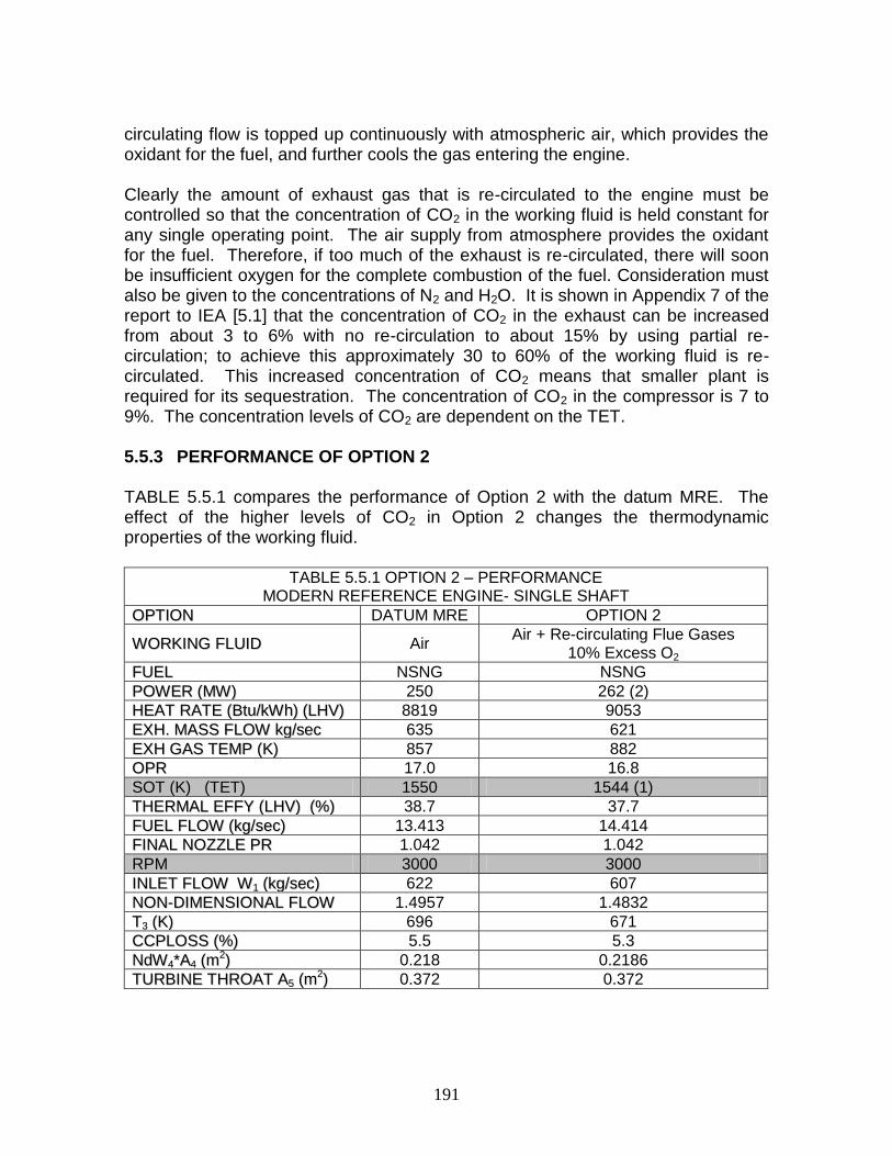
191
circulating flow is topped up continuously with atmospheric air, which provides the oxidant for the fuel, and further cools the gas entering the engine. Clearly the amount of exhaust gas that is re-circulated to the engine must be controlled so that the concentration of CO2 in the working fluid is held constant for any single operating point. The air supply from atmosphere provides the oxidant for the fuel. Therefore, if too much of the exhaust is re-circulated, there will soon be insufficient oxygen for the complete combustion of the fuel. Consideration must also be given to the concentrations of N2 and H2O. It is shown in Appendix 7 of the report to IEA [5.1] that the concentration of CO2 in the exhaust can be increased from about 3 to 6% with no re-circulation to about 15% by using partial re-circulation; to achieve this approximately 30 to 60% of the working fluid is re-circulated. This increased concentration of CO2 means that smaller plant is required for its sequestration. The concentration of CO2 in the compressor is 7 to 9%. The concentration levels of CO2 are dependent on the TET. 5.5.3 PERFORMANCE OF OPTION 2 TABLE 5.5.1 compares the performance of Option 2 with the datum MRE. The effect of the higher levels of CO2 in Option 2 changes the thermodynamic properties of the working fluid.
TABLE 5.5.1 OPTION 2 – PERFORMANCE MODERN REFERENCE ENGINE- SINGLE SHAFT
OOPPTTIIOONN DATUM MRE OPTION 2
WWOORRKKIINNGG FFLLUUIIDD Air Air + Re-circulating Flue Gases
10% Excess O2
FFUUEELL NSNG NSNG
PPOOWWEERR ((MMWW)) 250 262 (2)
HHEEAATT RRAATTEE ((BBttuu//kkWWhh)) ((LLHHVV)) 8819 9053
EEXXHH.. MMAASSSS FFLLOOWW kkgg//sseecc 635 621
EEXXHH GGAASS TTEEMMPP ((KK)) 857 882
OOPPRR 17.0 16.8
SSOOTT ((KK)) ((TTEETT)) 1550 1544 (1)
TTHHEERRMMAALL EEFFFFYY ((LLHHVV)) ((%%)) 38.7 37.7
FFUUEELL FFLLOOWW ((kkgg//sseecc)) 13.413 14.414
FFIINNAALL NNOOZZZZLLEE PPRR 1.042 1.042
RRPPMM 3000 3000
IINNLLEETT FFLLOOWW WW11 ((kkgg//sseecc)) 622 607
NNOONN--DDIIMMEENNSSIIOONNAALL FFLLOOWW 1.4957 1.4832
TT33 ((KK)) 696 671
CCCCPPLLOOSSSS ((%%)) 5.5 5.3
NNddWW44**AA44 ((mm22)) 0.218 0.2186
TTUURRBBIINNEE TTHHRROOAATT AA55 ((mm22)) 0.372 0.372

192
Notes on TABLE 5.5.1 (1) The SOT (TET) is 6K lower for Option 2 because the cooling flow of the HP turbine now contains about 7-9% CO2. This results in a small loss of cooling performance and so the SOT (TET) is reduced to retain blade metal temperatures. This is discussed in more detail later in connection with Option 3. (2) There is a small increase in power (4%) relative to the datum MRE but a slight reduction in thermal efficiency (one percentage point). The compressor true non-dimensional flow and its pressure ratio are virtually unchanged at synchronous rotational speed. 5.5.4 PHYSICAL MODIFICATIONS FOR OPTION 2
As can be seen from the performance details in Table 5.5.1 above, there would need to be only minimal changes to operate the datum MRE in a semi-closed cycle. However, if the plant were to be operated at an elevated pressure level throughout to increase power output, the engine casings and some other components would need strengthening. In summary, for Option 2 the changes to the engine are as follows.
Turbo-machinery – essentially unchanged. Combustor – changes are needed particularly if it is of the pre-mix type, to
accommodate the injection of the oxidant. Control system – changes would be needed to software logic to
accommodate variations in the re-circulation fraction in the semi-closed cycle. Additional control systems would be needed to control the valves and equipment for adjusting the re-circulation fraction. A new control system would be needed for the oxidant. A cooler is required to reduce the temperature of the re-circulated exhaust gases; this also would need a control system to regulate the amount of cooling. 5.5.5 DESCRIPTION OF OPTION 3 This is a closed cycle configuration in which the exhaust flow, which is virtually pure CO2, is re-circulated back to the inlet of the gas turbine (FIG 5.5.2). The fuel is natural gas. Oxygen is injected into the combustor to oxidise the fuel. More than the exact stoichiometric amount of oxygen (+10%?) would need to be injected in practice to ensure complete burning of the fuel and avoid unburned hydrocarbon emissions.

193
FIG.5.5.2 OPTION 3 - CLOSED CYCLE: CO2 WORKING FLUID: NATURAL GAS FUEL
A small amount of the exhaust is removed continuously for controlled disposal of the CO2 and to maintain a constant proportion of water in the exhaust. The exhaust must be cooled before it is returned to the engine. The above figure shows the engine in a combined cycle configuration, but the performance and description apply only to the engine itself (“simple cycle”). However, the diagram does serve to emphasize that because the working fluid is now essentially all CO2, the hot side of the HRSG boiler will need changing because of the different heat transfer properties of CO2 relative to vitiated air.
Removal of Excess CO2
HRSG
Compressor Turbine
Generator
Combustor
Generator
Pump
Condenser
Steam Turbine
Fuel (CH4) Oxygen
Water Separator
CO2 + H2O
Cooler H2O
Condenser

194
5.5.6 PERFORMANCE OF OPTION 3
TABLE 5.5.2 OPTION 3 PERFORMANCE
MODERN REFERENCE ENGINE – SINGLE SHAFT
OPTION DATUM
MRE
3 MODIFIED
COMPRESSOR
3 NEW
COMPRESSOR
WWOORRKKIINNGG FFLLUUIIDD AIR CO2 CO2
FFUUEELL NS NATURAL
GAS STOICHIOMETRIC
MIX NSNG / O2 STOICHIOMETRIC
MIX NSNG / O2
PPOOWWEERR ((MMWW)) 250 (1) 509 (1) 312 (1)
HHEEAATT RRAATTEE ((BBttuu//kkWWhh))
((LLHHVV)) 8819 9330 10075
EEXXHH.. MMAASSSS FFLLOOWW kkgg//sseecc 635 1188 758
EEXXHH.. GGAASS TTEEMMPP ((KK)) 857 954 1002
OOPPRR 17.0 26.7 17.0
SSOOTT ((KK)) ((TTEETT)) 1550 1510 (2) 1510 (2)
TTHHEERRMMAALL EEFFFFYY ((LLHHVV))
((%%)) 38.7 36.6 (3) 33.9 (3)
FFUUEELL FFLLOOWW ((kkgg//sseecc)) 13.413 139.69 (3) 92.61 (3)
FFIINNAALL NNOOZZZZLLEE PPRR 1.042 1.117 1.049
RPM 3000 3000 3000
NNOONN DDIIMM’’LL SSPPEEEEDD 8.80 11.31 11.31
IINNLLEETT FFLLOOWW,, WW11 ((kkgg//sseecc)) 622 1049 665
NNOONN DDIIMM’’LL FFLLOOWW 1.4957 2.124 1.347
TT33 ((KK)) 696 589 541
CCCCPPLLOOSSSS ((%%)) 5.5 3.5 3.2
ttppoollyy ((%%)) 91.0 92.7 93.4
NNddWW44**AA44 ((mm22)) 0.218 0.221 0.221
TTUURRBBIINNEE TTHHRROOAATT AA55((mm22)) 0.372 0.372 0.372
P4 / P6 15.41 23.06 15.68
NNOOZZZZLLEE AARREEAA ((AA88 ((mm22)) 10.83 10.83 10.83
(1) The power to produce the fuel and oxidant are not included (2) The SOT (TET) is reduced by 40K to maintain the same blade metal temperature as the datum MRE (3) Includes oxidant flow The table above shows two columns for Option 3. The first assumes that the compressor of the existing air breathing engine can be operated at the synchronous speed of 3000 rpm. To do this with the working fluid changed to CO2 would require a huge non-dimensional over-speed, and a large increase in pressure ratio; put another way the non-dimensional flow would increase considerably. The reason is the change in gas properties from air to CO2. The physical reason for this effect is discussed below. However, if the compressor could be modified to pass this flow and the casings of the engine strengthened to

195
accept the 50% increase in pressure, then the power would more than double relative to the datum engine. The last column is the more practical development of Option 3, but its performance in simple cycle is not as good (although its higher exhaust temperature means that it is more competitive in combined cycle configuration). A completely new compressor is required, giving the same pressure ratio as the datum MRE; however, strengthening of casings is not needed. The correct amount of H2O must be extracted from the exhaust. An exercise was completed to examine the effects of changing the H2O content of the re-circulating flow; it was found that the effects on performance are small – details are in [5.1]. 5.5.7 OPERATING SOT (TET) OF OPTION 3 Both versions of Option 3 would need a reduction in operating SOT (TET) of about 40K to maintain the datum MRE blade metal temperature in the turbine. The proof of this is given in Appendix 6 of the report to the IEA [5.1]. This research was suggested and instructed by the author and the detailed calculation was performed by Mr. Whellens (MSc student, Cranfield University). In summary, the following procedure was used. The length of the blade cooling passages and also the blade chord and span were kept constant. The mainstream and cooling fluid temperatures and pressures were obtained from the performance results. The cooling fluid flow rate was 5% of the mainstream flow rate. Mainstream flow speed was assumed to be Mach 1; this is a simplification but allows reasonable comparison between the two cases. Cooling passage flow speed was assumed to be 0.3 Mach; in practice this would require a small change in the diameter of the cooling passages. Heat transfer coefficients were then calculated from the fluid properties and the empirical relationship: Nu = 0.023 Re0.8 Pr0.4 This resulted in the following ratios of heat transfer coefficients:- (hg/hc)air = 1.82 (hg/hc)CO2 = 2.0 hg and hc are the mainstream and coolant heat transfer coefficients respectively.
This allowed the blade metal temperatures to be calculated.

196
5.5.8 PHYSICAL MODIFICATIONS FOR OPTION 3 Unlike Option 2, the change of working fluid causes, in this case, very large changes to the matching of the engine. The main effect is that a gross (and impossible) increase in aerodynamic over-speed would be required in the compressor to retain synchronous operation. What this means in simple terms is that if an attempt were made to drive the engine to its normal synchronous speed of 3000 or 3600 rpm, the compressor inlet flow would generally choke long before this speed was reached, causing engine surge. The gas property changes are discussed above (Section 5.3.3). A demonstration of the matching changes for Option 3 is shown in Appendix 12 (wholly researched and written by the author) covering a typical compressor, combustor, turbine and whole engine. As a measure of the effect, it is worth noting that CO2 is about 50% more dense than air at a given pressure and temperature, and the speed of sound in CO2 is about 79% of the speed of sound in air at a given temperature. It can be safely assumed that no existing compressors are capable of the amount of aerodynamic over-speeding expected to achieve the first column of TABLE 5.5.2. Thus, an existing engine would need a new compressor to operate with CO2 as the working fluid, if the rest of the engine were retained. Any new compressor designed for operation on CO2 could use existing technology and would operate satisfactorily. If the combustor size were unaltered, it would exhibit a lower pressure drop with CO2 because the Mach number levels would be lower. If the pressure drop were say 5.5% with air, it would be about 3.7% with CO2, giving a small performance benefit (1.0% in power and 1.0% of heat rate). In practice, the combustor would have to be re-designed to give the pressure drop required to drive the cooling of the combustor and the first row of turbine NGVs. If, when changing to CO2, the turbine were unaltered, and operated synchronously, it would effectively have a lower loading than when operating on air due to its higher effective speed. This would result in a small efficiency gain, of the order 2% in the MRE engine under consideration (worth about 3.2% power and 3.2% heat rate). The logic for this is more fully explained in Appendix 12.
An alternate way of overcoming the compressor speed problem is to insert a gearbox between the turbine and the compressor. This would involve mechanical complication but in some circumstance may be an easier development option than to modify the compressor.
In summary, the following changes would be needed for Option 3.

197
Turbo-machinery – a new compressor is essential. An existing turbine system could probably be used, but it will operate at a higher expansion ratio and should be checked on a case by case basis.
Combustor – this would need substantial modification. Control system – this would need modification and additions in order to cope
with the oxidant and the closed circuit characteristics. 5.5.9 A NOTE ON FREE POWER TURBINES The effects of using a free power turbine in synchronous operations have been explored by the author subsequently to the publication of the report to the IEA [5.1]. The results are reported in the paper [5.3], which is included in the thesis as Attachment 4. The reader is referred to Fig 3 and Tables 3 and 5 of this reference. In summary the effects are as follows. For the datum natural gas fuelled MRE there is of course no change in the engine performance from fitting a free power turbine instead of using a connected shaft. For the hydrogen-rich fuelled Options 1A and 1B, there is a slight increase in power with a free power turbine because the compressor operates at a slightly higher speed, flow and pressure ratio to maintain the correct capacity of the MRE free power turbine nozzle guide vanes. For the partially closed loop case, Option 2, there is a substantial increase in flow, pressure ratio and compressor speed to retain the MRE free power turbine nozzle area unchanged. The compressor, which is assumed to be based on the datum MRE compressor, requires a double “0” stage. There is also a problem with tip speeds and flow areas at the rear of the power turbine. For the closed loop case, Option 3, the compressor is new anyway and so is not affected when a free power turbine is used. So the performance is essentially identical to the connected shaft configuration. Table 5 in [5.3] shows that unchanged flow, power and thermal efficiency can be achieved; however, the flow capacity of the free power turbine must be reduced by 25% relative the datum MRE. In conclusion, each case must be explored separately. There is no over-riding performance reason to choose the datum MRE engine as either a free power turbine or a connected shaft configuration.

198
5.6 CONCLUSIONS – INDUSTRIAL NOVEL CYCLES Specific novel industrial engine configurations (called “Options”) have been examined at the request of the International Energy Agency (IEA). They were all aimed at achieving zero output of CO2 emissions. They are summarised in TABLE 5.6.1 below. Options 1A and 1B are simple gas turbines but use hydrogen rich fuels. Option 2, also a simple gas turbine, uses natural gas fuel but is incorporated in a partially closed loop, so its working fluid is CO2 rich, which assists sequestration of the CO2. Option 3 is also a single shaft gas turbine using natural gas fuel; however, it is incorporated in a wholly closed loop and its working fluid is CO2. An oxidant such as oxygen is injected into the combustor to react with the fuel. The IEA wished to know how much the design of the Options differed from a standard industrial gas turbine. Therefore, an engine was “invented” as a datum, called the “Modern Reference Engine” (MRE). The MRE has modern levels of cycle parameters and component efficiencies and is sized at 250MW. Its overall pressure ratio is 17 and its turbine entry temperature is 1550K. Its fuel is natural gas. The MRE configuration that has been used as datum has a single shaft connected directly to a synchronous electrical load. If a free power turbine had been chosen, performance results for the hydrogen rich fuels (Options 1A and 1B) would have been slightly different but the degree of change to the datum engine (a free power turbine version of the MRE) would have been similar to the connected shaft case. For Option 2 (partially closed loop), there are significantly more changes in the free power version, mainly in the compressor, and significant performance issues. For Option 3, major changes are required as for the connected shaft version. The free power turbine versions are discussed in Section 5.5.9. There is no over-riding reason to choose a free power turbine configuration rather than a connected shaft configuration for any of the Options. TABLE 5.6.1 shows a summary of the main parameters, the overall performance and the degree of change for the connected shaft, synchronous versions of all the Options. The main technology challenges for all the Options are the combustor and the control system, which are essentially totally new in each case. The combustor will be a particular challenge for the hydrogen fuelled Options 1A and 1B if, to reduce NOx, they employ pre-mix lean burn combustor technology, because of the high flame speed of hydrogen compared with natural gas.

199
For the Option 3 (in closed loop, with CO2 working fluid), major changes are needed to the compressor relative to the datum MRE, because of the change in working fluid properties. Please see TABLE 5.6.1 below and its footnotes.
TABLE 5.6.1 COMPARISON OF NOVEL CYCLES – CONNECTED SHAFT RESULTS
OPTION DATUM Modern
Reference Engine (MRE)
1A MRE with hydrogen rich fuel
1B MRE with H2/N2 fuel
mix (Note 1)
2 MRE in partially
closed loop
3 MRE in closed loop with CO2 working fluid a) “Modded” compr. b) New compr. (4)
FUEL NS Nat
gas 95/5 molar
H2/N2 50/50 molar
H2/N2 NSNG NSNG
WORKING FLUID
AIR AIR AIR AIR + CO2 CO2
PLANT CYCLE
OPEN OPEN OPEN PART
CLOSED CLOSED
OVERALL PRESSURE RATIO
17.0 17.1 19.2
[16.5] 16.8
a) 26.7 b) 17.0
SOT K (TET) 1550 1550 1550 1544 (3) a) 1510 (3) b) 1510 (3)
INLET FLOW kg/s
622 622 620 [622]
607 a) 1049 b) 665
POWER MW 250 261 336
(Note 2) [225]
262 a) 509 b) 312
THERMAL EFFICIENCY %
38.7 39.6 43.6(Note
2) [37.2]
37.7 a) 36.6 b) 33.9
EXHAUST TEMP. K
857 852 835 [857]
882 a) 954
b) 1002
COMPRESS-OR
DATUM NO
CHANGE SMALL
UPGRADE NO
CHANGE a) MODIFIED b) NEW
COMBUSTOR – DIFFUSION
DATUM NEW
INJECT-ORS
NEW INJECT-
ORS
NEW INJECT-
ORS
a) NEW b) NEW
COMBUSTOR – PRE-MIX
DATUM MAJOR
CHANGE SOME
CHANGE SOME
SHANGE a) NEW b) NEW
TURBINES DATUM NO
CHANGE THROAT CHANGE
NO CHANGE
a) UPGRADE? b) UPGRADE?
FUEL AND CONTROLS
DATUM NEW NEW MUCH
CHANGE a) MODIFIED b) MODIFIED
% of ENGINE CHANGED
DATUM 20 – 40% ABOUT
25% 20 – 40%
a) 50 – 75% b) 50 – 75%
Please see notes below

200
(1) Alternative figures shown thus [..] for Option 1B take account of the power required to compress the nitrogen into the engine. (2) Large input of nitrogen is “free”. (3) TET reduced from 1550K to maintain datum turbine metal temperatures. (4) The power to produce the fuel is not accounted. Interpolation between options 1A and 1B may be made on a linear basis to a good approximation.

201
CHAPTER 6
OVERALL CONCLUSIONS AND FUTURE WORK
6.1 CONCLUSIONS The objectives of this thesis are twofold; the first objective has been to explore potential improvements in the design of aero and industrial gas turbines aimed at reducing or eliminating their emissions of CO2; the second objective is to find ways of reducing the noise of aero gas turbines and to link this with the potential performance improvements. Initial background studies on gas turbine technology history, on climate change and on aircraft noise have been presented (Chapter 2). Three separate but related studies have then been completed as follows. Aero engine optimisation (Chapter 3) Hydrogen fuelled aero engines (Chapter 4) Industrial novel cycles (Chapter 5) 6.1.1 ENGINE TECHNOLOGY Gas turbine engines were invented in the 1920s and after many travails first entered service as propulsion for fighter aircraft late in WW2. They have subsequently developed rapidly and are now the preferred propulsion means for most transport and military aircraft, and are used in ground-based plants for power generation and in ships for propulsion. The earliest engines were single shaft turbojets (bypass ratio zero) with centrifugal compressors; overall pressure ratio was about 4, combustor outlet temperatures about 900K and take-off thrust around 4kN. Modern engines are turbofans with two or three shafts and axial compressors; bypass ratio values are 6 to 9, overall pressure ratios are over 40, combustor outlet temperatures are over 1800K and take-off thrusts reach over 450kN. Cruise specific fuel consumption is presently about half that of the civil transport engines of the 1950s. Thermal efficiencies of industrial engines are about twice the values of the original machines. Noise levels of aero gas turbines are of the order 20PNdB lower than the early jet engines. Technology advances are still eagerly sought and the flow of improvements shows no signs of abating. The technology advances explored in this thesis are no doubt also under constant scrutiny in industry, but results are unlikely to be published due to commercial sensitivity.

202
6.1.2 CLIMATE CHANGE Data from the Met Office is presented showing that global warming is taking place; average atmospheric temperatures have increased by about 0.8C over the past 100 years. Also, evidence from air bubbles trapped in the ice and recent air measurements show that atmospheric concentration of CO2 is higher now than at any time in the past 400,000 years; the concentration remained stable until about a century ago but has since risen about 30% (290 to 380 ppm). The contribution of aviation to “greenhouse gases”, including CO2, NOx and H2O is reported variously between 2% and 13% of man-made emissions. However, it is likely that aviation’s contribution to man-made emissions of CO2 alone is around 3.5%. 6.1.3 NOISE Gas turbine jet noise was recognised as a problem as early as 1940. In the 1950s, turbojet and low bypass ratio turbofans were powering the earliest civil airliners to satisfy the demand for high speed travel. They were noisy mainly due to jet noise from to their high jet velocities and partly due to tones produced by LP compressor blade wakes interacting with downstream blade rows. By the 1960s, a strong public anti-noise lobby had developed, which still exists. So engine designers made strenuous efforts to reduce jet noise. The big breakthrough came in the late 1960s with the arrival of the high bypass ratio turbofans, with their much lower jet velocities and their single stage fans with high spacing to the stators and no IGVs. Subsequently, with more increases in bypass ratio, which further reduced jet noise, fan noise became the main problem and that is the current position. Fan, or propeller, noise is a major deterrent to the advancement of open rotor (propfan) developments. 6.1.4 AERO ENGINE OPTIMISATION A study of potential improvements to aero gas turbines for transport aircraft has been presented. The improvements focus on choice of bypass ratio and installation configurations although all other possible methods - overall pressure ratio, combustor outlet temperatures and efficiency changes - are explored. Relationships between specific fuel consumption and noise are presented for a large range of bypass ratios for long cowls, short cowls and open rotors. It is shown that by increasing the choice of cowled turbofan design bypass ratio above a datum value of 6, there are potential benefits in aircraft fuel burn, DOC and noise, despite the associated increases in engine weight. These results are summarised on FIG 3.7.1. It can be seen that apparently the best choice of cowled engine for fuel burn and DOC is a bypass ratio around 12 to 15, with a short cowl installation. Useful gains of 6% in fuel burn and 3% in DOC for a 5000nm mission look possible with short cowl configurations.

203
For all the cowled aero engine bypass ratios studied, forward fan noise is louder than rearward jet noise. Although fan forward noise at bypass ratio 12 to 15 is about 5dB less than at bypass ratio 6 it could be reduced further by more increase in bypass ratio. Open rotors (propfans) give better installed fuel consumption than the best short cowled engines, and this translates into potentially a further 7% reduction in fuel burn and a further 1% improvement in DOC despite the engine weight. However, the noise of open rotor configurations militates against them, relative to cowled engines. The issue of thrust reversing is acknowledged but not addressed. Short cowl engines have the option of a standard reverser or use of variable pitch fans. Open rotors would require variable pitch propellers. Increases in overall pressure ratio, combustor outlet temperature or efficiencies give potential gains in fuel burn and possibly DOC (depending on how much the engine cost increases). Increases in combustor outlet temperature would increase the optimum bypass ratio for fuel burn and DOC. 6.1.5 HYDROGEN FUELLED AERO ENGINES In Chapter 4, a study of hydrogen fuelled aero gas turbines has been presented, which is a summary of work done for the EU “Cryoplane“ research contract. It has two elements. In the first, the effects of fuelling “conventional” gas turbines with hydrogen is explored; in the second, some novel cycles are investigated which make use of the “cold sink” of the hydrogen (-253C) or its high pressure following pumping from the aircraft tanks. A performance model of the IAE V2527-A5 engine was created and used as the main datum for the assessments. It is shown that thermodynamically, there are small but useful benefits to “conventional” turbofans. This effect arises from the very high Cp of hydrogen. Gains in thrust at a combustor outlet temperature of up to 28% and reduction in energy specific fuel consumption of about 4.5% are shown. The main changes to turbofans designed to burn kerosene are in the fuel system and combustor. Some novel cycles for hydrogen fuelled aero gas turbines are explored to examine their potential for good fuel consumption. Potential benefits in performance arise because of the “cold sink” offered by the hydrogen fuel and the fact that the fuel, kept as a liquid in the aircraft tanks, can be pumped to high pressure with very small expenditure of power. Many novel possible configurations were considered, but only three were considered viable and attractive. The others either offered little gain or had practical difficulties in sealing the ancillary turbomachinery required.

204
The winners were: -
Cooling of the air entering the core via a fuel-cooled heat exchanger; this offered 4.4% better cruise specific fuel consumption and 6.7% more take-off thrust than the conventional engine with the same turbine entry temperature because a higher overall pressure ratio could be used for the same HP turbine loading and because the extra power available at the LP turbine allows the bypass ratio to be increased slightly. Cooling of the air used to cool the HP turbine; this gave 1.5% better specific fuel consumption and 28.1% more take-off thrust because the turbine entry temperature could be raised by 141K at the same turbine life, so the bypass ratio could be increased from 4.8 to 6.5. Pre-heating and evaporating the fuel using the engine core exhaust heat; this gave 2.6% better specific fuel consumption and a 1% loss in take-off thrust with turbine entry temperature and overall pressure ratio unchanged from the datum.
6.1.6 INDUSTRIAL NOVEL CYCLES Studies are presented in Chapter 5 that are a summary of the author’s work on a contract placed on Cranfield University by the IEA. The objectives were to explore specified “Options” to modify standard industrial gas turbines to eliminate their emissions of CO2. The first “Option” was to use carbon-free fuels, namely mixtures of hydrogen and nitrogen. The second was to place a natural-gas fuelled gas turbine in a partially closed loop so that the working fluid was rich in CO2: this meant that the exhaust could be processed to extract the CO2 using much smaller plant than that required to process the exhaust of an open loop configuration. The third was to place the natural gas fuelled gas turbine in a closed loop plant with CO2 as the working fluid thus making sequestering of the CO2 possible with the smallest possible extra plant. A performance model of a fictitious modern single shaft industrial engine (the “MRE”) was made as the basis of the studies. A new gas turbine performance code was written (“Variflow”) capable of using any species of gas as working fluid or fuel. The “Options” specified by the IEA were modelled and detailed conclusions are drawn in Chapter 5 and are summarised below. In the case where the fuel is essentially hydrogen with a minimal amount of nitrogen mixed in, the changes to a standard gas turbine are confined to the combustor and the fuel system. There is a slight performance gain.

205
If the fuel is hydrogen with a high proportion of nitrogen mixed in, it is likely that the turbine throat area will need enlarging to accommodate the nitrogen that arrives with the fuel. Other changes are again the combustor and fuel system. There are considerable increases in power of the gas turbine alone, but account needs to be taken of the power required to compress the fuel mixture. In the case of the partially closed loop, fuelled by natural gas, a small upgrade of the compressor is required because of the extra content of CO2 in the working fluid. Combustor and fuel system changes are needed. There is a small power gain but a slight loss in thermal efficiency. Finally, for the closed loop case, where the working fluid is entirely CO2, the turbine can be preserved by making radical changes to the compressor. Combustor and fuel system changes are need again, including a new system to inject the oxidant for the fuel. Depending on the changes made there can be significant gains in power, but not much change in thermal efficiency. 6.1.7 OVERALL CONCLUSION The objectives of the thesis have been achieved. Relative to present day gas turbines, gains in aero engine and industrial engine performance are possible; reductions in aero engine noise are also possible. Such improvements are available with present day technologies. They would reduce the environmental impact of gas turbines. The optimum aero engine bypass ratio is shown to be about 12 to 15; this compares with 5 to 6 shown in the 1975 attachment 1. For the future, it can be confidently predicted that further performance improvements will be achieved for all applications of gas turbines. 6.2 FUTURE WORK 6.2.1 NOISE ESTIMATION CODES The noise estimation code available to the author via Cranfield University is based on jet noise correlations that have a good parentage (RR and Boeing for example). However, the code would benefit from further work to refine the accuracy of jet noise results. However, in its present form, the code gives useable comparisons for jet noise. However, the code needs substantial effort to improve calculation of the attenuation from duct linings in the intake and jet pipes. It attempts to use an ESDU method but the results are not always consistent with expectations from other sources, and the code does not operate reliably. Since fan noise is likely to dominate other sources in gas turbines for some time to come, intake and bypass duct lining noise attenuation is crucial.

206
The author has not used the methods offered by this code on turbine and combustor noise. Other codes and methods could be investigated with possible benefits; Smith [2.20] gives a comprehensive list covering pre-1989 methods. 6.2.2 WEIGHT ESTIMATION METHODS Weight estimation of gas turbines at an early stage in their design is problematic. The author explored various possible methods but most of them were based on correlations of current engines in such a way that their results were somewhat questionable at very high bypass ratios. Only the method by Sagerser et al [3.59] seemed scientifically sound enough to use over the full range of bypass ratios considered herein. Unfortunately, the method was developed for VTOL engines; consequently when used on propulsion engines it gives weight estimates of known engines that are lighter than the published values. The method is nevertheless sound; so if the correlations were updated to include high pressure ratio modern propulsion engines, it could form a useful basis for preliminary estimates of engine weight. A pressure level term is required for the core components Another weight estimating method found by the author is one published in recent years by Glenn Research Centre called EngSim [3.62]. This has not been examined because it appeared to be an educational tool; however, it may be worth study. 6.2.3 TURBOMATCH PERFORMANCE CODE – FAN SIMULATION The gas turbine performance code in standard use at Cranfield University is called “Turbomatch”. It has been developed for many years. In spite of its considerable capabilities, lack of resource has caused it to fall behind the times in certain aspects. The aspect that prevented the author from using it for this thesis was that it does not allow the use of different pressure ratios at the outer and inner portions of the fan. This is particularly significant at high bypass ratios, and so the need to add this capability will become increasingly urgent. The code is presently being updated to include simulation of propellers and propfans. It is also being made able to simulate transient (non steady state) performance. Both these facilities are needed to bring the code up to modern standards. End of text

207
CHAPTER 7.0 REFERENCES BACKGROUND (CHAPTER 2) [2.1] Whittle, Sir Frank. “Jet; the Story of a Pioneer”. Frederick Muller Ltd., 1953. [2.2] http//en.wikipedia.org/wiki/General_Electric_CF6 accessed 13th August 2008. [2.3] Lighthill M. J. “On Sound Generated Aerodynamically. I. General Theory”. Proc. R. Soc. London. A 211; pages 564-587. 1952. [2.4] Jackson A. J. B. “Some Future Trends in Aero Engine Design for Subsonic Transport Aircraft”. Transactions of ASME; Journal of Engineering for Power; Pages 281 to 289. April 1976. Proceedings Paper ASME 75-GT-2, 1975. [2.5] Cohen H., Rogers G. F. C. and Saravanamuttoo H. I. H. “Gas Turbine Theory”. 4th Edition. Longmans. 1998. ISBN 0-582-23632-0. [2.6] Walsh P. P. and Fletcher P. “Gas Turbine Performance”. Book; Blackwell Science. ISBN 0-632-04874-3. 2001 [2.7] Tyndall Centre for Climate Change Research. “Decarbonising the UK (September 2005) – Contribution of UK Aviation to Climate Change” updated December 2007 [2.8] Smith P. F. “Beware the Sands of Time”. Lecture to the Cambridge Society, Derbyshire Branch, Hassop Hall, 10th November 2008. [2.9] Met Office Hadley Centre “Climate Change – the Big Picture; Climate Change Facts”. www.metoffice.gov.uk/index.html accessed 13th August 2008 [2.10] IPPC “Climate Change 2007: The Physical Science Basis. Summary for Policymakers”. Published by the Intergovernmental Panel on Climate Change, 2007. [2.11] BBC News: “Science and Nature”. Broadcast 20th August 2007 [2.12] Green J. E. “Greener by Design – the Technology Challenge”. The Royal Aeronautical Journal, Pages 57 to 113, February 2002.

208
[2.13] Lowe J. (Chairman) et al. “Air Travel – Greener by Design”. Published under the auspices of the R. Ae. S., SBAC, BATA and the Department of Trade and Industry, et al. Sept 2003. [2.14] I.Mech.E. “Novel Propulsion Systems for the 21st Century”. I.Mech.E. Conference, Bristol, 20th November 2007 [2.15] Morley A. W. “Estimation of Aeroplane Noise Level: Some Empirical Laws with an Account of the Present Experiments on which they are Based”. Aircraft Engineering 11 (123), 1939; pp187-189. [2.16] Rolls-Royce “The Jet Engine” published 2005. ISBN 0902 121 235 [2.17] North East Aircraft Museum http://neam.co.uk/comet.html accessed 14th August 2008 [2.18] Salford University. “Aircraft Noise”. Published course notes from: - http://www.acoustics.salford.ac.uk/studentt _area /bsc2 accessed 18th September 2008. [2.19] Envia E., Thomas R. Presentation by NASA Acoustics Discipline Team, 2007. www.grc.nasa.gov/WWW/Acoustics/pdfs/HQ_Presentation_10167 [2.20] Smith M. J. T. “Aircraft Noise”. Book; Cambridge University Press; 1989 hardback ISBN 0 521 331862: 1994 paperback ISBN 0 521 616999. [2.21] Dowling A., Hynes T. “Towards a Silent Aircraft” Lecture to the Derby Branch of the Royal Aeronautical Society 10th September 2008 AERO ENGINE OPTIMISATION (CHAPTER 3) [3.1] www.rolls-royce.com.civil_aerospace/products/airlines/trent800, January 2008 [3.2] Aerospace International. April 2008 [3.3] The Aerospace Professional April 2008 [3.4] GE-Aviation Innovation.htm [3.5] Denton J. D. and Xu L. “The effects of Lean and Sweep on Transonic Fan Performance”. ASME GT-2002-30327, Amsterdam, June 3-6 2002

209
[3.6] Bergner J., Kablitz S. and Hennecke D. K. “Influence of Sweep on the 3D Shock Structure in and Axial Transonic Compressor”. ASME GT-2005-68835, Reno-Tahoe June 6-9, 2005 [3.7] He L. and Ismael J. O. “Computations of Bladerow Stall Inception in Transonic Flows”. J. R.Ae.S. Vol 103, Number 1025 July1999 [3.8] Kurzke J. “GasTurb” Gas Turbine Performance Code. http://www.gasturb.de 2008. [3.9] Jane‟s Aero-Engines. Various issues including Issue 21 – 2007. jae.janes.com [3.10] Jackson A. J. B. “A Short Course on Gas Turbine Performance”. Lecture Notes first published 1973 and delivered at Derby College of Art and Technology and subsequently annually to Rolls-Royce plc. [3.11] Ghenaiet A. “Analyses and Optimisation of a Propulsion Cycle for Unmixed High Bypass Turbofan”. ASME GT-2008-50340. 2008 [3.12] Cumpsty N. “Jet Propulsion”. Cambridge University Press. 1997. ISBN 0-
521-59330. [3.13] Jenkinson L. R., Simpkin P. and Rhoder D. “Civil Jet Aircraft Design” published in1999 by Arnold; ISBN 0340 74152X [3.14] Smith S. F. “A Simple Correlation of Turbine Efficiency”; Journal of the R. Ae. S. 69 (1965), p 467. [3.15] Ramsden K. W. “Axial Turbine Lecture Notes”. Cranfield University School of Engineering, 2007 [3.16] Laskaridis, P. Private communication 2008. [3.17] Jackson A. J. B. “Aero Gas Turbine Windmilling, Relighting and Pull-Away: a Position Paper”. Rolls-Royce University Technology Centre in Performance Engineering at Cranfield University. 20th November, 1998. [3.18] Zimbrick R. A. and Colehour J. L. “An Investigation of Very High Bypass Ratio Engines for Subsonic Transports”. AIAA Propulsion Specialist Conference, Boston 1988. Paper No. 88-2935 [3.19] Daggett D. L., Brown S. T. and Kawai R. T. “Ultra-Efficient Engine Diameter Study”. NASA/CR-2003-212309. 2003.

210
[3.20] Hall C. A., Crichton D. “Engine Design Studies for a Silent Aircraft”. Journal of Turbomachinery Vol129, July 2007, pages 479-487 [3.21] Bodony D. J. “The Prediction and Understanding of Jet Noise”. Center for Turbulence Research - Annual Research Briefs 2005 Page 367. [3.22] Westley R., Lilley G. M. “An Investigation of the Noise Field from a Small Jet and Methods for its Reduction”. Tech. Rep.53, College of Aeronautics, Cranfield, England, UK.1952 [3.23] Lassiter L. W., Hubbard H. H. “Experimental Studies of Noise from Subsonic Jets in Still Air” NACA TN-2757; 1952 [3.24] Lighthill M. J. “On Sound Generated Aerodynamically. II. Turbulence as a Source of Sound”. Proc. R. Soc. London. 1954. A 222; pages 1-32. [3.25] Lassiter L. W., Hubbard H. H. “The Near Field Noise of Static Jets and Some Model Studies of Devices for Noise Reduction” NACA Report 1261; 1956 [3.26] Olsen W., and Friedman R. “Jet Noise from Co-Axial Nozzles over a Wide Range of Geometric and Flow Parameters” NASA TM X-71503 Lewis Research Centre, Cleveland, Ohio. AIAA 12th Aerospace Sciences Meeting; 30th January – 1st February 1974 [3.27] Fisher M. J., Preston G. A. and Bryce W. D. “A Modelling of the Noise from Simple Coaxial Jets, Part 1; With Unheated Primary Flow”. Journal of Sound and Vibration (1998) 209(3), 385-403 [3.28] Bhat T. R. S. and Blackner A. M. “Installed Jet Noise Prediction Model for Coaxial Jets”. AIAA 98-0079 [3.29] Hubbard H. H. (Editor). “Aeroacoustics of Flight Vehicles: Theory and Practice. Vol. 1; Noise Sources”. NASA Reference Publication 1258, Vol. 1 WRDC Technical Report 90-3052. 1991. [3.30] Russell J. W. “An Empirical Method for Predicting the mixing Noise Levels of Subsonic Circular and Coaxial Jets”. NASA CR-3786 February 1984 [3.31] Di Fiore dos Santos, G., Barbosa J. R. and Pilidis P. “Analysis of Turbofan Empirical Noise Prediction Methods”. AIAA 2005-3076 11th AIAA/CEAS Aeroacoustics Conference 23-25 May 2005, Monterey, California. [3.32] Pilon A. R. and Morris P. J. “A Semi-analytical Method for Jet Noise Prediction”. AIAA 99-0076. 1999.

211
[3.33] Lighthill M. J. “Jet Noise”. AGARD Report 448 April 1963 [3.34] Heron N. and Lemaire S. “Coaxial Jet Noise Predictions from Statistical and Stochastic Source Models”. AIAA 2001-2205. 2001. [3.35] Stone J. R., Zola C. L. and Clark B. J. “An Improved Model for Conventional and Inverted-Velocity-Profile Coannular Jet Noise”. AIAA-99-0078, 1999. [3.36] Bhat T. R. S. and Seiner J. M. “The Effect of Velocity Profiles on Supersonic Jet Noise”. AIAA 93-4410, 1993. [3.37] Janarden B. A., Hoff G. E., Barter J. W., Martens S., Gliebe P. R., Mengle V., Dalton W. L. “AST Critical Propulsion and Noise Reduction Technologies for Future Commercial Subsonic Engines. Separate-Flow Exhaust System Noise Reduction. Concept Evaluation”. NASA Report CR 2000-210039, 2000. [3.38] SAE. “Gas Turbine Jet Exhaust Noise Prediction”. SAE Report ARP 876-D, 1994. [3.39] SAE. “Gas Turbine Coaxial Exhaust Flow Noise Prediction”. SAE Report AIR 1905, 1985. [3.40] ESDU. “Aircraft Noise Series”. Item 98008 April 2000. [3.41] Heidelberg l. J. “Comparison of Tone Mode Measurements for a forward swept and Baseline Rotor Fan”. NASA/TM-2003-212378 and AIAA-2003-3293. 2003 [3.42] Flight International. “Rolls-Royce Trent 800”. Poster from “The Flight Collection, Quadrant Picture Library, The Quadrant, Sutton SM2 5AS. [3.43] Miller C. “Euler Analysis of a Swirl Recovery Vane Design for Use with an Advanced Single-rotation Propfan”. U.S. Government Printing Office, Washington DC. 1988. [3.44] Heidmann M. F. “Interim Prediction for Fan and Compressor Source Noise”. NASA TM X-71763, 1975. [3.55] http://silentaircraft.org/sax40.html accessed 21st September 2008 [3.56] Dickens A. “Highly Loaded Compressors” PhD Thesis Cambridge University 2008 [3.57] Gerend R. P. and Roundhill J. P. “Correlation of Gas Turbine Engine Weights and Dimensions”. AIAA 70-669, June 1970.

212
[3.58] Colmenares F. “Engine Nacelle Weight and Dimensions Report”. Cranfield University. School of Engineering, 2000 [3.59] Sagerser D. A., Lieblein S. and Krebs R. P. “Empirical Expressions for Estimating Length and Weight of Axial-Flow Components of VTOL Powerplants”. NASA TM X-2406 December 1971. [3.60] Pera R.J., Onat E., Klees G. W., and Tjonneland E. “A Method to Estimate Weight and Dimensions of Aircraft Gas Turbine Engines. Volume 1: Method of Analysis”. NASA CR 135170 May 1977. [3.61] Clavier J. “Aero Gas Turbine Engine Design Project (AVIC) Ultra High Bypass Ratio Study”. MSc Thesis.Cranfield University, 2008. [3.62] Glenn Research Centre “EngSim Beta Version 1.7A” http://www.grc.nasa.gov/WWW/K-12/airplane/engsim.html [3.63] http://www.boeing.com/commercial/777family/pf/pf_200product.html accessed 12th August 2008. [3.64] Foster A. Cranfield University Aerospace Group DOC code; 2008. [3.65] Hager R. D. and Vrabel, D. “Advanced Turboprop Project”. Washington D.C.: U.S. Government Printing Office, 1988. [3.66] Ciszek R. S. “Prop Fan Propulsion Concepts: Technology Review, Design Methodology, State-of-the-Art Designs and Future Outlook”. University of Virginia Department of Mechanical and Aerospace Engineering Senior Thesis Project, 25th March 2002. http://members.aol.com/sciszek/propfan.htm. [3.67] Lehouchou N. “Performance and Integration Assessment of a Counter Rotating Ducted Propfan”. Cranfield University MSc Thesis 2005. [3.68] Wikipedia http://en.wikipedia.org/wiki/Rolls-Royce_Dart 12th May 2008 [3.69] Vickers Viscount Network www.vickersviscount.net/ 12th May 2008 [3.70] Siuru W and Busick J. D. “The Next Generation of Aircraft Technology”, 2nd Edition 1994. TAB Books, McGraw-Hill; ISBN 0-8306-4376-1 (p). [3.71] GE-Aviation Innovation.htm. Accessed April 2008 [3.72] Wikipedia http://en.wikipedia.org/wiki/EPI_TP400 Accessed10th May 2008

213
[3.73] Bowles M. D. and Dawson V. P. “The Advanced Turboprop Project”. NASA. Written 1998, updated 2001. <http://history.nasa.gov/SP-4219/Contents.html> [3.74] Kuznetsov N. D. “Propfan Engines”. AIAA 93-1981. AIAA/ SAE/ ASME/ ASEE 29th Joint Propulsion Conference and Exhibit, 28-30 June 1993. [3.75] Rohrbach C. “A Report on the Aerodynamic Design and Wind Tunnel Test of a Prop-Fan Model” AIAA Paper 76-667 AIAA/SAE 12th Propulsion Conference Palo Alto 26-29 July 1976 [3.76] Stefco G. L., Jeracki R. J. “Wind-Tunnel Results of Advanced High-Speed Propellers at Take-off, Climb and Landing Mach Numbers”. NASA TM 87030. Written November 1985, general release February 1989 [3.77] Bartel H. W., Swift G. “Near-Field Acoustic Characteristics of a Single-Rotor Propfan”. AIAA-89-1055 AIAA Aeroacoustics Conference April 10-12 1989 [3.78] Gordon B. J. The Development of the Unducted Fan. 11th H. P. Folland Memorial Lecture 14th April, 1988; Aerospace magazine, July 1988, page 22. [3.79] Robinson T. “The Way Forward”. Article (page 20) in Aerospace International June 2008. [3.80] Taylor M. “Open Rotor Engine Design and Validation”. Presentation to Conference; “Greener by Design. Aviation and the Environment: Where are we Going?”. R.Ae.S. HQ, London; sponsored by Department for Business Enterprise and Regulatory Reform. 7th October, 2008. HYDROGEN FUELLED AERO ENGINES (CHAPTER 4) [4.1] Westenberger A. “Liquid Hydrogen Fuelled Aircraft – System Analysis”. (“Cryoplane”). Executive Publishable Summary. EU Project GRD1-1999-10014. 24th September 2003. [4.2] Brewer G. D. “Hydrogen Aircraft Technology”. CRC Press. ISBN 0-8493-5838-8 1991 [4.3] Silverstein A. and Hall E. W. “Liquid Hydrogen as a Jet Fuel for High Altitude Aircraft”. NACA RM E55C28a; National Advisory Committee for Aeronautics – Lewis Flight Propulsion Laboratory, Cleveland OH, 1955. [4.4] Robinson T. “Hail, SESAR” Aerospace International, page 24-25, March 2008 [4.5] http://en.wikipedia.org/wiki/Ariane-(rocket)

214
[4.6] Brewer G. D., Morris R. E., Lange R. H. and Moore J. W. “Study of the Application of Hydrogen Fuel to Long Range Subsonic Transport Aircraft”. NASA CR-132559, Lockheed-California Co and Lockheed-Georgia Co., Burbank, January 1976. [4.7] Jackson A. J. B. “The Effects of the Fuel Situation on Future Trends in Aero Engine Design for Subsonic Commercial Aircraft”. Aeronautical Research Council ARC 35225. April 1974. [4.8] Goodger E. M. “Transport Fuelling – Update on Alternatives”. AL/1 Landfall Press. Autumn 2006. [4.9] Coppinger R. “Green Light”. Flight International 23-29 August 2005 page 36. Cited by [4.8] [4.10] Connolly K. “Hydrogen Highway „Is Feasible‟.” Telegraph Motoring 26 February 2005 Page 5. Cited by [4.8] [4.11] Honeywill T. “Starting from Cold”. Professional Engineering 1 May 2002, Page 39. Cited by [4.8] [4.12] “New Hydrogen Cars, Fuelling Stations in the US”. Energy World October 2001, Page 6. Cited by [4.8] [4.13] “Shell GTL FUELS „Green‟ London Bus”. Petroleum Review August 2003 Page 12. Cited by [4.8] [4.14] Mortimer J. “London Buses to set up Clean Route”. Professional Engineering 27 June 2001, Page 17. Cited by [4.8] [4.15] ”Hydrogen Energy Partnership for London”. New Review, dti, July 2003 Page 7. Cited by [4.8] [4.16] English A. “Meet Tiny”. Telegraph Motoring 22 January 2005. Cited by [4.8] [4.17] McGrath D. J. “Developing Hydrogen and Fuel Cell Products”. Energy World October 2002 Page 16. Cited by [4.8] [4.18] Hart D., Freund P. and Smith A. “Hydrogen – Today and Tomorrow”. International Energy Agency (IEA) Greenhouse Gas R&D Programme. April 1999. ISBN 1-898373-24-8. [4.19] Doty F. D. “A Realistic Look at Hydrogen Price Projections”. Doty Scientific, Inc. Columbia, SC. 5 March 2004. [email protected]

215
[4.20] Boggia S., Jackson A. J. B. and Singh R. “Unconventional Cycles for Aero Gas Turbine Engines Burning Hydrogen”. Bangalore; ISABE-2001-1245 [4.21] Boggia S. and Jackson A. J. B. “Some Unconventional Aero Gas Turbines Using Hydrogen Fuel”. ASME GT-2002-30412. [4.22] Corchero G. and Montanes J. L. “An Approach to the Use of Hydrogen in Actual Commercial Aircraft Engines”. ISABE Cleveland USA, 31 August – 5 September 2003 [4.23] Lefebvre A. H., “Gas Turbine Combustion”. Book; Tatlor and Francis. ISBN 0-89116-896-6 1983 [4.24 ] Dahl G. and Suttrop F. “Engine Control and Low NOx Combustion for Hydrogen Fuelled Aircraft Gas Turbines”. Int. J. Hydrogen Energy, Vol. 23, N0. 8, pp 695-704, 1998 [4.25] “Aircraft Contrails Factsheet”. USA Environmental Protection Agency EPA430-F-00-005 September 2000. [4.26] Penner J., et al; editors. Intergovernmental Panel on Climate Change. “Aviation and the Global Atmosphere”. Cambridge University Press, 1999. 373pp. [4.27] McBride B. J., Gordon S. and Reno M. A. “Coefficients for Calculating Thermodynamic and Transport Properties of Individual Species”. NASA Technical Memorandum 4513. 1993. [4.28] Svensson F. and Singh R. “Effects of Using Hydrogen on Aero Gas Turbine Pollutant Emissions, Performance and Design”. ASME GT2004-53349 [4.29] “Analysis of Several Methane-fuelled Engine Cycles for Mach 3.0 Flight” NASA TN D-4699, 1968 [4.30] “Analysis of a Topping-cycle, Aircraft, Gas-turbine-engine System Which Uses Cryogenic Fuel” NASA TP-2294, 1997. [4.31] “Advancements in Hydrogen Expander Airbreathing Engines” AIAA-87-2003, 1987. [4.32] Najjar Y. S. H. “The Over-expansion Gas Turbine Cycle Using Hydrogen” International Journal of Hydrogen Energy, Vol. 16, No. 9, Pages 625-629, 1991. [4.33] “Heat Exchanger Core Weights for use with Hydrogen-Expansion Turbine” NACA RM E57H09, 1957.

216
INDUSTRIAL (CHAPTER 5) [5.1] Singh R., Pilidis P., Jackson A. J. B., Codeciera-Neto A. and Whellens M. W. “Key Components for CO2 Abatement: Gas Turbines”. IEA Greenhouse Gas R&D Programme. Report PH3/12. July 2000. [5.2] Jackson A. J. B., Singh R., Pilidis P., Codeciera-Neto A. and Whellens M. W. “Key Components for CO2 Abatement: Gas Turbines”. IEA Greenhouse Gas R&D Programme. Executive Summary. October 1999 [5.3] Jackson A. J. B., Audus H. and Singh R. “Gas Turbine Engine Configurations for Power Generation Cycles Having CO2 Sequestration”. Proceedings of the Institution of Mechanical Engineers Volume 218 Part A: Journal of Power and Energy, 2004; Paper A05903. [5.4] Jackson A. J. B., Codeciera-Neto A., Whellens, M. and Audus H. “Gas Turbine Performance Using Carbon Dioxide as Working Fluid in Closed Cycle Operation”. ASME 2000-GT-153. [5.5] Jackson A. J. B., Audus H. and Singh R. “Gas Turbine Requirements for Power Generation Cycles Having CO2 Sequestration”. Bangalore; ISABE-2001-1176. [5.6] Jackson A. J. B. and Watson H. “Future Development of the Aero Gas Turbine for Industrial and Marine Use”. Presented to CIMAC, Vienna, 1976. [5.7] Myers G. A. and Jackson A. J. B. “Development of the Trent Econopac”. ASME 94-GT 446. [5.8] Horlock J. H. “The Optimum Pressure Ratio for a Combined Cycle Gas Turbine Plant”. Paper A04694 Proc Instn Mech Engrs Vol 209 December 1994. [5.9] Bhargava A., Kendrick D. W., Colket M. B.and Kent H. “Pressure Effect on NOx and CO Emissions in Industrial Gas Turbines”. ASME 200-GT-97. Munich, Germany, May 2000 [5.10] IEA Fossil Fuel Working Party. “Technology Status Report – CO2 Capture and Storage”. IEA GHG R&D Programme supported by UK Dept of Trade and Industry. June 2000 [5.11] Davison J. Freund P. and Smith A. “Putting the Carbon Back in the Ground”. IEA Greenhouse Gas R&D Programme, February 2001. ISBN 1-898373-28-0. [5.12] IEA Quarterly Magazine. Various articles. December 2007

217
[5.13] Mathieu Ph., Dubuisson R., Houyou S. and Nihart R. “New Concept of CO2 Removal Technologies in Power Generation, Combined with Fossil Fuel Recovery and Long term CO2 Sequestration”. ASME 2000-GT-160, Munich, Germany, May 2000 [5.14] Todd D. M. “IGCC Experience and Technology Improvements Spreading to Other Process/Power Plants”. Power Gen Conference, June 1999, Frankfurt [5.15] Bannister R. L., Huber D. J., Newby R. A. and Paffenbarger J. A. “Hydrogen-Fueled Combustion Turbine Cycles”. ASME 9-GT-247, Birmingham, June 1996 [5.16] Lozza G. and Chiesa P. “Natural Gas Decarbonisation to Reduce CO2 Emission from Combined Cycles. Part A: Partial Oxidation”. ASME 2000-GT-0163, Munich, May 2000 [5.17] Lozza G. and Chiesa P. “Natural Gas Decarbonisation to Reduce CO2 Emission from Combined Cycles. Part B: Steam-Methane Reforming”. ASME 2000-GT-0164, Munich, May 2000 [5.18] Dechamps P. J., Pirard N. and Mathieu Ph. “The use of CO2 in an Existing Industrial Gas Turbine”. 49th Congresso Nationale of Associazione Termotecnica Italiana. Perugia September 1994 [5.19] Ulizar I. and Pilidis P. “Design of a Semi-Closed Cycle Gas Turbine with Carbon Dioxide-Argon as Working Fluid”. ASME 97-GT-125 Orlando, Florida, June 1997 [5.20] Ulizar I. and Pilidis P. “Handling of a Semi-Closed Cycle GT with a Carbon Dioxide-Argon Working Fluid”. ASME 99-GT-374 Indianapolis USA, June 1999. ASME Journal of Engineering for Gas Turbines and Power, vol. 122 No.3 July 2000 [5.21] Singh R. “An Overview: Gas Turbine Generated Pollutants and the Emerging Technology Solutions”. Paper for the 39th Annual Meeting of the Gas Turbine Users Association.

218
CHAPTER 8 APPENDICES
NO. TEXT
SECTION TITLE
1 3.1.3 TRENT 800 ENGINE MODEL – DIMENSIONS
2 3.1.3 STATION NUMBERING DIAGRAM
3 3.1.3 TRENT 892 ENGINE PERFORMANCE MODEL
4 3.1.7 VARIATION OF OPTIMUM FAN PRESSURE RATIO WITH FORWARD SPEED
5 3.1.9 TRENT 892 MODEL DATUM PERFORMANCE POINT AT CRUISE FOR STUDIES
6 3.1.12.10 AIR AND POWER OFFTAKES
7 3.1.12.11 INSTALLATION DESIGN AND PERFORMANCE AT CRUISE
8 3.1.12.11 INSTALLATION DIMENSIONS SUMMARY
9 3.1.13 SUMMARY OF LONG AND SHORT COWL INSTALLED CRUISE PERFORMANCE
10 3.1.14 PERFORMANCE EXCHANGE RATES AT CRUISE
11 4.2.1 V2527-A5 ENGINE PERFORMANCE MODEL
12 5.5.8 PERFORMANCE EFFECTS OF GAS PROPERTY CHANGES

219
APPENDIX 1 TRENT 800 MODEL - DIMENSIONS The dimensions shown below, (FIG A1.1), are scaled off a diagram of the Rolls-Royce Trent 800 using the fan diameter as datum. The diagram and the fan diameter value (110 ins) are from Jane’s Aero Engines [3.9]. The Trent 800 has various thrust ratings, all using essentially the same components but operated at different turbine entry temperatures. This document uses data quoted [3.9] for the Trent 892 version (407.5 kN take-off thrust). A performance model for this engine, matching the public data, has been made and is shown in APPENDIX 3 (TABLE A.3.1). The model uses some assumed parameters obtained by trial and error, for which no public data exist, such as efficiencies and turbine entry temperatures. These assumed parameters all appear to have reasonable, modern, values. The core parameters thus derived, together with the core dimensions below are used in the bypass ratio study reported in Section 3.
Fan tip diameter (A) (110 ins) 279.4 cm Core inlet diameter (bypass inner line)(B) 154.0 cm Fan root leading edge to core entry (C) 56.5 cm Core length to LPT last rotor exit (D) 325.5 cm LPT length; 5 stages (E) 76.5cm LPT outlet tip diameter (F) 184.5 cm Slope of LP turbine casing (G) 25deg LPT inlet root diameter 85.5 cm LPT inlet tip diameter 111.0 cm It will be assumed for the purpose of the bypass ratio study (Section 3) that the last two stages of the LP turbine are re-designed so that the slope of the outer casing is unchanged and that the last stage exit hub/tip ratio is 0.5. This means that the root diameter of the last re-designed stage is 92.5 cm. This compares with an actual diameter of the Trent 892 LP turbine exit root of 88cm. This assumption makes sensible allowance for the addition of further stages for the higher bypass ratio engines.
FIG A1.1 ROLLS-ROYCE TRENT 800 ENGINE ARRANGEMENT [3.9]
A
B
E D C
F
G

220
APPENDIX 2 STATION NUMBERING DIAGRAM The station numbering system shown on the diagram below (FIG A2.1) is used throughout this document unless otherwise stated. It is the system used by the GasTurb performance code [3.8]. It is an internationally agreed standard in the gas turbine industry. It is found in the SAE publication ARP 755A “Gas Turbine Performance Station Identification and Nomenclature” of 15th April 1974.
FIG A2.1 STATION NUMBERING FOR 3 SHAFT TURBOFANS [3.8]

221
APPENDIX 3 TRENT 892 ENGINE PERFORMANCE MODEL The performance model is discussed and summarised in Section 3.1.3. More details are given in this Appendix. Data are shown in TABLE A3.1 below at the 2 flight conditions for which there is public information – take-off and cruise [3.9].
TABLE A3.1 TRENT 892 PERFORMANCE MODEL (T892M)
PUBLIC DATA
TRENT 892 MODEL
DIFFERENCE %
TAKE –OFF, SLS ISA Thrust kN 407.5 407.52 Small
Inlet airflow rate kg/s 1200 1200 0
Bypass ratio 5.8 5.8 0
Fan pressure ratio 1.81 1.81 0
Core mass flow rate kg/s 176 176.47 0.2
Overall pressure ratio 40.8 40.8 0
ASSUMED VALUES
Combustor outlet temp. (COT) K 1794.5
Turbine entry temp. (TET) K 1691.9
Fan inner pressure ratio 1.526
IP compressor press. ratio 6.075
HP compressor PR 4.4
Bypass duct loss % 1.5
Isentropic efficiencies
Fan tip 0.90
Fan root 0.881
IP compressor 0.8603
HP compressor 0.86
HP turbine 0.85
IP Turbine 0.89
LP turbine 0.906
Combustor ΔP/P % 4.0
HPNGV cooling bleed % 12
HPT rotor cooling bleed % 4.4
IP NGV cooling % 1.5
Turbine sealing bleed % 1.0
Nozzle thrust coefficients 0.999
CRUISE, 10670m, 0.83 M Typical cruise thrust kN 60.05 60.05 0
SFC g/s.kN 15.86 15.866 Small
COT CALCULATED K 1407.0
TET CALCULATED K 1327.6
OPR CALCULATED 33.56
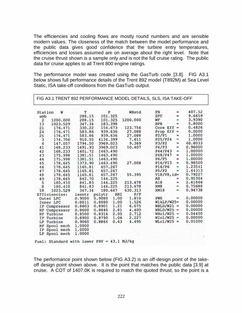
222
The efficiencies and cooling flows are mostly round numbers and are sensible modern values. The closeness of the match between the model performance and the public data gives good confidence that the turbine entry temperatures, efficiencies and losses assumed are on average about the right level. Note that the cruise thrust shown is a sample only and is not the full cruise rating. The public data for cruise applies to all Trent 800 engine ratings. The performance model was created using the GasTurb code [3.8]. FIG A3.1 below shows full performance details of the Trent 892 model (T892M) at Sea Level Static, ISA take-off conditions from the GasTurb output.
The performance point shown below (FIG A3.2) is an off-design point of the take-off design point shown above. It is the point that matches the public data [3.9] at cruise. A COT of 1407.0K is required to match the quoted thrust, so the point is a
FIG A3.1 TRENT 892 PERFORMANCE MODEL DETAILS, SLS, ISA TAKE-OFF

223
much lower non-dimensional operating point than take-off. As well as matching the quoted cruise thrust, the point matches the quoted SFC very closely.
It is also of interest to calculate the combustor outlet temperature (COT) at the cruise flight condition used herein, namely 0.83Mach, 10670m, ISA (where the inlet total temperature is 249.8K) that has the same non-dimensional value as the take-off COT, normalised by inlet total temperature. COT take-off / 288.15 = COT cruise / 248.9 Inserting COT take-off = 1794.5 K gives COT cruise = 1550.3 K (The engine model performance at 1550K COT, 0.83 Mach, 10670m, ISA is shown in APPENDIX 5; it is the basis of the bypass ratio study reported herein).
FIG A3.2 TRENT 892 OFF-DESIGN PERFORMANCE; 0.83 MACH, 10670m, ISA

224
APPENDIX 4 VARIATION OF OPTIMUM FAN PR WITH FORWARD SPEED
FIXED TET AND INLET TEMPERATURE DESIGN POINTS BPR 6
Walsh and Fletcher
For p0 > 22.633 alt = 44330.48 x (1 - ((p0/101.325)^0.1902632))
For alt <11000m t0 = 288.15 - 0.0065*alt
SLS, ISA Flight 0.2M,234.6m, ISA - 0.762C Flight 0.83M, 3651.3m, ISA -11.16C
Opt FPR 1.712 FPR 1.712 opt FPR 1.7175 FPR 1.712 Opt FPR 1.785
Alt m 0 234.6 234.6 3651.3 3651.3
p0 kPa 101.325 98.54 98.54 64.49 64.49
t0 at ISA K 288.15 286.6 286.6 264.4 264.4
Del t0 C 0 -0.762 -0.762 -11.160 -11.160
t0 actual K 288.15 285.86 285.86 253.26 253.26
M 0 0.2 0.2 0.83 0.83
T/t 0 1.000 1.008 1.008 1.138 1.138
P/p 0 1.000 1.0283 1.0283 1.5711 1.571
T2 K 288.15 288.15 288.15 288.15 288.150
P2 kPa 101.325 101.325 101.325 101.325 101.325
W18 kg/s 600 600 600 600 600
W8 kg/s 102.24 102.24 102.24 102.24 102.24
P18 kPa 170.87 170.87 171.42 170.87 178.15
T18 K 341.37 341.37 341.71 341.37 345.88
P18/p0 1.686 1.734 1.740 2.649 2.762
Iter Cp etc P/p crit 1.893 1.893 1.893 1.894 1.893
Iter Cp etc Mach throat 0.897 0.923 0.926 1.000 1.000
P18/p18 1.686 1.734 1.740 1.894 1.893
p18 kPa 101.33 98.54 98.54 90.24 94.10
Iter Cp etc T18/t18 1.1612 1.1705 1.1716 1.2004 1.2003
t18 K 294.0 291.6 291.7 284.4 288.2
t18/1000 0.2940 0.2916 0.2917 0.2844 0.2882
far 0 0 0 0 0
Cp18 kJ/kg.K 1.004 1.003 1.003 1.003 1.003
γ18 1.401 1.401 1.401 1.401 1.401
(γ-1)/2 0.2003 0.2003 0.2003 0.2004 0.2003
γ/(γ-1) 18 3.497 3.496 3.496 3.495 3.496
rho 18 kg/m^3 1.201 1.177 1.177 1.106 1.138
A18 m^2 1.620 1.613 1.608 1.605 1.550
V18 m/s 308.4 315.9 316.9 338.1 340.3
Fg18 kN 185.0 189.5 190.1 244.2 250.1
V18 exp m/s 308.4 315.9 316.9 407.0 416.8
P8 kPa 137.4 137.4 136.1 137.4 121.3
T8 K 866.7 866.7 864.9 866.7 843.5
P8/p0 1.356 1.395 1.381 2.131 1.880
Iter Cp etc P/p crit 8 1.855 1.856 1.856 1.860 1.861
Iter Cp etc Mach throat 8 0.688 0.720 0.709 1.000 1.000
P8/p8 1.356 1.395 1.381 1.860 1.861
p8 kPa 101.33 98.54 98.54 73.90 65.16
Iter Cp etc T8/t8 1.080 1.088 1.085 1.172 1.174
t8 K 802.5 796.7 797.0 739.2 718.8
t8/1000 0.8025 0.7967 0.7970 0.7392 0.719
far 0.0224 0.0224 0.0224 0.0224 0.0224
Cp8 kJ/kg.K 1.136 1.134 1.134 1.119 1.114
γ8 1.338 1.339 1.339 1.345 1.347
(γ-1)/2 8 0.1690 0.1693 0.1693 0.1724 0.1736
γ/(γ-1) 8 3.958 3.953 3.953 3.900 3.881
Mach throat revised 0.688 0.720 0.709 1.000 1.000
rho 8 kg/m^3 0.4400 0.4309 0.4308 0.3483 0.316
A8 m^2 0.6087 0.5959 0.6050 0.5504 0.6150
V8 m/s 381.76 398.12 392.27 533.28 526.26
Fg8 kN 39.03 40.70 40.10 59.70 54.21
V8 exp m/s 381.76 398.12 392.27 583.90 530.29
V18/V8 0.8078 0.7934 0.8078 0.6970 0.7859
V16 / V8 Gasturb 0.8074 0.7930 0.8074 0.6974 0.7872
C0 m/s 340.263 338.910 338.910 318.996 318.996
VTAS m/s 0 67.78 67.78 264.77 264.77
Fgross kN 224.056 230.232 230.237 303.886 304.273
Fdrag kN 0 47.45 47.45 185.34 185.34
Fn kN 224.056 182.784 182.789 118.549 118.937
eta fan x eta LPT isen 0.7926 0.7926 0.7927 0.7926 0.794
1318
2
8

225
APPENDIX 5
TRENT 892 MODEL DATUM PERFORMANCE POINT AT CRUISE FOR STUDIES
Estimated operating performance details of the RR Trent 892 engine are shown on FIG A5.1, below, at cruise. The flight condition is 0.83 Mach, 10670m, ISA, which is the condition at which all the cruise studies herein are done. This is the basic starting point of the T892M.
This point was converted to a design point and then used for as the basis for the studies on varying turbofan bypass ratio – performance, noise, fuel burn and DOC - described in Chapter 3. The core also forms the basis of the open rotor studies of Section 3.6.
FIG A5.1 TRENT 892 ENGINE ESTIMATED PERFORMANCE; 1550K COT, 0.83 MACH, 10670m, ISA OUTPUT FROM GASTURB CODE [3.8]
226
APPENDIX 6 AIR AND POWER OFFTAKES A6.1 PREAMBLE The installed performance quoted in Chapter 3 includes extraction of air and power from the engines for aircraft services. The amounts of these off-takes are listed below. Also shown is the rationale for how the amounts of the off-takes are chosen. The off-takes are discussed in Section 3.1.12.10. The off-takes apply to both the installed cruise design study (Section 3.1) and to the off-design performance used for noise assessment (Section 3.2). A6.2 RATIONALE The off-takes for the datum T892M engine, of cruise bypass ratio 5.98, are calculated based on the aircraft needs, as described below. These off-takes are deemed to apply to the T892M engine with the datum cruise design fan pressure ratio of 1.795. As the cruise design fan pressure ratio is varied at constant bypass ratio, the off-takes are kept constant although the cruise design net thrust varies. At other bypass ratios the off-takes are scaled relative to the datum bypass ratio 5.98 values according to the cruise design thrust of the engine with the optimum fan pressure ratio at that bypass ratio. Again the off-takes are kept constant at each bypass ratio. The aircraft is assumed to be the B777 with maximum seating of 550 and a crew of 10. It has a maximum all-up weight of 660,000lb (299,270 kg) and 2 engines. A6.3 AIR OFFTAKE A value for air off-take commonly used is 1 lb/min per person. For the aircraft assumptions above, this amounts to 2.117 kg/s per engine. This has been rounded to 2.15 kg/s and used for the datum bypass ratio of 5.98. It has been scaled for each bypass ratio, proportional to the cruise net thrust of the optimum engine at each bypass ratio (see TABLE A6.1 below). A6.4 POWER OFFTAKE The value used as datum is a maximum capability of 0.001 kW per kg of all-up aircraft weight [3.16], [3.17]. For the aircraft assumed this gives 299 kW total requirement. Normal use is about 70% giving about 105 kW per engine. This has been rounded to 110 kW for the datum bypass ratio of 5.98 and then scaled in the same way as the air off-take. Please see TABLE A6.1 below.

227
A6.5 RESULTS
TABLE A6.1 AIR AND POWER OFFTAKES
BYPASS RATIO
5.98 10 15 20 25 30
CRUISE THRUST
kN 75.98 81.12 83.86 84.88 85.10 84.86
AIR OFFTAKE
kg/s 2.15 2.3 2.37 2.4 2.41 2.4
POWER OFFTAKE
kW 110 117 121 123 123 123
End of Appendix 6

228
APPENDIX 7
INSTALLATION DESIGN AND PERFORMANCE AT CRUISE
TEXT REFERENCE 3.1.12.11
This Appendix gives full details of the calculations of installation losses at cruise for long and short cowls and for open rotors.
The columns filled in yellow are those having the optimum fan pressure ratio for that bypass ratio, with no installation losses.
The columns filled in pink are those having closely the optimum fan pressure ratio for that bypass ratio, with full installation losses.
The methods used in the calculations are described in the main text in Section 3.1.12.
SHEETS 1 TO 4 LONG AND SHORT COWL BYPASS RATIOS 5.98, 10, 15
Pages 229 to 232
SHEETS 5 TO 8 LONG AND SHORT COWL BYPASS RATIOS 20, 25, 30
Pages 233 to 236
SHEET 9 OPEN ROTORS BYPASS RATIOS 30, 50, 80
Page 237
The methods used to obtain installed performance at take-off are basically the
same and so details are not included in this document.

APPENDIX 7 SHEETS 1 TO 4 PAGES 229 to 232 INSTALLATION DESIGN AND CRUISE LOSSES BPR 5.98, 10, 15
FPR b = Optimum fan outer pressure ratio, bare engine
FPR i = Optimum fan outer pressure ratio, intalled
ASSUMPTIONS Fan inlet hub/tip 0.3 Afterbody boat-tail angle 14deg Strut behind LPT adds 0.25 m length
Duct axial velocity 140 m/s for BPR 6 and graded larger at higher BPR to keep fan outlet hub/tip reasonable Cowl boat-tail angle 11deg Graded allowance made for fan root PR being less than tip
BPD Loss proportional to wetted area x density/bypass flow Nose cone angle 27.5 deg Fan entry Mach number constant with BPR
Datum loss at BPR = 6 is 1.508%DP/P (1.5% at T/O) Angle of duct to core entry 10 deg Fan tip speed same for all fans
Area of duct does not change significantly with length Intake L/D =0.5 LPT stage loading constant - adds or reduces stage numbers
Static pressure behind fan from bypass parameters Cowl ends at LPT exit plane
BPR 5.98 5.98 5.98 5.98 5.98 5.98 10 10 10 10 10 10 15 15 15 15 15FOPR 1.795 1.4 1.6 1.7 1.74 1.9 1.3 1.4 1.45 1.5 1.57 1.6 1.2 1.25 1.3 1.33 1.35
BYPASS DUCT LOSS TRENT 892 FPR i FPR i FPR b FPR i FPR bAltitude km 10.67 10.67 10.67 10.67 10.67 10.67 10.67 10.67 10.67 10.67 10.67 10.67 10.67 10.67 10.67 10.67 10.67
Mach 0.83 0.83 0.83 0.83 0.83 0.83 0.83 0.83 0.83 0.83 0.83 0.83 0.83 0.83 0.83 0.83 0.83
P0 kPa 37.45 37.45 37.45 37.45 37.45 37.45 37.45 37.45 37.45 37.45 37.45 37.45 37.45 37.45 37.45 37.45 37.45
T0 K 248.9 248.9 248.9 248.9 248.9 248.9 248.9 248.9 248.9 248.9 248.9 248.9 248.9 248.9 248.9 248.9 248.9
P2/P0 1 1 1 1 1 1 1 1 1 1 1 1 1 1 1 1 1
P2 kPa 37.45 37.45 37.45 37.45 37.45 37.45 37.45 37.45 37.45 37.45 37.45 37.45 37.45 37.45 37.45 37.45 37.45
Mach station 2 0.655 0.655 0.655 0.655 0.655 0.655 0.655 0.655 0.655 0.655 0.655 0.655 0.655 0.655 0.655 0.655 0.655
T2/t2 1.086 1.086 1.086 1.086 1.086 1.086 1.086 1.086 1.086 1.086 1.086 1.086 1.086 1.086 1.086 1.086 1.086
t2 K 229.3 229.3 229.3 229.3 229.3 229.3 229.3 229.3 229.3 229.3 229.3 229.3 229.3 229.3 229.3 229.3 229.3
P2/p2 1.334 1.334 1.334 1.334 1.334 1.334 1.334 1.334 1.334 1.334 1.334 1.334 1.334 1.334 1.334 1.334 1.334
p2 kPa 28.08 28.08 28.08 28.08 28.08 28.08 28.08 28.08 28.08 28.08 28.08 28.08 28.08 28.08 28.08 28.08 28.08
rho 2 (density) kg/m^3 0.427 0.427 0.427 0.427 0.427 0.427 0.427 0.427 0.427 0.427 0.427 0.427 0.427 0.427 0.427 0.427 0.427
c2 (speed of sound) m/s 303.52 303.52 303.52 303.52 303.52 303.52 303.52 303.52 303.52 303.52 303.52 303.52 303.52 303.52 303.52 303.52 303.52
V2 (velocity at fan face) m/s 198.75 198.75 198.75 198.75 198.75 198.75 198.75 198.75 198.75 198.75 198.75 198.75 198.75 198.75 198.75 198.75 198.75
W2 kg/s 473.15 473.15 473.15 473.15 473.15 473.15 744.62 744.62 744.62 744.62 744.62 744.62 1084.54 1084.54 1084.54 1084.54 1084.54
A2 in m^2 5.579 5.579 5.579 5.579 5.579 5.579 8.780 8.780 8.780 8.780 8.780 8.780 12.789 12.789 12.789 12.789 12.789
h/t 2 0.3 0.3 0.3 0.3 0.3 0.3 0.3 0.3 0.3 0.3 0.3 0.3 0.3 0.3 0.3 0.3 0.3
Atip in 6.131 6.131 6.131 6.131 6.131 6.131 9.649 9.649 9.649 9.649 9.649 9.649 14.054 14.054 14.054 14.054 14.054
Dtip in m 2.794 2.794 2.794 2.794 2.794 2.794 3.505 3.505 3.505 3.505 3.505 3.505 4.230 4.230 4.230 4.230 4.230
Dtip in ins 110.000 110.0 110.0 110.0 110.0 110.0 138.0 138.0 138.0 138.0 138.0 138.0 166.5 166.5 166.5 166.5 166.5
Dtip out/ Dtip in 0.95 1.0000 0.9780 0.9657 0.9588 0.9337 1.0000 0.9940 0.9889 0.9818 0.9708 0.9665 1.0000 1.0000 1.0000 0.9978 0.9954
Dtip out 2.654 2.794 2.733 2.698 2.679 2.609 3.505 3.484 3.466 3.441 3.403 3.388 4.230 4.230 4.230 4.221 4.211
Atip out 5.533 6.131 5.864 5.718 5.636 5.345 9.649 9.533 9.436 9.301 9.094 9.013 14.054 14.054 14.054 13.992 13.925
T13 K 298.99 276.61 288.42 293.94 296.09 304.35 270.26 276.61 279.66 282.65 286.71 288.42 263.57 266.96 270.25 272.2 273.48
V13 to set fan root exit dia m/s 140 150.4 142.4 140.0 140.0 140 163.0 155.0 152.5 151 149.8 149.20 174.1 167.1 160.8 158.4 157.3
t13 K 289.19 265.3 278.3 284.1 286.3 294.6 257.0 264.6 268.0 271.2 275.5 277.3 248.4 253.0 257.3 259.7 261.1
T13/t13 1.034 1.043 1.036 1.034 1.034 1.033 1.052 1.045 1.043 1.042 1.041 1.040 1.061 1.055 1.050 1.048 1.047
Mach 13 0.412 0.462 0.427 0.415 0.414 0.408 0.508 0.476 0.466 0.458 0.451 0.448 0.552 0.525 0.501 0.492 0.487
P13/p13 1.124 1.157 1.133 1.126 1.125 1.121 1.193 1.168 1.160 1.155 1.150 1.148 1.230 1.207 1.187 1.180 1.176
P13 kPa 67.217 52.426 59.915 63.660 65.158 71.149 48.681 52.426 54.298 56.170 58.792 59.915 44.936 46.809 48.681 49.804 50.553
p13 kPa 59.817 45.303 52.862 56.536 57.917 63.448 40.808 44.880 46.798 48.632 51.125 52.205 36.524 38.786 41.006 42.222 42.992
rho 13 kg/m^3 0.721 0.595 0.662 0.693 0.705 0.751 0.553 0.591 0.608 0.625 0.647 0.656 0.512 0.534 0.555 0.567 0.574
A fan exit m^2 4.689 5.289 5.020 4.875 4.795 4.503 8.256 8.129 8.026 7.894 7.687 7.608 12.160 12.150 12.147 12.084 12.018
A fan root out m^2 0.844 0.842 0.844 0.843 0.842 0.842 1.393 1.405 1.410 1.407 1.406 1.405 1.894 1.903 1.907 1.907 1.906
Droot fan exit m 1.037 1.035 1.037 1.036 1.035 1.036 1.332 1.337 1.340 1.338 1.338 1.338 1.553 1.557 1.558 1.558 1.558
h/t fan out 0.391 0.371 0.379 0.384 0.386 0.397 0.380 0.384 0.387 0.389 0.393 0.395 0.367 0.368 0.368 0.369 0.370
rho Ratio for Pinner<Pouter goal Dsplit 0.700 0.781 0.750 0.720 0.710 0.665 0.789 0.785 0.780 0.770 0.736 0.726 0.820 0.815 0.812 0.807 0.800
Acore m^2 0.960 0.971 0.959 0.969 0.967 0.970 0.952 0.941 0.935 0.932 0.950 0.952 0.927 0.932 0.935 0.936 0.939
Asplitter m^2 1.80 1.81 1.80 1.81 1.81 1.81 2.34 2.35 2.35 2.34 2.36 2.36 2.82 2.83 2.84 2.84 2.85
Dsplitter m 1.52 1.52 1.52 1.52 1.52 1.52 1.73 1.73 1.73 1.73 1.73 1.73 1.90 1.90 1.90 1.90 1.90
LENGTH OF BPD, L m 3.10 2.97 3.00 3.05 3.07 3.15 3.65 3.79 3.85 3.90 3.97 4.00 4.46 4.56 4.69 4.75 4.79
Awet inner m^2 14.76 14.17 14.28 14.56 14.64 15.03 19.81 20.58 20.90 21.14 21.60 21.77 26.55 27.22 28.03 28.39 28.64
Awet outer m^2 25.85 26.07 25.75 25.85 25.84 25.82 40.19 41.48 41.92 42.16 42.44 42.57 59.27 60.60 62.33 62.98 63.36
Awet total 40.61 40.24 40.03 40.41 40.48 40.85 60.00 62.06 62.82 63.31 64.04 64.34 85.82 87.82 90.35 91.38 92.01
Dyn Hd = 0.5xrhoxV^2 Pa 7062.9 6725.3 6710.7 6794.2 6907.9 7355.4 7350.5 7099.4 7074.1 7121.9 7255.1 7301.4 7764.1 7457.7 7178.4 7108.0 7097.6
Dyn Hd x A wet/1000 286.82 270.65 268.65 274.55 279.60 300.46 441.05 440.61 444.42 450.87 464.63 469.78 666.34 654.90 648.59 649.51 653.01
Divide by Wbypass 0.708 0.668 0.663 0.677 0.690 0.741 0.652 0.651 0.657 0.666 0.686 0.694 0.655 0.644 0.638 0.639 0.642
k (x1000 in effect) 2.1313 2.1313 2.1313 2.1313 2.1313 2.1313 2.1313 2.1313 2.1313 2.1313 2.1313 2.1313 2.1313 2.1313 2.1313 2.1313 2.1313
L
13 182

BP DUCT LOSS %DP/P 1.508 1.423 1.413 1.444 1.470 1.580 1.389 1.387 1.399 1.420 1.463 1.479 1.397 1.373 1.360 1.361 1.369
Droot in fan entry m 0.838 0.838 0.838 0.838 0.838 0.838 1.052 1.052 1.052 1.052 1.052 1.052 1.269 1.269 1.269 1.269 1.269
FAN COWL THICKNESS m 0.250 0.250 0.250 0.250 0.250 0.250 0.250 0.250 0.250 0.250 0.250 0.250 0.250 0.250 0.250 0.250 0.250
FAN COWL MAX RAD m 1.647 1.647 1.647 1.647 1.647 1.647 2.003 2.003 2.003 2.003 2.003 2.003 2.365 2.365 2.365 2.365 2.365
POD DRAG CALCS BASED ON WALSH AND FLETCHER P251 F5.5.1 AND F5.5.2
FAN COWLFlight Mach 0.830 0.830 0.830 0.830 0.830 0.830 0.830 0.830 0.830 0.830 0.830 0.830 0.830 0.830 0.830 0.830 0.830
Altitude km 10.670 10.670 10.670 10.670 10.670 10.670 10.670 10.670 10.670 10.670 10.670 10.670 10.670 10.670 10.670 10.670 10.670
p0 kPa 23.835 23.835 23.835 23.835 23.835 23.835 23.835 23.835 23.835 23.835 23.835 23.835 23.835 23.835 23.835 23.835 23.835
t0 K 218.8 218.8 218.8 218.8 218.8 218.8 218.8 218.8 218.8 218.8 218.8 218.8 218.8 218.8 218.8 218.8 218.8
rho0 kg/m^3 0.380 0.380 0.380 0.380 0.380 0.380 0.380 0.380 0.380 0.380 0.380 0.380 0.380 0.380 0.380 0.380 0.380
c0 m/s 296.50 296.50 296.50 296.50 296.50 296.50 296.50 296.50 296.50 296.50 296.50 296.50 296.50 296.50 296.50 296.50 296.50
VTAS m/s 246.09 246.09 246.09 246.09 246.09 246.09 246.09 246.09 246.09 246.09 246.09 246.09 246.09 246.09 246.09 246.09 246.09
FAN COWL MAX RAD m 1.647 1.647 1.647 1.647 1.647 1.647 2.003 2.003 2.003 2.003 2.003 2.003 2.365 2.365 2.365 2.365 2.365
FAN COWL LENGTH (drawing) m 5.40 5.17 5.30 5.35 5.37 5.44 6.66 6.79 6.85 6.90 6.97 7.00 7.91 8.04 8.15 8.21 8.25
Cowl area m^2 55.84 53.55 54.82 55.37 55.57 56.33 83.82 85.46 86.19 86.87 87.75 88.11 117.59 119.44 121.11 122.01 122.59
Factor C (Walsh and Fletcher) 0.003 0.003 0.003 0.003 0.003 0.003 0.003 0.003 0.003 0.003 0.003 0.003 0.003 0.003 0.003 0.003 0.003
Interference factor 1.200 1.200 1.200 1.200 1.200 1.200 1.200 1.200 1.200 1.200 1.200 1.200 1.200 1.200 1.200 1.200 1.200
COWL DRAG kN 2.311 2.216 2.268 2.291 2.299 2.331 3.468 3.536 3.566 3.594 3.631 3.646 4.866 4.942 5.011 5.049 5.073Fn bare kN 75.98 68.25 73.95 75.42 75.76 75.63 74.60 79.49 80.76 81.12 79.39 77.04 75.76 80.54 83.35 83.86 83.45
DRAG/Fn % 3.041 3.247 3.068 3.038 3.035 3.082 4.649 4.448 4.416 4.431 4.574 4.732 6.422 6.137 6.012 6.020 6.079Fn/W2 160.6 144.2 156.3 159.4 160.1 159.8 100.2 106.8 108.5 108.9 106.6 103.5 69.9 74.3 76.9 77.3 76.9
INTAKE HIGHLIGHT
Mass flow increase at climb Factor 1.060 1.060 1.060 1.060 1.060 1.060 1.060 1.060 1.060 1.060 1.060 1.060 1.060 1.060 1.060 1.060 1.060
W2 climb kg/s 501.54 501.54 501.54 501.54 501.54 501.54 789.30 789.30 789.30 789.30 789.30 789.30 1149.62 1149.62 1149.62 1149.62 1149.62
A highlight m^2 5.37 5.37 5.37 5.37 5.37 5.37 8.45 8.45 8.45 8.45 8.45 8.45 12.31 12.31 12.31 12.31 12.31
D highlight m 2.61 2.61 2.61 2.61 2.61 2.61 3.28 3.28 3.28 3.28 3.28 3.28 3.96 3.96 3.96 3.96 3.96
LP TURBINE AND AFTERBODYD LPT TIP out goal length/stage m 1.845 1.636 1.752 1.802 1.821 1.890 1.922 2.045 2.100 2.151 2.217 2.244 2.149 2.267 2.372 2.430 2.467
LPT EXIT AREA to Centre m^2 2.674 2.103 2.411 2.550 2.603 2.804 2.901 3.285 3.464 3.634 3.861 3.955 3.627 4.036 4.421 4.638 4.781
Radius LPT TIP out m 0.923 0.818 0.876 0.901 0.910 0.945 0.961 1.023 1.050 1.076 1.109 1.122 1.075 1.134 1.186 1.215 1.234
ADD TO RADIUS TO CLEAR LPT m 0.100 0.100 0.100 0.100 0.100 0.100 0.110 0.110 0.110 0.110 0.110 0.110 0.120 0.120 0.120 0.120 0.120
RADIUS BP NOZ INNER m 1.023 0.918 0.976 1.001 1.010 1.045 1.071 1.133 1.160 1.186 1.219 1.232 1.195 1.254 1.306 1.335 1.354
A BYPASS NOZZLE INNER m^2 3.286 2.648 2.993 3.148 3.207 3.429 3.604 4.029 4.227 4.415 4.665 4.768 4.483 4.936 5.360 5.599 5.756
A18 m^2 2.619 3.229 2.885 2.742 2.688 2.496 5.748 5.400 5.242 5.095 4.902 4.825 9.227 8.912 8.622 8.458 8.352
A BYPASS NOZZLE OUTER m^2 5.904 5.878 5.879 5.889 5.895 5.925 9.352 9.429 9.470 9.510 9.568 9.593 13.709 13.849 13.983 14.057 14.109
D BYPASS NOZZLE OUTER m 2.742 2.736 2.736 2.738 2.740 2.747 3.451 3.465 3.472 3.480 3.490 3.495 4.178 4.199 4.219 4.231 4.238
Distance core LE to BP nozzle m 3.505 3.284 3.407 3.459 3.479 3.552 3.587 3.717 3.775 3.829 3.899 3.928 3.827 3.952 4.064 4.125 4.164
A8 m^2 0.953 0.514 0.704 0.823 0.875 1.131 0.634 0.853 0.991 1.172 1.707 2.324 0.653 0.827 1.058 1.275 1.517
LPT exit h/t 0.500 0.500 0.500 0.500 0.500 0.500 0.500 0.500 0.500 0.500 0.500 0.500 0.500 0.500 0.500 0.500 0.500
A LPT OUT m^2 2.006 1.577 1.808 1.913 1.952 2.103 2.176 2.463 2.598 2.725 2.896 2.966 2.720 3.027 3.316 3.478 3.586
A8/(A LPT out) 0.475 0.326 0.389 0.430 0.448 0.538 0.292 0.346 0.382 0.430 0.589 0.784 0.240 0.273 0.319 0.367 0.423
D8 m 1.102 0.809 0.947 1.023 1.056 1.200 0.899 1.042 1.124 1.222 1.474 1.720 0.912 1.026 1.160 1.274 1.390
LPT Tin 46 K 998.67 998.67 998.67 998.67 998.67 998.67 998.67 998.67 998.67 998.67 998.67 998.67 998.67 998.67 998.67 998.67 998.67
LPT Tout 49 K 707.17 825.93 763.68 734.23 722.74 678.19 783.95 727.53 700.08 673.11 636.08 620.46 778.44 733.21 688.75 662.41 644.99
LPT TEMPERATURE DROP C 291.50 172.74 234.99 264.44 275.93 320.48 214.72 271.14 298.59 325.56 362.59 378.21 220.23 265.46 309.92 336.26 353.68
LPT MEAN T K 852.92 912.30 881.18 866.45 860.71 838.43 891.31 863.10 849.38 835.89 817.38 809.57 888.56 865.94 843.71 830.54 821.83
LPT MEAN T / 1000 0.853 0.912 0.881 0.866 0.861 0.838 0.891 0.863 0.849 0.836 0.817 0.810 0.889 0.866 0.844 0.831 0.822
far LPT Mean 0.01816 0.01816 0.01816 0.01816 0.01816 0.01816 0.01816 0.01816 0.01816 0.01816 0.01816 0.01816 0.01816 0.01816 0.01816 0.01816 0.01816
Cp mean J/kg.K 1141.6 1155.8 1148.5 1144.9 1143.5 1138.1 1150.9 1144.1 1140.8 1137.5 1132.8 1130.9 1150.2 1144.8 1139.4 1136.1 1133.9
T 5 K 707.1 824.2 762.6 733.4 722.0 677.9 782.6 726.8 699.6 672.8 636.2 620.7 777.2 732.4 688.3 662.2 645.0
T / 1000 0.7071 0.8242 0.7626 0.7334 0.7220 0.6779 0.7826 0.7268 0.6996 0.6728 0.6362 0.6207 0.7772 0.7324 0.6883 0.6622 0.6450
far 5 0.01798 0.01798 0.01798 0.01798 0.01798 0.01798 0.01798 0.01798 0.01798 0.01798 0.01798 0.01798 0.01798 0.01798 0.01798 0.01798 0.01798
Cp 5 J/kg.K 1104.1 1134.3 1118.5 1110.9 1108.0 1096.4 1123.7 1109.2 1102.1 1095.0 1085.4 1081.4 1122.3 1110.7 1099.1 1092.3 1087.7
γ/(γ-1) 5 3.847 3.952 3.897 3.871 3.860 3.820 3.915 3.865 3.840 3.815 3.782 3.768 3.911 3.870 3.830 3.806 3.790
γ 5 1.351 1.339 1.345 1.348 1.350 1.355 1.343 1.349 1.352 1.355 1.359 1.361 1.344 1.348 1.353 1.356 1.358
Mach LPT out 5 GOAL SEEK 0.2911 0.1947 0.2346 0.2609 0.2731 0.3313 0.1731 0.2070 0.2293 0.2565 0.3047 0.3302 0.1416 0.1618 0.1896 0.2109 0.2275
T/t 5 1.015 1.006 1.009 1.012 1.013 1.019 1.005 1.007 1.009 1.012 1.017 1.020 1.003 1.005 1.006 1.008 1.009
t 5 K 696.75 818.97 755.39 724.80 712.71 664.93 778.64 721.36 693.14 665.07 625.73 608.71 774.51 729.05 683.99 657.03 639.06
P 5 kPa 48.13 96.62 67.78 56.86 53.01 40.03 76.27 54.59 46.04 38.73 30.27 27.18 73.88 56.51 42.84 36.16 32.19
P/p 5 1.058 1.026 1.038 1.047 1.051 1.076 1.020 1.029 1.036 1.045 1.065 1.076 1.014 1.018 1.025 1.031 1.036
p 5 kPa 45.473 94.202 65.332 54.324 50.421 37.189 74.750 53.037 44.437 37.053 28.430 25.252 72.892 55.523 41.816 35.085 31.086
rho 5 kg/m^3 0.2274 0.4008 0.3014 0.2612 0.2465 0.1949 0.3345 0.2562 0.2234 0.1941 0.1583 0.1445 0.3279 0.2654 0.2130 0.1861 0.1695
W 5 kg/s 69.03 69.03 69.03 69.03 69.03 69.03 69.03 69.03 69.03 69.03 69.03 69.03 69.03 69.03 69.03 69.03 69.03
c 5 m/s 519.82 560.95 540.02 529.60 525.41 508.43 547.83 528.48 518.63 508.60 494.10 487.66 546.50 531.17 515.44 505.74 499.15

Rad LPT exit root m 0.461 0.409 0.438 0.451 0.455 0.472 0.481 0.511 0.525 0.538 0.554 0.561 0.537 0.567 0.593 0.608 0.617
LPT exit AREA A5 m^2 2.006 1.577 1.808 1.913 1.952 2.103 2.176 2.463 2.598 2.725 2.896 2.966 2.720 3.027 3.316 3.478 3.586
Va 5 from guessed M 5 m/s 151.32 109.21 126.69 138.17 143.49 168.44 94.83 109.40 118.92 130.47 150.55 161.03 77.38 85.94 97.73 106.66 113.56
A 5 check m^2 2.006 1.577 1.808 1.913 1.952 2.103 2.176 2.463 2.598 2.725 2.896 2.966 2.720 3.027 3.316 3.478 3.586
Fan tip speed m/s 400.0 400.0 400.0 400.0 400.0 400.0 400.0 400.0 400.0 400.0 400.0 400.0 400.0 400.0 400.0 400.0 400.0
LPT mean dia m 1.183 1.105 1.148 1.167 1.174 1.200 1.212 1.258 1.279 1.298 1.323 1.333 1.297 1.341 1.381 1.403 1.416
LPT mean blade speed m/s 169.40 158.18 164.40 167.07 168.07 171.77 138.31 143.58 145.93 148.12 150.95 152.10 122.66 126.84 130.58 132.62 133.94
LPT exit mean blade speed m/s 198.14 175.69 188.14 193.49 195.48 202.89 164.51 175.03 179.74 184.11 189.77 192.07 152.41 160.78 168.26 172.34 174.98
Va/U LPT Mean 0.893 0.690 0.771 0.827 0.854 0.981 0.686 0.762 0.815 0.881 0.997 1.059 0.631 0.678 0.748 0.804 0.848
Loading ΔH/U^2 11.597 7.980 9.985 10.847 11.170 12.361 12.917 15.048 15.995 16.880 18.027 18.489 16.837 18.889 20.709 21.721 22.355
Loading last stage 1.600 1.600 1.600 1.600 1.600 1.600 1.600 1.600 1.600 1.600 1.600 1.600 1.600 1.600 1.600 1.600 1.600
Loading all except last st 9.997 6.380 8.385 9.247 9.570 10.761 11.317 13.448 14.395 15.280 16.427 16.889 15.237 17.289 19.109 20.121 20.755
Loading /stage except last 2.498 2.498 2.498 2.498 2.498 2.498 2.498 2.498 2.498 2.498 2.498 2.498 2.498 2.498 2.498 2.498 2.498
Stages 5.00 3.6 4.4 4.7 4.8 5.3 5.5 6.4 6.8 7.1 7.6 7.8 7.1 7.9 8.6 9.1 9.3
LPT LENGTH m 0.765 0.544 0.667 0.719 0.739 0.812 0.847 0.977 1.035 1.089 1.159 1.188 1.087 1.212 1.324 1.385 1.424
Length/stage m 0.153 0.153 0.153 0.153 0.153 0.153 0.153 0.153 0.153 0.153 0.153 0.153 0.153 0.153 0.153 0.153 0.153
AFTERBODY LENGTH m 2.25 2.9 2.55 2.4 2.35 2.1 3.15 2.9 2.79 2.65 2.36 2.07 3.62 3.5 3.38 3.32 3.28
Distance of core nozzle from core inlet m 5.755 6.184 5.957 5.859 5.829 5.652 6.737 6.617 6.565 6.479 6.259 5.998 7.447 7.452 7.444 7.445 7.444
D8 repeat m 1.102 0.809 0.947 1.023 1.056 1.200 0.899 1.042 1.124 1.222 1.474 1.720 0.912 1.026 1.160 1.274 1.390
MEAN AFTERBODY DIA (DWG) m 1.7 1.48 1.57 1.63 1.65 1.73 1.7 1.85 1.95 2.0 2.08 2.12 1.78 1.9 2.05 2.1 2.16
Afterbody area m^2 12.017 13.484 12.577 12.290 12.182 11.413 16.823 16.855 17.092 16.650 15.421 13.787 20.243 20.892 21.768 21.903 22.258
W18 kg/s 405.37 405.37 405.37 405.37 405.37 405.37 677.84 677.84 677.84 677.84 677.84 677.84 1016.76 1016.76 1016.76 1016.76 1016.76
T18 K 298.99 276.61 288.42 293.94 296.09 304.35 270.26 276.61 279.66 282.65 286.71 288.42 263.57 266.96 270.25 272.20 273.48
P18 kPa 66.20 51.63 59.01 62.70 64.18 70.08 47.95 51.64 53.48 55.32 57.91 59.01 44.26 46.10 47.95 49.05 49.79
P18/p0 2.778 2.166 2.476 2.631 2.692 2.940 2.012 2.166 2.244 2.321 2.429 2.476 1.857 1.934 2.012 2.058 2.089
PR crit 1.893 1.893 1.893 1.893 1.893 1.893 1.893 1.893 1.893 1.893 1.893 1.893 1.893 1.893 1.893 1.893 1.893
CHOKED? Y Y Y Y Y Y Y Y Y Y Y Y N Y Y Y Y
Mthroat 18 1 1 1 1 1 1 1 1 1 1 1 1 0.9840 1 1 1 1
P18/p18 1.893 1.893 1.893 1.893 1.893 1.893 1.893 1.893 1.893 1.893 1.893 1.893 1.857 1.893 1.893 1.893 1.893
p18 kPa 34.97 27.28 31.17 33.12 33.90 37.02 25.33 27.28 28.25 29.23 30.59 31.17 23.84 24.36 25.33 25.91 26.30
A18 m^2 2.62 3.23 2.89 2.74 2.69 2.50 5.75 5.40 5.24 5.09 4.90 4.82 9.23 8.91 8.62 8.46 8.35
T18/t18 1.20 1.20 1.20 1.20 1.20 1.20 1.20 1.20 1.20 1.20 1.20 1.20 1.19 1.20 1.20 1.20 1.20
t18 K 249.2 230.5 240.4 245.0 246.7 253.6 225.2 230.5 233.1 235.5 238.9 240.4 220.9 222.5 225.2 226.8 227.9
c18 m/s 316.4 304.3 310.8 313.7 314.9 319.2 300.8 304.3 306.0 307.6 309.8 310.8 297.9 299.0 300.8 301.9 302.6
V18 m/s 316.4 304.3 310.8 313.7 314.9 319.2 300.8 304.3 306.0 307.6 309.8 310.8 293.1 299.0 300.8 301.9 302.6
Fg 18 kN 157.43 134.48 147.15 152.64 154.70 162.32 212.50 224.88 230.58 235.99 243.14 246.06 298.03 308.63 318.74 324.54 328.30
V18 exp m/s 388.4 331.8 363.0 376.5 381.6 400.4 313.5 331.8 340.2 348.2 358.7 363.0 293.1 303.5 313.5 319.2 322.9
rho 18 kg/m^3 0.4891 0.4123 0.4519 0.4712 0.4787 0.5086 0.3919 0.4123 0.4224 0.4323 0.4461 0.4519 0.3760 0.3815 0.3919 0.3981 0.4022
Factor C (Walsh and Fletcher) 0.003 0.003 0.003 0.003 0.003 0.003 0.003 0.003 0.003 0.003 0.003 0.003 0.003 0.003 0.003 0.003 0.003
Interference factor 1.200 1.200 1.200 1.200 1.200 1.200 1.200 1.200 1.200 1.200 1.200 1.200 1.200 1.200 1.200 1.200 1.200
AFTERBODY DRAG kN 1.596 1.101 1.348 1.478 1.529 1.675 1.166 1.377 1.504 1.571 1.593 1.478 1.177 1.322 1.509 1.599 1.680
AFTERBODY DRAG % Fn % Fn 2.100 1.614 1.823 1.959 2.018 2.215 1.563 1.732 1.862 1.936 2.007 1.918 1.554 1.641 1.810 1.907 2.013
COWL DRAG kN 2.311 2.216 2.268 2.291 2.299 2.331 3.468 3.536 3.566 3.594 3.631 3.646 4.866 4.942 5.011 5.049 5.073
COWL DRAG % NET THRUST % Fn 3.04 3.25 3.07 3.04 3.04 3.08 4.65 4.45 4.42 4.43 4.57 4.73 6.42 6.14 6.01 6.02 6.08
TOTAL DRAG kN 3.91 3.32 3.62 3.77 3.83 4.01 4.63 4.91 5.07 5.17 5.22 5.12 6.04 6.26 6.52 6.65 6.75
NET THRUST, Fn, BARE kN 75.98 68.25 73.95 75.42 75.76 75.63 74.60 79.49 80.76 81.12 79.39 77.04 75.76 80.54 83.35 83.86 83.45
TOTAL DRAG % NET THRUST % Fn 5.14 4.86 4.89 5.00 5.05 5.30 6.21 6.18 6.28 6.37 6.58 6.65 7.98 7.78 7.82 7.93 8.09
NET THRUST, INSTALLED kN 70.84 63.39 69.06 70.42 70.71 70.33 68.39 73.31 74.48 74.75 72.81 70.39 67.78 72.76 75.53 75.93 75.36
Fn/W2 160.58 144.25 156.29 159.40 160.12 159.84 100.19 106.75 108.46 108.94 106.62 103.46 69.85 74.26 76.85 77.32 76.94
BP DUCT LOSS %DP/P 1.508 1.423 1.413 1.444 1.470 1.580 1.389 1.387 1.399 1.420 1.463 1.479 1.397 1.373 1.360 1.361 1.369
FOPR 1.795 1.4 1.6 1.7 1.74 1.9 1.3 1.4 1.45 1.5 1.57 1.6 1.2 1.25 1.3 1.33 1.35

FOPR 1.795 1.4 1.6 1.7 1.74 1.9 1.3 1.4 1.45 1.5 1.57 1.6 1.2 1.25 1.3 1.33 1.35
BPR 5.98 10 15
Fn bare kN 75.98 68.25 73.95 75.42 75.76 75.63 74.60 79.49 80.76 81.12 79.39 77.04 75.76 80.54 83.35 83.86 83.45
LONG COWLLONG COWL LENGTH m 5.396 5.175 5.298 5.350 5.370 5.443 6.662 6.792 6.850 6.904 6.974 7.003 7.913 8.038 8.150 8.211 8.250
LONG COWL AFTERBODY LENGTH m 2.25 2.9 2.55 2.4 2.35 2.1 3.15 2.9 2.79 2.65 2.36 2.07 3.62 3.5 3.38 3.32 3.28
LONG COWL BYPASS DUCT LENGTH m 3.10 2.97 3.00 3.05 3.07 3.15 3.65 3.79 3.85 3.90 3.97 4.00 4.46 4.56 4.69 4.75 4.79
MAX COWL DIA m 3.2940 3.2940 3.2940 3.2940 3.2940 3.2940 4.0050 4.0050 4.0050 4.0050 4.0050 4.0050 4.7301 4.7301 4.7301 4.7301 4.7301
AFTERBODY MEAN DIA m 1.70 1.48 1.57 1.63 1.65 1.73 1.70 1.85 1.95 2.00 2.08 2.12 1.78 1.90 2.05 2.10 2.16
COWL DRAG kN 2.31 2.22 2.27 2.29 2.30 2.33 3.47 3.54 3.57 3.59 3.63 3.65 4.87 4.94 5.01 5.05 5.07
COWL DRAG % Fn 3.04 3.25 3.07 3.04 3.04 3.08 4.65 4.45 4.42 4.43 4.57 4.73 6.42 6.14 6.01 6.02 6.08
AFTERBODY DRAG kN 1.60 1.10 1.35 1.48 1.53 1.68 1.17 1.38 1.50 1.57 1.59 1.48 1.18 1.32 1.51 1.60 1.68
AFTERBODY DRAG % Fn 2.10 1.61 1.82 1.96 2.02 2.22 1.56 1.73 1.86 1.94 2.01 1.92 1.55 1.64 1.81 1.91 2.01
TOTAL DRAG kN 3.91 3.32 3.62 3.77 3.83 4.01 4.63 4.91 5.07 5.17 5.22 5.12 6.04 6.26 6.52 6.65 6.75
TOTAL DRAG % Fn 5.14 4.86 4.89 5.00 5.05 5.30 6.21 6.18 6.28 6.37 6.58 6.65 7.98 7.78 7.82 7.93 8.09
BYPASS LOSS %DP/P 1.508 1.423 1.413 1.444 1.470 1.580 1.389 1.387 1.399 1.420 1.463 1.479 1.397 1.373 1.360 1.361 1.369
BYPASS PR LONG COWL 0.9849 0.9858 0.9859 0.9856 0.9853 0.9842 0.9861 0.9861 0.9860 0.9858 0.9854 0.9852 0.9860 0.9863 0.9864 0.9864 0.9863
SHORT COWLSHORT COWL LENGTH = max dia 3.294 3.294 3.294 3.294 3.294 3.294 4.005 4.005 4.005 4.005 4.005 4.005 4.730 4.730 4.730 4.730 4.730
COWL LENGTH REDUCTION m 2.102 1.881 2.004 2.056 2.076 2.149 2.657 2.787 2.845 2.899 2.969 2.998 3.183 3.308 3.420 3.480 3.520
BYPASS DUCT LENGTH m 0.998 1.089 0.996 0.994 0.994 1.001 0.993 1.003 1.005 1.001 1.001 1.002 1.277 1.252 1.270 1.270 1.270
AFTERBODY LENGTH m 4.352 4.781 4.554 4.456 4.426 4.249 5.807 5.687 5.635 5.549 5.329 5.068 6.803 6.808 6.800 6.800 6.800
COWL DRAG kN 1.410 1.410 1.410 1.410 1.410 1.410 2.085 2.085 2.085 2.085 2.085 2.085 2.908 2.908 2.908 2.908 2.908
COWL DRAG % Fn 1.856 2.067 1.907 1.870 1.862 1.865 2.795 2.623 2.582 2.570 2.626 2.707 3.839 3.611 3.489 3.468 3.485
BYPASS LOSS % DP/P 0.4853 0.5218 0.4691 0.4702 0.4760 0.5019 0.3780 0.3672 0.3653 0.3643 0.3688 0.3707 0.4000 0.3770 0.3682 0.3639 0.3629
AFTERBODY MEAN DIA 1.1 * LONG 1.87 1.628 1.727 1.793 1.815 1.903 1.87 2.035 2.145 2.2 2.288 2.332 1.958 2.09 2.255 2.31 2.376
AFTERBODY DRAG kN 3.395 1.997 2.648 3.018 3.167 3.729 2.365 2.970 3.341 3.618 3.958 3.980 2.434 2.828 3.339 3.603 3.831
AFTERBODY DRAG % Fn 4.468 2.927 3.581 4.002 4.181 4.930 3.170 3.736 4.137 4.460 4.985 5.166 3.212 3.511 4.007 4.296 4.590
TOTAL COWL DRAG kN 4.806 3.408 4.059 4.429 4.578 5.139 4.450 5.055 5.426 5.703 6.043 6.065 5.342 5.736 6.248 6.511 6.739
TOTAL COWL DRAG % Fn 6.325 4.993 5.489 5.872 6.043 6.795 5.965 6.359 6.719 7.030 7.611 7.872 7.051 7.122 7.496 7.764 8.075
D BYPASS LOSS % DP/P 1.023 0.901 0.943 0.973 0.994 1.078 1.011 1.020 1.034 1.055 1.094 1.108 0.997 0.996 0.991 0.998 1.006
SHORT COWL BYPASS P.R. 0.9951 0.9948 0.9953 0.9953 0.9952 0.9950 0.9962 0.9963 0.9963 0.9964 0.9963 0.9963 0.9960 0.9962 0.9963 0.9964 0.9964
Fn/W2 160.58 144.25 156.29 159.40 160.12 159.84 100.19 106.75 108.46 108.94 106.62 103.46 69.85 74.26 76.85 77.32 76.94

APPENDIX 7 SHEETS 5 TO 8 PAGES 233 to 236 INSTALLATION DESIGN AND CRUISE LOSSES BPR 20, 25, 30
FPR b = Optimum fan outer pressure ratio, bare engine
FPR i = Optimum fan outer pressure ratio, intalled
ASSUMPTIONS Fan inlet hub/tip 0.3 Afterbody boat-tail angle 14deg Strut behind LPT adds 0.25 m length
Duct axial velocity 140 m/s for BPR 6 and graded larger at higher BPR to keep fan outlet hub/tip reasonable Cowl boat-tail angle 11deg Graded allowance made for fan root PR being less than tip
BPD Loss proportional to wetted area x density/bypass flow Nose cone angle 27.5 deg Fan entry Mach number constant with BPR
Datum loss at BPR = 6 is 1.508%DP/P (1.5% at T/O) Angle of duct to core entry 10 deg Fan tip speed same for all fans
Area of duct does not change significantly with length Intake L/D =0.5 LPT stage loading constant - adds or reduces stage numbers
Static pressure behind fan from bypass parameters Cowl ends at LPT exit plane
BPR 20 20 20 20 20 20 25 25 25 25 25 25 30 30 30 30 30FPR 1.15 1.18 1.2 1.22 1.245 1.29 1.1 1.15 1.165 1.18 1.195 1.229 1.1 1.14 1.15 1.162 1.188
BYPASS DUCT LOSS opt FPR i opt FPR b opt FPR i opt FPR b HIGH A8 opt FPR i opt FPR bAlt km 10.67 10.67 10.67 10.67 10.67 10.67 10.67 10.67 10.67 10.67 10.67 10.67 10.67 10.67 10.67 10.67 10.67
Mach 0.83 0.83 0.83 0.83 0.83 0.83 0.83 0.83 0.83 0.83 0.83 0.83 0.83 0.83 0.83 0.83 0.83
P0 kPa 37.45 37.45 37.45 37.45 37.45 37.45 37.45 37.45 37.45 37.45 37.45 37.45 37.45 37.45 37.45 37.45 37.45
T0 K 248.9 248.9 248.9 248.9 248.9 248.9 248.9 248.9 248.9 248.9 248.9 248.9 248.9 248.9 248.9 248.9 248.9
P2/P0 1 1 1 1 1 1 1 1 1 1 1 1 1 1 1 1 1
P2 kPa 37.45 37.45 37.45 37.45 37.45 37.45 37.45 37.45 37.45 37.45 37.45 37.45 37.45 37.45 37.45 37.45 37.45
Mach stn 2 goal seek 0.655 0.655 0.655 0.655 0.655 0.655 0.655 0.655 0.655 0.655 0.655 0.655 0.655 0.655 0.655 0.655 0.655
T2/t2 1.086 1.086 1.086 1.086 1.086 1.086 1.086 1.086 1.086 1.086 1.086 1.086 1.086 1.086 1.086 1.086 1.086
t2 K 229.3 229.3 229.3 229.3 229.3 229.3 229.3 229.3 229.3 229.3 229.3 229.3 229.3 229.3 229.3 229.3 229.3
P2/p2 1.334 1.334 1.334 1.334 1.334 1.334 1.334 1.334 1.334 1.334 1.334 1.334 1.334 1.334 1.334 1.334 1.334
p2 kPa 28.08 28.08 28.08 28.08 28.08 28.08 28.08 28.08 28.08 28.08 28.08 28.08 28.08 28.08 28.08 28.08 28.08
rho 2 (density) kg/m^3 0.427 0.427 0.427 0.427 0.427 0.427 0.427 0.427 0.427 0.427 0.427 0.427 0.427 0.427 0.427 0.427 0.427
c2 (speed of sound) m/s 303.52 303.52 303.52 303.52 303.52 303.52 303.52 303.52 303.52 303.52 303.52 303.52 303.52 303.52 303.52 303.52 303.52
V2 (velocity at fan face) m/s 198.75 198.75 198.75 198.75 198.75 198.75 198.75 198.75 198.75 198.75 198.75 198.75 198.75 198.75 198.75 198.75 198.75
W2 kg/s 1423.46 1423.46 1423.46 1423.46 1423.46 1423.46 1762.38 1762.38 1762.38 1762.38 1762.38 1762.38 2101.30 2101.30 2101.30 2101.30 2101.30
A2 in m^2 16.79 16.79 16.79 16.79 16.79 16.79 20.78 20.78 20.78 20.78 20.78 20.78 24.78 24.78 24.78 24.78 24.78
h2 in 0.3 0.3 0.3 0.3 0.3 0.3 0.3 0.3 0.3 0.3 0.3 0.3 0.3 0.3 0.3 0.3 0.3
Atip in 18.445 18.445 18.445 18.445 18.445 18.445 22.837 22.837 22.837 22.837 22.837 22.837 27.229 27.229 27.229 27.229 27.229
Dtip in m 4.846 4.846 4.846 4.846 4.846 4.846 5.392 5.392 5.392 5.392 5.392 5.392 5.888 5.888 5.888 5.888 5.888
Dtip in ins 190.8 190.8 190.8 190.8 190.8 190.8 212.3 212.3 212.3 212.3 212.3 212.3 231.8 231.8 231.8 231.8 231.8
Dtip out/ Dtip in 1.000 1.000 1.000 0.9995 0.9983 0.9906 1.000 1.000 1.000 1.000 1.000 1.000 1.000 1.000 1.000 1.000 1.000
Dtip out 4.846 4.846 4.846 4.844 4.838 4.801 5.392 5.392 5.392 5.392 5.392 5.392 5.888 5.888 5.888 5.888 5.888
Atip out 18.445 18.445 18.445 18.427 18.383 18.100 22.837 22.837 22.837 22.837 22.837 22.837 27.229 27.229 27.229 27.229 27.229
T13 K 260.08 262.19 263.57 264.94 266.63 269.61 256.48 260.08 261.14 262.19 263.23 265.54 256.48 259.37 260.08 260.93 262.74
V13 to set fan root exit dia m/s 180.8 175.6 172.43 169.8 167.0 165.25 189.72 180.1 177.2 174.9 172.4 167.5 188.2 179.8 177.95 176 172.0
t13 K 243.74 246.77 248.70 250.52 252.69 255.96 238.48 243.86 245.44 246.89 248.37 251.51 238.77 243.21 244.25 245.44 247.95
T13/t13 1.067 1.062 1.060 1.058 1.055 1.053 1.075 1.067 1.064 1.062 1.060 1.056 1.074 1.066 1.065 1.063 1.060
Mach 13 0.579 0.559 0.547 0.536 0.525 0.516 0.614 0.577 0.566 0.557 0.547 0.528 0.609 0.576 0.569 0.562 0.546
P13/p13 1.255 1.236 1.225 1.216 1.207 1.199 1.290 1.253 1.242 1.234 1.226 1.209 1.285 1.253 1.246 1.239 1.225
P13 kPa 43.064 44.187 44.936 45.685 46.621 48.307 41.192 43.064 43.626 44.187 44.749 46.022 41.192 42.689 43.064 43.513 44.487
p13 kPa 34.313 35.742 36.673 37.560 38.635 40.273 31.932 34.375 35.115 35.804 36.513 38.060 32.067 34.081 34.565 35.125 36.321
rho 13 kg/m^3 0.491 0.505 0.514 0.522 0.533 0.548 0.467 0.491 0.499 0.505 0.512 0.527 0.468 0.488 0.493 0.499 0.510
A fan exit m^2 16.051 16.063 16.067 16.048 16.005 15.712 19.911 19.924 19.951 19.942 19.957 19.955 23.860 23.936 23.947 23.944 23.936
A fan root out m^2 2.395 2.383 2.378 2.379 2.378 2.388 2.926 2.914 2.886 2.895 2.880 2.882 3.369 3.293 3.281 3.285 3.293
Droot fan exit m 1.746 1.742 1.740 1.741 1.740 1.744 1.930 1.926 1.917 1.920 1.915 1.916 2.071 2.048 2.044 2.045 2.048
h/t fan out 0.360 0.359 0.359 0.359 0.359 0.360 0.358 0.357 0.355 0.356 0.355 0.355 0.352 0.348 0.347 0.347 0.348
rho Ratio for Pinner<Pouter goal Dsplit 0.848 0.838 0.835 0.833 0.830 0.825 0.900 0.884 0.880 0.875 0.870 0.859 0.970 0.932 0.911 0.908 0.905
Acore m^2 0.901 0.913 0.916 0.917 0.918 0.907 0.851 0.867 0.872 0.877 0.882 0.893 0.793 0.828 0.848 0.851 0.853
Asplitter m^2 3.30 3.30 3.29 3.30 3.30 3.29 3.78 3.78 3.76 3.77 3.76 3.78 4.16 4.12 4.13 4.14 4.15
Dsplitter m 2.049 2.048 2.048 2.049 2.049 2.048 2.19 2.19 2.19 2.19 2.19 2.19 2.302 2.291 2.293 2.295 2.298
LENGTH OF BPD, L m 4.85 4.97 5.05 5.11 5.20 5.33 5.03 5.30 5.39 5.41 5.49 5.65 5.43 5.70 5.76 5.83 5.97
Awet inner m^2 31.21 31.98 32.46 32.89 33.47 34.30 34.65 36.50 37.02 37.26 37.75 38.92 39.27 41.02 41.48 42.03 43.11
Awet outer m^2 73.84 75.67 76.81 77.76 79.03 80.38 85.21 89.70 91.26 91.68 93.00 95.71 100.44 105.44 106.51 107.84 110.47
Awet total 105.05 107.65 109.27 110.65 112.50 114.68 119.86 126.20 128.28 128.94 130.75 134.63 139.71 146.46 147.99 149.87 153.58
Dyn Hd = 0.5xrhoxV^2 Pa 8017.21 7780.74 7638.06 7530.85 7424.17 7485.42 8396.17 7965.56 7826.46 7728.35 7612.33 7396.53 8287.07 7892.23 7807.24 7722.80 7549.85
Dyn Hd x A wet/1000 842.24 837.59 834.60 833.28 835.22 858.44 1006.38 1005.22 1003.96 996.49 995.34 995.80 1157.81 1155.89 1155.38 1157.42 1159.48
L
13 182

Divide by Wbypass 0.621 0.618 0.616 0.615 0.616 0.633 0.594 0.593 0.592 0.588 0.587 0.588 0.569 0.568 0.568 0.569 0.570
k (x1000 in effect) 2.1313 2.1313 2.1313 2.1313 2.1313 2.1313 2.1313 2.1313 2.1313 2.1313 2.1313 2.1313 2.1313 2.1313 2.1313 2.1313 2.1313
BP DUCT LOSS %DP/P 1.324 1.317 1.312 1.310 1.313 1.350 1.266 1.264 1.263 1.253 1.252 1.252 1.213 1.211 1.211 1.213 1.215
Droot in fan entry m 1.454 1.454 1.454 1.454 1.454 1.454 1.618 1.618 1.618 1.618 1.618 1.618 1.766 1.766 1.766 1.766 1.766
FAN COWL THICKNESS m 0.250 0.250 0.250 0.250 0.250 0.250 0.250 0.250 0.250 0.250 0.250 0.250 0.250 0.250 0.250 0.250 0.250
FAN COWL MAX RAD m 2.673 2.673 2.673 2.673 2.673 2.673 2.946 2.946 2.946 2.946 2.946 2.946 3.194 3.194 3.194 3.194 3.194
POD DRAG CALCS BASED ON WALSH AND FLETCHER P251 F5.5.1 AND F5.5.2
FAN COWLFlt Mach 0.830 0.830 0.830 0.830 0.830 0.830 0.830 0.830 0.830 0.830 0.830 0.830 0.830 0.830 0.830 0.830 0.830
Alt km 10.670 10.670 10.670 10.670 10.670 10.670 10.670 10.670 10.670 10.670 10.670 10.670 10.670 10.670 10.670 10.670 10.670
p0 kPa 23.835 23.835 23.835 23.835 23.835 23.835 23.835 23.835 23.835 23.835 23.835 23.835 23.835 23.835 23.835 23.835 23.835
t0 K 218.8 218.8 218.8 218.8 218.8 218.8 218.8 218.8 218.8 218.8 218.8 218.8 218.8 218.8 218.8 218.8 218.8
rho0 kg/m^3 0.380 0.380 0.380 0.380 0.380 0.380 0.380 0.380 0.380 0.380 0.380 0.380 0.380 0.380 0.380 0.380 0.380
c0 m/s 296.50 296.50 296.50 296.50 296.50 296.50 296.50 296.50 296.50 296.50 296.50 296.50 296.50 296.50 296.50 296.50 296.50
VTAS m/s 246.09 246.09 246.09 246.09 246.09 246.09 246.09 246.09 246.09 246.09 246.09 246.09 246.09 246.09 246.09 246.09 246.09
FAN COWL MAX RAD m 2.673 2.673 2.673 2.673 2.673 2.673 2.946 2.946 2.946 2.946 2.946 2.946 3.194 3.194 3.194 3.194 3.194
FAN COWL LENGTH (drawing) m 8.91 9.03 9.10 9.16 9.25 9.38 9.57 9.86 9.93 10.00 10.07 10.21 10.63 10.90 10.96 11.03 11.17
Cowl area m^2 149.6 151.6 152.8 153.9 155.3 157.5 177.2 182.5 183.8 185.1 186.4 189.0 213.3 218.7 220.0 221.3 224.2
Factor C (Walsh and Fletcher) 0.003 0.003 0.003 0.003 0.003 0.003 0.003 0.003 0.003 0.003 0.003 0.003 0.003 0.003 0.003 0.003 0.003
Interference factor 1.200 1.200 1.200 1.200 1.200 1.200 1.200 1.200 1.200 1.200 1.200 1.200 1.200 1.200 1.200 1.200 1.200
COWL DRAG kN 6.191 6.273 6.322 6.369 6.426 6.518 7.334 7.550 7.606 7.660 7.711 7.822 8.825 9.051 9.101 9.159 9.275Fn bare kN 75.850 80.220 82.440 84.030 84.880 75.730 70.660 81.040 83.080 84.510 85.100 73.360 74.660 83.090 84.240 84.860 75.670
DRAG/Fn % 8.162 7.819 7.669 7.579 7.570 8.606 10.379 9.316 9.156 9.064 9.061 10.663 11.820 10.893 10.804 10.793 12.258Fn/W2 53.29 56.36 57.92 59.03 59.63 53.20 40.09 45.98 47.14 47.95 48.29 41.63 35.53 39.54 40.09 40.38 36.01
INTAKE HIGHLIGHT
Mass flow increase at climb Factor 1.060 1.060 1.060 1.060 1.060 1.060 1.060 1.060 1.060 1.060 1.060 1.060 1.060 1.060 1.060 1.060 1.060
W2 climb kg/s 1508.9 1508.9 1508.9 1508.9 1508.9 1508.9 1868.1 1868.1 1868.1 1868.1 1868.1 1868.1 2227.4 2227.4 2227.4 2227.4 2227.4
A highlight m^2 16.15 16.15 16.15 16.15 16.15 16.15 20.00 20.00 20.00 20.00 20.00 20.00 23.84 23.84 23.84 23.84 23.84
D highlight m 4.54 4.54 4.54 4.54 4.54 4.54 5.05 5.05 5.05 5.05 5.05 5.05 5.51 5.51 5.51 5.51 5.51
LP TURBINE AND AFTERBODYD LPT TIP out goal length/stage m 2.339 2.450 2.517 2.582 2.658 2.783 2.390 2.657 2.727 2.793 2.856 2.992 2.652 2.908 2.966 3.032 3.164
LPT EXIT AREA to centre m^2 4.295 4.7 4.977 5.236 5.549 6.082 4.487 5.545 5.839 6.125 6.405 7.033 5.523 6.644 6.907 7.218 7.863
Rad LPT TIP out m 1.169 1.225 1.259 1.291 1.329 1.391 1.195 1.329 1.363 1.396 1.428 1.496 1.326 1.454 1.483 1.516 1.582
ADD RAD TO CLEAR LPT m 0.130 0.130 0.130 0.130 0.130 0.130 0.140 0.140 0.140 0.140 0.140 0.140 0.150 0.150 0.150 0.150 0.150
Rad BP NOZ INNER m 1.299 1.355 1.389 1.421 1.459 1.521 1.335 1.469 1.503 1.536 1.568 1.636 1.476 1.604 1.633 1.666 1.732
A BP NOZ INNER m^2 5.303 5.768 6.059 6.344 6.687 7.272 5.599 6.775 7.099 7.415 7.723 8.411 6.843 8.085 8.375 8.717 9.424
A18 m^2 12.782 12.486 12.303 12.129 11.924 11.572 16.676 15.977 15.788 15.607 15.434 15.051 20.011 19.329 19.172 18.990 18.617
A BP NOZ OUTER m^2 18.08 18.25 18.36 18.47 18.61 18.84 22.28 22.75 22.89 23.02 23.16 23.46 26.85 27.41 27.55 27.71 28.04
D BP NOZ OUTER m 4.799 4.821 4.835 4.850 4.868 4.898 5.326 5.382 5.398 5.414 5.430 5.466 5.847 5.908 5.922 5.940 5.975
Distance core LE to BP nozzle m 4.028 4.146 4.217 4.286 4.366 4.498 4.082 4.365 4.439 4.509 4.575 4.720 4.359 4.631 4.692 4.762 4.902
A8 m^2 0.663 0.806 0.922 1.058 1.326 8.076 0.569 0.860 0.980 1.129 1.365 37.195 0.673 1.020 1.150 1.395 10.426
LPT exit h/t 0.500 0.500 0.500 0.500 0.500 0.500 0.500 0.500 0.500 0.500 0.500 0.500 0.500 0.500 0.500 0.500 0.500
A LPT OUT m^2 3.221 3.536 3.733 3.927 4.162 4.562 3.365 4.158 4.379 4.594 4.804 5.275 4.142 4.983 5.180 5.413 5.897
A8/(A LPT out) 0.206 0.228 0.185 0.202 0.239 1.328 0.127 0.155 0.168 0.184 0.213 5.289 0.122 0.154 0.167 0.193 1.326
D8 m 0.918 1.013 1.083 1.161 1.299 3.207 0.851 1.047 1.117 1.199 1.318 6.882 0.926 1.140 1.210 1.333 3.644
LPT Tin 46 K 998.67 998.67 998.67 998.67 998.67 998.67 998.67 998.67 998.67 998.67 998.67 998.67 998.67 998.67 998.67 998.67 998.67
LPT Tout 49 K 775.48 738.04 713.26 688.62 658.01 603.41 805.65 725.91 702.17 678.50 654.91 602.54 772.37 695.02 675.75 652.67 602.79
LPT TEMPERATURE DROP C 223.2 260.6 285.4 310.1 340.7 395.3 193.0 272.8 296.5 320.2 343.8 396.1 226.3 303.7 322.9 346.0 395.9
LPT MEAN T K 887.1 868.4 856.0 843.6 828.3 801.0 902.2 862.3 850.4 838.6 826.8 800.6 885.5 846.8 837.2 825.7 800.7
LPT MEAN T / 1000 0.887 0.868 0.856 0.844 0.828 0.801 0.902 0.862 0.850 0.839 0.827 0.801 0.886 0.847 0.837 0.826 0.801
far LPT mean 0.01816 0.01816 0.01816 0.01816 0.01816 0.01816 0.01816 0.01816 0.01816 0.01816 0.01816 0.01816 0.01816 0.01816 0.01816 0.01816 0.01816
Cp mean J/kg.K 1149.9 1145.4 1142.4 1139.4 1135.6 1128.7 1153.4 1143.9 1141.0 1138.1 1135.2 1128.6 1149.5 1140.2 1137.8 1134.9 1128.6
T 5 K 774.25 737.16 712.61 688.21 657.89 603.81 804.14 725.14 701.62 678.18 654.82 602.94 771.170 694.540 675.46 652.6 603.19
T / 1000 0.77425 0.73716 0.71261 0.68821 0.65789 0.60381 0.80414 0.72514 0.70162 0.67818 0.65482 0.60294 0.77117 0.69454 0.67546 0.6526 0.60319
far 5 0.01798 0.01830 0.01798 0.01798 0.01798 0.01798 0.01798 0.01798 0.01798 0.01798 0.01798 0.01798 0.01798 0.01798 0.01798 0.01798 0.01798
Cp 5 J/kg.K 1121.6 1112.4 1105.5 1099.1 1091.1 1077.1 1129.2 1108.8 1102.6 1096.4 1090.3 1076.9 1120.8 1100.7 1095.7 1089.7 1077.0
γ/(γ-1) 5 3.908 3.876 3.852 3.830 3.802 3.753 3.935 3.863 3.842 3.820 3.799 3.752 3.905 3.835 3.818 3.797 3.752
γ 5 1.344 1.348 1.351 1.353 1.357 1.363 1.341 1.349 1.352 1.355 1.357 1.363 1.344 1.353 1.355 1.358 1.363
Mach LPT out 5 GOAL SEEK 0.1210 0.1343 0.146 0.159 0.180 0.231 0.099 0.122 0.132 0.144 0.158 0.200 0.095 0.120 0.129 0.142 0.177
T/t 5 1.003 1.003 1.004 1.004 1.006 1.010 1.002 1.003 1.003 1.004 1.004 1.007 1.002 1.003 1.003 1.004 1.006
t 5 K 772.31 734.85 709.97 685.14 654.12 598.02 802.79 723.27 699.48 675.71 651.92 598.58 769.97 692.77 673.47 650.27 599.77
P 5 kPa 72.622 58.185 49.994 42.808 35.075 24.101 86.288 54.047 46.646 40.159 34.361 23.847 71.32 44.586 39.404 33.85 23.994
P/p 5 1.010 1.012 1.014 1.017 1.022 1.037 1.007 1.010 1.012 1.014 1.017 1.028 1.006 1.010 1.011 1.014 1.022
p 5 kPa 71.912 57.483 49.283 42.082 34.317 23.245 85.721 53.510 46.103 39.603 33.786 23.207 70.886 44.152 38.962 33.393 23.488
rho 5 kg/m^3 0.3244 0.2726 0.2419 0.2140 0.1828 0.1354 0.3721 0.2578 0.2297 0.2042 0.1806 0.1351 0.3208 0.2221 0.2016 0.1789 0.1365
W 5 kg/s 69.025 69.025 69.025 69.025 69.025 69.025 69.025 69.025 69.025 69.025 69.025 69.025 69.025 69.025 69.025 69.025 69.025
c 5 m/s 545.8 533.1 524.6 515.9 504.7 483.7 555.8 529.2 521.0 512.5 503.9 484.0 545.0 518.6 511.7 503.3 484.4
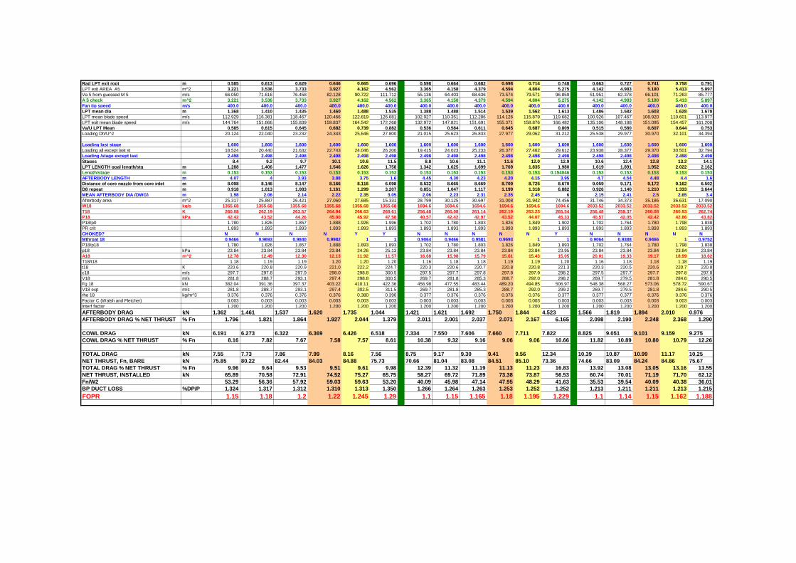
Rad LPT exit root m 0.585 0.613 0.629 0.646 0.665 0.696 0.598 0.664 0.682 0.698 0.714 0.748 0.663 0.727 0.741 0.758 0.791
LPT exit AREA A5 m^2 3.221 3.536 3.733 3.927 4.162 4.562 3.365 4.158 4.379 4.594 4.804 5.275 4.142 4.983 5.180 5.413 5.897
Va 5 from guessed M 5 m/s 66.050 71.616 76.458 82.128 90.722 111.712 55.136 64.403 68.636 73.574 79.571 96.859 51.951 62.378 66.101 71.263 85.777
A 5 check m^2 3.221 3.536 3.733 3.927 4.162 4.562 3.365 4.158 4.379 4.594 4.804 5.275 4.142 4.983 5.180 5.413 5.897
Fan tip speed m/s 400.0 400.0 400.0 400.0 400.0 400.0 400.0 400.0 400.0 400.0 400.0 400.0 400.0 400.0 400.0 400.0 400.0
LPT mean dia m 1.368 1.410 1.435 1.460 1.488 1.535 1.388 1.488 1.514 1.539 1.562 1.613 1.486 1.582 1.603 1.628 1.678
LPT mean blade speed m/s 112.929 116.381 118.467 120.466 122.819 126.681 102.927 110.351 112.286 114.126 115.879 119.682 100.926 107.467 108.920 110.601 113.977
LPT exit mean blade speed m/s 144.764 151.666 155.839 159.837 164.542 172.268 132.972 147.821 151.691 155.371 158.876 166.482 135.106 148.188 151.095 154.457 161.208
Va/U LPT Mean 0.585 0.615 0.645 0.682 0.739 0.882 0.536 0.584 0.611 0.645 0.687 0.809 0.515 0.580 0.607 0.644 0.753
Loading Dh/U^2 20.124 22.040 23.232 24.343 25.646 27.800 21.015 25.623 26.833 27.977 29.062 31.212 25.538 29.977 30.970 32.101 34.394
Loading last stage 1.600 1.600 1.600 1.600 1.600 1.600 1.600 1.600 1.600 1.600 1.600 1.600 1.600 1.600 1.600 1.600 1.600
Loading all except last st 18.524 20.440 21.632 22.743 24.046 26.200 19.415 24.023 25.233 26.377 27.462 29.612 23.938 28.377 29.370 30.501 32.794
Loading /stage except last 2.498 2.498 2.498 2.498 2.498 2.498 2.498 2.498 2.498 2.498 2.498 2.498 2.498 2.498 2.498 2.498 2.498
Stages 8.4 9.2 9.7 10.1 10.6 11.5 8.8 10.6 11.1 11.6 12.0 12.9 10.6 12.4 12.8 13.2 14.1
LPT LENGTH goal length/stg m 1.288 1.406 1.477 1.546 1.626 1.758 1.342 1.625 1.699 1.769 1.835 1.980 1.619 1.891 1.952 2.022 2.162
Length/stage m 0.153 0.153 0.153 0.153 0.153 0.153 0.153 0.153 0.153 0.153 0.153 0.154046 0.153 0.153 0.153 0.153 0.153
AFTERBODY LENGTH m 4.07 4 3.93 3.88 3.75 1.6 4.45 4.30 4.23 4.20 4.15 3.95 4.7 4.54 4.48 4.4 1.6
Distance of core nozzle from core inlet m 8.098 8.146 8.147 8.166 8.116 6.098 8.532 8.665 8.669 8.709 8.725 8.670 9.059 9.171 9.172 9.162 6.502
D8 repeat m 0.918 1.013 1.083 1.161 1.299 3.207 0.851 1.047 1.117 1.199 1.318 6.882 0.926 1.140 1.210 1.333 3.644
MEAN AFTERBODY DIA (DWG) m 1.98 2.06 2.14 2.22 2.35 3.05 2.06 2.23 2.31 2.35 2.45 6 2.15 2.41 2.5 2.65 3.4
Afterbody area m^2 25.317 25.887 26.421 27.060 27.685 15.331 28.799 30.125 30.697 31.008 31.942 74.456 31.746 34.373 35.186 36.631 17.090
W18 kg/s 1355.68 1355.68 1355.68 1355.68 1355.68 1355.68 1694.6 1694.6 1694.6 1694.6 1694.6 1694.6 2033.52 2033.52 2033.52 2033.52 2033.52
T18 K 260.08 262.19 263.57 264.94 266.63 269.61 256.48 260.08 261.14 262.19 263.23 265.54 256.48 259.37 260.08 260.93 262.74
P18 kPa 42.42 43.52 44.26 45.00 45.92 47.58 40.57 42.42 42.97 43.52 44.07 45.33 40.57 42.05 42.42 42.86 43.82
P18/p0 1.780 1.826 1.857 1.888 1.926 1.996 1.702 1.780 1.803 1.826 1.849 1.902 1.702 1.764 1.780 1.798 1.838
PR crit 1.893 1.893 1.893 1.893 1.893 1.893 1.893 1.893 1.893 1.893 1.893 1.893 1.893 1.893 1.893 1.893 1.893
CHOKED? N N N N Y Y N N N N N Y N N N N N
Mthroat 18 0.9466 0.9693 0.9840 0.9982 1 1 0.9064 0.9466 0.9581 0.9693 1 1 0.9064 0.9388 0.9466 1 0.9752
P18/p18 1.780 1.826 1.857 1.888 1.893 1.893 1.702 1.780 1.803 1.826 1.849 1.893 1.702 1.764 1.780 1.798 1.838
p18 kPa 23.84 23.84 23.84 23.84 24.26 25.13 23.84 23.84 23.84 23.84 23.84 23.95 23.84 23.84 23.84 23.84 23.84
A18 m^2 12.78 12.49 12.30 12.13 11.92 11.57 16.68 15.98 15.79 15.61 15.43 15.05 20.01 19.33 19.17 18.99 18.62
T18/t18 1.18 1.19 1.19 1.20 1.20 1.20 1.16 1.18 1.18 1.19 1.19 1.20 1.16 1.18 1.18 1.18 1.19
t18 K 220.6 220.8 220.9 221.0 222.2 224.7 220.3 220.6 220.7 220.8 220.8 221.3 220.3 220.5 220.6 220.7 220.8
c18 m/s 297.7 297.8 297.9 298.0 298.8 300.5 297.5 297.7 297.8 297.8 297.9 298.2 297.5 297.7 297.7 297.8 297.8
V18 m/s 281.8 288.7 293.1 297.4 298.8 300.5 269.7 281.8 285.3 288.7 292.0 298.2 269.7 279.5 281.8 284.6 290.5
Fg 18 kN 382.04 391.36 397.37 403.22 410.11 422.36 456.98 477.55 483.44 489.20 494.85 506.97 548.38 568.27 573.06 578.72 590.67
V18 exp m/s 281.8 288.7 293.1 297.4 302.5 311.5 269.7 281.8 285.3 288.7 292.0 299.2 269.7 279.5 281.8 284.6 290.5
rho 18 kg/m^3 0.376 0.376 0.376 0.376 0.380 0.390 0.377 0.376 0.376 0.376 0.376 0.377 0.377 0.377 0.376 0.376 0.376
Factor C (Walsh and Fletcher) 0.003 0.003 0.003 0.003 0.003 0.003 0.003 0.003 0.003 0.003 0.003 0.003 0.003 0.003 0.003 0.003 0.003
Interf factor 1.200 1.200 1.200 1.200 1.200 1.200 1.200 1.200 1.200 1.200 1.200 1.200 1.200 1.200 1.200 1.200 1.200
AFTERBODY DRAG kN 1.362 1.461 1.537 1.620 1.735 1.044 1.421 1.621 1.692 1.750 1.844 4.523 1.566 1.819 1.894 2.010 0.976
AFTERBODY DRAG % NET THRUST % Fn 1.796 1.821 1.864 1.927 2.044 1.379 2.011 2.001 2.037 2.071 2.167 6.165 2.098 2.190 2.248 2.368 1.290
COWL DRAG kN 6.191 6.273 6.322 6.369 6.426 6.518 7.334 7.550 7.606 7.660 7.711 7.822 8.825 9.051 9.101 9.159 9.275
COWL DRAG % NET THRUST % Fn 8.16 7.82 7.67 7.58 7.57 8.61 10.38 9.32 9.16 9.06 9.06 10.66 11.82 10.89 10.80 10.79 12.26
TOTAL DRAG kN 7.55 7.73 7.86 7.99 8.16 7.56 8.75 9.17 9.30 9.41 9.56 12.34 10.39 10.87 10.99 11.17 10.25
NET THRUST, Fn, BARE kN 75.85 80.22 82.44 84.03 84.88 75.73 70.66 81.04 83.08 84.51 85.10 73.36 74.66 83.09 84.24 84.86 75.67
TOTAL DRAG % NET THRUST % Fn 9.96 9.64 9.53 9.51 9.61 9.98 12.39 11.32 11.19 11.13 11.23 16.83 13.92 13.08 13.05 13.16 13.55
NET THRUST, INSTALLED kN 65.89 70.58 72.91 74.52 75.27 65.75 58.27 69.72 71.89 73.38 73.87 56.53 60.74 70.01 71.19 71.70 62.12
Fn/W2 53.29 56.36 57.92 59.03 59.63 53.20 40.09 45.98 47.14 47.95 48.29 41.63 35.53 39.54 40.09 40.38 36.01
BP DUCT LOSS %DP/P 1.324 1.317 1.312 1.310 1.313 1.350 1.266 1.264 1.263 1.253 1.252 1.252 1.213 1.211 1.211 1.213 1.215
FOPR 1.15 1.18 1.2 1.22 1.245 1.29 1.1 1.15 1.165 1.18 1.195 1.229 1.1 1.14 1.15 1.162 1.188

FOPR 1.15 1.18 1.2 1.22 1.245 1.29 1.1 1.15 1.165 1.18 1.195 1.229 1.1 1.14 1.15 1.162 1.188BPR 20 25 30
Fn bare kN 75.850 80.220 82.440 84.030 84.880 75.730 70.660 81.040 83.080 84.510 85.100 73.360 74.660 83.090 84.240 84.860 75.670
LONG COWLLONG COWL LENGTH m 8.908 9.026 9.097 9.164 9.246 9.378 9.574 9.857 9.931 10.000 10.067 10.212 10.627 10.899 10.960 11.030 11.170
LONG COWL AFTERBODY LENGTH m 4.07 4 3.93 3.88 3.75 1.6 4.45 4.3 4.23 4.2 4.15 3.95 4.7 4.54 4.48 4.4 1.6
LONG COWL BYPASS DUCT LENGTH m 4.85 4.97 5.05 5.11 5.20 5.33 5.03 5.30 5.39 5.41 5.49 5.65 5.43 5.70 5.76 5.83 5.97
MAX COWL DIA m 5.35 5.35 5.35 5.35 5.35 5.35 5.89 5.89 5.89 5.89 5.89 5.89 6.39 6.39 6.39 6.39 6.39
AFTERBODY MEAN DIA m 1.98 2.06 2.14 2.22 2.35 3.05 2.06 2.23 2.31 2.35 2.45 6.00 2.15 2.41 2.50 2.65 3.40
COWL DRAG kN 6.19 6.27 6.32 6.37 6.43 6.52 7.33 7.55 7.61 7.66 7.71 7.82 8.82 9.05 9.10 9.16 9.28
COWL DRAG % Fn 8.16 7.82 7.67 7.58 7.57 8.61 10.38 9.32 9.16 9.06 9.06 10.66 11.82 10.89 10.80 10.79 12.26
AFTERBODY DRAG kN 1.36 1.46 1.54 1.62 1.73 1.04 1.42 1.62 1.69 1.75 1.84 4.52 1.57 1.82 1.89 2.01 0.98
AFTERBODY DRAG % Fn 1.80 1.82 1.86 1.93 2.04 1.38 2.01 2.00 2.04 2.07 2.17 6.17 2.10 2.19 2.25 2.37 1.29
TOTAL DRAG kN 7.55 7.73 7.86 7.99 8.16 7.56 8.75 9.17 9.30 9.41 9.56 12.34 10.39 10.87 10.99 11.17 10.25
TOTAL DRAG % Fn 9.96 9.64 9.53 9.51 9.61 9.98 12.39 11.32 11.19 11.13 11.23 16.83 13.92 13.08 13.05 13.16 13.55
BYPASS LOSS %DP/P 1.324 1.317 1.312 1.310 1.313 1.350 1.266 1.264 1.263 1.253 1.252 1.252 1.213 1.211 1.211 1.213 1.215
BYPASS PR LONG COWL 0.9868 0.9868 0.9869 0.9869 0.9869 0.9865 0.9873 0.9874 0.9874 0.9875 0.9875 0.9875 0.9879 0.9879 0.9879 0.9879 0.9878
SHORT COWLSHORT COWL LENGTH = max dia 5.346 5.346 5.346 5.346 5.346 5.346 5.892 5.892 5.892 5.892 5.892 5.892 6.388 6.388 6.388 6.388 6.388
COWL LENGTH REDUCTION m 3.561 3.680 3.751 3.818 3.900 4.032 3.682 3.965 4.038 4.108 4.175 4.320 4.239 4.511 4.572 4.642 4.782
BYPASS DUCT LENGTH m 1.289 1.290 1.294 1.292 1.300 1.298 1.348 1.330 1.349 1.304 1.315 1.330 1.191 1.189 1.186 1.188 1.190
AFTERBODY LENGTH m 7.631 7.680 7.681 7.698 7.650 5.632 8.132 8.265 8.268 8.308 8.325 8.270 8.939 9.051 9.052 9.042 6.382
COWL DRAG kN 3.715 3.715 3.715 3.715 3.715 3.715 4.513 4.513 4.513 4.513 4.513 4.513 5.305 5.305 5.305 5.305 5.305
COWL DRAG % Fn 4.898 4.632 4.507 4.422 4.377 4.906 6.387 5.569 5.432 5.341 5.304 6.152 7.105 6.384 6.297 6.251 7.010
BYPASS LOSS % DP/P 0.352 0.342 0.337 0.331 0.328 0.329 0.339 0.318 0.316 0.302 0.300 0.295 0.266 0.253 0.249 0.247 0.242
AFTERBODY MEAN DIA 1.1 * LONG 2.178 2.266 2.354 2.442 2.585 3.355 2.266 2.453 2.541 2.585 2.695 6.6 2.365 2.651 2.75 2.915 3.74
AFTERBODY DRAG kN 2.81 3.09 3.30 3.53 3.89 4.04 2.86 3.43 3.64 3.81 4.07 10.42 3.28 3.99 4.21 4.54 4.28
AFTERBODY DRAG % Fn 3.70 3.85 4.01 4.21 4.59 5.34 4.04 4.23 4.38 4.51 4.78 14.20 4.39 4.80 5.00 5.35 5.66
TOTAL COWL DRAG kN 6.53 6.80 7.02 7.25 7.61 7.76 7.37 7.94 8.15 8.32 8.58 14.93 8.58 9.29 9.51 9.85 9.59
TOTAL COWL DRAG % Fn 8.60 8.48 8.51 8.63 8.96 10.24 10.43 9.80 9.81 9.85 10.08 20.35 11.49 11.19 11.29 11.60 12.67
D BYPASS LOSS % DP/P 0.972 0.975 0.976 0.979 0.985 1.021 0.927 0.947 0.947 0.951 0.952 0.958 0.947 0.959 0.962 0.966 0.973
SHORT COWL BYPASS P.R. 0.9965 0.9966 0.9966 0.9967 0.9967 0.9967 0.9966 0.9968 0.9968 0.9970 0.9970 0.9971 0.9973 0.9975 0.9975 0.9975 0.9976
Fn/W2 53.29 56.36 57.92 59.03 59.63 53.20 40.09 45.98 47.14 47.95 48.29 41.63 35.53 39.54 40.09 40.38 36.01

APPENDIX 7 SHEET 9 PAGE 237 INSTALLATION DESIGN AND LOSSES OPEN ROTORS
CRUISE ONLY BPR 30 50 80
AFTERBODY
D LPT TIP out m 1.697 1.820 1.826
LPT EXIT AREA to CENTRE m^2 2.262 2.601 2.618
Rad LPT TIP out m 0.849 0.910 0.913
ADD RAD TO CLEAR LPT m 0.100 0.100 0.100
Afterbody rad over LPT TE m 0.949 1.010 1.013
Afterbody dia over LPT TE m 1.897 2.020 2.026
A8 m^2 1.295 1.308 1.333
LPT exit h/t 0.500 0.500 0.500
A LPT OUT m^2 1.697 1.951 1.964
D8 m 1.284 1.290 1.303
LPT Tin 46 K 952.79 950.51 949.20
LPT Tout 49 K 655.70 654.73 652.76
ASSUMPTIONS Strut behind LPT adds 0.25 m length LPT DEL T C 297.09 295.78 296.44
No bypass duct LPT MEAN T K 804.25 802.62 800.98
Bypass ratios at cruise Gear ratio supplied LPT MEAN T / 1000 0.804 0.803 0.801
Afterbody boat-tail angle 14deg as turbofan LPT stage loading constant - adds or reduces stage numbers 20 W LPT MEAN (W 48) kg/s 65.89 65.89 65.89
Angle of duct to core entry 10 deg Afterbody length allows LPT reduced length and fan closer to core Fuel flow rate kg/s 1.1866 1.1866 1.1866
Nose cone angle 27.5 deg far LPT mean 0.0183 0.0183 0.0183
PROPELLER - CRUISE BPR 30 50 80 Cp mean J/kg.K 1129.8 1129.4 1129.0
PROP OUTER PRESSURE RATIO 1.13 1.077 1.048 T 5 K 655.59 654.63 652.68
BYPASS "Nozzle area" m^2 19.202 33.507 55.1 T / 1000 0.65559 0.65463 0.65268
PROP ISENTROPIC EFFY 0.8345 0.8357 0.8363 far 5 0.0181 0.0181 0.0181
PROP INNER PRESSURE RATIO 1.084 1.051 1.032 Cp 5 J/kg.K 1090.8 1090.5 1090.0
Alt km 10.67 10.67 10.67 γ/(γ-1) 5 3.801 3.800 3.798
Mach 0.83 0.83 0.83 γ 5 1.357 1.357 1.357
pamb kPa 23.835 23.835 23.835 30 Mach LPT out 5 GOAL SEEK 0.481 0.405 0.407
tamb K 218.8 218.8 218.8 T/t 5 1.041 1.029 1.030
T0 K 248.94 248.94 248.94 t 5 K 629.6 636.0 633.9
P0 kPa 37.447 37.447 37.447 P 5 kPa 34.729 34.502 34.047
Axial Mach into prop 0.830 0.830 0.830 P/p 5 1.166 1.116 1.117
T2/t2 1.138 1.138 1.138 p 5 kPa 29.785 30.924 30.473
t2 K 218.8 218.8 218.8 rho 5 kg/m^3 0.1648 0.1694 0.1675
P2/p2 1.571 1.571 1.571 W 5 kg/s 66.571 66.571 66.571
p2 kPa 23.835 23.835 23.835 c5 m/s 495.2 497.7 496.9
rho 2 kg/m^3 0.380 0.380 0.380 Rad LPT exit root m 0.424 0.455 0.456
c2 m/s 296.5 296.5 296.5 40 LPT exit AREA A5 m^2 1.697 1.951 1.964
V2 m/s 246.1 246.1 246.1 Va 5 from guessed M 5 m/s 238.0 201.4 202.4
BPR 30 50 80 A 5 check m^2 1.697 1.951 1.964
W2 kg/s 2101.3 3457.0 5490.5 Fan tip speed m/s 250.0 250.0 250.0
A2 in m^2 22.50 37.01 58.78 Gear ratio 3.75 4.15 5.2
h2 in 0.25 0.25 0.25 LPT mean dia m 1.128 1.174 1.176
Atip in m^2 23.995 39.476 62.698 LPT mean blade speed m/s 191.265 171.754 171.100
Dtip in m 5.527 7.090 8.935
Fan eta poly 0.8374 0.8374 0.8374 LPT exit mean blade speed m/s 215.9 199.7 199.2
Dtip out/ Dtip in 0.950 0.960 0.966 Va/U LPT Mean 1.244 1.173 1.183
Dtip out m 5.251 6.807 8.632 50 Loading Dh/U^2 9.175 11.324 11.432
Atip out m^2 21.656 36.388 58.519 Loading last stage 1.600 1.600 1.600
FPR 1.13 1.077 1.048 Loading all except last st 7.575 9.724 9.832
T13 K 259.57 255.34 252.97 Loading /stage except last 2.498 2.498 2.498
P13/po 1.7753 1.6921 1.6465 Stages 4.03 4.89 4.94
T13/t13 1.178 1.162 1.153 Dia at LPT entry, tip m 1.123 1.123 1.123
t13 K 220.272 219.680 219.347 FAN RPM 863.8 673.5 534.4
Mach 13 0.9445 0.9009 0.8755 LPT LENGTH goal length/stg m 0.616 0.747 0.754
P13 kPa 42.315 40.330 39.244 Length/stage m 0.153 0.153 0.153
rho 13 kg/m^3 0.377 0.378 0.379 AFTERBODY LENGTH m 8.80 9.00 9.20
c13 m/s 297.50 297.10 296.87 60 Splitter Diameter - repeat m 2.053 2.183 2.329
V13 m/s 280.979 267.658 259.902 Cowl diameter over LPT TE (repeat) m 1.897 2.020 2.026
W13 kg/s 2033.5 3389.2 5422.7 NACELLE/FAN DIA RATIO 0.371 0.308 0.261
A fan exit m^2 19.20 33.49 55.11 D8 repeat m 1.284 1.290 1.303
GASTURB A18 m^2 19.202 33.51 55.13 MEAN AFTERBODY DIA (DWG) m 2.0 2.0 2.0
A fan root out m^2 2.460 2.893 3.412 Afterbody area m^2 55.292 56.549 57.805
Droot fan exit m 1.770 1.919 2.084 W18 kg/s 2033.5 3389.2 5422.7
h/t fan out 0.320 0.271 0.233 T18 K 259.6 255.3 253.0
Acore m^2 0.850 0.850 0.850 P18 kPa 42.32 40.33 39.24
Asplitter m^2 3.31 3.74 4.26 V18 exp m/s 280.98 267.66 259.90
Dsplitter m 2.053 2.183 2.329 70 rho 18 kg/m^3 0.377 0.378 0.379
Droot in fan entry m 1.382 1.772 2.234 Factor C (Walsh and Fletcher) 0.003 0.003 0.003
Fan RPM cruise 863.8 673.5 534.4 Interf factor 1.200 1.200 1.200
AFTERBODY DRAG kN 2.962 2.757 2.661
AT 70% BLADE SPAN
Dia m 4.284 5.494 6.924 THRUST ASSESSMENT
Blade speed m/s 193.75 193.75 193.75 Del T outer K 10.63 6.40 4.03
Advance ratio at 0.7D 4.418 4.418 4.418 Cp kJ/kg.K 1.00 1.00 1.00
DVw m/s 54.865 33.032 20.800 Power outer kW 21616.3 21690.9 21853.6
Tan swirl 0.196 0.124 0.080 V0 repeat m/s 246.1 246.1 246.1
Swirl at 70% span deg 11.08 7.06 4.59 80 Propfan efficiency to match Gasturb 0.787 0.800 0.803
cos swirl 0.981 0.992 0.997 Net Thrust of bypass air from prop effy kN 69.14 70.50 71.34
Incident vel at 0.7D m/s 313.21 313.21 313.21 Core nozzle Mach No (Gasturb) 0.7618 0.7549 0.7405
Incident Mach at 0.7D 1.056 1.056 1.056 Gross thrust of core kN 25.11 25.01 24.50
u - DVw m/s 138.89 160.72 172.95 Core inlet airflow kg/s 67.78 67.78 67.78
Vrel off rotor m/s 282.58 293.93 300.79 Mom drag of core air kN 16.681 16.681 16.681
De Haller at 0.7D 0.90 0.94 0.96 Net thrust of core kN 8.433 8.330 7.816
RPS - revs per second n 14.40 11.22 8.91 Total Fn, bare with offtakes, calculated kN 77.570 78.830 79.160
Power input to prop (outer) kW 21616.3 21690.9 21853.6 Total Fn, bare with offtakes, Gasturb kN 77.57 78.83 79.16
Power input to prop SHP 28976.3 29076.2 29294.3 SFC BARE, calculated 15.297 15.053 14.990
AT BLADE TIP 90 GASTURB SFC BARE 15.297 15.053 14.990
Blade speed m/s 250.0 250.0 250.0 Installed Fn CALC 74.608 76.073 76.499
Advance ratio at tip 3.093 3.093 3.093 Installed Fn, Gasturb 74.608 76.073 76.499
Incident vel at tip m/s 350.80 350.80 350.80 Installed SFC CALC and Gasturb 15.90 15.60 15.51Incident Mach at tip 1.183 1.183 1.183
COMPARISON WITH PROPFAN TEST DATA
Power loading kW/m^2 784.0 468.2 293.3 ROHRBACH PROPFAN ETA 0.765 0.755 0.775
Power loading 50 max per stage? SHP/D^2 97.63 58.30 36.53 BYPASS NET THRUST WITH ROHRBACH ETA 67.19 66.55 68.82
Aspect ratio 5 5.5 6 TOTAL BARE Fn WITH ROHRBACH ETA 75.63 74.88 76.64
Mean chord m 0.41 0.48 0.56 INSTALLED Fn 72.67 72.12 73.98
Activity factor 235 max? 116.73 106.12 97.27 100 SFC INST WITH ROHRBACH FAN 16.33 16.45 16.04Power coefficient 1.7 OK 3.70 2.26 1.43 SFC ROHRBACH / SFC GASTURB 1.027 1.055 1.034
STAGES 2 2 1 GASTURB ETA - ROHRBACH ETA % 2.211 4.486 2.842
Power coefficient per stage 1.85 1.13 1.43
Thrust coeff 0.94 0.58 0.37 "JET" VELOCITIES
Vcore FE m/s 377.3 375.7 368.0
V18 / VcoreFE 0.745 0.712 0.706
Vb from thrust 18 m/s 280.10 266.90 259.25
VB/VE from thrust 0.742 0.710 0.705
Vbthrust/Vbpressure 0.997 0.997 0.998
Page 237
2
L
13
18

238
APPENDIX 8 INSTALLATION DIMENSIONS SUMMARY Text reference 3.1.12.11 Dimensions in metres
TABLE A8.1 INSTALLATION DIMENSIONS BPR 5.98 10 15 20 25 30 FAN TIP DIAMETER
2.794 3.505 4.230 4.846 5.392 5.888
FAN PRESSURE RATIO
1.795 1.5 1.33 1.245 1.195 1.162
BYPASS NOZZLE DIAMETER
2.74 3.48 4.23 4.87 5.43 5.94
CORE NOZZLE DIAMETER
1.10 1.22 1.27 1.30 1.32 1.33
LPT OUTLET DIAMETER
1.85 2.15 2.43 2.66 2.86 3.03
LPT STAGES 5.0 7.1 9.1 10.6 12.0 13.2 LPT LENGTH 0.765 1.089 1.385 1.626 1.835 2.022 MAXIMUM COWL DAIMETER
3.294 4.006 4.730 5.346 5.892 6.388
LONG COWL
COWL LENGTH
5.396 6.904 8.211 9.246 10.067 11.030
AFTERBODY LENGTH
2.25 2.65 3.32 3.75 4.15 4.40
SHORT COWL
COWL LENGTH
3.294 4.005 4.730 5.346 5.892 6.388
AFTERBODY LENGTH
4.35 5.55 6.80 7.650 8.325 9.042

APPENDIX 9
SUMMARY OF LONG AND SHORT COWL INSTALLED CRUISE PERFORMANCE
PAGE
239 SHEET 1 THIS FRONT SHEET
240 SHEET 2 LONG COWL, BPR 6, 10, 15
241 SHEET 3 LONG COWL, BPR 20, 25, 30
242 SHEET 4 SHORT COWL, BPR 6, 10, 15
243 SHEET 5 SHORT COWL, BPR 20, 25, 30
The results show how the installation losses affect cruise design thrust and SFC.
TEXT REFERENCE SECTION 3.1.13
239

APPENDIX 10
PERFORMANCE EXCHANGE RATES AT CRUISE
TEXT REFERENCE SECTION 3.1.14
0.83 MACH 10670m ISA
All efficiencies isentropic
BPR 5.98 Datum CHANGE Δ SFC % Δ THRUST %
FOPR 1.795 Fan tip efficiency 0.9076 1% eta -0.453 0.461
Fan root efficiency 0.8885 1% eta -0.069 0.171
IPC efficiency 0.8665 1% eta -0.298 0.757
HPC efficiency 0.8606 1% eta -0.273 0.665
Comb PR 0.9597 1% PR -0.303 0.309
HPT efficiency 0.85 1% eta -0.375 0.382
IPT efficiency 0.8748 1% eta -0.302 0.303
LPT efficiency 0.8893 1% eta -0.601 0.612
Bypass loss 0.98492 -1% -0.819 0.830
Core thrust coefficient 0.999 -1% 0.442 -0.435
Bypass thrust coefficient 0.999 -1% 1.718 -1.686
HPT Cooling air % 4.4 -0.01 -0.060 1.297
BPR 20 Datum CHANGE Δ SFC % Δ THRUST %
FOPR 1.245 Fan tip efficiency 0.9122 1% eta -0.749 0.760
Fan root efficiency 0.8885 1% eta -0.109 0.206
IPC efficiency 0.8665 1% eta -0.468 0.925
HPC efficiency 0.8606 1% eta -0.424 0.819
Comb PR 0.9597 1% PR -0.374 0.377
HPT efficiency 0.85 1% eta -0.463 0.466
IPT efficiency 0.8748 1% eta -0.373 0.377
LPT efficiency 0.8942 1% eta -0.915 0.931
Bypass loss 0.98492 -1% -3.254 3.359
Core thrust coefficient 0.999 -1% 0.304 -0.306
Bypass thrust coefficient 0.999 -1% 5.009 -4.774
HPT Cooling air % 4.4 -0.01 -0.336 1.579
KEY
eta isentropic efficiency
PR pressure ratio
244

245
APPENDIX 11 V2527-A5 ENGINE PERFORMANCE MODEL The performance model is discussed in Section 4.2.1. More details are given in this Appendix. Data are shown in TABLE A11.1 below at the take-off flight condition for which there is public data - mainly from Jane’s “Aero Engines” [3.9].
TABLE A11.1 V2527-A5 ENGINE PERFORMANCE MODEL
PUBLIC DATA
V2527-A5 MODEL
DIFFERENCE %
TAKE –OFF, SLS ISA +10oC THRUST kN 117.8 117.8 0
BYPASS RATIO 4.8 4.8 0
FAN PRESSURE RATIO 1.7 1.7 0
OVERALL PRESSURE RATIO VARIOUS 28.5 -
ASSUMED VALUES OF KEY PARAMETERS
INLET AIRFLOW RATE kg/s 355.6
TURBINE ENTRY TEMP (TET) K 1472
FAN INNER PRESSURE RATIO 1.5
BOOSTER PRESSURE RATIO 2.0
HP COMPRESSOR PR 9.5
The GasTurb [3.8] output below (FIG A11.1) gives full details of the take-off point modelled. The efficiencies and cooling flows are round numbers but are sensible modern values. The closeness of the match between the model performance and the public data gives good confidence that the turbine entry temperatures, efficiencies and losses assumed are on average about the right level.
FIG A11.1 V2527-A5 TURBOFAN TAKE-OFF PERFORMANCE MODEL

246
APPENDIX 12
PERFORMANCE EFFECTS OF GAS PROPERTY CHANGES
A12.1 INTRODUCTION This Appendix is essentially Appendix 3 of Ref [5.1]. It is wholly researched, calculated and written by the author of this thesis. Its purpose is to determine the performance effects of changing the working fluid from air to CO2 in a compressor stage, a turbine stage and a single shaft synchronous gas turbine. The subject is discussed further in Section 5.5.8.
The effects of changing either the working fluid or the fuel in a gas turbine are to change the performance of the components and thus the overall performance of the engine. The performance of each component is of course a function of the properties of the gases passing through it, namely the Gas Constant and the Specific Heats at constant pressure and constant volume. These properties vary significantly between gases. Furthermore the specific heats, Cp and Cv, vary for a given gas as a function of temperature. Also, adding small amounts of other gases such as combustion products to a given gas can also affect the gas constant, R. For the Options discussed in Chapter 5 of this thesis, the largest effect on the whole engine is in Option 3, which has CO2 as the working fluid; the fuel is natural gas and enough oxygen injected to ensure complete
combustion of the fuel. Typical rounded values of R, Cp and for air and CO2 are as follows.
TABLE A12.1 GAS PROPERTIES (ROUNDED)
Gases at 288K AIR CO2
GAS CONSTANT, kJ/kg.K R 288 189
SPECIFIC HEAT AT CONSTANT PRESSURE, kJ/kg.K
Cp 1011 834
RATIO OF SPECIFIC HEATS Cp / Cv.
1.40 1.29
Gases at 1550K
AIR + NATURAL GAS COMBUSTION
PRODUCTS (FAR 0.0229)
CO2 + NATURAL GAS + OXYGEN COMBUSTION
PRODUCTS (FAR 0.0243)
GAS CONSTANT, kJ/kg.K R 293 202
SPECIFIC HEAT AT CONSTANT PRESSURE, KJ/kg.K
Cp 1305 1390
RATIO OF SPECIFIC HEATS Cp / Cv.
1.29 1.17

247
In order to illustrate the effects of changing the gases in a gas turbine, three examples (compressor stage, turbine stage and whole engine) will be summarised, with some explanations. The gases of Option 3 are taken for all 3 examples (natural gas fuel with O2 oxidant and CO2 working fluid) and compared with the same engine breathing air and using natural gas fuel. Section A.12.1. A typical compressor stage Section A.12.2. A typical high pressure turbine stage Section A.12.3. A typical whole engine A12.2 EFFECTS OF CHANGE IN WORKING FLUID FOR A TYPICAL COMPRESSOR STAGE A typical compressor stage (to suit the Modern Reference Engine) is now taken as an example to demonstrate the effects of switching the working fluid from air to CO2. The stage is designed for air and then operated with CO2. The design has been done for the “mean line” of the compressor, that is the line joining the mid height points of the blades. The physical dimensions of the blading and the annulus have been kept unchanged when the working fluid is switched from air to CO2.
The operating point with CO2 has the same inlet flow Mach number as the air design point. It also has a rotational speed such that the incidence on the rotor is the same as for the air design point. This means the blade Mach number is very close to the same value as for the air design point, and thus represents the same non-dimensional speed as the air design point. The purpose of the calculations is
STATOR
BLADE
FIG A12.1 DIAGRAM OF COMPRESSOR STAGE
ROTOR
AIR

248
to investigate whether the pressure ratio and efficiency of the compressor stage change when it operates on CO2 rather than air, at the same non-dimensional speed and inlet Mach number. Results are shown in TABLE A12.2 below.
TABLE A12.2 COMPRESSOR OPERATION
AIR CO2
Inlet pressure kPa 101.33 101.33
Inlet temperature K 288.15 288.15
Inlet flow Mach Number 0.6 0.6
Inlet area sq. metres 3.071 3.071
Inlet flow rate kg / sec 622.0 744.1
Inlet flow density kg/cu. metre
1.025 1.562
Blade speed metres / sec 304.8 239.5
Rotational speed rpm 100% 78.6%
Rotor incidence degrees 0.0 0.0
Rotor inlet dynamic head kPa 90.8 85.9
Rotor loss / dynamic head % 4.96 4.97
Rotor exit angle degrees 46.24 46.24
Rotor exit annulus area sq. metres 2.614 2.614
Stator incidence degrees 0.0 +0.7
Stator inlet dynamic head kPa 36.27 34.60
Stator loss / dynamic head % 4.83 4.83
Stator exit angle degrees 0.0 0.0
Stator exit annulus area sq. metres 2.486 2.486
Stator outlet Mach Number 0.5472 0.5470
RESULTS
MASS FLOW RATE kg / sec 622.0 744.1
PRESSURE RATIO 1.379 1.364
EFFICIENCY (polytropic) % 88.0 88.09
TEMPERATURE RISE K 31.59 23.97
POWER INPUT kW 19860 14865
ROTATIONAL SPEED rpm Datum 78.6%
EXPLANATIONS In the inlet, at fixed Mach number, the ratio of total to static temperature can be found, as can the ratio of total and static pressure. They are functions of gamma
( ).
T / t = 1 + [( - 1)/2] M2
P/p = (T/t)k, where k = /( - 1)

249
Thus at 0.6 Mach number (M), for T = 288.15K, t = 268.85K for air and 273.7K for CO2. Also at 0.6 Mach number, for P = 101.33 kPa, p = 79.45 kPa for air and 80.76 kPa for CO2.
The speed of sound, c, in a gas is c = ( Rt) In the inlet this gives c = 329.2 m/s for air and c = 258.6 m/s for CO2, mainly due to the differences in the Gas Constant, R. So the velocity of the air at the inlet (0.6 Mach number) is 197.5m/s for air and 155.1m/s for CO2, which is 78.6% of the value for air.
The density, , of the inlet air is = p/(Rt).
In the inlet this gives = 1.025 kg/m3 for air and 1.562 kg/m3 for CO2, a 53% increase. Again, the difference is largely due to the difference in the Gas Constant, R.
The mass flow rate is W = Av. In the inlet this gives W = 622.0 kg/s for air and 744.1 kg/s for CO2 (a 20% increase due to 1.52 times higher density and 0.79 times the velocity). Because all the angles of the velocity triangles are geometrically very similar for air
and CO2, the function h/U falls for CO2 by the same amount as all the velocities
(78.6% of the value for air). Thus the work per kg/sec of flow (= h = U x change
in whirl velocity) falls by (0.786)2 = 0.62. The work per kg/sec, h = Cp. T. Thus the temperature rise for air is 31.6 deg and for CO2 is 24.0 deg (0.75 times). This arises because for CO2, the work per kg/sec is 0.62 times and the Cp is 0.82 times the values for air.
The pressure ratio is given by P4/P1 = (T4/T1)n where n = [ / ( -1)] . [1/ ] where is the polytropic efficiency. This gives a pressure ratio of 1.379 for air and 1.364 for CO2 assuming the same efficiency. The efficiency is calculated by taking the same loss for each blade row expressed as a fraction of the dynamic head entering the blade row. This is justified in this case because there is no significant change in incidence on either blade row. This calculation shows that the efficiency of the two cases is virtually identical, the CO2
case being only 0.09% higher efficiency than with air. Thus the assumption of equal efficiencies to calculate the pressure ratios is valid.

250
It is important to note that the exit Mach number is virtually identical in the two cases. This means that subsequent stages in a multi-stage machine will show very similar differences between the air and CO2 operating parameters. A.12.2.1 CONCLUSIONS FOR COMPRESSORS. a) The air based compressor characteristics used for engine calculations can be used for CO2 using the characteristics expressed in the full non-dimensional forms as follows.
FLOW [W T / P ] [ R/ ]
SPEED N / [ ( Rt)] b) The efficiency should be increased by 0.09% polytropic when using CO2. c) The pressure ratio should be scaled down in the ratio 1.364/1.379 = 0.989. A12.3 EFFECTS OF CHANGE OF WORKING FLUID AND FUEL IN A TURBINE. The turbine chosen is a typical first stage of a turbine from a single shaft, 250 MW machine (very like the MRE) of about 17.0 overall pressure ratio and 1550K firing temperature, driving a synchronous electrical generator.
The engine is designed for operation on air and natural gas, and the effects of changing the working fluid to CO2 and the fuel to natural gas with oxygen injection are discussed. The turbine main parameters are listed below for the two cases. Gas properties are given earlier in this Appendix. The turbine is assumed to be
ROTOR BLADE
FIG A12.2 DIAGRAM OF TURBINE STAGE
TURBINE NOZZLE
COMBUSTOR
4 5 6

251
running synchronously in both cases, with the same inlet conditions to facilitate comparison. Results are in the following table (A12.3).
TABLE A12.3 TURBINE OPERATION
AIR CO2
Inlet pressure kPa 1627.8 1627.8
Inlet temperature K 1550 1550
Fuel Natural gas Natural gas
Oxidant Air Oxygen
Fuel to fluid ratio 0.0229 0.0326
Nozzle throat area sq. metres 0.371 0.371
Nozzle throat Mach Number 1.0 1.0
Nozzle exit annulus area sq. metres 0.879 0.879
Nozzle exit gas angle degrees 65.0 65.0
Rotor outlet annulus area sq. metres 1.069 1.069
Rotor inlet hub diameter metres 2.170 2.170
Rotor inlet tip diameter metres 2.414 2.414
Rotor inlet mid height blade angle
degrees 43.7 43.7
Rotor outlet mid height blade angle
degrees -57.0 -57.0
Rotational speed r.p.m. 3000 3000
PERFORMANCE RESULTS
Total gas flow rate kg / sec 598.1 688.1
Outlet total temperature K 1336 1398
Outlet total pressure kPa 802 773
Total power output MW 162.5 144.8
Efficiency % poly 91.0 93.3
Loading ( H)/U2 2.10 1.62
Rotor inlet relative Mach No. 0.584 0.514
Rotor inlet gas angle degrees 43.7 34.8
Rotor outlet gas angle degrees -57.0 -57.0
Rotor inlet dynamic head kPa 214 154
Rotor dynamic head loss 0.246 0.257
Explanations. i) Gas flow. The gas flow rate is a function of the inlet temperature (T) and pressure (P), the throat area (A) and Mach Number (M), and the gas properties.

252
W = A . P . M . . [ 1 + {( - 1)/2}. M2] [- (1 + )/(2{ - 1)]
[ R . T ]
Inserting the gas properties (R and ) and M = 1 gives the results above. As further illustration, the ratio of the flows for the two cases is approximately equal to the following simplified expression (derived from the full one above).
W (CO2) = [ c / a ] . [ Ra / Rc ] approximately W (AIR) Where suffices “a” and “c” refer to air and CO2 respectively. Putting in the numbers from above shows how the flow change arises.
W (CO2) = [ 1.174 / 1.297 ] . [ 292.9 / 206.0 ] W (AIR) = 0.951 x 1.192 = 1.134 approximately (i.e. about 13.4% increase – compares well with the accurate value of 15.0% increase above). The same conclusion can be drawn from consideration of more basic equations, as follows. Density. Density = p / (R . t ) where p and t are the static pressure and temperature respectively. In the case considered, the total pressure and temperature are assumed equal at inlet and so there will be small differences in the static pressure and temperature due to the changes in gas properties. However, it can be easily seen that the ratio of densities at equal pressure and temperature is simply the inverse ratio of the gas constants, Rc and Ra. Thus, assuming equal static pressures and temperatures, since Rc = 206.0 and Ra = 292.9, the density ratio is Density of CO2 = 292.9 / 206.0 = 1.45 Density of Air So, at equal conditions, CO2 is about 42% denser than air.

253
Speed of Sound Speed of sound in a gas, C, is
C = [ . R . t ]. As a simple example, for t = 1300 K, say Speed of sound in AIR, (Mach = 1), Ca = 703 metres / sec Speed of sound in CO2, (Mach = 1), Cc = 560 metres / sec So, at equal temperatures, the throat velocity in a choked turbine will be about 25% faster for air than for CO2. Taking the simple, accurate equation of flow through an area: - W = Density x area x velocity Since the areas are equal in this case, it can be seen that the flow of CO2, with about 42% higher density but 25% lower velocity, will be about 13.5% higher than for air on a mass basis. This also agrees well with the more rigorous approach above.
ii) Efficiency The polytropic efficiency changes when the operating gas changes. If the engine is operating synchronously (as assumed above) the blade speeds will be unaltered. Assuming as above that the turbine is choked, the axial velocity for the CO2 case will be 25% less than for air, leading to a negative incidence on the first rotor of 9 degrees. Turbines are generally able to operate efficiently with this incidence level. A small increase in rotor dynamic head loss has been incorporated to allow for the incidence change, as shown above. (The NGV loss is assumed unchanged for this exercise – a reasonably valid assumption). The efficiency can then be re-computed, and for the case above this actually gives an efficiency increase of about 2.3% despite the slightly increased fraction of dynamic head loss in the rotor. This is because the dynamic head onto the rotor is 28% lower than for air. As a further check, the efficiency change result is very consistent with the Smith Chart [3.14], which correlates efficiency against loading
( H / U2).

254
A.12.3.1 CONCLUSIONS FOR TURBINES a) The turbine may be simulated in the engine calculations by a fixed nozzle
throat area and by adjusting the efficiency. b) The efficiency of the turbine should be adjusted according to changes in the
loading parameter, H /U2, by using the Smith Chart correlation. A12.4 EFFECTS OF CHANGE OF WORKING FLUID AND FUEL IN AN ENGINE To demonstrate the effects of changing an engine from using air to using CO2 as its working fluid, a typical large engine for power generation has been chosen. It has a single shaft connected directly to the generator and runs at a fixed speed of 3000 rpm. It is designed for air and then is operated on CO2 at the same (design) turbine entry temperature (TET) and rotational speed. The effect is that the compressor suffers a gross aerodynamic over-speed. Also, the power is greatly changed. Reference is made to the main body of the report for details of how an engine designed for operating on air must be changed to operate on CO2. A diagram of the engine configuration is shown in Fig. A.12.3 below and results are in TABLE A12.4.
GENERATORTURBINE
COMBUSTOR
EXHAUSTAir
Fuel
COMPRESSOR
23 4
6
FIG A3.3 GAS TURBINE ENGINE - STATION NUMBERING
FIG A12.3 ENGINE STATION DIAGRAM

255
TABLE A12.4 ENGINE OPERATION
Working fluid AIR CO2
Inlet pressure kPa 101.33 101.33
Inlet temperature K 288.15 288.15
Fuel Natural gas Natural gas
Oxidant Air Oxygen
Turbine throat area sq. metres 0.3720 0.3720
Rotational speed rpm 3000 3000
Final nozzle area sq. metres 10.85 10.85
RESULTS
Inlet gas flow rate kg / sec 622 1049
Inlet Mach Number M2 0.60 0.532
Impossible 1.0 !!
Non-dimensional speed N/ RT 8.80 11.31
Inlet non-dimensional flow (W T/P).(R/ ) 1496 2124
Overall pressure ratio P3 / P2 17.0 26.7
Compressor outlet temperature K 696 589
Compressor power MW 262 306
Turbine entry temperature K 1550 1510
Turbine expansion ratio P4 / P6 15.4 23.4
Exhaust total pressure kPa 105.6 113.1
Turbine total power MW 512 816
NET POWER MW 250 509
HEAT RATE Btu/KW.hr 8819 9330
Explanations. The fixed rotational speed results in a large increase in non-dimensional speed (+28%) when changing from air to CO2. Referring to typical compressor characteristics shows that this results automatically in a large increase in the non-dimensional inlet flow rate (typically +30% or more). There is a corresponding increase in the actual flow rate. This is an impossible behaviour for any compressor designed efficiently to operate on air. However, for the purpose of the rest of this demonstration, it is assumed that, with modification, the compressor can deliver this increase in flow. (It would have to have been designed with a quite low inlet Mach number to cope with both air and CO2 or be redesigned for CO2). The next step in this engine calculation is to find the compressor pressure ratio required for the engine to operate at the same TET as for air. This is an iterative procedure, which requires continuity in the turbine nozzle throat area to be satisfied. There is only one solution of pressure ratio for each TET. It is found that there has to be a large increase in the compressor pressure ratio (from 17.0 to 26.7 in this case). This is also an impossible task for a compressor designed efficiently to operate on air. Thus on two counts there must be a change in the

256
compressor when changing from air to CO2. The casings of the engine would also need substantial thickening to accommodate the increase in pressure. The final step is to extract sufficient power from the turbine (by changing the generator demand) such that the exhaust gas flow, the pressure and temperature satisfy continuity for the final nozzle area. The result is that there would be a large increase in the power (nearly doubling) at a TET when changing from air to CO2 if the compressor were modified to accommodate the large aerodynamic over-speed. The heat rate worsens when changing to CO2 because the average cycle temperature at which the fuel is added is lower, giving lower cycle efficiency. A12.4.1 CONCLUSIONS FOR ENGINES There are major changes to the internal and overall performance of an engine if its working fluid is changed from air to carbon dioxide. A new compressor is required, and the turbine performance should be reviewed on a case by case basis.