
CHAPTER 4 ENHANCING VOLTAGE STABILITY AND LOSS...
37
85 CHAPTER 4 ENHANCING VOLTAGE STABILITY AND LOSS MINIMIZATION USING ANN AND PSO WITH UPFC 4.1 INTRODUCTION One of the important operating requirements of a reliable power system is to maintain the voltage to ensure a high quality of customer service. The main reason for the stability problem occurring in the system is due to the sudden increase in load power as well as any fault that occurs in the system. A genetic algorithm is used to optimize the various process parameters involving FACTS devices in a power system. The various parameters taken into consideration are the location of the device, their type and their rated value of the devices as in Nikoukar and Jazaeri (2007). The optimal location and size of SVC device for decreasing voltage stability index, power loss and voltage deviation use PSO and GA for different loading condition as in Kalivani and Kamaraj (2012). An application of Bacterial Foraging (BF) algorithm in optimizing the optimal location and design of Thyristor controlled series capacitor for voltage profile improvement and minimization of losses in a power system utilized the TCSC as the control variable as in Senthilkumar and Renuga (2010). Optimal location and setting of SVC and TCSC devices use Non- dominated Sorting Practical Swarm Optimization (NSPSO) for voltage stability enhancement as in Benabid et al (2009). Power loss minimization
Transcript of CHAPTER 4 ENHANCING VOLTAGE STABILITY AND LOSS...
85
CHAPTER 4
ENHANCING VOLTAGE STABILITY AND LOSS
MINIMIZATION USING ANN AND PSO WITH UPFC
4.1 INTRODUCTION
One of the important operating requirements of a reliable power
system is to maintain the voltage to ensure a high quality of customer service.
The main reason for the stability problem occurring in the system is due to the
sudden increase in load power as well as any fault that occurs in the system. A
genetic algorithm is used to optimize the various process parameters
involving FACTS devices in a power system. The various parameters taken
into consideration are the location of the device, their type and their rated
value of the devices as in Nikoukar and Jazaeri (2007).
The optimal location and size of SVC device for decreasing voltage
stability index, power loss and voltage deviation use PSO and GA for
different loading condition as in Kalivani and Kamaraj (2012). An application
of Bacterial Foraging (BF) algorithm in optimizing the optimal location and
design of Thyristor controlled series capacitor for voltage profile
improvement and minimization of losses in a power system utilized the TCSC
as the control variable as in Senthilkumar and Renuga (2010).
Optimal location and setting of SVC and TCSC devices use Non-
dominated Sorting Practical Swarm Optimization (NSPSO) for voltage
stability enhancement as in Benabid et al (2009). Power loss minimization
86
uses Fuzzy multi-objective formulation and Genetic algorithm using TCSC as
in Bagriyanik et al (2003). Utility of PSO for loss minimization and
enhancement of voltage profile use UPFC as in Kannan and Kayalvizhi
(2011).
PSO techniques for optimal location and parameter setting of TCSC
to improve the power transfer capability, reduce active power losses, improve
stabilities of the power network and decrease the cost of power production
and fulfill the other control requirements by controlling the power flow in
multi-machine power system network as in Rashed et al (2007). PSO based
algorithm uses optimal Automatic Voltage Regulator (AVR) values, On-Line
Tap Changer (OLTC) settings and minimum number of Reactive Power
Compensation Equipment (RPCE). These minimize the real power losses,
with a view to improve the voltage stability of the system as in Ajay-D-
Vimalraj et al (2008).
To maintain the stability of the system, finding the location for
fixing the FACTS controller and also the amount of voltage and angle to be
injected is more important. The hybrid technique includes Artificial Neural
Network and Particle Swarm Optimization. The proposed hybrid method
using MATLAB for different systems such as IEEE 14, 30, 57 and 118 bus
systems has been carried out and the performance evaluation is presented.
4.2 POWER FLOW CALCULATION USING NEWTON-
RAPHSON METHOD
There are different methods available for load flow calculation.
Among them the Newton-Raphson method is the most commonly used
(explained in section, 3.3. By using Newton-Raphson load flow analysis
method, the real and reactive power flow in the bus are calculated using the
Equations (3.6) and (3.7) respectively. Using the equation the real and
87
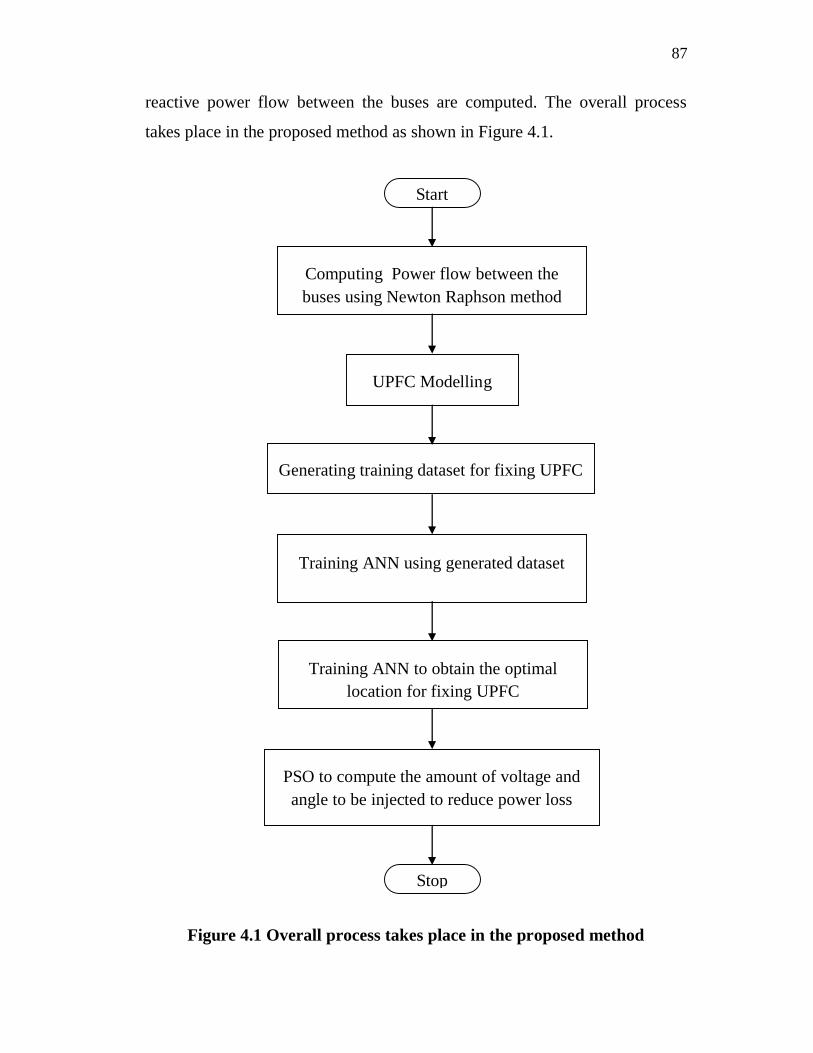
reactive power flow between the buses are computed. The overall process
takes place in the proposed method as shown in Figure 4.1.
Figure 4.1 Overall process takes place in the proposed method
Start
Computing Power flow between the buses using Newton Raphson method
UPFC Modelling
Training ANN using generated dataset
Training ANN to obtain the optimal location for fixing UPFC
PSO to compute the amount of voltage and angle to be injected to reduce power loss
Stop
Generating training dataset for fixing UPFC
88
4.3 UPFC MODELLING
A combination of Static Synchronous Compensator (STATCOM)
and Static Synchronous Series Compensator (SSSC) which are coupled via a
common DC link, allows bidirectional flow of real power between the series
output terminals of the SSSC and the shunt output terminals of the
STATCOM. They are controlled to provide concurrent real and reactive series
line compensation without an external electric energy source. The UPFC, by
means of angularly unconstrained series voltage injection, is able to control,
concurrently or selectively, the transmission line voltage, impedance and
angle or alternatively, the real and reactive power flow in the line. The UPFC
also provides independently controllable shunt reactive compensation. A
detailed explanation is given in section 3.4.
The power injection in terms of voltage and power angle, due to the
insertion of UPFC is given in the Equations (3.8) to (3.11). The amount of
voltage and angle to be injected and the optimal location for fixing UPFC in
the system are identified using the hybrid technique. The next step is
identifying the location for fixing UPFC using artificial neural network.
4.4 ANN TO OBTAIN LOCATION FOR FIXING UPFC
In the proposed method, ANN is used to identify the optimal
location for fixing UPFC to maintain the stability of the system. ANN
consists of two stages: training stage and testing stage. In the training stage,
neural network is trained based on the training dataset and in the testing stage,
if the input variable is given; it gives the corresponding output variables. A
detailed explanation is given in section 3.5.1 and 3.5.2.
89
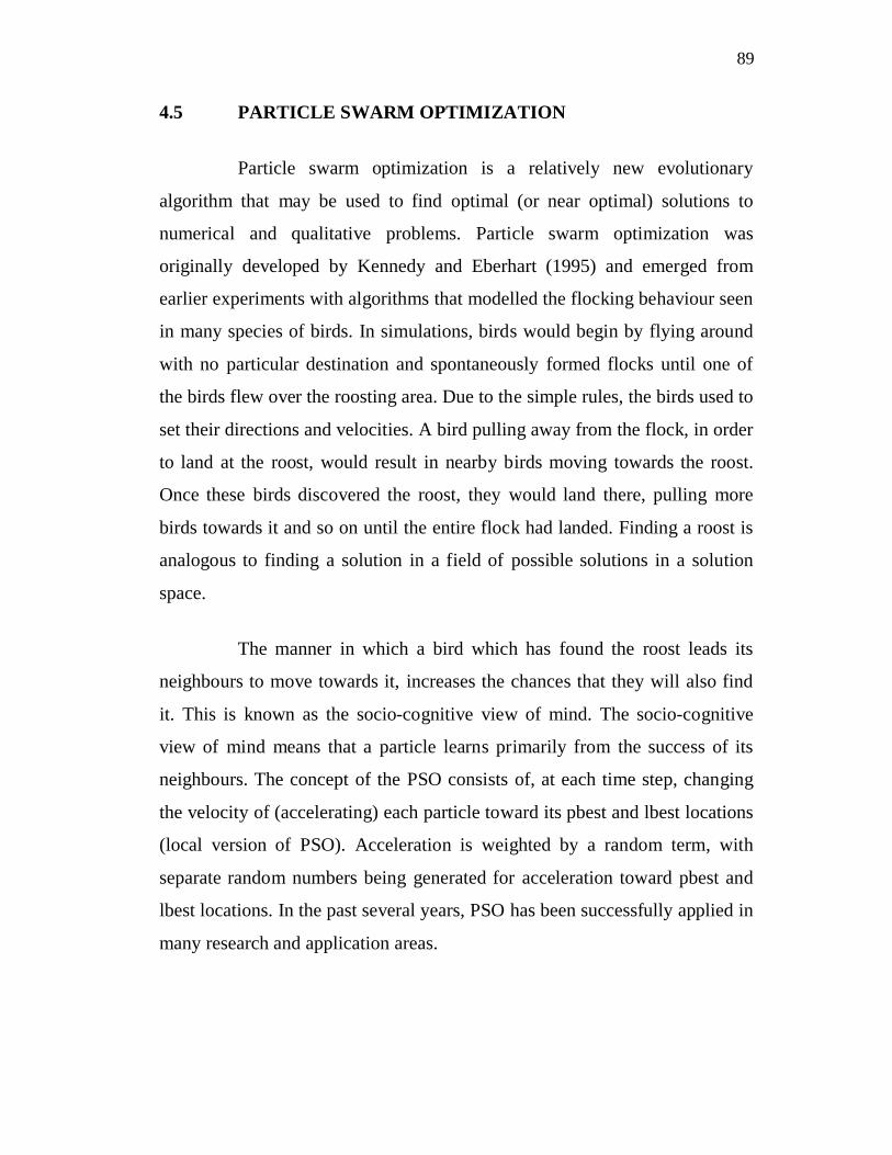
4.5 PARTICLE SWARM OPTIMIZATION
Particle swarm optimization is a relatively new evolutionary
algorithm that may be used to find optimal (or near optimal) solutions to
numerical and qualitative problems. Particle swarm optimization was
originally developed by Kennedy and Eberhart (1995) and emerged from
earlier experiments with algorithms that modelled the flocking behaviour seen
in many species of birds. In simulations, birds would begin by flying around
with no particular destination and spontaneously formed flocks until one of
the birds flew over the roosting area. Due to the simple rules, the birds used to
set their directions and velocities. A bird pulling away from the flock, in order
to land at the roost, would result in nearby birds moving towards the roost.
Once these birds discovered the roost, they would land there, pulling more
birds towards it and so on until the entire flock had landed. Finding a roost is
analogous to finding a solution in a field of possible solutions in a solution
space.
The manner in which a bird which has found the roost leads its
neighbours to move towards it, increases the chances that they will also find
it. This is known as the socio-cognitive view of mind. The socio-cognitive
view of mind means that a particle learns primarily from the success of its
neighbours. The concept of the PSO consists of, at each time step, changing
the velocity of (accelerating) each particle toward its pbest and lbest locations
(local version of PSO). Acceleration is weighted by a random term, with
separate random numbers being generated for acceleration toward pbest and
lbest locations. In the past several years, PSO has been successfully applied in
many research and application areas.
90
4.5.1 Basic Terms used in PSO
The basic terms used in PSO technique are stated and defined as
follows (Abido 2003):
1. Particle X (I): It is a candidate solution represented by a k-dimensional
real-valued vector, where k is the number of optimized parameters. At
iteration i, the jth particle
X (i,j) can be described as:
X i (i ) = [ X j 1 (i ); X j 2 (i );.....X jk (i );.....X jd
where, X’s are the optimized parameters and d represents the number of
control variables
2. Population: It is basically a set of n particles at iteration i.
pop (i )= [ X 1 (i ), X 2 (i ), .........X n (i)]T
where: n represents the number of candidate solutions.
3. Swarm: Swarm may be defined as an apparently disorganized population
of moving particles that tend to cluster together while each particle seems to
be moving in a random direction.
4. Particle velocity V (i): Particle velocity is the velocity of the moving
particles represented by a d-dimensional real valued vector. At iteration i, the
jth particle
Vj (i) can be described as:
V j (i ) = [V j1 (i );V j2 (i );.....V jk (i );.....V jd (i);]

91
where, V jk (i) is the velocity component of the jth particle with respect to the
kth dimension.
5. Inertia weight w (i): It is a control parameter, which is used to control the
impact of the previous velocity on the current velocity. Hence, it influences
the trade-off between the global and local exploration abilities of the particles.
For the initial stages of the search process, large inertia weight to enhance
the global exploration is recommended while it should be reduced at the last
stages for better local exploration. Therefore, the inertia factor decreases
linearly from about 0.9 to 0.4 during a run.
6. Individual best X* (i): As the particles moves through the search space, it
compares its fitness value at the current position to the best fitness value it has
ever reached at any iteration up to the current iteration. The best position that
is associated with the best fitness encountered so far is called the individual
best X* (i).
7. Global best X** (t): Global best is the best position among all the
individual best positions achieved so far.
8. Stopping criteria: Termination of the search process will take place
whenever one of the following criteria is satisfied:
The number of the iterations since the last chance of the best
solution is greater than a pre-specified number.
The number of iterations reaches the maximum allowable
number.
The flow chart of the PSO procedure is shown in Figure 4.2.
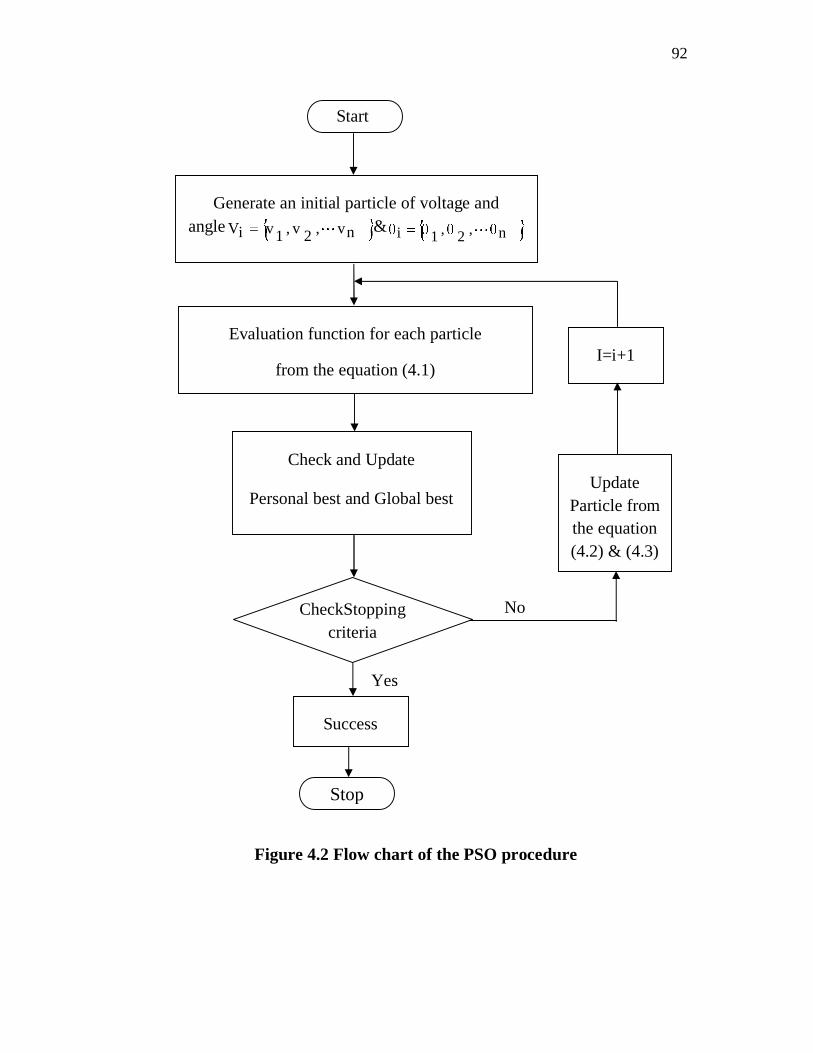
92
Figure 4.2 Flow chart of the PSO procedure
Start
Generate an initial particle of voltage and angle nv,2v,1viV & n,2,1i
Evaluation function for each particle
from the equation (4.1)
Check and Update
Personal best and Global best
Success
Stop
CheckStopping criteria
UpdateParticle from the equation (4.2) & (4.3)
I=i+1
No
Yes
93
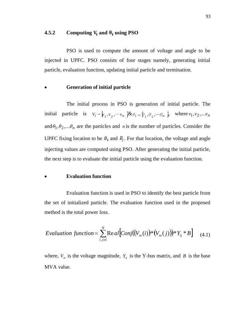
4.5.2 Computing and using PSO
PSO is used to compute the amount of voltage and angle to be
injected in UPFC. PSO consists of four stages namely, generating initial
particle, evaluation function, updating initial particle and termination.
Generation of initial particle
The initial process in PSO is generation of initial particle. The
initial particle is ni vvvV ,, 21& ni ,, 21
, where nvvv ,...., 21
and n,...., 21 are the particles and n is the number of particles. Consider the
UPFC fixing location to be and . For that location, the voltage and angle
injecting values are computed using PSO. After generating the initial particle,
the next step is to evaluate the initial particle using the evaluation function.
Evaluation function
Evaluation function is used in PSO to identify the best particle from
the set of initialized particle. The evaluation function used in the proposed
method is the total power loss.
N
jiijmm BYjViVConjalfunctionEvaluation
1,**)(*)(Re (4.1)
where, mV is the voltage magnitude, ijY is the Y-bus matrix, and B is the base
MVA value.
94
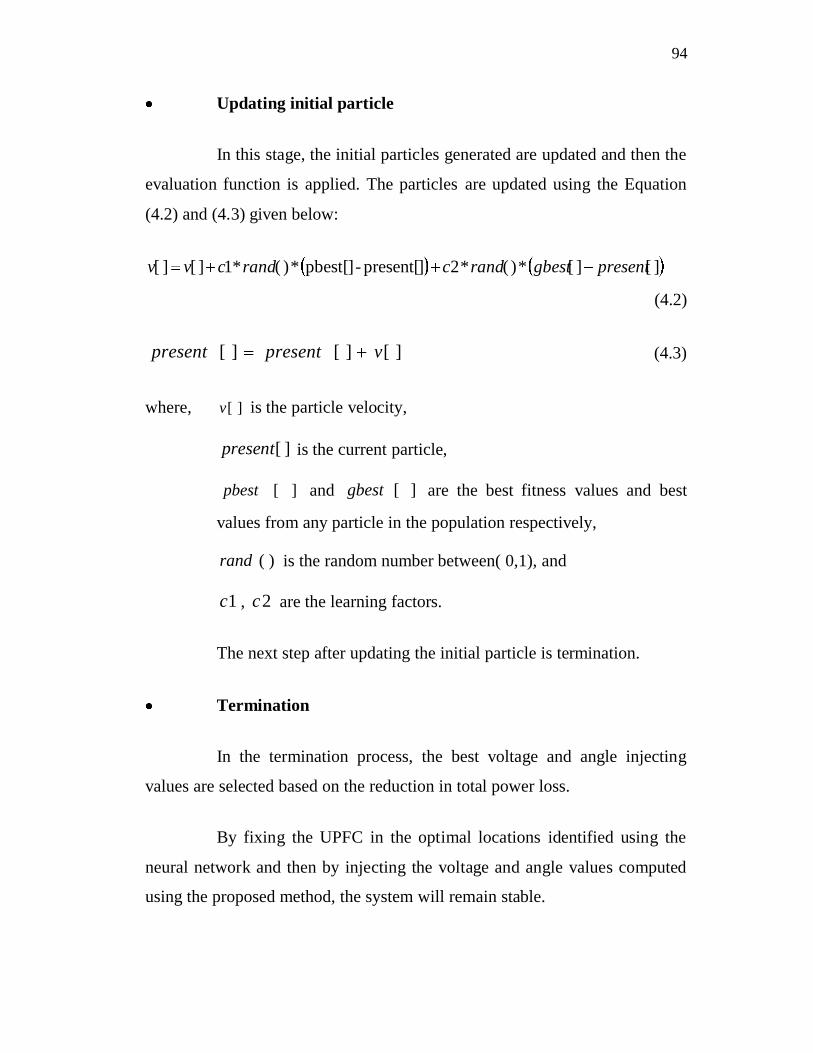
Updating initial particle
In this stage, the initial particles generated are updated and then the
evaluation function is applied. The particles are updated using the Equation
(4.2) and (4.3) given below:
][][*)(*2]present[-]pbest[*)(*1][][ presentgbestrandcrandcvv
(4.2)
][][][ vpresentpresent (4.3)
where, ][v is the particle velocity,
][present is the current particle,
][pbest and ][gbest are the best fitness values and best
values from any particle in the population respectively,
)(rand is the random number between( 0,1), and
1c , 2c are the learning factors.
The next step after updating the initial particle is termination.
Termination
In the termination process, the best voltage and angle injecting
values are selected based on the reduction in total power loss.
By fixing the UPFC in the optimal locations identified using the
neural network and then by injecting the voltage and angle values computed
using the proposed method, the system will remain stable.
95
4.6 SIMULATION RESULTS
The proposed algorithm is applied to IEEE 14, 30, 57 and 118 bus
systems whose data have been given in Appendix 1, 2, 3 and 4. The
simulation studies are done for different scenarios. The first scenario is the
normal operation of conventional NR method. The second scenario is after a
sudden increase power in bus. The third scenario is the one after the UPFC
installed in the proposed method (ANN and PSO). The proposed method is
used to place UPFC in the optimal location to enhance the voltage profile and
reduce the power losses of the system. The simulation parameters considered
for the test cases are shown in Table 4.1.
Table 4.1 PSO parameters
Parameter Chosen Value
Populations size 20
Acceleration coefficients C1 =2.5 and C2 = 1.5
Velocity limits Vmax = 1and Vmin = -1
Inertia weight factor Wmax = 0.9 and Wmin = 0.4
4.6.1 IEEE 14 Bus System
The test system consists of 5 generator buses (bus no. 1, 2, 3, 6 and
8), 9 load buses (bus no. 4, 5, 7, 9, 10, 11, 12, 13 and 14) and 20 transmission
lines. The base MVA considered is 100 MVA. In bus number 5, the optimal
location for connecting UPF using the proposed method is buses 4 and 5. A
comparison of the voltage profile and real power loss of IEEE 14 bus system
for different loading conditions is shown in Figures 4.3 and 4.4 respectively.
96
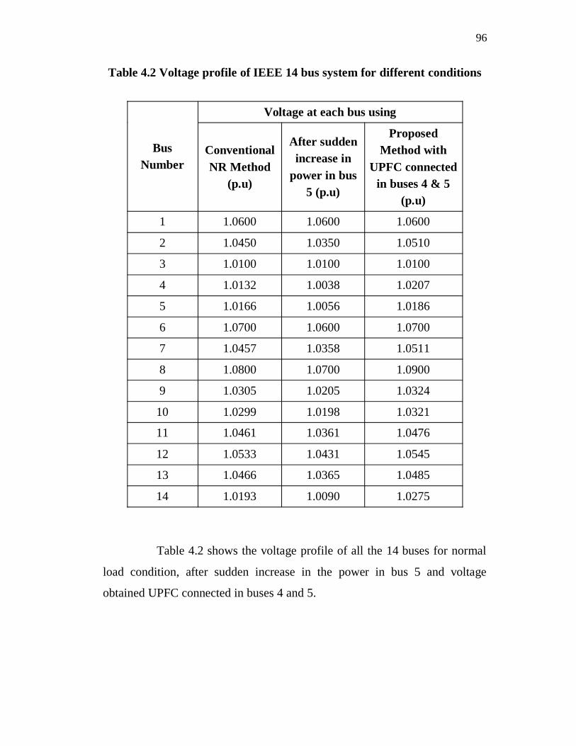
Table 4.2 Voltage profile of IEEE 14 bus system for different conditions
Bus Number
Voltage at each bus using
Conventional NR Method
(p.u)
After sudden increase in
power in bus 5 (p.u)
Proposed Method with
UPFC connected in buses 4 & 5
(p.u)
1 1.0600 1.0600 1.0600
2 1.0450 1.0350 1.0510
3 1.0100 1.0100 1.0100
4 1.0132 1.0038 1.0207
5 1.0166 1.0056 1.0186
6 1.0700 1.0600 1.0700
7 1.0457 1.0358 1.0511
8 1.0800 1.0700 1.0900
9 1.0305 1.0205 1.0324
10 1.0299 1.0198 1.0321
11 1.0461 1.0361 1.0476
12 1.0533 1.0431 1.0545
13 1.0466 1.0365 1.0485
14 1.0193 1.0090 1.0275
Table 4.2 shows the voltage profile of all the 14 buses for normal
load condition, after sudden increase in the power in bus 5 and voltage
obtained UPFC connected in buses 4 and 5.
97
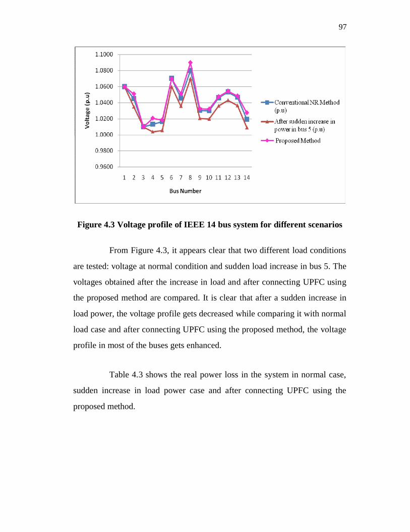
Figure 4.3 Voltage profile of IEEE 14 bus system for different scenarios
From Figure 4.3, it appears clear that two different load conditions
are tested: voltage at normal condition and sudden load increase in bus 5. The
voltages obtained after the increase in load and after connecting UPFC using
the proposed method are compared. It is clear that after a sudden increase in
load power, the voltage profile gets decreased while comparing it with normal
load case and after connecting UPFC using the proposed method, the voltage
profile in most of the buses gets enhanced.
Table 4.3 shows the real power loss in the system in normal case,
sudden increase in load power case and after connecting UPFC using the
proposed method.
98
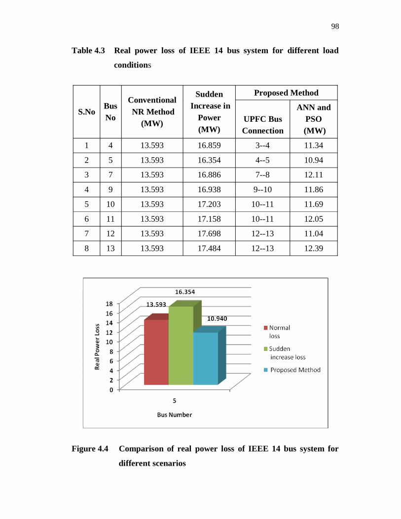
Table 4.3 Real power loss of IEEE 14 bus system for different load
conditions
S.NoBus No
Conventional NR Method
(MW)
Sudden Increase in
Power (MW)
Proposed Method
UPFC Bus Connection
ANN and PSO
(MW)
1 4 13.593 16.859 3--4 11.34
2 5 13.593 16.354 4--5 10.94
3 7 13.593 16.886 7--8 12.11
4 9 13.593 16.938 9--10 11.86
5 10 13.593 17.203 10--11 11.69
6 11 13.593 17.158 10--11 12.05
7 12 13.593 17.698 12--13 11.04
8 13 13.593 17.484 12--13 12.39
Figure 4.4 Comparison of real power loss of IEEE 14 bus system for
different scenarios
99
From Figure 4.4, it is clear that the real power loss occurred for
normal load condition is 13.593 MW. After a sudden increase in the load
power in bus 5, the real power loss is increased to 16.354 MW and then by
using the proposed method with UPFC, the real power loss gets reduced to
10.940 MW.
Table 4.4 Comparison of real power loss of IEEE 14 bus system for the
other methods
Method Real power loss (MW)
Benabid et al (2009) NSPSO 13.460
Bagriyanik et al(2003) GA 12.600
Senthilkumar and Renuga (2010)
BF 12.500
Kannan and Kayalizhi (2011) PSO 11.781
Proposed method ANN with PSO 10.940
It may be seen from Table 4.4, that the proposed method obtains
18.72 % of loss reduction compared to NSPSO value reported in Benabid et al
(2009), 13.17 % of loss reduction compared to GA value mentioned in
Bagriyanik et al (2003), 12.48 % of loss reduction compared to BF value
indicated in Senthilkumar and Renuga (2010) and 7.1 % of loss reduction
compared to BF value referred as in Kannan and Kayalizhi (2011). This
shows the effectiveness of the proposed approach which minimizes the real
power loss compared to the other methods.
4.6.2 IEEE 30 Bus System
The test system consists of 6 generator buses (bus no. 1, 2, 5 ,8,
11,and 13), 24 load buses (bus no. 3, 4, 6, 7, 9, 10, 12, 14 ,15, 16, 17, 18, 19,
20, 21, 22, 23, 24, 25, 26, 27, 28, 29 and 30) and 41 transmission lines. The
base MVA considered is 100 MVA. In bus number 6, the optimal location for
100
connecting UPF using the proposed method is buses 6 and 8. A comparison of
the voltage profile and real power loss of IEEE 30 bus system for different
loading conditions is shown in Figures 4.5 and 4.6 respectively.
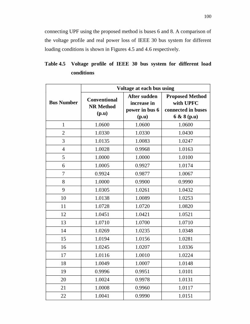
Table 4.5 Voltage profile of IEEE 30 bus system for different load
conditions
Bus Number
Voltage at each bus using
Conventional NR Method
(p.u)
After sudden increase in
power in bus 6 (p.u)
Proposed Method with UPFC
connected in buses 6 & 8 (p.u)
1 1.0600 1.0600 1.06002 1.0330 1.0330 1.04303 1.0135 1.0083 1.02474 1.0028 0.9968 1.01635 1.0000 1.0000 1.01006 1.0005 0.9927 1.01747 0.9924 0.9877 1.00678 1.0000 0.9900 0.99909 1.0305 1.0261 1.0432
10 1.0138 1.0089 1.025311 1.0728 1.0720 1.082012 1.0451 1.0421 1.052113 1.0710 1.0700 1.071014 1.0269 1.0235 1.034815 1.0194 1.0156 1.028116 1.0245 1.0207 1.033617 1.0116 1.0010 1.022418 1.0049 1.0007 1.014819 0.9996 0.9951 1.010120 1.0024 0.9978 1.013121 1.0008 0.9960 1.011722 1.0041 0.9990 1.0151
101
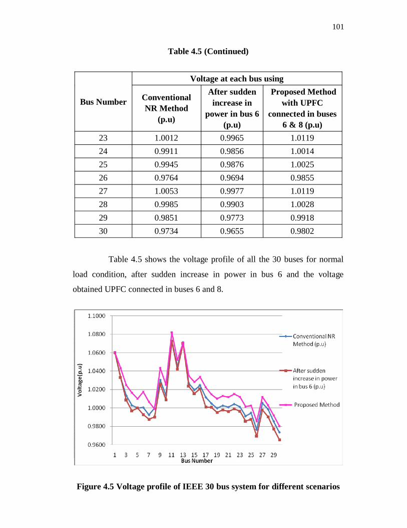
Table 4.5 (Continued)
Bus Number
Voltage at each bus using
Conventional NR Method
(p.u)
After sudden increase in
power in bus 6 (p.u)
Proposed Method with UPFC
connected in buses 6 & 8 (p.u)
23 1.0012 0.9965 1.011924 0.9911 0.9856 1.001425 0.9945 0.9876 1.002526 0.9764 0.9694 0.985527 1.0053 0.9977 1.011928 0.9985 0.9903 1.002829 0.9851 0.9773 0.991830 0.9734 0.9655 0.9802
Table 4.5 shows the voltage profile of all the 30 buses for normal
load condition, after sudden increase in power in bus 6 and the voltage
obtained UPFC connected in buses 6 and 8.
Figure 4.5 Voltage profile of IEEE 30 bus system for different scenarios
102
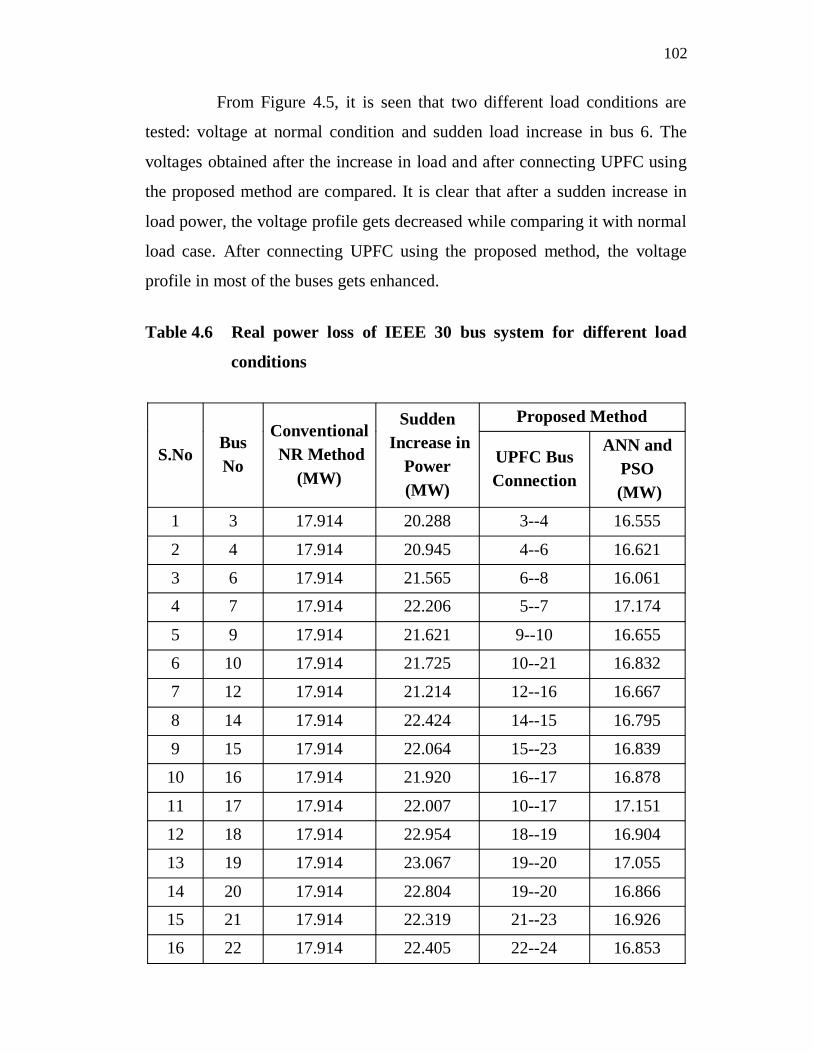
From Figure 4.5, it is seen that two different load conditions are
tested: voltage at normal condition and sudden load increase in bus 6. The
voltages obtained after the increase in load and after connecting UPFC using
the proposed method are compared. It is clear that after a sudden increase in
load power, the voltage profile gets decreased while comparing it with normal
load case. After connecting UPFC using the proposed method, the voltage
profile in most of the buses gets enhanced.
Table 4.6 Real power loss of IEEE 30 bus system for different load
conditions
S.NoBus No
Conventional NR Method
(MW)
Sudden Increase in
Power (MW)
Proposed Method
UPFC Bus Connection
ANN and PSO
(MW) 1 3 17.914 20.288 3--4 16.555
2 4 17.914 20.945 4--6 16.621
3 6 17.914 21.565 6--8 16.0614 7 17.914 22.206 5--7 17.174
5 9 17.914 21.621 9--10 16.655
6 10 17.914 21.725 10--21 16.832
7 12 17.914 21.214 12--16 16.667
8 14 17.914 22.424 14--15 16.795
9 15 17.914 22.064 15--23 16.839
10 16 17.914 21.920 16--17 16.878
11 17 17.914 22.007 10--17 17.151
12 18 17.914 22.954 18--19 16.904
13 19 17.914 23.067 19--20 17.055
14 20 17.914 22.804 19--20 16.86615 21 17.914 22.319 21--23 16.926
16 22 17.914 22.405 22--24 16.853
103
Table 4.6 (Continued)
S.NoBus No
Conventional NR Method
(MW)
Sudden Increase in
Power (MW)
Proposed Method
UPFC Bus Connection
ANN and PSO
(MW) 17 23 17.914 22.357 23--24 16.908
18 24 17.914 22.914 24--25 16.705
19 25 17.914 23.024 25--27 17.198
20 26 17.914 23.034 25--26 17.202
21 27 17.914 22.174 25--27 17.000
22 28 17.914 21.862 8--28 16.843
23 29 17.914 23.053 29--30 17.102
24 30 17.914 23.053 27--30 17.128
Table 4.6 depicts the real power loss in the system in normal case,
sudden increase in load power case and after connecting UPFC using the
proposed method.
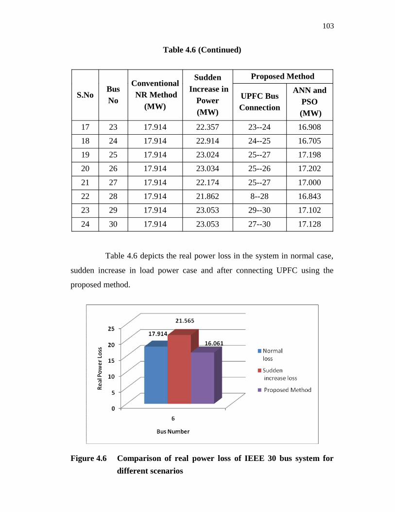
Figure 4.6 Comparison of real power loss of IEEE 30 bus system for different scenarios
104
From Figure 4.6, it is clear that the real power loss that occurred for
normal load condition is 17.914 MW. After a sudden increase in the load
power in bus 6, the real power loss is increased to 21.565 MW and then by
using the proposed method with UPFC, the real power loss gets reduced to
16.061 MW.
Table 4.7 Comparison of real power loss of IEEE 30 bus system for the other methods
Method Real power loss (MW) Nikoukar and Jazaeri (2007) GA 17.695Kalaivani and Kamaraj (2012) PSO 17.543Ajay-D-Vimalraj et al (2008) PSO 16.8264Proposed method ANN with PSO 16.061
Table 4.7 makes it evident that the proposed method obtains 9.23 %
of loss reduction compared to GA value reported in Nikoukar and Jazaeri
(2007), 9.15 % of loss reduction compared to PSO value mentioned in
Kalaivani and Kamaraj (2012) and 4.55 % of loss reduction compared to PSO
value indicated in Ajay-D-Vimalraj et al (2008). This shows the effectiveness
of the proposed approach which minimizes the real power loss compared to
the other methods.
4.6.3 IEEE 57 Bus System
The test system consists of 7 generator buses (bus no. 1, 2, 3, 6, 8,
9, 12) 50 load buses (bus no. 4, 5, 7, 10, 11, 13, 14, 15, 16, 17, 18, 19, 20, 21,
22, 23, 24, 25, 26, 27, 28, 29, 30, 31, 32, 33, 34, 35, 36, 37, 38, 39, 40, 41, 42,
43, 44, 45, 46, 47, 48, 49, 50, 51, 52, 53, 54, 55, 56, 57) and 80 transmission
lines. The base MVA considered is 100 MVA. In bus number 7, the optimal
location for connecting UPF using the proposed method is buses 7 and 8. A
comparison of the voltage profile and real power loss of IEEE 57 bus system
for different loading conditions is shown in Figures 4.7 and 4.8 respectively.
105
Table 4.8 Voltage profile of IEEE 57 bus system for different load conditions
Bus Number
Voltage at each bus using
Conventional NR Method
(p.u)
After sudden increase in
power in bus 7 (p.u)
Proposed Method with UPFC connected in
buses 7 & 8 (p.u)
1 1.0400 1.0400 1.04002 1.0200 1.0200 1.02003 1.0150 1.0150 1.01504 1.0085 1.0085 1.01465 1.0059 1.0058 1.02146 1.0100 1.0100 1.03007 1.0231 1.0207 1.06978 1.0550 1.0550 1.05509 1.0100 1.0100 1.0100
10 1.0052 1.0051 1.005611 0.9980 0.9979 0.998612 1.0250 1.0250 1.025013 0.9977 0.9975 0.998514 0.9891 0.9888 0.990415 1.0070 1.0068 1.007816 1.0207 1.0202 1.020817 1.0213 1.0208 1.021218 1.0065 1.0064 1.012919 0.9814 0.9813 0.988020 0.9782 0.9781 0.984921 1.0275 1.0272 1.034322 1.0295 1.0292 1.036423 1.0281 1.0277 1.035724 1.0179 1.0166 1.038325 0.9725 0.9709 0.991226 0.9786 0.9777 1.000327 1.0115 1.0093 1.046828 1.0301 1.0274 1.069029 1.0457 1.0425 1.0720
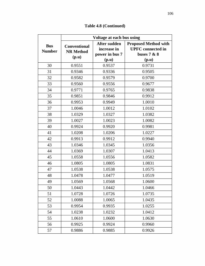
106
Table 4.8 (Continued)
Bus Number
Voltage at each bus using
Conventional NR Method
(p.u)
After sudden increase in
power in bus 7 (p.u)
Proposed Method with UPFC connected in
buses 7 & 8 (p.u)
30 0.9551 0.9537 0.973131 0.9346 0.9336 0.950532 0.9582 0.9579 0.970033 0.9560 0.9556 0.967734 0.9771 0.9765 0.983835 0.9851 0.9846 0.991236 0.9953 0.9949 1.001037 1.0046 1.0012 1.010238 1.0329 1.0327 1.038239 1.0027 1.0023 1.008240 0.9924 0.9920 0.998141 1.0208 1.0206 1.022742 0.9913 0.9912 0.994043 1.0346 1.0345 1.035644 1.0369 1.0307 1.041345 1.0558 1.0556 1.058246 1.0805 1.0805 1.083147 1.0538 1.0538 1.057548 1.0478 1.0477 1.051949 1.0569 1.0568 1.060050 1.0443 1.0442 1.046651 1.0728 1.0726 1.073552 1.0088 1.0065 1.043553 0.9954 0.9935 1.025554 1.0238 1.0232 1.041255 1.0610 1.0600 1.063056 0.9925 0.9924 0.996057 0.9886 0.9885 0.9926
107
Table 4.8 shows the voltage profile of all the 57 buses for normal
load condition, after sudden increase in the power in bus 7 and the voltage
obtained when UPFC is connected in buses 7 and 8.
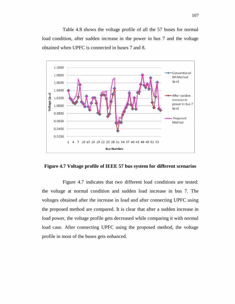
Figure 4.7 Voltage profile of IEEE 57 bus system for different scenarios
Figure 4.7 indicates that two different load conditions are tested:
the voltage at normal condition and sudden load increase in bus 7. The
voltages obtained after the increase in load and after connecting UPFC using
the proposed method are compared. It is clear that after a sudden increase in
load power, the voltage profile gets decreased while comparing it with normal
load case. After connecting UPFC using the proposed method, the voltage
profile in most of the buses gets enhanced.
108
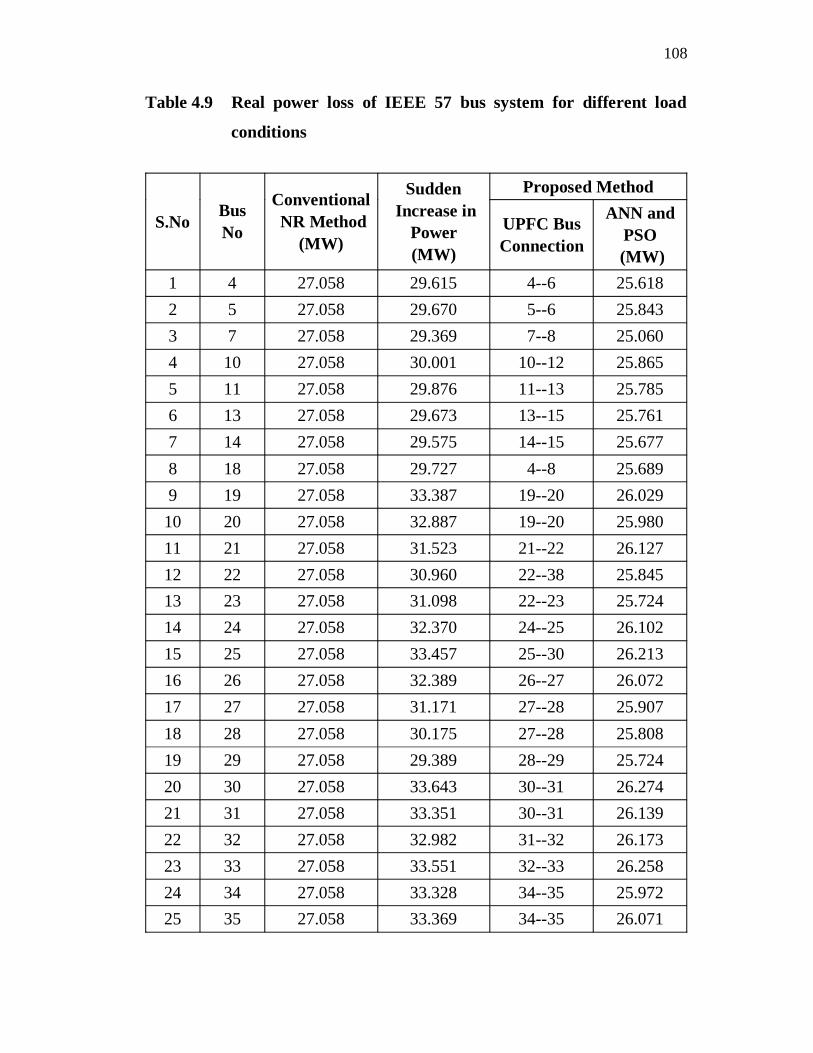
Table 4.9 Real power loss of IEEE 57 bus system for different load
conditions
S.NoBus No
Conventional NR Method
(MW)
Sudden Increase in
Power (MW)
Proposed Method
UPFC Bus Connection
ANN and PSO
(MW) 1 4 27.058 29.615 4--6 25.6182 5 27.058 29.670 5--6 25.8433 7 27.058 29.369 7--8 25.0604 10 27.058 30.001 10--12 25.8655 11 27.058 29.876 11--13 25.7856 13 27.058 29.673 13--15 25.7617 14 27.058 29.575 14--15 25.6778 18 27.058 29.727 4--8 25.6899 19 27.058 33.387 19--20 26.029
10 20 27.058 32.887 19--20 25.98011 21 27.058 31.523 21--22 26.12712 22 27.058 30.960 22--38 25.84513 23 27.058 31.098 22--23 25.72414 24 27.058 32.370 24--25 26.10215 25 27.058 33.457 25--30 26.21316 26 27.058 32.389 26--27 26.07217 27 27.058 31.171 27--28 25.90718 28 27.058 30.175 27--28 25.80819 29 27.058 29.389 28--29 25.72420 30 27.058 33.643 30--31 26.27421 31 27.058 33.351 30--31 26.13922 32 27.058 32.982 31--32 26.17323 33 27.058 33.551 32--33 26.25824 34 27.058 33.328 34--35 25.97225 35 27.058 33.369 34--35 26.071
109
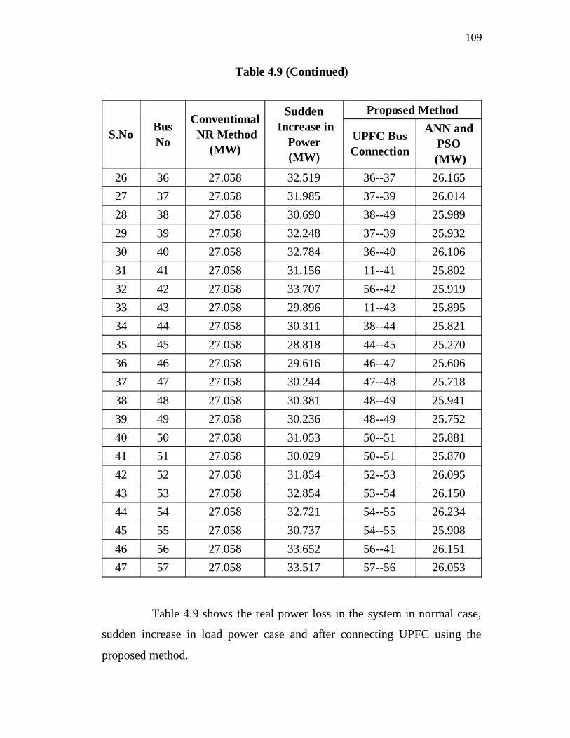
Table 4.9 (Continued)
S.No Bus No
Conventional NR Method
(MW)
Sudden Increase in
Power (MW)
Proposed Method
UPFC Bus Connection
ANN and PSO
(MW) 26 36 27.058 32.519 36--37 26.16527 37 27.058 31.985 37--39 26.01428 38 27.058 30.690 38--49 25.98929 39 27.058 32.248 37--39 25.93230 40 27.058 32.784 36--40 26.10631 41 27.058 31.156 11--41 25.80232 42 27.058 33.707 56--42 25.91933 43 27.058 29.896 11--43 25.89534 44 27.058 30.311 38--44 25.82135 45 27.058 28.818 44--45 25.27036 46 27.058 29.616 46--47 25.60637 47 27.058 30.244 47--48 25.71838 48 27.058 30.381 48--49 25.94139 49 27.058 30.236 48--49 25.75240 50 27.058 31.053 50--51 25.88141 51 27.058 30.029 50--51 25.87042 52 27.058 31.854 52--53 26.09543 53 27.058 32.854 53--54 26.15044 54 27.058 32.721 54--55 26.23445 55 27.058 30.737 54--55 25.90846 56 27.058 33.652 56--41 26.15147 57 27.058 33.517 57--56 26.053
Table 4.9 shows the real power loss in the system in normal case,
sudden increase in load power case and after connecting UPFC using the
proposed method.
110
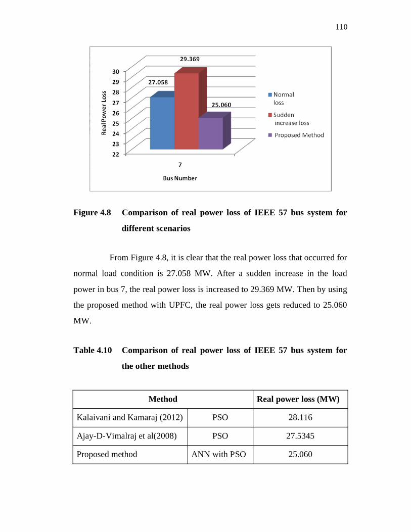
Figure 4.8 Comparison of real power loss of IEEE 57 bus system for
different scenarios
From Figure 4.8, it is clear that the real power loss that occurred for
normal load condition is 27.058 MW. After a sudden increase in the load
power in bus 7, the real power loss is increased to 29.369 MW. Then by using
the proposed method with UPFC, the real power loss gets reduced to 25.060
MW.
Table 4.10 Comparison of real power loss of IEEE 57 bus system for
the other methods
Method Real power loss (MW)
Kalaivani and Kamaraj (2012) PSO 28.116
Ajay-D-Vimalraj et al(2008) PSO 27.5345
Proposed method ANN with PSO 25.060
111
From Table 4.10, it becomes clear that the proposed method obtains
10.87 % of loss reduction compared to GA value reported a in Kalaivani and
Kamaraj (2012) and 8.99 % of loss reduction compared to GA value
mentioned in Ajay-D-Vimalraj et al (2008). This shows the effectiveness of
the proposed approach that minimizes the real power loss compared to the
other methods.
4.6.4 IEEE 118 Bus System
The test system consists of 54 generator buses (bus no. 1, 4, 6, 8,
10, 12, 15, 18, 19, 24, 25, 26, 27, 31, 32, 34, 36, 40, 42, 46, 49, 54, 55, 56, 59,
61, 62, 65, 66, 69, 70, 72, 73, 74, 76, 77, 80, 85, 87, 89, 90, 91, 92, 99, 100,
103, 104, 105, 107, 110, 111, 112, 113, 116) , 64 load buses (bus no. 2, 3, 5,
7, 9, 11, 13, 14, 16, 17, 20, 21, 22, 23, 28, 29, 30, 33, 35, 37, 38, 39, 41, 43,
44, 45, 47, 48, 50, 51, 52, 53, 57, 58, 60, 63, 64, 67, 68, 71, 75, 78, 79, 81, 82,
83, 84, 86, 88, 93, 94, 95, 96, 97, 98, 101,102, 106, 108, 109, 114, 115, 117,
118), 86 transmission lines and bus no. 69 is slack bus. The base MVA
considered is 100 MVA. In bus number 17, the optimal location for
connecting UPF using the proposed method is buses 15 and 17.
A comparison of the voltage profile and real power loss of IEEE
118 bus system for different loading conditions is shown in Figures 4.9 and
4.10 respectively.
112
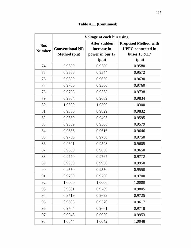
Table 4.11 Voltage profile of IEEE 118 bus system for different conditions
Bus Number
Voltage at each bus using
Conventional NR Method (p.u)
After sudden increase in
power in bus 17 (p.u)
Proposed Method with UPFC connected in
buses 15 &17 (p.u)
1 0.9550 0.9550 0.95502 0.9648 0.9647 0.96493 0.9659 0.9657 0.96584 1.0080 1.0080 1.00805 1.0030 1.0030 1.00306 0.9800 0.9800 0.98107 0.9793 0.9792 0.97948 0.9850 0.9850 0.98509 1.0016 1.0012 1.0016
10 1.0200 1.0200 1.025011 0.9801 0.9799 0.980212 0.9800 0.9800 0.980013 0.9609 0.9603 0.961014 0.9726 0.9725 0.972715 0.9600 0.9600 0.960016 0.9708 0.9704 0.972017 0.9787 0.9781 0.979918 0.9630 0.9630 0.963019 0.9720 0.9720 0.972020 0.9606 0.9601 0.963121 0.9579 0.9571 0.958722 0.9664 0.9657 0.967323 0.9953 0.9950 0.995724 1.0020 1.0020 1.0020
113
Table 4.11 (Continued)
Bus Number
Voltage at each bus using
Conventional NR Method (p.u)
After sudden increase in
power in bus 17 (p.u)
Proposed Method with UPFC connected in
buses 15 &17 (p.u)
25 1.0200 1.0200 1.020026 0.9650 0.9650 0.965027 0.9580 0.9580 0.958028 0.9508 0.9507 0.950929 0.9528 0.9527 0.952830 0.9526 0.9516 0.952931 0.9570 0.9570 0.957032 0.9730 0.9730 0.973033 0.9612 0.9609 0.961434 0.9840 0.9840 0.984035 0.9710 0.9709 0.971136 0.9700 0.9700 0.970037 0.9839 0.9838 0.983938 0.9367 0.9360 0.938939 0.9478 0.9476 0.947840 0.9400 0.9400 0.940041 0.9308 0.9306 0.930942 0.9350 0.9350 0.935043 0.9509 0.9502 0.950944 0.9274 0.9263 0.928545 0.9298 0.9288 0.929946 0.9650 0.9650 0.965047 0.9752 0.9751 0.975348 0.9656 0.9654 0.9658

114
Table 4.11 (Continued)
Bus Number
Voltage at each bus using
Conventional NR Method (p.u)
After sudden increase in
power in bus 17 (p.u)
Proposed Method with UPFC connected in
buses 15 &17 (p.u)
49 0.9750 0.9750 0.975050 0.9543 0.9540 0.954751 0.9239 0.9233 0.923952 0.9246 0.9239 0.924853 0.9290 0.9284 0.930054 0.9250 0.9250 0.925055 0.9220 0.9220 0.922056 0.9240 0.9230 0.926057 0.9324 0.9322 0.933658 0.9310 0.9310 0.935059 0.9550 0.9550 0.955060 0.9966 0.9966 0.996661 1.0050 1.0050 1.005062 0.9880 0.9880 0.988063 0.9492 0.9491 0.949564 0.9691 0.9691 0.969165 0.9750 0.9750 0.975066 1.0200 1.0200 1.020067 0.9979 0.9977 0.998368 0.9892 0.9892 0.989269 1.0350 1.0350 1.035070 0.9740 0.9740 0.974071 0.9785 0.9785 0.978572 0.9900 0.9900 0.990073 0.9810 0.9810 0.9810
115
Table 4.11 (Continued)
Bus Number
Voltage at each bus using
Conventional NR Method (p.u)
After sudden increase in
power in bus 17 (p.u)
Proposed Method with UPFC connected in
buses 15 &17 (p.u)
74 0.9580 0.9580 0.958075 0.9566 0.9544 0.957276 0.9630 0.9630 0.963077 0.9760 0.9560 0.976078 0.9738 0.9558 0.973879 0.9804 0.9669 0.983480 1.0300 1.0300 1.030081 0.9830 0.9829 0.983282 0.9580 0.9495 0.959583 0.9569 0.9508 0.957984 0.9636 0.9616 0.964685 0.9750 0.9750 0.975086 0.9601 0.9598 0.960587 0.9650 0.9650 0.965088 0.9770 0.9767 0.977289 0.9950 0.9950 0.995090 0.9550 0.9550 0.955091 0.9700 0.9700 0.970092 1.0000 1.0000 1.000093 0.9801 0.9789 0.980594 0.9719 0.9699 0.972595 0.9603 0.9570 0.961796 0.9704 0.9661 0.971897 0.9943 0.9920 0.995398 1.0044 1.0042 1.0048
116
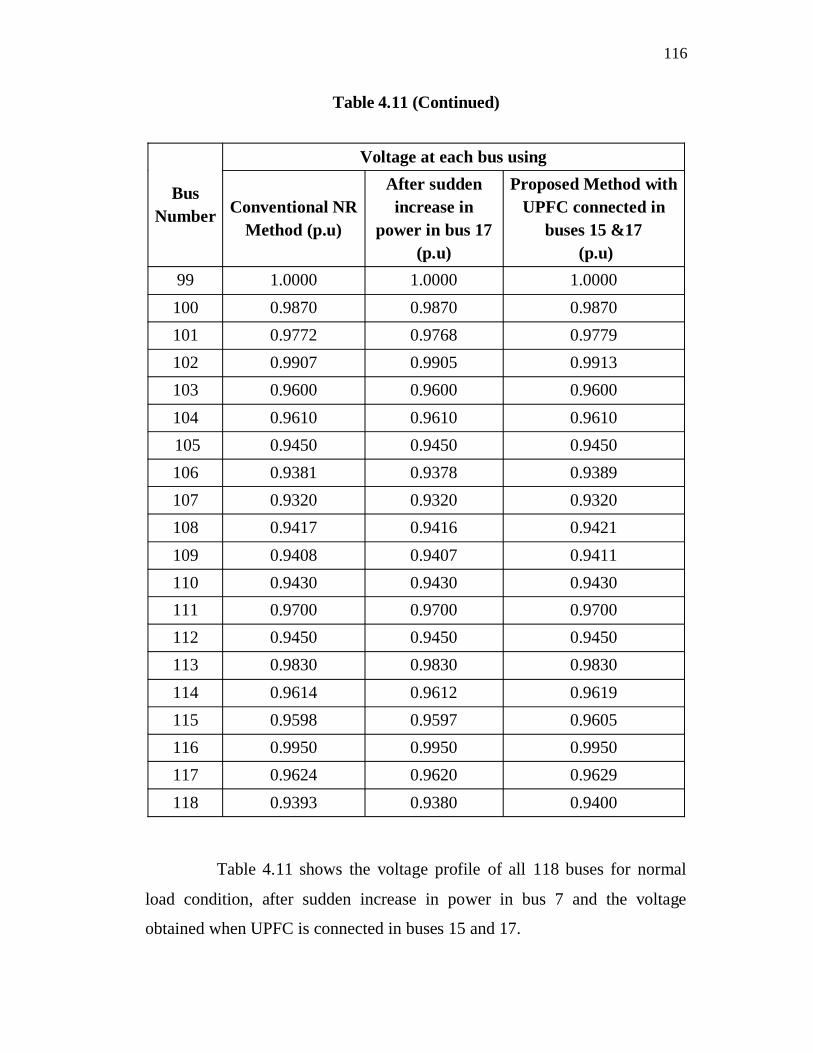
Table 4.11 (Continued)
Bus Number
Voltage at each bus using
Conventional NR Method (p.u)
After sudden increase in
power in bus 17 (p.u)
Proposed Method with UPFC connected in
buses 15 &17 (p.u)
99 1.0000 1.0000 1.0000100 0.9870 0.9870 0.9870101 0.9772 0.9768 0.9779102 0.9907 0.9905 0.9913103 0.9600 0.9600 0.9600104 0.9610 0.9610 0.9610 105 0.9450 0.9450 0.9450106 0.9381 0.9378 0.9389107 0.9320 0.9320 0.9320108 0.9417 0.9416 0.9421109 0.9408 0.9407 0.9411110 0.9430 0.9430 0.9430111 0.9700 0.9700 0.9700112 0.9450 0.9450 0.9450113 0.9830 0.9830 0.9830114 0.9614 0.9612 0.9619115 0.9598 0.9597 0.9605116 0.9950 0.9950 0.9950117 0.9624 0.9620 0.9629118 0.9393 0.9380 0.9400
Table 4.11 shows the voltage profile of all 118 buses for normal
load condition, after sudden increase in power in bus 7 and the voltage
obtained when UPFC is connected in buses 15 and 17.
117
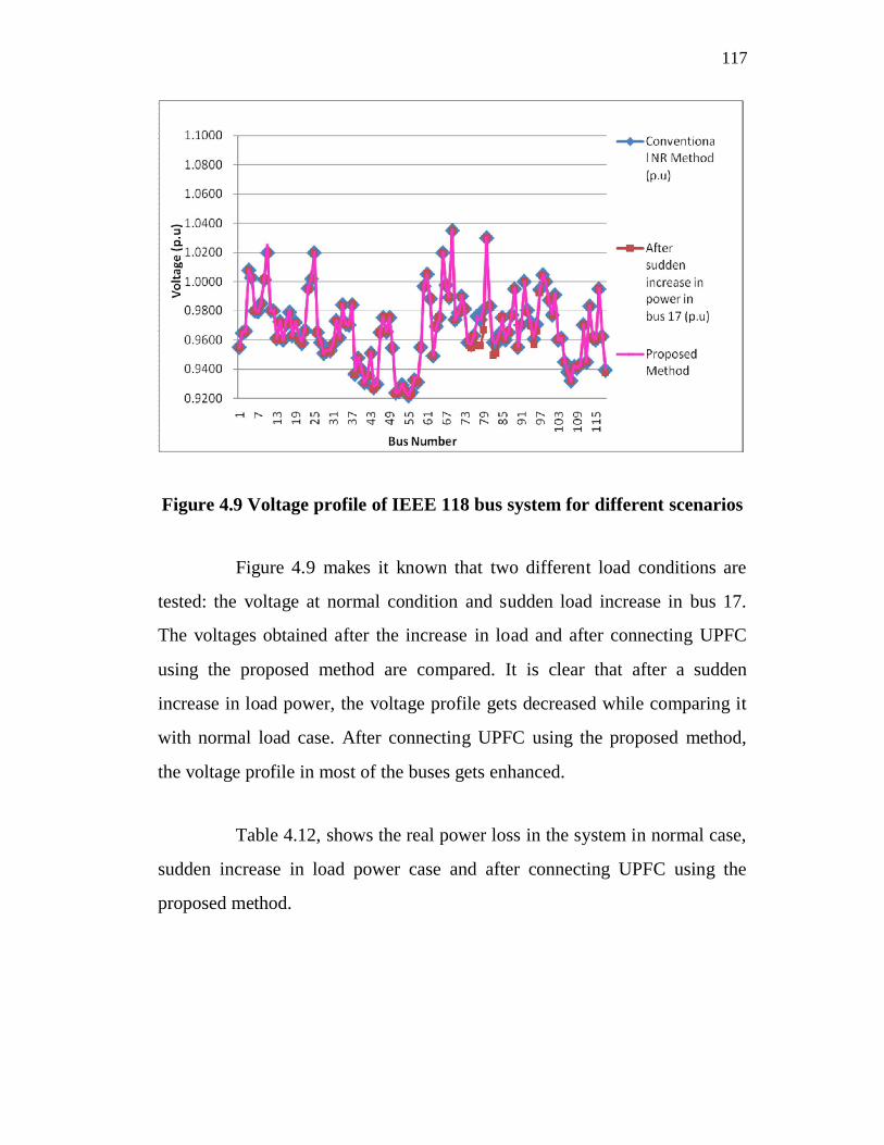
Figure 4.9 Voltage profile of IEEE 118 bus system for different scenarios
Figure 4.9 makes it known that two different load conditions are
tested: the voltage at normal condition and sudden load increase in bus 17.
The voltages obtained after the increase in load and after connecting UPFC
using the proposed method are compared. It is clear that after a sudden
increase in load power, the voltage profile gets decreased while comparing it
with normal load case. After connecting UPFC using the proposed method,
the voltage profile in most of the buses gets enhanced.
Table 4.12, shows the real power loss in the system in normal case,
sudden increase in load power case and after connecting UPFC using the
proposed method.
118
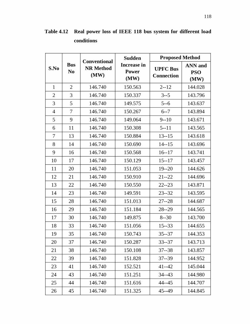
Table 4.12 Real power loss of IEEE 118 bus system for different load
conditions
S.NoBus No
Conventional NR Method
(MW)
Sudden Increase in
Power (MW)
Proposed Method
UPFC Bus Connection
ANN and PSO
(MW) 1 2 146.740 150.563 2--12 144.0282 3 146.740 150.337 3--5 143.7963 5 146.740 149.575 5--6 143.6374 7 146.740 150.267 6--7 143.8945 9 146.740 149.064 9--10 143.6716 11 146.740 150.308 5--11 143.5657 13 146.740 150.884 13--15 143.6188 14 146.740 150.690 14--15 143.6969 16 146.740 150.568 16--17 143.74110 17 146.740 150.129 15--17 143.45711 20 146.740 151.053 19--20 144.62612 21 146.740 150.910 21--22 144.69613 22 146.740 150.550 22--23 143.87114 23 146.740 149.591 23--32 143.59515 28 146.740 151.013 27--28 144.68716 29 146.740 151.184 28--29 144.56517 30 146.740 149.875 8--30 143.70018 33 146.740 151.056 15--33 144.65519 35 146.740 150.743 35--37 144.35320 37 146.740 150.287 33--37 143.71321 38 146.740 150.108 37--38 143.85722 39 146.740 151.828 37--39 144.95223 41 146.740 152.521 41--42 145.04424 43 146.740 151.251 34--43 144.98025 44 146.740 151.616 44--45 144.70726 45 146.740 151.325 45--49 144.845
119
Table 4.12 (Continued)
S.No Bus No
Conventional NR Method
(MW)
Sudden Increase in
Power (MW)
Proposed Method
UPFC Bus Connection
ANN and PSO
(MW) 27 47 146.740 149.812 47--69 143.79828 48 146.740 149.892 48--49 143.64529 50 146.740 150.214 50--57 143.89330 51 146.740 151.113 49--51 144.67731 52 146.740 151.521 52--53 144.72132 53 146.740 151.572 53--54 144.82833 57 146.740 150.974 50--57 144.73334 58 146.740 151.296 56--58 144.82135 60 146.740 149.031 60--62 143.77736 63 146.740 149.215 59--63 143.73237 64 146.740 149.911 64--65 143.75338 67 146.740 150.874 62--67 144.36239 68 146.740 149.823 68--81 143.75240 71 146.740 150.221 71--72 143.76541 75 146.740 150.574 69--75 144.32642 78 146.740 149.728 78--79 143.64243 79 146.740 150.993 79--80 144.61944 81 146.740 149.875 68--81 143.92445 82 146.740 149.119 77--82 143.62246 83 146.740 150.825 83--85 144.41947 84 146.740 149.203 84--85 143.63948 86 146.740 150.945 85--86 144.71449 88 146.740 149.943 85--88 143.69050 93 146.740 149.681 92--93 143.91351 94 146.740 150.416 92--94 144.01452 95 146.740 150.783 94--95 144.27353 96 146.740 149.764 80--96 143.819
120
Table 4.12 (Continued)
S.No Bus No
Conventional NR Method
(MW)
Sudden Increase in
Power (MW)
Proposed Method
UPFC Bus Connection
ANN and PSO
(MW) 54 97 146.740 150.084 80--97 143.72255 98 146.740 149.604 98--100 143.89456 101 146.740 150.116 101--102 143.75257 102 146.740 149.262 92--102 143.83058 106 146.740 149.577 100--106 143.93859 108 146.740 149.893 108--109 143.68560 109 146.740 150.037 109--110 143.89961 114 146.740 150.914 32--114 144.43562 115 146.740 150.921 27--115 144.52963 117 146.740 150.987 12--117 144.82764 118 146.740 151.065 75--118 144.791
.
Figure 4.10 Comparison of real power loss of IEEE 118 bus system for
different scenarios
121
From Figure 4.10, it is clear that the real power loss that occurred
for normal load condition is 146.740 MW. After the sudden increase in the
load power in bus 17, the real power loss is increased to 150.129 MW and
then by using the proposed method with UPFC, the real power loss get
reduced to 143.457 MW.
Table 4.13 Comparison of real power loss of IEEE 118 bus system for other methods
Method Real power loss (MW)
Kalaivani and Kamaraj (2012) PSO 148.00
Proposed method ANN with PSO 143.457
Table 4.13 expresses the fact that the proposed method obtains 3.07
% of loss reduction compared to GA value reported in Kalaivani and Kamaraj
(2012). This shows the effectiveness of the proposed approach which
minimizes the real power loss compared to the other method.
4.7 SUMMARY
This chapter has focused the following: A hybrid technique is used
to identify the location for fixing UPFC in the system and also to compute the
voltage and angle injecting values for enhancing the voltage stability of the
system. The proposed techniques are implemented in MATLAB and tested
using IEEE 14, 30, 57 and 118 bus systems. The performances of the
proposed techniques are analyzed by increasing the load power in the system.
Due to the sudden increase in load power, the voltage profile is decreased and
also the total power loss in the system gets increased. By using the suggested
procedure, the voltage profile gets enhanced along with a reduction in power
loss compared to the other methods.