Chapter 4: CONTINUOUS RANDOMVARIABLES ANDPROBABILITY DISTRIBUTIONS

Part 4:Gamma DistributionWeibull DistributionLognormal DistributionSections 4-9 through 4-11

Another exponential distribution example first...

1

• Example: Magnitude of Earthquakes

The magnitude of earthquakes in a regioncan be modeled as having an exponential dis-tribution where the mean of the distributionis 2.4, as measured on the Richter scale.

Let X represent the magnitude of an earth-quake. Then, X ∼ exponential(λ).

First, determine λ:

E(X) =1

λ= 2.4 ⇒ λ =

1

2.4≈ 0.4167

In this problem, X is not a ‘wait time’ and isnot related to the Poisson process. Here, λ isnot a rate parameter, but is simply a parame-ter that tells you the shape of the distributionof earthquake magnitudes.

2

x

f(x)

0 2 4 6 8 10

Find the probability that an earthquake strik-ing this region will...

a) exceed 3.0 on the Richter scale.

b) fall between 2.0 and 3.0 on the Richterscale.

3

a) exceed 3.0 on the Richter scale.

b) fall between 2.0 and 3.0 on the Richterscale.

4

Gamma DistributionSection 4-9

Another continuous distribution on x > 0 is thegamma distribution.

•Gamma DistributionThe random variableX with probability den-sity function

f (x) =λrxr−1e−λx

Γ (r)for x > 0

is a gamma random variable with parame-ters λ > 0 and r > 0.

•Mean and VarianceFor a gamma random variable with parame-ters λ and r,

µ = E(X) =r

λ

5

andσ2 = V (X) =

r

λ2

• The Gamma function: Γ (r)The value in the denominator of f (x) is aconstant dependent on r. This value is:

Γ (r) =

∫ ∞0

xr−1e−xdx for r > 0

and this is a finite integral.

You can think of Γ (r) as a necessary con-stant in f (x) to make sure the area underf (x) is 1.0

6

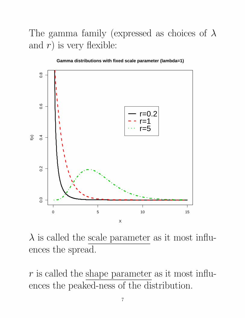
The gamma family (expressed as choices of λand r) is very flexible:

0 5 10 15

0.0

0.2

0.4

0.6

0.8

Gamma distributions with fixed scale parameter (lambda=1)

X

f(x)

r=0.2r=1r=5

λ is called the scale parameter as it most influ-ences the spread.

r is called the shape parameter as it most influ-ences the peaked-ness of the distribution.

7

• Example: Gene expression data

As technology progresses, so does the kind ofdata we can collect. We can now gather in-formation on the amount of protein (or mRNA)outputted by a certain gene in an organism.

Below is a cDNA microarray slide showingthe amount of mRNA (as intensity of fluo-rescence) for each of thousands of genes fora single organism.

8

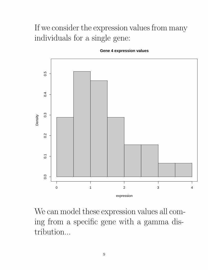
If we consider the expression values from manyindividuals for a single gene:

Gene 4 expression values

expression

Den

sity

0 1 2 3 4

0.0

0.1

0.2

0.3

0.4

0.5

We can model these expression values all com-ing from a specific gene with a gamma dis-tribution...

9

Gene 4 expression values

expression

Den

sity

0 1 2 3 4

0.0

0.1

0.2

0.3

0.4

0.5

The solid curve is the ‘best fitting’ gammadistribution to the observed data.

10

Modeling the observed data with a commondistribution allows us to compute theoreticalprobabilities, and compare different groups(such as healthy patients vs. cancer patients).

——————————————————–

•Gamma distribution modelingexamples:

– Gene expression data

– Climatology models for monthlyprecipitation

– The sum of k independent exponential ran-dom variables

The integration for gamma probabilities wouldcome from tables (like we saw for the normal dis-tribution)... your book does not include these.

11

Instead...

book homework problems are about recognizingthe gamma probability density function, settingup f (x), and recognizing the mean µ and vari-ance σ2 (which can be computed from λ and r),and seeing the connection of the gamma to theexponential and the Poisson process.

• Example: The time between failures of alaser machine is exponentially distributed witha mean of 25,000 hours.

a) What is the expected time until the secondfailure?

12

13

b) What is the probability that the time un-til the third failure exceeds 50,000 hours?

14

15

• Thus, we have another gammadistribution modeling example:

– Time until rth failure in a Poisson Pro-cess with rate parameter λ is distributedgamma(r, λ).

• Some comments on the gamma(r, λ)distribution:

– When r = 1, f (x) is an exponential distri-bution with parameter λ. The exponentialdistribution is a special case of the gammadistribution.

– If r is a positive integer, the distributionis called an Erlang distribution.

16

– Some relationships:

Γ (1) = 0! = 1

Γ (r + 1) = rΓ (r)

Γ (r+1) = r! {Γ (4) = 3·2·1 = 6}

Γ (12) =

√π

– For the gamma(r, λ) distribution, whenλ = 1/2 and r = p/2 where p is a pos-itive integer, then we have a chi-squareddistribution with parameter p, another spe-cial case of the gamma.

17

Weibull DistributionSection 4-10

Another continuous distribution for x > 0.

It can be used to model a situation where thenumber of failures increases with time, decreaseswith time, or remains constant with time. (So,it’s used for more complicated situations than aPoisson process).

•Weibull DistributionThe random variableX with probability den-sity function

f (x) =β

δ

(xδ

)β−1exp

[−(xδ

)β]for x > 0

is a Weibull random variable with scale pa-rameter δ > 0 and shape parameter β > 0.

18

•Mean and VarianceFor a Weibull random variable with param-eters β and δ,

µ = E(X) = δΓ

(1 +

1

β

)and

σ2 = V (X) = δ2Γ

(1 +

2

β

)−δ2

[Γ

(1 +

1

β

)]2

19

Also a flexible family:

20

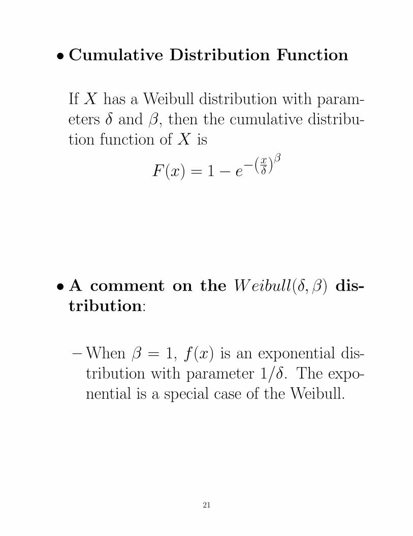
•Cumulative Distribution Function

If X has a Weibull distribution with param-eters δ and β, then the cumulative distribu-tion function of X is

F (x) = 1− e−(xδ)β

•A comment on the Weibull(δ, β) dis-tribution:

– When β = 1, f (x) is an exponential dis-tribution with parameter 1/δ. The expo-nential is a special case of the Weibull.

21

• Example: Manufacture of semiconductor

In an industrial engineering article, the au-thors suggest using a Weibull distribution tomodel the duration of a bake step in the man-ufacture of a semiconductor.

Let T represent the duration in hours of thebake step for a randomly chosen lot.

Suppose T ∼ Weibull(δ = 10, β = 0.3).

a) What is the probability that the bake steptakes longer than four hours?

22

b) What is the probability that the bake steptakes between two and seven hours?

23

Lognormal DistributionSection 4-11

The last continuous distribution we will consideris also for x > 0.

Let W be a normally distributed random vari-able. Suppose we create a new random vari-able X with the transformation X = exp(W ).Then, X is a lognormal random variable. Thename follows from the fact that

ln(X) = W

so we have ln(X) being normally distributed.

W can take on values from −∞ to ∞.

But the domain (or range) of X is the positivereal numbers.

24

• Lognormal Distribution

Let W have a normal distribution with meanθ and variance ω2, then X = exp(W ) is alognormal random variable with probabilitydensity function

f (x) =1

xω√

2πexp

[− (lnx− θ)2

2ω2

]for x > 0.

25

•Mean and VarianceFor a lognormal distribution with parametersθ and ω2,

µ = E(X) = eθ+ω2/2

and

σ2 = V (X) = e2θ+ω2(eω

2− 1)

Note that for the lognormal r.v. X , the meanand variance are µ and σ2 and these arefunctions of θ and ω2, which are the meanand variance of W , a normal random vari-able such that X = exp(W ).

So, θ and ω2 show up in W ∼ N(θ, ω2).

26

• Example: Component lifetimes

Lifetimes of a randomly chosen componentare lognormally distributed with parametersθ = 1 and ω = 0.5 days.

a) Find the mean lifetime of these compo-nents.

b) Find the standard deviation of the life-times.

27

c) Find the probability that a componentlasts longer than 4 days.

28