Chapter 4 Continuous Random Variables and...
29
Chapter 4 Continuous Random Variables and Probability Distributions Part 1: Continuous Random Variables Section 4.1 Continuous Random Variables Section 4.2 Probability Distributions & Probability Density Functions Section 4.3 Cumulative Distribution Functions Section 4.4 Mean and Variance 1 / 29
Transcript of Chapter 4 Continuous Random Variables and...

Chapter 4Continuous Random Variables and ProbabilityDistributions
Part 1: Continuous Random Variables
Section 4.1 Continuous Random VariablesSection 4.2 Probability Distributions & Probability Density FunctionsSection 4.3 Cumulative Distribution FunctionsSection 4.4 Mean and Variance
1 / 29

Continuous Random Variables
Moving on to continuous random variables...
For a continuous random variable X, the range of X includes allvalues in an interval of real numbers. This could be an infiniteinterval such as (−∞,∞).
For example, let X be a random variable such that X can take on anyvalue in the interval [0, 1]. Then, X is a continuous random variable.
2 / 29

Continuous Random Variables
Since there is an infinite number of possible values for X, we describethe probability distribution with a smooth curve.
Example (Continuous random variable)
Suppose X is a random variable such that X ∈ [0, 1], and there is a highprobability that X is near 0.15 and a small probability that X is 0 or 1.Specifically, the distribution of the random variable is shown as:
0.0 0.2 0.4 0.6 0.8 1.0
01
23
4
x
f(x)
This curve is called a probability density function3 / 29

Continuous Random Variables
We can contrast this probability distribution with that of a discreterandom variable which has mass at only ‘distinct’ x-values..
The area under a probability density function is 1. This comparesto the sum of the masses for a discrete random variable being equalto 1.
The probability density function is denoted as f(x), same notation isthe probability mass function, as f(x) describes the distribution of arandom variable.
4 / 29

Continuous Random Variables
Example (Continuous random variable, cont.)
How likely is it that X falls between 0.18 and 0.22?
x
f(x)
0.0 0.2 0.4 0.6 0.8 1.0
We can answer this question by considering the area under the curvebetween 0.18 and 0.22.
This area is approximately 0.1181 for the given f(x) above.5 / 29
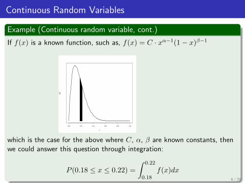
Continuous Random Variables
Example (Continuous random variable, cont.)
If f(x) is a known function, such as, f(x) = C · xα−1(1− x)β−1
x
f(x)
0.0 0.2 0.4 0.6 0.8 1.0
which is the case for the above where C, α, β are known constants, thenwe could answer this question through integration:
P (0.18 ≤ x ≤ 0.22) =
∫ 0.22
0.18f(x)dx
6 / 29

Probability Density Function
Definition (Probability Density Function)
For a continuous random variable X, a probability density function is afunction such that
1 f(x) ≥ 0 (above the horizontal axis)
2∫∞−∞ f(x)dx = 1 (area under curve is equal to 1)
3 P (a ≤ x ≤ b) =∫ ba f(x)dx
= area under f(x) from a to b for any a and b
A probability density function is zero for x values that cannot occur,and it is assumed to be zero wherever it is not specifically defined.
We use f(x) to calculate a probability through integration.
7 / 29

Probability Density Function
In the continuous case, every distinct x-value has zero width (there’sinfinitely many of them), and the probability for a single specificx-value is zero...
P (X = x) = 0.
Instead, we find probabilities for intervals of the random variable, notsingular specific values, like P (0.18 ≤ X ≤ 0.20).
For example, consider weight.
Without the rounding, we see weight as acontinuous variable, and there are an infinite number of possibleweights in (0,∞). On this perception, we could show the distributionof weights using a probability density function.
8 / 29
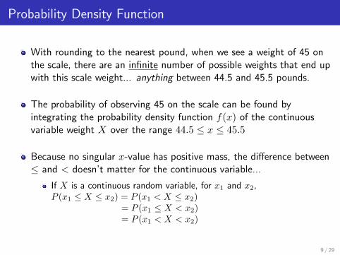
Probability Density Function
With rounding to the nearest pound, when we see a weight of 45 onthe scale, there are an infinite number of possible weights that end upwith this scale weight... anything between 44.5 and 45.5 pounds.
The probability of observing 45 on the scale can be found byintegrating the probability density function f(x) of the continuousvariable weight X over the range 44.5 ≤ x ≤ 45.5
Because no singular x-value has positive mass, the difference between≤ and < doesn’t matter for the continuous variable...
If X is a continuous random variable, for x1 and x2,P (x1 ≤ X ≤ x2) = P (x1 < X ≤ x2)
= P (x1 ≤ X < x2)= P (x1 < X < x2)
9 / 29

Some Probability Density Functions
There are many common probability density functions with knownf(x)...
Normal Density Uniform Density Exponential Density
x
f(x)
0 1 2 3 4 5 60.0
0.2
0.4
0.6
0.8
1.0
x
f(x)
x
f(x)
Gamma Density Log-normal Density Weibull Density
x
f(x)
x
f(x)
x
f(x)
10 / 29

Probability Density Function
But they can also take on unusual shapes too...
Example (Proportion of people returning a survey)
The proportion of people who respond to a certain mail-order solicitationis a continuous random variable X that has density function
f(x) =
{2(x+2)
5 0 < x < 10 otherwise
1 Plot f(x)
2 Show that P (0 < x < 1) = 1
3 Find the probability that more than 1/4 but fewer than 1/2 of the peoplecontacted will respond to this type of solicitation.
11 / 29
Probability Density Function
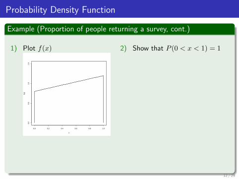
Example (Proportion of people returning a survey, cont.)
1) Plot f(x)
0.0 0.2 0.4 0.6 0.8 1.0
0.0
0.5
1.0
1.5
x
f(x)
2) Show that P (0 < x < 1) = 1
12 / 29

Probability Density Function
Example (Proportion of people returning a survey, cont.)
3) Find the probability that more than 1/4 but fewer than 1/2 of thepeople contacted will respond to this type of solicitation.
13 / 29

Probability Density Function
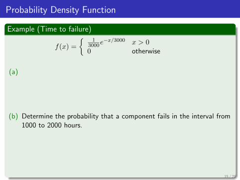
Example (Time to failure)
The probability density function of the time to failure of an electroniccomponent in a copier (in hours) is
f(x) =
{1
3000e−x/3000 x > 0
0 otherwise
(a) What does f(x) look like?
(b) Determine the probability that a component fails in the interval from1000 to 2000 hours.
(c) At what time do we expect 10% of the components to have failed
14 / 29
Probability Density Function
Example (Time to failure)
f(x) =
{1
3000e−x/3000 x > 0
0 otherwise
(a)
(b) Determine the probability that a component fails in the interval from1000 to 2000 hours.
15 / 29
Probability Density Function
Example (Time to failure, cont.)
f(x) =
{1
3000e−x/3000 x > 0
0 otherwise
(c) At what time do we expect 10% of the components to have failed
16 / 29

Probability Density Function - ESPN examples
Example (Fantasy football point distributions)
Alvin Karama (RB) Jake Elliott (K)
NOTE: Don’t look at the y-axis stated ‘probability %’, not relevant as probabilities are areas under the curve.
17 / 29

Cumulative Distribution Functions
As we did with discrete random variables, we often want to computethe cumulative probabilities, or P (X ≤ x).
Definition (Cumulative Distribution Function)
The cumulative distribution function (CDF) of a continuous randomvariable X is
F (x) = P (X ≤ x) =∫ x
−∞f(u)du
for −∞ < x <∞.
To find F (x), find the anti-derivative of f(x)
And vice versa...If you’re given F (x), you can find f(x) through
differentiation as f(x) =dF (x)dx .
18 / 29
Cumulative Distribution Functions
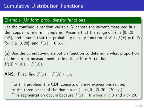
Example (Uniform prob. density function)
Let the continuous random variable X denote the current measured in athin copper wire in milliamperes. Assume that the range of X is [0, 20mA], and assume that the probability density function of X is f(x) = 0.05for x ∈ [0, 20], and f(x) = 0 o.w.
(a) Use the cumulative distribution function to determine what proportionof the current measurements is less than 10 mA, i.e. findP (X ≤ 10) = F (10).
ANS: First, find F (x) = P (X ≤ x).
For this problem, the CDF consists of three expressions relatedto the three pieces of the domain as (−∞, 0), [0, 20], (20,∞).This segmentation occurs because f(x) = 0 when x < 0 and x > 20.
19 / 29

Cumulative Distribution Functions
Example (Uniform prob. density function, cont.)
We know F (x)=0 for x<0 (no probability accumulated left of x = 0) andF (x)=1 for x ≥ 20 (all probability accumulated by x = 20).
Now we just need to define F (x) in [0, 20] . . .
[0, 20] : F (x) = P (X ≤ x) =∫ x0 f(u)du
=∫ x0 0.05du
= 0.05u|x0 = 0.05xThus,
F (x) =
0 x < 00.05x 0 ≤ x ≤ 201 x > 20
20 / 29
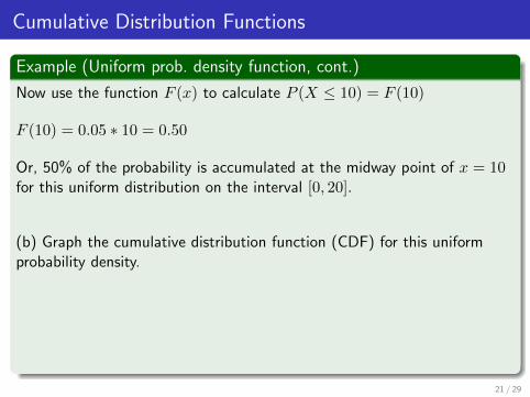
Cumulative Distribution Functions
Example (Uniform prob. density function, cont.)
Now use the function F (x) to calculate P (X ≤ 10) = F (10)
F (10) = 0.05 ∗ 10 = 0.50
Or, 50% of the probability is accumulated at the midway point of x = 10for this uniform distribution on the interval [0, 20].
(b) Graph the cumulative distribution function (CDF) for this uniformprobability density.
21 / 29

Cumulative Distribution Functions
Example (Uniform prob. density function, cont.)
A cumulative distribution function (CDF) describes how probability isaccumulated as x goes from left to right or from −∞ to +∞.
In the uniform distribution case above, we accumulate probability at aconstant rate (thus, the straight line).
22 / 29

Cumulative Distribution Functions
Example (Recall the Time to Failure example...)
The probability density function of the time to failure of an electroniccomponent in a copier (in hours) is
f(x) =
{1
3000e−x/3000 x > 0
0 otherwise
PDF or f(x)
x
f(x)
0 2000 4000 6000 8000 10000
Meant to represent50% of the area under the curve
Determine the cumulative distribution function (CDF) from f(x) and useit to calculate when 50% of the components have failed.
23 / 29
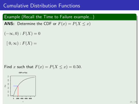
Cumulative Distribution Functions
Example (Recall the Time to Failure example...)
ANS: Determine the CDF or F (x) = P (X ≤ x)
(−∞, 0) : F (X) = 0
[ 0,∞) : F (X) =
Find x such that F (x) = P (X ≤ x) = 0.50.
0 2000 4000 6000 8000
0.0
0.2
0.4
0.6
0.8
1.0
CDF or F(x)
x
F(x)
0 2000 4000 6000 8000
24 / 29

Continuous Random Variables
The mean and variance of continuous random variables can becomputed similar to those for discrete random variables, but forcontinuous random variables, we will be integrating over the domainof X rather than summing over the possible values of X.
Definition (Mean and Variance of Continuous Random Variable)
Suppose X is a continuous random variable with probability densityfunction f(x). The mean or expected value of X, denoted as µ or E(X),is
µ = E(X) =
∫ ∞−∞
xf(x)dx
25 / 29
Continuous Random Variables
Definition (Mean and Variance of a Continuous Random Variable)
The variance of X, denoted as V (X) or σ2, is
σ2 = V (X) =E(X − µ)2
=E(X2)− (EX)2
=
∫ ∞−∞
(x− µ)2f(x)dx
=
∫ ∞−∞
x2f(x)dx− µ2
The standard deviation of X is σ =√σ2
26 / 29
Continuous Random Variables
Example (Mean and Variance of a Continuous Random Variable)
For the uniform probability density function described earlier, f(x) = 0.05for 0 ≤ x ≤ 20, compute E(X) and V (X).
ANS:
27 / 29

Continuous Random Variables
Definition (Expected Value of a Function)
If X is a continuous variable with probability density function f(x),
E[h(x)] =
∫ ∞−∞
h(x)f(x)dx
Example (Weight of delivered packages (p. 115 problem 4-36))
The probability density function of the weight of packages delivered by apost office is
f(x) = 70/(69x2) for 1 < x < 70 pounds.
If the cost is $2.50 per pound, what is the mean shipping cost of apackage?
28 / 29

Continuous Random Variables
Example (Weight of delivered packages (p. 115 problem 4-36), cont.)
f(x) = 70/(69x2) for 1 < x < 70 pounds.
If the cost is $2.50 per pound, what is the mean shipping cost of apackage?
ANS:
29 / 29