Chapter 4: Computation tree logic · INFOF412 Formal veri cation of computer systems Chapter 4:...
74
INFOF412 · Formal verification of computer systems Chapter 4: Computation tree logic Mickael Randour Formal Methods and Verification group Computer Science Department, ULB March 2017
-
Upload
truongdung -
Category
Documents
-
view
215 -
download
0
Transcript of Chapter 4: Computation tree logic · INFOF412 Formal veri cation of computer systems Chapter 4:...
INFOF412 · Formal verification of computer systems
Chapter 4: Computation tree logic
Mickael RandourFormal Methods and Verification group
Computer Science Department, ULB
March 2017
CTL CTL model checking CTL vs. LTL CTL∗
1 CTL: a specification language for BT properties
2 CTL model checking
3 CTL vs. LTL
4 CTL∗
Chapter 4: Computation tree logic Mickael Randour 1 / 71

CTL CTL model checking CTL vs. LTL CTL∗
1 CTL: a specification language for BT properties
2 CTL model checking
3 CTL vs. LTL
4 CTL∗
Chapter 4: Computation tree logic Mickael Randour 2 / 71
CTL CTL model checking CTL vs. LTL CTL∗
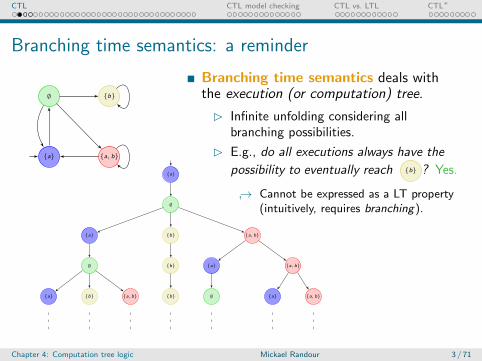
Branching time semantics: a reminder
{a}
∅
{a, b}
{b}
Branching time semantics deals withthe execution (or computation) tree.
� Infinite unfolding considering allbranching possibilities.
� E.g., do all executions always have the
possibility to eventually reach {b} ? Yes.
↪→ Cannot be expressed as a LT property(intuitively, requires branching).
{a}
∅
{a} {b}
{b}
{b}
{a, b}
∅ {a} {a, b}
{a} {b} {a, b} ∅ {a} {a, b}
Chapter 4: Computation tree logic Mickael Randour 3 / 71

CTL CTL model checking CTL vs. LTL CTL∗
IntuitionIn LTL, s |= φ means that all paths starting is s satisfy φ.
� Implicit universal quantification.� Could be made explicit by writing s |= ∀φ.
What if we want to talk about some paths?� E.g., does there exist a path satisfying φ starting in s?� Could be expressed using the duality between universal and
existential quantification: s |= ∃φ iff s 6|= ∀¬φ.
What if the property is more complex? E.g., do all executionsalways have the possibility to eventually reach {b} ?
� s |= ∀�♦b does not work as it requires all paths to always
return in {b} , not just to have the possibility to do so.
� Not expressible in LTL. We need nesting of pathquantifiers (∀,∃).
↪→ s |= ∀�∃♦b is a CTL formula: “for all paths, it is always thecase (i.e., at every step along the branch) that there exists apath (which can be branching) that eventually reaches b.”
Chapter 4: Computation tree logic Mickael Randour 4 / 71
CTL CTL model checking CTL vs. LTL CTL∗
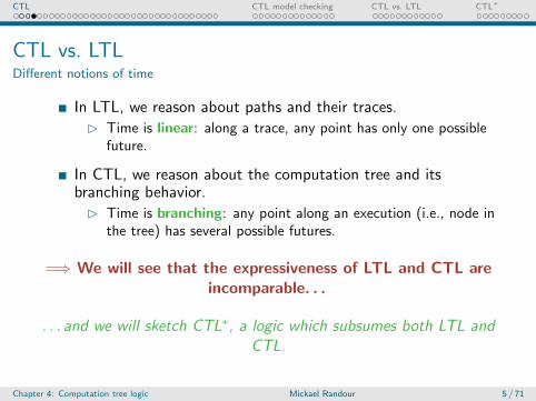
CTL vs. LTLDifferent notions of time
In LTL, we reason about paths and their traces.
� Time is linear: along a trace, any point has only one possiblefuture.
In CTL, we reason about the computation tree and itsbranching behavior.
� Time is branching: any point along an execution (i.e., node inthe tree) has several possible futures.
=⇒ We will see that the expressiveness of LTL and CTL areincomparable. . .
. . . and we will sketch CTL∗, a logic which subsumes both LTL andCTL.
Chapter 4: Computation tree logic Mickael Randour 5 / 71
CTL CTL model checking CTL vs. LTL CTL∗
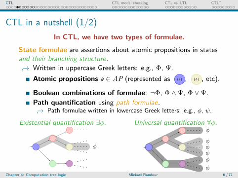
CTL in a nutshell (1/2)
In CTL, we have two types of formulae.
State formulae are assertions about atomic propositions in statesand their branching structure.
↪→ Written in uppercase Greek letters: e.g., Φ, Ψ.
Atomic propositions a ∈ AP (represented as {a} , {b} , etc).
Boolean combinations of formulae: ¬Φ, Φ ∧Ψ, Φ ∨Ψ.
Path quantification using path formulae.↪→ Path formulae written in lowercase Greek letters: e.g., φ, ψ.
Existential quantification ∃φ.
φ
Universal quantification ∀φ.
φφ
φ
φφ
φ
Chapter 4: Computation tree logic Mickael Randour 6 / 71
CTL CTL model checking CTL vs. LTL CTL∗
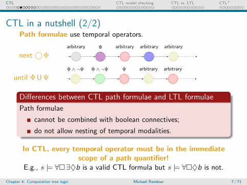
CTL in a nutshell (2/2)Path formulae use temporal operators.
next ©ΦΦarbitrary arbitrary arbitrary arbitrary
until ΦUΨΦ ∧ ¬ΨΦ ∧ ¬Ψ Ψ arbitrary arbitrary
Differences between CTL path formulae and LTL formulae
Path formulae
cannot be combined with boolean connectives;
do not allow nesting of temporal modalities.
In CTL, every temporal operator must be in the immediatescope of a path quantifier!
E.g., s |= ∀�∃♦b is a valid CTL formula but s |= ∀�♦b is not.
Chapter 4: Computation tree logic Mickael Randour 7 / 71
CTL CTL model checking CTL vs. LTL CTL∗
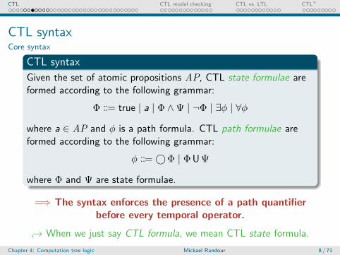
CTL syntaxCore syntax
CTL syntax
Given the set of atomic propositions AP, CTL state formulae areformed according to the following grammar:
Φ ::= true | a | Φ ∧Ψ | ¬Φ | ∃φ | ∀φ
where a ∈ AP and φ is a path formula. CTL path formulae areformed according to the following grammar:
φ ::=©Φ | ΦUΨ
where Φ and Ψ are state formulae.
=⇒ The syntax enforces the presence of a path quantifierbefore every temporal operator.
↪→ When we just say CTL formula, we mean CTL state formula.
Chapter 4: Computation tree logic Mickael Randour 8 / 71
CTL CTL model checking CTL vs. LTL CTL∗
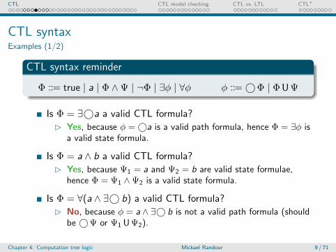
CTL syntaxExamples (1/2)
CTL syntax reminder
Φ ::= true | a | Φ ∧Ψ | ¬Φ | ∃φ | ∀φ φ ::=©Φ | ΦUΨ
Is Φ = ∃©a a valid CTL formula?
� Yes, because φ =©a is a valid path formula, hence Φ = ∃φ isa valid state formula.
Is Φ = a ∧ b a valid CTL formula?
� Yes, because Ψ1 = a and Ψ2 = b are valid state formulae,hence Φ = Ψ1 ∧Ψ2 is a valid state formula.
Is Φ = ∀(a ∧ ∃© b) a valid CTL formula?
� No, because φ = a ∧ ∃© b is not a valid path formula (shouldbe ©Ψ or Ψ1 UΨ2).
Chapter 4: Computation tree logic Mickael Randour 9 / 71
CTL CTL model checking CTL vs. LTL CTL∗
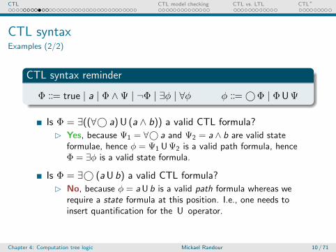
CTL syntaxExamples (2/2)
CTL syntax reminder
Φ ::= true | a | Φ ∧Ψ | ¬Φ | ∃φ | ∀φ φ ::=©Φ | ΦUΨ
Is Φ = ∃((∀© a) U (a ∧ b)) a valid CTL formula?
� Yes, because Ψ1 = ∀© a and Ψ2 = a ∧ b are valid stateformulae, hence φ = Ψ1 UΨ2 is a valid path formula, henceΦ = ∃φ is a valid state formula.
Is Φ = ∃© (aU b) a valid CTL formula?
� No, because φ = aU b is a valid path formula whereas werequire a state formula at this position. I.e., one needs toinsert quantification for the U operator.
Chapter 4: Computation tree logic Mickael Randour 10 / 71
CTL CTL model checking CTL vs. LTL CTL∗
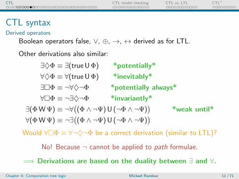
CTL syntaxDerived operators
Boolean operators false, ∨, ⊕, →, ↔ derived as for LTL.
Other derivations also similar:
∃♦Φ ≡ ∃(true UΦ) *potentially*
∀♦Φ ≡ ∀(true UΦ) *inevitably*
∃�Φ ≡ ¬∀♦¬Φ *potentially always*
∀�Φ ≡ ¬∃♦¬Φ *invariantly*
∃(ΦWΨ) ≡ ¬∀((Φ ∧ ¬Ψ) U (¬Φ ∧ ¬Ψ)
)*weak until*
∀(ΦWΨ) ≡ ¬∃((Φ ∧ ¬Ψ) U (¬Φ ∧ ¬Ψ)
)Would ∀�Φ ≡ ∀¬♦¬Φ be a correct derivation (similar to LTL)?
No! Because ¬ cannot be applied to path formulae.
=⇒ Derivations are based on the duality between ∃ and ∀.
Chapter 4: Computation tree logic Mickael Randour 11 / 71

CTL CTL model checking CTL vs. LTL CTL∗
CTL syntaxPrecedence order
Same rules as for LTL, with quantifiers ∃, ∀ directly linked to thefollowing path formula.
Chapter 4: Computation tree logic Mickael Randour 12 / 71
CTL CTL model checking CTL vs. LTL CTL∗
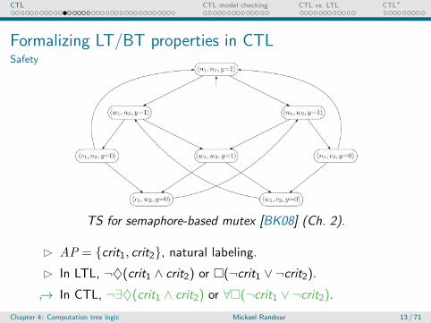
Formalizing LT/BT properties in CTLSafety
TS for semaphore-based mutex [BK08] (Ch. 2).
� AP = {crit1, crit2}, natural labeling.
� In LTL, ¬♦(crit1 ∧ crit2) or �(¬crit1 ∨ ¬crit2).
↪→ In CTL, ¬∃♦(crit1 ∧ crit2) or ∀�(¬crit1 ∨ ¬crit2).
Chapter 4: Computation tree logic Mickael Randour 13 / 71
CTL CTL model checking CTL vs. LTL CTL∗
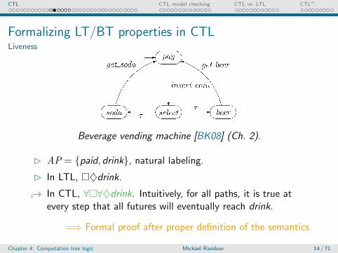
Formalizing LT/BT properties in CTLLiveness
Beverage vending machine [BK08] (Ch. 2).
� AP = {paid, drink}, natural labeling.
� In LTL, �♦drink.
↪→ In CTL, ∀�∀♦drink. Intuitively, for all paths, it is true atevery step that all futures will eventually reach drink.
=⇒ Formal proof after proper definition of the semantics.
Chapter 4: Computation tree logic Mickael Randour 14 / 71
CTL CTL model checking CTL vs. LTL CTL∗
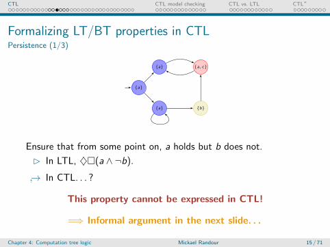
Formalizing LT/BT properties in CTLPersistence (1/3)
{a}
{a}
{a}
{a, c}
{b}
Ensure that from some point on, a holds but b does not.
� In LTL, ♦�(a ∧ ¬b).
↪→ In CTL. . . ?
This property cannot be expressed in CTL!
=⇒ Informal argument in the next slide. . .
Chapter 4: Computation tree logic Mickael Randour 15 / 71

CTL CTL model checking CTL vs. LTL CTL∗
Formalizing LT/BT properties in CTLPersistence (2/3)
Take a simpler TS T :
s1 s2 s3
{a} {b} {a}
It clearly satisfies LTL formulaφ = ♦�a.
As all paths, the highlighted onemust satisfy ♦∀�a for Φ to hold.
But there is no state alongthis path where ∀�a holds aswe can always branch to b!=⇒ T 6|= Φ.
Best guess for equivalent CTLformula: Φ = ∀♦∀�a (we wantthis to be true on all paths).
But what is the executiontree?
Chapter 4: Computation tree logic Mickael Randour 16 / 71

CTL CTL model checking CTL vs. LTL CTL∗
Formalizing LT/BT properties in CTLPersistence (3/3)
Intuition.
In LTL, time is linear .� Either we have a path that do branch to b, thus �a is true
after b. Or we never branch and �a is true from the initialstate.
In CTL, time is branching .� We have to use the ∀ quantifier (as we want to characterize all
paths).� But then ♦∀�a asks to reach a state where all possible
futures satisfy �a.� Not possible because of the possibility of branching.
Hence, even if all branches satisfy ♦�a, the CTL formularequires the additional (and not verified) existence of nodesin the tree whose subtrees only contain paths satisfying �a.
Chapter 4: Computation tree logic Mickael Randour 17 / 71

CTL CTL model checking CTL vs. LTL CTL∗
Formalizing LT/BT properties in CTLTypical BT property
{a}
{a}
{a}
{a, c}
{b}
Along all paths, it is always possible to reach {a, c} .
� Not expressible in LTL: in linear time, either you reach or youdo not. Reasoning about possible futures requires branchingtime.
↪→ In CTL, ∀�∃♦(a ∧ c).
Chapter 4: Computation tree logic Mickael Randour 18 / 71
CTL CTL model checking CTL vs. LTL CTL∗
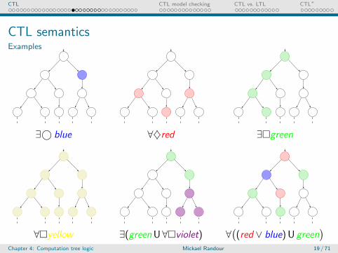
CTL semanticsExamples
∃© blue ∀♦red ∃�green
∀�yellow ∃(green U∀�violet) ∀((red ∨ blue) U green
)Chapter 4: Computation tree logic Mickael Randour 19 / 71
CTL CTL model checking CTL vs. LTL CTL∗
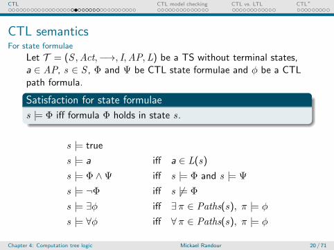
CTL semanticsFor state formulae
Let T = (S ,Act,−→, I,AP,L) be a TS without terminal states,a ∈ AP, s ∈ S , Φ and Ψ be CTL state formulae and φ be a CTLpath formula.
Satisfaction for state formulae
s |= Φ iff formula Φ holds in state s.
s |= true
s |= a iff a ∈ L(s)
s |= Φ ∧Ψ iff s |= Φ and s |= Ψ
s |= ¬Φ iff s 6|= Φ
s |= ∃φ iff ∃π ∈ Paths(s), π |= φ
s |= ∀φ iff ∀π ∈ Paths(s), π |= φ
Chapter 4: Computation tree logic Mickael Randour 20 / 71
CTL CTL model checking CTL vs. LTL CTL∗
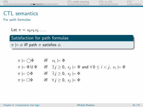
CTL semanticsFor path formulae
Let π = s0s1s2 . . . .
Satisfaction for path formulae
π |= φ iff path π satisfies φ.
π |=©Φ iff s1 |= Φ
π |= ΦUΨ iff ∃ j ≥ 0, s j |= Ψ and ∀ 0 ≤ i < j , s i |= Φ
π |= ♦Φ iff ∃ j ≥ 0, s j |= Φ
π |= �Φ iff ∀ j ≥ 0, s j |= Φ
Chapter 4: Computation tree logic Mickael Randour 21 / 71
CTL CTL model checking CTL vs. LTL CTL∗
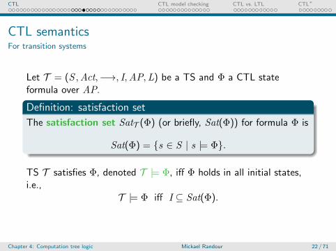
CTL semanticsFor transition systems
Let T = (S ,Act,−→, I,AP,L) be a TS and Φ a CTL stateformula over AP.
Definition: satisfaction set
The satisfaction set SatT (Φ) (or briefly, Sat(Φ)) for formula Φ is
Sat(Φ) = {s ∈ S | s |= Φ}.
TS T satisfies Φ, denoted T |= Φ, iff Φ holds in all initial states,i.e.,
T |= Φ iff I ⊆ Sat(Φ).
Chapter 4: Computation tree logic Mickael Randour 22 / 71
CTL CTL model checking CTL vs. LTL CTL∗
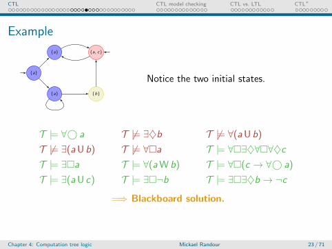
Example
{a}
{a}
{a}
{a, c}
{b}
Notice the two initial states.
T |= ∀© a T 6|= ∃♦b T 6|= ∀(aU b)
T 6|= ∃(aU b) T 6|= ∀�a T |= ∀�∃♦∀�∀♦cT |= ∃�a T |= ∀(aW b) T |= ∀�(c → ∀© a)
T |= ∃(aU c) T |= ∃�¬b T |= ∃�∃♦b → ¬c
=⇒ Blackboard solution.
Chapter 4: Computation tree logic Mickael Randour 23 / 71
CTL CTL model checking CTL vs. LTL CTL∗
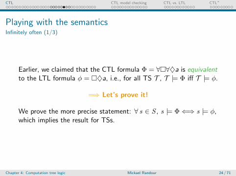
Playing with the semanticsInfinitely often (1/3)
Earlier, we claimed that the CTL formula Φ = ∀�∀♦a is equivalentto the LTL formula φ = �♦a, i.e., for all TS T , T |= Φ iff T |= φ.
=⇒ Let’s prove it!
We prove the more precise statement: ∀ s ∈ S , s |= Φ⇐⇒ s |= φ,which implies the result for TSs.
Chapter 4: Computation tree logic Mickael Randour 24 / 71

CTL CTL model checking CTL vs. LTL CTL∗
Playing with the semanticsInfinitely often (2/3)
s |= Φ =⇒ s |= φ.
1 Let s |= Φ. We must prove that ∀π = s0s1s2 . . . ∈ Paths(s),π |= φ, i.e., for all j ≥ 0, there exists i ≥ j such that s i |= a.
2 Since s |= ∀�∀♦a and π ∈ Paths(s), we have π |= �∀♦a.
3 Hence, s j |= ∀♦a.
4 Since π[j ..] = s js j+1 . . . ∈ Paths(s j), we have thatπ[j ..] |= ♦a.
5 Hence, there exists i ≥ j such that s i |= a.
6 This holds for all j so we are done.
Chapter 4: Computation tree logic Mickael Randour 25 / 71

CTL CTL model checking CTL vs. LTL CTL∗
Playing with the semanticsInfinitely often (3/3)
s |= Φ ⇐= s |= φ.
1 Let s |= φ. We must prove that s |= ∀�∀♦a, i.e, that∀π = s0s1s2 . . . ∈ Paths(s), π |= �∀♦a.
2 I.e., that for all j ≥ 0, s j |= ∀♦a.
3 Let j ≥ 0 and fix any path π′ = s js′j+1s
′j+2 . . . ∈ Paths(s j).
We must show that π′ |= ♦a.
4 But, then π′′ = s0s1 . . . s js′j+1s
′j+2 . . . ∈ Paths(s). Hence,
π′′ |= �♦a by hypothesis.
5 Hence, there exists i > j such that s ′i |= a.
6 Therefore, π′ |= ♦a.
7 This holds for any path π′ ∈ Paths(s j) so s j |= ∀♦a.
8 Since it holds for all j , π |= �∀♦a.
9 Finally, it holds for all π ∈ Paths(s), thus s |= Φ.
Chapter 4: Computation tree logic Mickael Randour 26 / 71

CTL CTL model checking CTL vs. LTL CTL∗
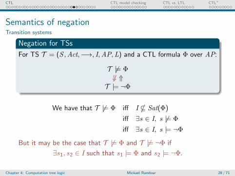
Semantics of negationStates
Negation for states
For s ∈ S and a CTL formula Φ over AP,
s 6|= Φ ⇐⇒ s |= ¬Φ.
Intuitively, due to the duality between ∀ and ∃ and the semanticsof negation for path formulae (see LTL, either a path satisfies φ orit satisfies ¬φ).
Chapter 4: Computation tree logic Mickael Randour 27 / 71
CTL CTL model checking CTL vs. LTL CTL∗
Semantics of negationTransition systems
Negation for TSs
For TS T = (S ,Act,−→, I,AP,L) and a CTL formula Φ over AP:
T 6|= Φ6⇓ ⇑
T |= ¬Φ
We have that T 6|= Φ iff I * Sat(Φ)
iff ∃s ∈ I, s 6|= Φ
iff ∃s ∈ I, s |= ¬Φ
But it may be the case that T 6|= Φ and T 6|= ¬Φ if
∃s1, s2 ∈ I such that s1 |= Φ and s2 |= ¬Φ.
Chapter 4: Computation tree logic Mickael Randour 28 / 71

CTL CTL model checking CTL vs. LTL CTL∗
Semantics of negationExample
s1 s2
{a} ∅
Consider CTL formula Φ = ∃�a. Do we have that T |= Φ?
Beware of erroneous intuition!T |= ∃φ 6⇐⇒ ∃σ ∈ Traces(T ), σ |= φ.
Indeed, Φ must hold in all initial states.
↪→ Here it does not in s2 =⇒ T 6|= Φ.
Do we have that T |= ¬Φ = ∀♦¬a?
↪→ No. Because of path (s1)ω, s1 6|= ¬Φ =⇒ T 6|= ¬Φ.
Surprising equivalence.T 6|= ¬∃φ ⇐⇒ ∃σ ∈ Traces(T ), σ |= φ.
Chapter 4: Computation tree logic Mickael Randour 29 / 71
CTL CTL model checking CTL vs. LTL CTL∗
Equivalence of CTL formulaeDefinition
Equivalence of CTL formulae
CTL (state) formulae Φ and Ψ over AP are equivalent, denotedΦ ≡ Ψ, if and only if, for all TS T over AP,
Sat(Φ) = Sat(Ψ).
In particular, Φ ≡ Ψ ⇐⇒ (∀T , T |= Φ ⇐⇒ T |= Ψ).
=⇒ Let us review some computational rules.
Chapter 4: Computation tree logic Mickael Randour 30 / 71
CTL CTL model checking CTL vs. LTL CTL∗
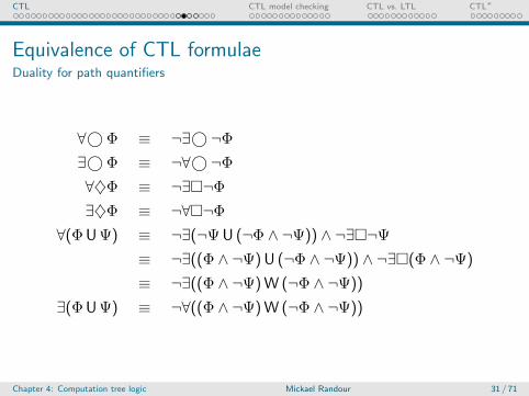
Equivalence of CTL formulaeDuality for path quantifiers
∀© Φ ≡ ¬∃©¬Φ∃© Φ ≡ ¬∀©¬Φ∀♦Φ ≡ ¬∃�¬Φ∃♦Φ ≡ ¬∀�¬Φ
∀(ΦUΨ) ≡ ¬∃(¬ΨU (¬Φ ∧ ¬Ψ)) ∧ ¬∃�¬Ψ≡ ¬∃((Φ ∧ ¬Ψ) U (¬Φ ∧ ¬Ψ)) ∧ ¬∃�(Φ ∧ ¬Ψ)
≡ ¬∃((Φ ∧ ¬Ψ) W (¬Φ ∧ ¬Ψ))
∃(ΦUΨ) ≡ ¬∀((Φ ∧ ¬Ψ) W (¬Φ ∧ ¬Ψ))
Chapter 4: Computation tree logic Mickael Randour 31 / 71
CTL CTL model checking CTL vs. LTL CTL∗
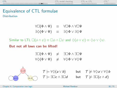
Equivalence of CTL formulaeDistribution
∀�(Φ ∧Ψ) ≡ ∀�Φ ∧ ∀�Ψ
∃♦(Φ ∨Ψ) ≡ ∃♦Φ ∨ ∃♦Ψ
Similar to LTL �(φ ∧ ψ) ≡ �φ ∧�ψ and ♦(φ ∨ ψ) ≡ ♦φ ∨ ♦ψ.
But not all laws can be lifted!
∃�(Φ ∧Ψ) 6≡ ∃�Φ ∧ ∃�Ψ
∀♦(Φ ∨Ψ) 6≡ ∀♦Φ ∨ ∀♦Ψ
{c, d}
{a, c} {b, d}
T |= ∀♦(a ∨ b) but T 6|= ∀♦a ∨ ∀♦bT |= ∃�c ∧ ∃�d but T 6|= ∃�(c ∧ d)
Chapter 4: Computation tree logic Mickael Randour 32 / 71

CTL CTL model checking CTL vs. LTL CTL∗
Equivalence of CTL formulaeExpansion laws
In LTL, we had:
φUψ ≡ ψ ∨ (φ ∧© (φUψ))
♦φ ≡ φ ∨©♦φ�φ ≡ φ ∧©�φ
In CTL, we have:
∀(ΦUΨ) ≡ Ψ ∨ (Φ ∧ ∀© ∀(ΦUΨ))
∀♦Φ ≡ Φ ∨ ∀© ∀♦Φ∀�Φ ≡ Φ ∧ ∀© ∀�Φ
∃(ΦUΨ) ≡ Ψ ∨ (Φ ∧ ∃© ∃(ΦUΨ))
∃♦Φ ≡ Φ ∨ ∃© ∃♦Φ∃�Φ ≡ Φ ∧ ∃© ∃�Φ
Chapter 4: Computation tree logic Mickael Randour 33 / 71

CTL CTL model checking CTL vs. LTL CTL∗
Existential normal form (ENF)ENF for CTL
Goal
Retain the full expressiveness of CTL but permit only existentialquantifiers (thanks to negation and duality).
ENF for CTL
Given atomic propositions AP, CTL formulae in existential normalform are given by:
Φ ::= true | a | Φ ∧Ψ | ¬Φ | ∃© Φ | ∃(ΦUΨ) | ∃�Φ
where a ∈ AP.
Every CTL formula can be rewritten in ENF. . . but thetranslation can cause an exponential blowup (because of therewrite rule for ∀U ).
Chapter 4: Computation tree logic Mickael Randour 34 / 71
CTL CTL model checking CTL vs. LTL CTL∗
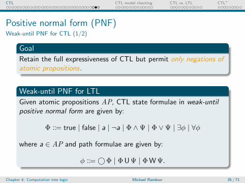
Positive normal form (PNF)Weak-until PNF for CTL (1/2)
Goal
Retain the full expressiveness of CTL but permit only negations ofatomic propositions.
Weak-until PNF for LTL
Given atomic propositions AP, CTL state formulae in weak-untilpositive normal form are given by:
Φ ::= true | false | a | ¬a | Φ ∧Ψ | Φ ∨Ψ | ∃φ | ∀φ
where a ∈ AP and path formulae are given by:
φ ::=©Φ | ΦUΨ | ΦWΨ.
Chapter 4: Computation tree logic Mickael Randour 35 / 71
CTL CTL model checking CTL vs. LTL CTL∗
Positive normal form (PNF)Weak-until PNF for CTL (2/2)
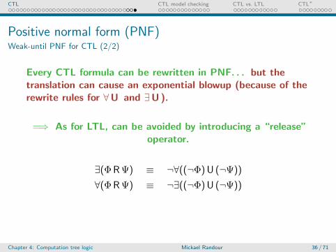
Every CTL formula can be rewritten in PNF. . . but thetranslation can cause an exponential blowup (because of therewrite rules for ∀U and ∃U ).
=⇒ As for LTL, can be avoided by introducing a “release”operator.
∃(ΦRΨ) ≡ ¬∀((¬Φ) U (¬Ψ))
∀(ΦRΨ) ≡ ¬∃((¬Φ) U (¬Ψ))
Chapter 4: Computation tree logic Mickael Randour 36 / 71
CTL CTL model checking CTL vs. LTL CTL∗
1 CTL: a specification language for BT properties
2 CTL model checking
3 CTL vs. LTL
4 CTL∗
Chapter 4: Computation tree logic Mickael Randour 37 / 71
CTL CTL model checking CTL vs. LTL CTL∗
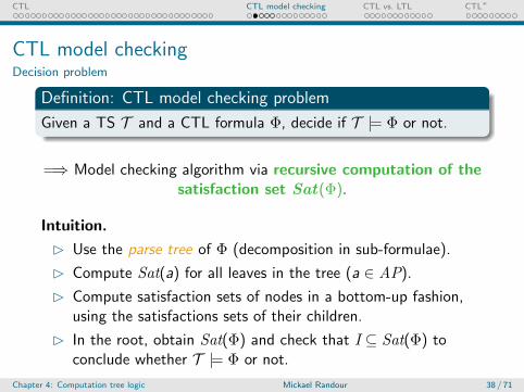
CTL model checkingDecision problem
Definition: CTL model checking problem
Given a TS T and a CTL formula Φ, decide if T |= Φ or not.
=⇒ Model checking algorithm via recursive computation of thesatisfaction set Sat(Φ).
Intuition.
� Use the parse tree of Φ (decomposition in sub-formulae).
� Compute Sat(a) for all leaves in the tree (a ∈ AP).
� Compute satisfaction sets of nodes in a bottom-up fashion,using the satisfactions sets of their children.
� In the root, obtain Sat(Φ) and check that I ⊆ Sat(Φ) toconclude whether T |= Φ or not.
Chapter 4: Computation tree logic Mickael Randour 38 / 71
CTL CTL model checking CTL vs. LTL CTL∗
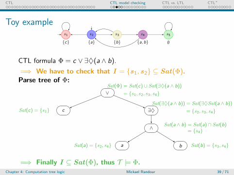
Toy examples1 s2 s3 s4 s5
{c} {a} {b} {a, b} ∅
CTL formula Φ = c ∨ ∃♦(a ∧ b).
=⇒ We have to check that I = {s1, s2} ⊆ Sat(Φ).Parse tree of Φ:
∨
c ∃♦
∧
a b
Sat(c) = {s1}
Sat(a) = {s2, s4} Sat(b) = {s3, s4}
Sat(a ∧ b) = Sat(a) ∩ Sat(b)= {s4}
Sat(∃♦(a ∧ b)) = Sat(∃♦Sat(a ∧ b))
= {s2, s3, s4}
Sat(Φ) = Sat(c) ∪ Sat(∃♦(a ∧ b))
= {s1, s2, s3, s4}
=⇒ Finally I ⊆ Sat(Φ), thus T |= Φ.Chapter 4: Computation tree logic Mickael Randour 39 / 71

CTL CTL model checking CTL vs. LTL CTL∗
Formulae in ENFThroughout this section, we assume formulae are written in ENF.
Reminder: ENF for CTL
Given atomic propositions AP, CTL formulae in existential normalform are given by:
Φ ::= true | a | Φ ∧Ψ | ¬Φ | ∃© Φ | ∃(ΦUΨ) | ∃�Φ
where a ∈ AP.
Assume we have Sat(Φ) and Sat(Ψ), we need algorithms for:
Sat(Φ∧Ψ) and Sat(¬Φ): easy, intersection and complement.
Sat(∃© Φ), Sat(∃(ΦUΨ)) and Sat(∃�Φ).
In practice, one can either rewrite any formula in ENF (but with apotential blow-up), or design specific algorithms to deal with ∀quantifiers (based on similar ideas).
Chapter 4: Computation tree logic Mickael Randour 40 / 71
CTL CTL model checking CTL vs. LTL CTL∗
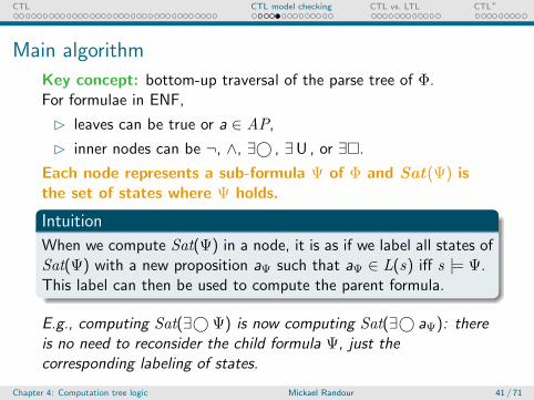
Main algorithm
Key concept: bottom-up traversal of the parse tree of Φ.For formulae in ENF,
� leaves can be true or a ∈ AP,
� inner nodes can be ¬, ∧, ∃© , ∃U , or ∃�.
Each node represents a sub-formula Ψ of Φ and Sat(Ψ) isthe set of states where Ψ holds.
Intuition
When we compute Sat(Ψ) in a node, it is as if we label all states ofSat(Ψ) with a new proposition aΨ such that aΨ ∈ L(s) iff s |= Ψ.This label can then be used to compute the parent formula.
E.g., computing Sat(∃©Ψ) is now computing Sat(∃© aΨ): thereis no need to reconsider the child formula Ψ, just thecorresponding labeling of states.
Chapter 4: Computation tree logic Mickael Randour 41 / 71
CTL CTL model checking CTL vs. LTL CTL∗
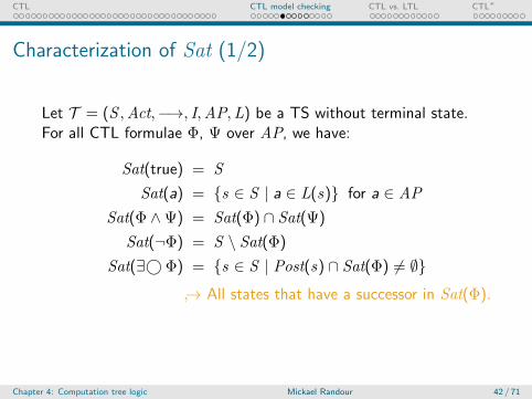
Characterization of Sat (1/2)
Let T = (S ,Act,−→, I,AP,L) be a TS without terminal state.For all CTL formulae Φ, Ψ over AP, we have:
Sat(true) = S
Sat(a) = {s ∈ S | a ∈ L(s)} for a ∈ AP
Sat(Φ ∧Ψ) = Sat(Φ) ∩ Sat(Ψ)
Sat(¬Φ) = S \ Sat(Φ)
Sat(∃© Φ) = {s ∈ S | Post(s) ∩ Sat(Φ) 6= ∅}
↪→ All states that have a successor in Sat(Φ).
Chapter 4: Computation tree logic Mickael Randour 42 / 71
CTL CTL model checking CTL vs. LTL CTL∗
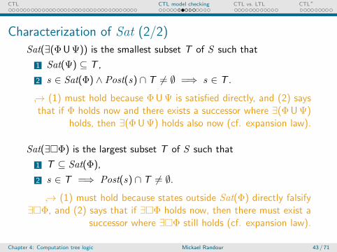
Characterization of Sat (2/2)
Sat(∃(ΦUΨ)) is the smallest subset T of S such that
1 Sat(Ψ) ⊆ T ,
2 s ∈ Sat(Φ) ∧ Post(s) ∩ T 6= ∅ =⇒ s ∈ T .
↪→ (1) must hold because ΦUΨ is satisfied directly, and (2) saysthat if Φ holds now and there exists a successor where ∃(ΦUΨ)
holds, then ∃(ΦUΨ) holds also now (cf. expansion law).
Sat(∃�Φ) is the largest subset T of S such that
1 T ⊆ Sat(Φ),
2 s ∈ T =⇒ Post(s) ∩ T 6= ∅.
↪→ (1) must hold because states outside Sat(Φ) directly falsify∃�Φ, and (2) says that if ∃�Φ holds now, then there must exist a
successor where ∃�Φ still holds (cf. expansion law).
Chapter 4: Computation tree logic Mickael Randour 43 / 71

CTL CTL model checking CTL vs. LTL CTL∗
Computation of Sat: algorithm (1/3)
Input: TS T = (S ,Act,−→, I,AP,L) and CTL formula Φ in ENFOutput: Sat(Φ) = {s ∈ S | s |= Φ}
if Φ = true thenreturn S
else if Φ = a ∈ AP thenreturn {s ∈ S | a ∈ L(s)}
else if Φ = Ψ1 ∧Ψ2 thenreturn Sat(Ψ1) ∩ Sat(Ψ2)
else if Φ = ¬Ψ thenreturn S \ Sat(Ψ)
else if Φ = ∃©Ψ thenreturn {s ∈ S | Post(s) ∩ Sat(Ψ) 6= ∅}
...
Chapter 4: Computation tree logic Mickael Randour 44 / 71
CTL CTL model checking CTL vs. LTL CTL∗
Computation of Sat: algorithm (2/3)
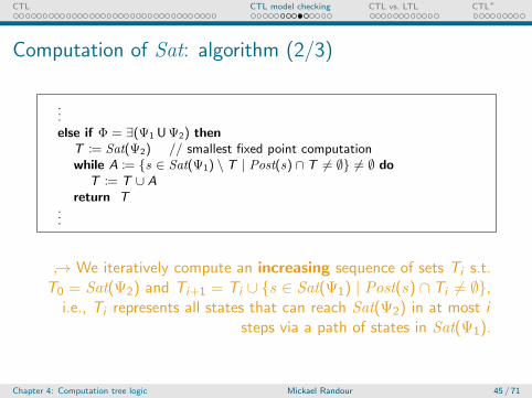
...else if Φ = ∃(Ψ1 UΨ2) then
T := Sat(Ψ2) // smallest fixed point computationwhile A := {s ∈ Sat(Ψ1) \ T | Post(s) ∩ T 6= ∅} 6= ∅ do
T := T ∪ Areturn T
...
↪→ We iteratively compute an increasing sequence of sets Ti s.t.T0 = Sat(Ψ2) and Ti+1 = Ti ∪ {s ∈ Sat(Ψ1) | Post(s) ∩ Ti 6= ∅},
i.e., Ti represents all states that can reach Sat(Ψ2) in at most isteps via a path of states in Sat(Ψ1).
Chapter 4: Computation tree logic Mickael Randour 45 / 71
CTL CTL model checking CTL vs. LTL CTL∗
Computation of Sat: algorithm (3/3)
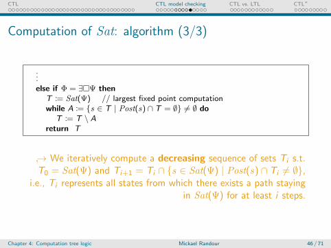
...else if Φ = ∃�Ψ then
T := Sat(Ψ) // largest fixed point computationwhile A := {s ∈ T | Post(s) ∩ T = ∅} 6= ∅ do
T := T \ Areturn T
↪→ We iteratively compute a decreasing sequence of sets Ti s.t.T0 = Sat(Ψ) and Ti+1 = Ti ∩ {s ∈ Sat(Ψ) | Post(s) ∩ Ti 6= ∅},
i.e., Ti represents all states from which there exists a path stayingin Sat(Ψ) for at least i steps.
Chapter 4: Computation tree logic Mickael Randour 46 / 71
CTL CTL model checking CTL vs. LTL CTL∗
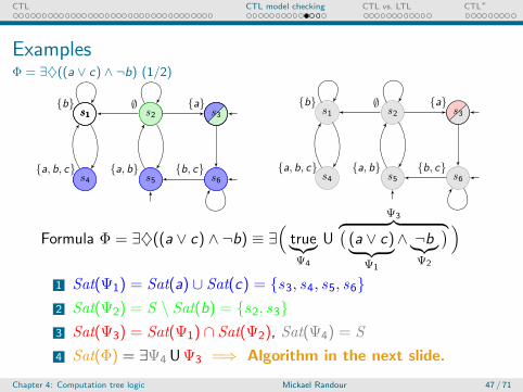
ExamplesΦ = ∃♦((a ∨ c) ∧ ¬b) (1/2)
s1 s2 s3
s4 s5 s6
s1 s2 s3
s4 s5 s6
s1 s2 s3
s4 s5 s6
{b} ∅ {a}
{a, b, c} {a, b} {b, c}
s1 s2 s3
s4 s5 s6
{b} ∅ {a}
{a, b, c} {a, b} {b, c}
Formula Φ = ∃♦((a ∨ c) ∧ ¬b) ≡ ∃(
true︸︷︷︸Ψ4
U
Ψ3︷ ︸︸ ︷((a ∨ c)︸ ︷︷ ︸
Ψ1
∧ ¬b︸︷︷︸Ψ2
) )1 Sat(Ψ1) = Sat(a) ∪ Sat(c) = {s3, s4, s5, s6}2 Sat(Ψ2) = S \ Sat(b) = {s2, s3}3 Sat(Ψ3) = Sat(Ψ1) ∩ Sat(Ψ2), Sat(Ψ4) = S
4 Sat(Φ) = ∃Ψ4 UΨ3 =⇒ Algorithm in the next slide.
Chapter 4: Computation tree logic Mickael Randour 47 / 71

CTL CTL model checking CTL vs. LTL CTL∗
ExamplesΦ = ∃♦((a ∨ c) ∧ ¬b) (2/2)
s1 s2s2 s3s3
s4 s5s5 s6s6
{b} ∅ {a}
{a, b, c} {a, b} {b, c}
We obtain Sat(Φ) = ∃Ψ4 UΨ3 via smallest fixed pointcomputation:
� T0 = Sat(Ψ3) = {s3}� T1 = T0 ∪ {s ∈ Sat(Ψ4) | Post(s) ∩ T0 6= ∅} = {s2, s3}� T2 = T1 ∪ {s ∈ Sat(Ψ4) | Post(s) ∩ T1 6= ∅} = {s2, s3, s5}� T3 = T2 ∪{s ∈ Sat(Ψ4) | Post(s)∩T2 6= ∅} = {s2, s3, s5, s6}� T4 = T3 ∪ {s ∈ Sat(Ψ4) | Post(s) ∩ T3 6= ∅} = T3 = Sat(Φ)
I = {s3, s5, s6} ⊆ Sat(Φ) =⇒ T |= Φ = ∃♦((a ∨ c) ∧ ¬b)Chapter 4: Computation tree logic Mickael Randour 48 / 71
CTL CTL model checking CTL vs. LTL CTL∗
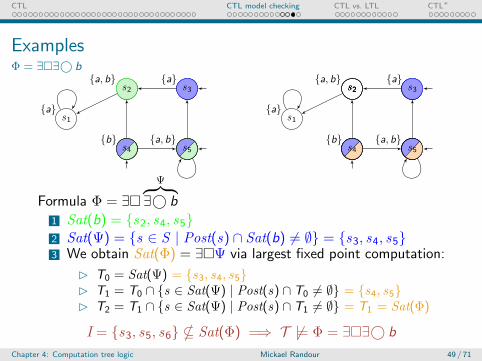
ExamplesΦ = ∃�∃© b
s1
s2 s3
s4 s5
s2 s3
s4 s5
s2 s3
s4 s5
{a}
{a, b} {a}
{b} {a, b}
s1
s2 s3
s4 s5
s2 s3
s4 s5
s2 s3
s4 s5
{a}
{a, b} {a}
{b} {a, b}
Formula Φ = ∃�Ψ︷ ︸︸ ︷∃© b
1 Sat(b) = {s2, s4, s5}2 Sat(Ψ) = {s ∈ S | Post(s) ∩ Sat(b) 6= ∅} = {s3, s4, s5}3 We obtain Sat(Φ) = ∃�Ψ via largest fixed point computation:
� T0 = Sat(Ψ) = {s3, s4, s5}� T1 = T0 ∩ {s ∈ Sat(Ψ) | Post(s) ∩ T0 6= ∅} = {s4, s5}� T2 = T1 ∩ {s ∈ Sat(Ψ) | Post(s) ∩ T1 6= ∅} = T1 = Sat(Φ)
I = {s3, s5, s6} * Sat(Φ) =⇒ T 6|= Φ = ∃�∃© b
Chapter 4: Computation tree logic Mickael Randour 49 / 71

CTL CTL model checking CTL vs. LTL CTL∗
Complexity of CTL model checkingClever implementations of algorithms for ∃(Ψ1 UΨ2) and∃�Ψ take time O(|S |+ | −→ |).
=⇒ See the book for detailed algorithms.
Main algorithm to compute Sat(Φ) is a bottom-up traversalof the parse tree: O(|Φ|).
Complexity of the algorithm
The time complexity is O(|T | · |Φ|).
=⇒ CTL model checking is in polynomial time!
=⇒ So. . . much more efficient than LTL which isPSPACE-complete?
=⇒ Not really. . . need to consider the whole picture,including succinctness!
Chapter 4: Computation tree logic Mickael Randour 50 / 71
CTL CTL model checking CTL vs. LTL CTL∗
1 CTL: a specification language for BT properties
2 CTL model checking
3 CTL vs. LTL
4 CTL∗
Chapter 4: Computation tree logic Mickael Randour 51 / 71
CTL CTL model checking CTL vs. LTL CTL∗
ExpressivenessIncomparable logics
We have seen that:
some properties are expressible in LTL but not in CTL (e.g.,φ = ♦�a),
some properties are expressible in CTL but not in LTL (e.g.,Φ = ∀�∃♦a),
some properties can be expressed in both logics (e.g.,φ = �♦a is equivalent to Φ = ∀�∀♦a).
LTL CTL
Can we characterize the intersection?
Chapter 4: Computation tree logic Mickael Randour 52 / 71
CTL CTL model checking CTL vs. LTL CTL∗
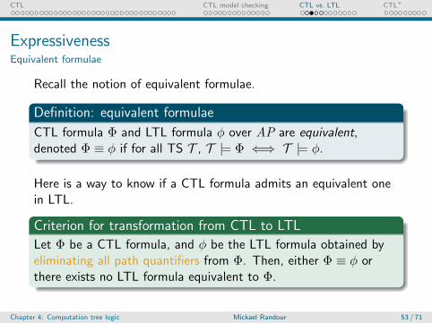
ExpressivenessEquivalent formulae
Recall the notion of equivalent formulae.
Definition: equivalent formulae
CTL formula Φ and LTL formula φ over AP are equivalent,denoted Φ ≡ φ if for all TS T , T |= Φ ⇐⇒ T |= φ.
Here is a way to know if a CTL formula admits an equivalent onein LTL.
Criterion for transformation from CTL to LTL
Let Φ be a CTL formula, and φ be the LTL formula obtained byeliminating all path quantifiers from Φ. Then, either Φ ≡ φ orthere exists no LTL formula equivalent to Φ.
Chapter 4: Computation tree logic Mickael Randour 53 / 71
CTL CTL model checking CTL vs. LTL CTL∗
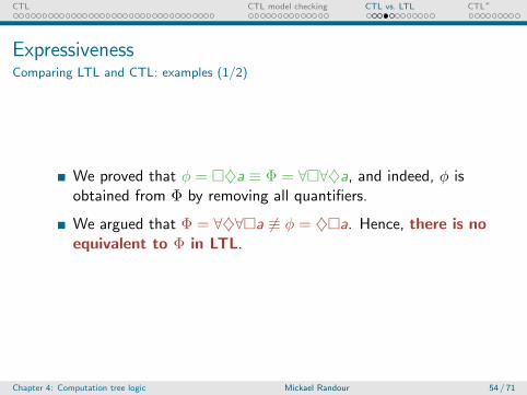
ExpressivenessComparing LTL and CTL: examples (1/2)
We proved that φ = �♦a ≡ Φ = ∀�∀♦a, and indeed, φ isobtained from Φ by removing all quantifiers.
We argued that Φ = ∀♦∀�a 6≡ φ = ♦�a. Hence, there is noequivalent to Φ in LTL.
Chapter 4: Computation tree logic Mickael Randour 54 / 71
CTL CTL model checking CTL vs. LTL CTL∗
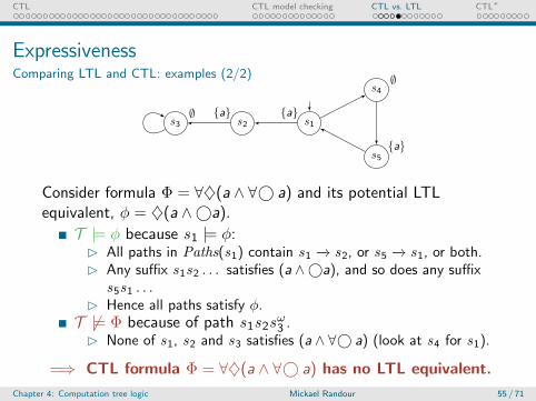
ExpressivenessComparing LTL and CTL: examples (2/2)
s1s2s3
s4
s5
{a}{a}∅
∅
{a}
Consider formula Φ = ∀♦(a ∧ ∀© a) and its potential LTLequivalent, φ = ♦(a ∧©a).
T |= φ because s1 |= φ:� All paths in Paths(s1) contain s1 −→ s2, or s5 −→ s1, or both.� Any suffix s1s2 . . . satisfies (a ∧©a), and so does any suffix
s5s1 . . .� Hence all paths satisfy φ.T 6|= Φ because of path s1s2s
ω3 .
� None of s1, s2 and s3 satisfies (a ∧ ∀© a) (look at s4 for s1).
=⇒ CTL formula Φ = ∀♦(a ∧ ∀© a) has no LTL equivalent.
Chapter 4: Computation tree logic Mickael Randour 55 / 71
CTL CTL model checking CTL vs. LTL CTL∗
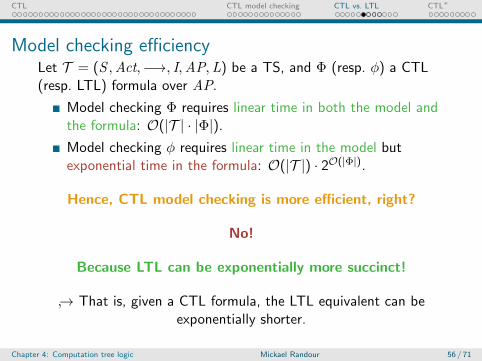
Model checking efficiencyLet T = (S ,Act,−→, I,AP,L) be a TS, and Φ (resp. φ) a CTL(resp. LTL) formula over AP.
Model checking Φ requires linear time in both the model andthe formula: O(|T | · |Φ|).
Model checking φ requires linear time in the model butexponential time in the formula: O(|T |) · 2O(|Φ|).
Hence, CTL model checking is more efficient, right?
No!
Because LTL can be exponentially more succinct!
↪→ That is, given a CTL formula, the LTL equivalent can beexponentially shorter.
Chapter 4: Computation tree logic Mickael Randour 56 / 71
CTL CTL model checking CTL vs. LTL CTL∗
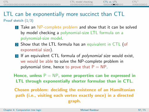
LTL can be exponentially more succinct than CTLProof sketch (1/3)
1 Take an NP-complete problem and show that it can be solvedby model checking a polynomial-size LTL formula on apolynomial-size model.
2 Show that the LTL formula has an equivalent in CTL (ofexponential size).
3 If an equivalent CTL formula of polynomial size would exist,we would be able to solve the NP-complete problem inpolynomial time, hence to prove that P = NP.
Hence, unless P = NP, some properties can be expressed inLTL through exponentially shorter formulae than in CTL.
Chosen problem: deciding the existence of an Hamiltonianpath (i.e., visiting each vertex exactly once) in a directed
graph.
Chapter 4: Computation tree logic Mickael Randour 57 / 71
CTL CTL model checking CTL vs. LTL CTL∗
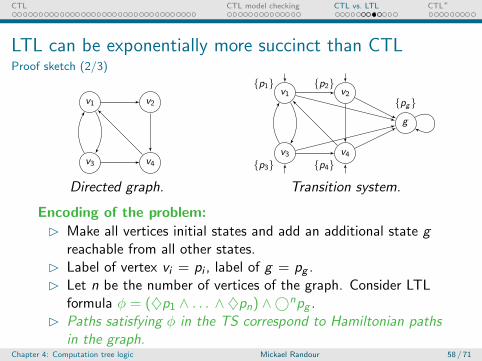
LTL can be exponentially more succinct than CTLProof sketch (2/3)
v1 v2
v3 v4
Directed graph.
v1 v2
v3 v4
g
{p1} {p2}
{p3} {p4}
{pg}
Transition system.
Encoding of the problem:
� Make all vertices initial states and add an additional state greachable from all other states.
� Label of vertex vi = pi , label of g = pg .� Let n be the number of vertices of the graph. Consider LTL
formula φ = (♦p1 ∧ . . . ∧ ♦pn) ∧©npg .� Paths satisfying φ in the TS correspond to Hamiltonian paths
in the graph.Chapter 4: Computation tree logic Mickael Randour 58 / 71
CTL CTL model checking CTL vs. LTL CTL∗
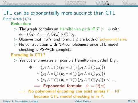
LTL can be exponentially more succinct than CTLProof sketch (3/3)
Reduction:
� The graph contains an Hamiltonian path iff T 6|= ¬φ withφ = (♦p1 ∧ . . . ∧ ♦pn) ∧©npg .
� Observe that TS T and formula φ are both of polynomial size.� No contradiction with NP-completeness since LTL model
checking is PSPACE-complete.
Encoding in CTL?
� Yes but enumerates all possible Hamiltonian paths! E.g.,
Φ = (p1 ∧ ∃© (p2 ∧ ∃© (p3 ∧ ∃© p4)))
∨ (p1 ∧ ∃© (p2 ∧ ∃© (p4 ∧ ∃© p3)))
∨ (p1 ∧ ∃© (p3 ∧ ∃© (p2 ∧ ∃© p4))) ∨ . . .
=⇒ Exponential formula: |Φ| = O(n!)
=⇒ No polynomial encoding can exist unless P = NPbecause CTL model checking is in P.
Chapter 4: Computation tree logic Mickael Randour 59 / 71
CTL CTL model checking CTL vs. LTL CTL∗
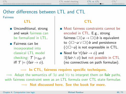
Other differences between LTL and CTLFairness
LTL
Unconditional, strongand weak fairness canbe formalized in LTL.
Fairness can beincorporated intoclassical LTL modelchecking: T |=fair φiff T |= (fair→ φ).
CTL
Most fairness constraints cannot beencoded in CTL. E.g., strongfairness �♦a→ �♦b is equivalentto ♦�¬a ∨�♦b and persistence(♦�¬a) is not expressible in CTL.
Need for ∀(fair→ φ) and∃(fair ∧ φ) but not possible in CTL(no connectives on path formulae).
=⇒ In CTL, fairness requires specific techniques.
=⇒ Adapt the semantics of ∃φ and ∀φ to interpret them on fair paths,with fairness constraint seen as an LTL formula over CTL state formulae.
=⇒ Not discussed here. See the book for more.
Chapter 4: Computation tree logic Mickael Randour 60 / 71

CTL CTL model checking CTL vs. LTL CTL∗
Other differences between LTL and CTLImplementation relation
LTL
LTL is preserved by traceinclusion (PSPACE-c.).
(Bi)simulation is a soundbut incomplete alternative,computable in polynomialtime.
(bi)simulation⇓ 6⇑
trace inclusion
CTL
Bisimulation preserves fullCTL.
Simulation preserves theuniversal fragment of CTL.
↪→ Allows only quantifier ∀.
Equivalently, simulationpreserves the existentialfragment of CTL.
↪→ Allows only quantifier ∃(recall ∀φ ≡ ¬∃¬φ).
=⇒ Different logics, different implementation relations.
Chapter 4: Computation tree logic Mickael Randour 61 / 71
CTL CTL model checking CTL vs. LTL CTL∗
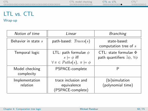
LTL vs. CTLWrap-up
Notion of time Linear Branching
Behavior in state s path-based: Traces(s) state-based:computation tree of s
Temporal logic LTL: path formulae φs |= φ iff
∀π ∈ Paths(s), π |= φ
CTL: state formulae Φpath quantifiers ∃φ, ∀φ
Model checkingcomplexity
PSPACE-complete P
Implementationrelation
trace inclusion andequivalence
(PSPACE-complete)
(bi)simulation(polynomial time)
Chapter 4: Computation tree logic Mickael Randour 62 / 71
CTL CTL model checking CTL vs. LTL CTL∗
1 CTL: a specification language for BT properties
2 CTL model checking
3 CTL vs. LTL
4 CTL∗
Chapter 4: Computation tree logic Mickael Randour 63 / 71
CTL CTL model checking CTL vs. LTL CTL∗
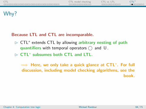
Why?
Because LTL and CTL are incomparable.
� CTL∗ extends CTL by allowing arbitrary nesting of pathquantifiers with temporal operators © and U .
� CTL∗ subsumes both CTL and LTL.
=⇒ Here, we only take a quick glance at CTL∗. For fulldiscussion, including model checking algorithms, see the
book.
Chapter 4: Computation tree logic Mickael Randour 64 / 71
CTL CTL model checking CTL vs. LTL CTL∗
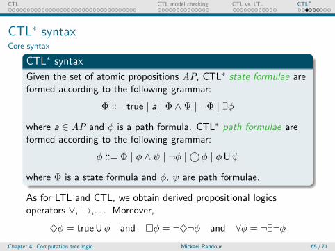
CTL∗ syntaxCore syntax
CTL∗ syntax
Given the set of atomic propositions AP, CTL∗ state formulae areformed according to the following grammar:
Φ ::= true | a | Φ ∧Ψ | ¬Φ | ∃φ
where a ∈ AP and φ is a path formula. CTL∗ path formulae areformed according to the following grammar:
φ ::= Φ | φ ∧ ψ | ¬φ | ©φ | φUψ
where Φ is a state formula and φ, ψ are path formulae.
As for LTL and CTL, we obtain derived propositional logicsoperators ∨, →,. . . Moreover,
♦φ = true Uφ and �φ = ¬♦¬φ and ∀φ = ¬∃¬φChapter 4: Computation tree logic Mickael Randour 65 / 71

CTL CTL model checking CTL vs. LTL CTL∗
CTL∗ syntaxExamples (1/2)
CTL∗ syntax reminder
Φ ::= true | a | Φ∧Ψ | ¬Φ | ∃φ φ ::= Φ | φ∧ψ | ¬φ | ©φ | φUψ
Is Φ = ∃©a a valid CTL∗ formula? (yes for CTL)
� Yes, because φ =©a is a valid path formula, hence Φ = ∃φ isa valid state formula.
Is Φ = a ∧ b a valid CTL∗ formula? (yes for CTL)
� Yes, because Ψ1 = a and Ψ2 = b are valid state formulae,hence Φ = Ψ1 ∧Ψ2 is a valid state formula.
Is Φ = ∀(a ∧ ∃© b) a valid CTL∗ formula? (no for CTL)
� Yes, because Ψ = a ∧ ∃© b is a valid state formula and anystate formula Ψ can be taken as a path formula φ = Ψ.
Chapter 4: Computation tree logic Mickael Randour 66 / 71
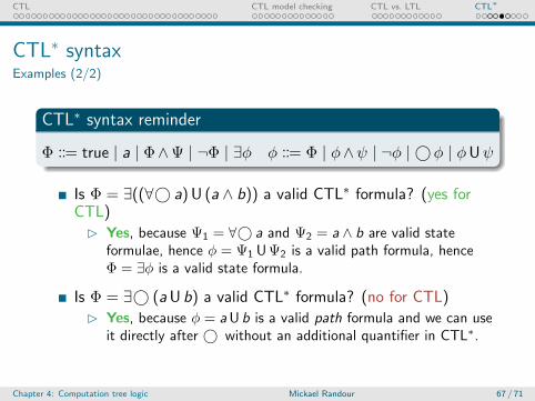
CTL CTL model checking CTL vs. LTL CTL∗
CTL∗ syntaxExamples (2/2)
CTL∗ syntax reminder
Φ ::= true | a | Φ∧Ψ | ¬Φ | ∃φ φ ::= Φ | φ∧ψ | ¬φ | ©φ | φUψ
Is Φ = ∃((∀© a) U (a ∧ b)) a valid CTL∗ formula? (yes forCTL)
� Yes, because Ψ1 = ∀© a and Ψ2 = a ∧ b are valid stateformulae, hence φ = Ψ1 UΨ2 is a valid path formula, henceΦ = ∃φ is a valid state formula.
Is Φ = ∃© (aU b) a valid CTL∗ formula? (no for CTL)
� Yes, because φ = aU b is a valid path formula and we can useit directly after © without an additional quantifier in CTL∗.
Chapter 4: Computation tree logic Mickael Randour 67 / 71

CTL CTL model checking CTL vs. LTL CTL∗
Semantics
The semantics of CTL∗ follows naturally from the one of CTL.
Chapter 4: Computation tree logic Mickael Randour 68 / 71

CTL CTL model checking CTL vs. LTL CTL∗
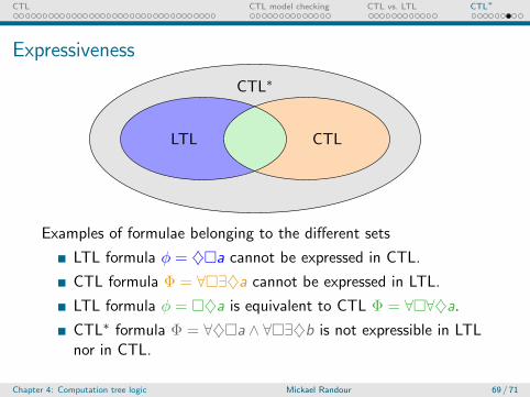
Expressiveness
LTL CTL
CTL∗
Any CTL formula is also a CTL∗ formula.� Indeed, the syntax of CTL is a subset of the one of CTL∗.
Any LTL formula φ has an equivalent CTL∗ formula.� We have T |= φ ⇐⇒ T |= Φ = ∀φ.
=⇒ CTL∗ is strictly more expressive than LTL and CTL,i.e., there exist CTL∗ formulae that cannot be expressed
neither in LTL nor in CTL.
Chapter 4: Computation tree logic Mickael Randour 69 / 71
CTL CTL model checking CTL vs. LTL CTL∗
Expressiveness
LTL CTL
CTL∗
Examples of formulae belonging to the different sets
LTL formula φ = ♦�a cannot be expressed in CTL.
CTL formula Φ = ∀�∃♦a cannot be expressed in LTL.
LTL formula φ = �♦a is equivalent to CTL Φ = ∀�∀♦a.
CTL∗ formula Φ = ∀♦�a ∧ ∀�∃♦b is not expressible in LTLnor in CTL.
Chapter 4: Computation tree logic Mickael Randour 69 / 71
CTL CTL model checking CTL vs. LTL CTL∗
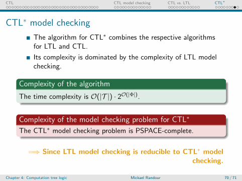
CTL∗ model checking
The algorithm for CTL∗ combines the respective algorithmsfor LTL and CTL.
Its complexity is dominated by the complexity of LTL modelchecking.
Complexity of the algorithm
The time complexity is O(|T |) · 2O(|Φ|).
Complexity of the model checking problem for CTL∗
The CTL∗ model checking problem is PSPACE-complete.
=⇒ Since LTL model checking is reducible to CTL∗ modelchecking.
Chapter 4: Computation tree logic Mickael Randour 70 / 71
CTL CTL model checking CTL vs. LTL CTL∗
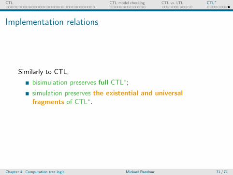
Implementation relations
Similarly to CTL,
bisimulation preserves full CTL∗;
simulation preserves the existential and universalfragments of CTL∗.
Chapter 4: Computation tree logic Mickael Randour 71 / 71
References I
C. Baier and J.-P. Katoen.
Principles of model checking.MIT Press, 2008.
Chapter 4: Computation tree logic Mickael Randour 72 / 71