CHAPTER 4 Composite Dielectric Materialsdl.iran-mavad.com/sell/trans/en/Composite Dielectric...
23
CHAPTER 4 Composite Dielectric Materials 4.1 Introduction Composite dielectrics represent, in general, a heterogeneous system of multiconstituent materials. Typically, a two-phase composite dielectric is constituted by a host material with an inclusion of another material. This host-inclusion system could be formed by a combination (or a mixture) of dielectric-dielectric, dielectric-conductor, and/or dielectric-semiconductor phases. The constituent phases may form structurally an embedment system consisting of multi-layer "layups" or random dispersion of the inclusions across the host medium; or there could be a structured matrix of specific type to yield certain desirable dielectric properties. Generically, a composite dielectric can be treated as as a mixture-medium, largely heterogeneous and could be anisotropic and nonlinear, as well. 4.2 Theory of Dielectric Mixtures Mixture models describing the effective response of dielectric mixtures to electromagnetic stimulus have been addressed comprehensively in the literature [1]. Such mixtures are useful in several electromagnetic applications. Radar absorbing materials (RAMs), surface coatings non-reflective to electromagnetic waves, electrostatic dissipative compounds, EM! shielding materials, special purpose insulators, bioelectromagnetic phantoms, and conductive adhesives used in microelectronics are a few examples of composite dielectrics. A dielectric mixture can be synthesized in a number of ways. Typically the following are the host-inclusion systems considered in the dielectric mixture theory: • SphericaVnear-spherical inclusions dispersed randomly as "chunks" in a homogeneous host medium • Elongated (ellipsoidal or spheroidal) inclusions dispersed randomly in a homogeneous receptacle • Fibrous (needle-like) inclusions with random dispositions in the host medium • Random dispersion of flaky (disk-like) inclusions in the host medium • Multi-layer of laminates or orderly "stacked-up" individual laminae (of different phases) • Orderly-oriented and laid stretches ("tows'') of fibers in a host medium • Special geometrical inclusions (such as honey-comb, mesh-like structures) embedded in the host • Multiphase composite with voids/porosity introduced deliberately However, irrespective of the shape, size, physical state, volume fraction, or orientation of different phases, the effective dielectric response of the mixture and hence its constitutive dielectric parameter, namely, the effective permittivity (eejJ)' should always lie within two specified limits referred to as the Wiener bounds which will be discussed in detail in a later section. In the following section, general considerations of dielectric mixture theory [1] pertinent to the foregoing types of dielectric mixtures are reviewed and state-of-the-art models describing the effective permittivity are addressed. Even in the case of the simplest type of 105
Transcript of CHAPTER 4 Composite Dielectric Materialsdl.iran-mavad.com/sell/trans/en/Composite Dielectric...
CHAPTER 4
Composite Dielectric Materials
4.1 Introduction Composite dielectrics represent, in general, a heterogeneous system of
multiconstituent materials. Typically, a two-phase composite dielectric is constituted by a host material with an inclusion of another material. This host-inclusion system could be formed by a combination (or a mixture) of dielectric-dielectric, dielectric-conductor, and/or dielectric-semiconductor phases. The constituent phases may form structurally an embedment system consisting of multi-layer "layups" or random dispersion of the inclusions across the host medium; or there could be a structured matrix of specific type to yield certain desirable dielectric properties. Generically, a composite dielectric can be treated as as a mixture-medium, largely heterogeneous and could be anisotropic and nonlinear, as well.
4.2 Theory of Dielectric Mixtures Mixture models describing the effective response of dielectric mixtures to
electromagnetic stimulus have been addressed comprehensively in the literature [1]. Such mixtures are useful in several electromagnetic applications. Radar absorbing materials (RAMs), surface coatings non-reflective to electromagnetic waves, electrostatic dissipative compounds, EM! shielding materials, special purpose insulators, bioelectromagnetic phantoms, and conductive adhesives used in microelectronics are a few examples of composite dielectrics.
A dielectric mixture can be synthesized in a number of ways. Typically the following are the host-inclusion systems considered in the dielectric mixture theory:
• SphericaVnear-spherical inclusions dispersed randomly as "chunks" in a homogeneous host medium
• Elongated (ellipsoidal or spheroidal) inclusions dispersed randomly in a homogeneous receptacle
• Fibrous (needle-like) inclusions with random dispositions in the host medium
• Random dispersion of flaky (disk-like) inclusions in the host medium
• Multi-layer of laminates or orderly "stacked-up" individual laminae (of different phases)
• Orderly-oriented and laid stretches ("tows'') of fibers in a host medium
• Special geometrical inclusions (such as honey-comb, mesh-like structures) embedded in the host
• Multiphase composite with voids/porosity introduced deliberately
However, irrespective of the shape, size, physical state, volume fraction, or orientation of different phases, the effective dielectric response of the mixture and hence its constitutive dielectric parameter, namely, the effective permittivity (eejJ)' should always lie within two specified limits referred to as the Wiener bounds which will be discussed in detail in a later section.
In the following section, general considerations of dielectric mixture theory [1] pertinent to the foregoing types of dielectric mixtures are reviewed and state-of-the-art models describing the effective permittivity are addressed. Even in the case of the simplest type of
105
106 Handbook of Electromagnetic Materials
mixtures with two constitutive phases, it is indicated that the dielectric characteristics are dependent not only on the dielectric polarizabiIity of the constituents but also the stochastic attributes of the mixture medium.
4.3 Permittivity of Heterogeneous Mixtures The earliest version of a dielectric model of a two-phase heterogeneous mixture is due
to Clausius and Mossotti [2], who on similar considerations of Maxwell-Garnett theory [3,4] (applied to conducting spherical particulates dispersed in a dielectric host medium) derived the following expression for the effective permittivity EejJof the mixture assuming that the constituents of the mixture are electrostatically noninteracting:
(4.1)
where E1 and EZ are the relative permittivities of the inclusions and the host medium, respectively, and 8 is the volume fraction of the inclusions. Equation 4.1 is popularly known as the Clausius-Mossotti formula [2] for the effective permittivity of a dielectric mixture.
In many cases, dielectric mixtures have more heterogeneous characteristics than the model potrayed by Clausius and Mossotti; and as such the dielectric formulations developed to describe many of such mixtures are empirical or semi-empirical in nature, decided by curve-fitting strategies to experimental data. However, rigorous formulations taking heterogeneity into account have also been developed by extending the binary phase model of Clausius and Mossotti. The following is the chronological account on the development of various dielectric mixture theories.
Following the Clausius-Mossotti approach, Rayleigh [5] obtained Equation (4.1) in another form for diluted dispersions (that is, for small volume fractions, 8« 1). It is given by:
(4.2)
Bruggeman [6] applied Rayleigh's formula to incremental changes in the volume loading of the composite medium sequentially and arrived at the so-called one-third power law, namely:
(4.3)
or, in the limiting case of IE11 « IEZI and I Ee!!1 , Equation 4.3 specifies that
EejJ == EZ( 1 - 8/12• An extension of Equation 4.3 written in the form EejJ = EZ( 1 - 8l
with d = 1 to 5 refers to Archie's law [7] widely used in studies on geophysical substances. The electrostatic-based mixture formulations on electrical capacity of dispersed systems
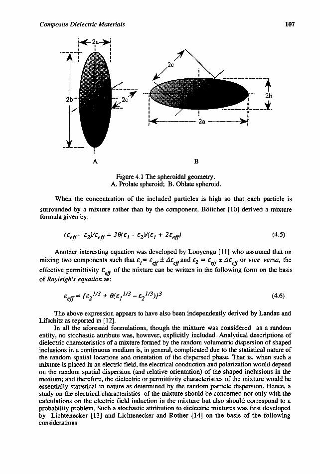
was extended by Fricke [8,9] to include a "shape-factor" in order to account for the particulate shape. Thus, Fricke's formula has an eccentricity term (x') based on the geometrical aspect of prolate and/or oblate spheroidal inclusions depicted in Figure 4.1. It is given by:
Composite Dielectric Materials 107
i~2a>: · .. ·······t I
A B
Figure 4.1 The spheroidal geometry. A. Prolate spheroid; B. Oblate spheroid.
When the concentration of the included particles is high so that each particle is
surrounded by a mixture rather than by the component, Bottcher [10] derived a mixture formula given by:
(4.5)
Another interesting equation was developed by Looyenga [11] who assumed that on mixing two components such that E1= Eeff± L1Eeffand E2 = Eeff:; fiEeff or vice versa, the
effective permittivity ceff of the mixture can be written in the following form on the basis
of Rayleigh's equation as:
(4.6)
The above expression appears to have also been independently derived by Landau and Lifschitz as reported in [12].
In all the aforesaid formulations, though the mixture was considered as a random entity, no stochastic attribute was, however, explicitly included. Analytical descriptions of dielectric characteristics of a mixture formed by the random volumetric dispersion of shaped inclusions in a continuous medium is, in general, complicated due to the statistical nature of the random spatial locations and orientation of the dispersed phase. That is, when such a mixture is placed in an electric field, the electrical conduction and polarization would depend on the random spatial dispersion (and relative orientation) of the shaped inclusions in the medium; and therefore, the dielectric or permittivity characteristics of the mixture would be essentially statistical in nature as determined by the random particle dispersion. Hence, a study on the electrical characteristics of the mixture should be concerned not only with the calculations on the electric field induction in the mixture but also should correspond to a probability problem. Such a stochastic attribution to dielectric mixtures was first developed by Lichtenecker [13] and Lichtenecker and Rother [14] on the basis of the following considerations.
108 Handbook of Electromagnetic Materials
Considering a two-component system in which the inclusions with a permittivity E]
are dispersed in a continuous medium of permittivity E2, the system can be regarded as a
matrix in which the dispersing medium represents a receptacle for the mutually isolated (or out-of-contact) particulate inclusions as indicated by Zheludev [15]. The effective permittivity (Eejf) of this matrix mixture would then depend on the permittivities of the mixture constituents, namely, E] and E2, and on the volume fraction (8) of the inclusions.
The function which interrelates Eel]' and other quantities, namely, E], E2 , and 8, would be determined both by electric field induction in the mixture as well as by the statistical considerations arising from random volumetric dispersion (and relative orientation) of the inclusions. Thus, the value of the effective permittivity of a statistical mixture can be described by a certain function F] as follows:
(4.7)
where q is aformfactor which depends on the shape of the inclusions. In the above equation (Equation 4.7), though a two-component case is considered, the discussion can be extended to any number of mixture components without any loss of generality. (Such multiphase systems are discussed in Chapter 6.)
All the theoretical works on the topic under discussion aim at finding the explicit nature of the function F] in Equation 4.7 and in the determination of this function, certain conditions have to be observed relevant to statistical mixtures. They are: (i) If the values of the permittivity of all the components of the mixture change in one and the same ratio, the value of the effective permittivity of the mixture (Eefj) should change identically (Wiener's
proportionality postulate [16]). Hence, F] must be a homogeneous function of the first degree extracted from the set of independent variables E] and E2• That is,
(4.8)
where s is an arbitrary constant factor. The above postulation follows directly from the laws of electrostatics according to which the direction of the lines of electric field at the boundary of two dielectrics depends only on the ratio of the permittivities of these dielectrics and is independent of their absolute values. (ii) The permittivity of a heterogeneous system (mixture) is closely connected with the arrangement of the particles in the system in relation to the field direction as can be seen from the simple example of a two-component laminated dielectric system shown in Figure (4.2). When the directions of the field and of the laminations coincide (parallel combination, Figure (4.2a), it follows that:
(4.9)
and when the field and lamination directions are perpendicular (series combination, Figure 4.2b), the following relation holds good:
(4.10)
The true value of the effective permittivity (Eejf) of a statistical mixture shown in
Figure (4.2c) should in fact, lie between the extreme values determined by Equations 4.9 and 4.10. Hence, it is constrained by the following inequalities suggested by Wiener in 1912 [16]:
Composite Dielectric Materials 109
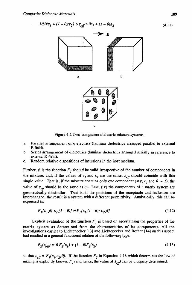
1/[O/E] + (1- OYE215 Eeff 5 OE] + (1- O)E2 (4.11)
~E
a b
c
Figure 4.2 Two-component dielectric mixture systems.
a. Parallel arrangement of dielectrics (laminar dielectrics arranged parallel to external E-field).
b. Series arrangement of dielectrics (laminar dielectrics arranged serially in reference to external E-field).
c. Random relative dispositions of inclusions in the host medium.
Further, (iii) the function F] should be valid irrespective of the number of components in
the mixture; and, if the values of E] and E2 are the same, Eeff should coincide with this single value. That is, if the mixture contains only one component (say, E] and 0 = 1), the
value of Eeff should be the same as Er Last, (iv) the components of a matrix system are geometrically dissimilar. That is, if the positions of the receptacle and inclusion are interchanged, the result is a system with a different permittivity. Analytically, this can be expressed as:
(4.12)
Explicit evaluation of the function F] is based on ascertaining the properties of the
matrix system as determined from the characteristics of its components. All the investigations earlier to Lichtenecker [13] and Lichtenecker and Rother [14] on this aspect had resulted in a general functional relation of the following type:
(4.13)
so that Eeff = F/E],E2,O). If the function F2 in Equation 4.13 which determines the law of mixing is explicitly known, F] (and hence, the value of Eeff) can be uniquely determined.
110 Handbook of Electromagnetic Materials
The analytical endeavor of evaluating the function F2 (or the function F j ) for various types of dielectric mixtures has resulted in several mixture relations and a comprehensive review of them was published by Brown [17] and by van Beek [18]. The contents of these reviews have also been summarized and reported by Tinga et al. [19]. These existing dielectric mixture formulations can be grouped into three major categories with the following characteristics: (i) Formulations based on electric field induction in the mixture containing spherical inclusions which either mutually interact or do not interact; (ii) analyses based on the electric field induction in the mixture containing shaped inclusions such as ellipsoids, oblate/prolate spheroids, needle-like, or disk-like particles, etc. and depolarization effects due to particle shape are either considered or ignored and; last (iii) formulations based on the theory of mixture which is regarded as a probability problem.
The investigations on dielectric mixtures due to Lorenz [20], Rayleigh [5], Bruggeman
[6], Bottcher [10], Meredith and Tobias [21], and Looyenga [11] fall under the first group cited above. Considering the second category, in which the particle shapes have been explicitly taken into account, the works of Wiener [16], Fricke [8,9], Sillars [22], Polder and Van Santen [23], Lewin [24], Hamon [25], Boned and Peyrelasse [26], and Sihvola and Kong [27] can be regarded as significant contributions.
However, studies dealing with the calculations (of the third type mentioned above) which are based on statistical considerations of the dielectric mixture are relatively few in number. In effect, reference can be made to only one work on the subject, that of Lichtenecker [13] who proposed the logarithmic law of mixing which can be summarized as follows.
Considering the theory of mixtures as a probability problem, Lichtenecker [13] and Lichtenecker and Rother [14] deduced the logarithmic mixture law from the general principles of statistics. For a mixture of two components, it is given by:
(-1~k~J) (4.14)
Here, where k = 1, Equation 4.14 gives the same expression for e eff as derived for a laminated dielectric (field parallel to the laminations, Figure 4.2a); and, for k = -1, Equation 4.14 gives the expression for a laminated dielectric (field perpendicular to the laminations, Figure 4.2b). For an unordered system k tends to zero and the formula of Equation 4.14 assumes the following form:
or
" -" 0" (J-e) Leff- L1 ~2 (4. 15a)
(4.15b)
Experimental studies on heterogeneous dielectric systems support Lichtenecker's formula even for anisotropic media such as barium titanate-polystyrol mixture as indicated by Zheludev [27]. The author [28] applied Lichtenecker's formula successfully to describe the complex permittivity of a poly crystalline (organic) compound taken in powder form and to evaluate the dielectric constant of human blood [29]. Wallin [30] indicated that the logarithmic law (or its modified versions) fits closely the experimental data on oil shale. On the basis of these results, a major conclusion is that the logarithmic law of mixing holds good at all volume fractions in describing the dielectric behavior (static or dynamic) of statistical mixtures. For spherical inclusions and also for almost sphere-like particles with uneven and coarse surfaces (as in the case of polycrystalline powder samples), the geometrical shape of the particles does not play a significant role in determining the macroscopic dielectric behavior of the mixture. That is, any small depolarization effects which may arise due to the relative orientation of coarsely surfaced (almost sphere-like)
Composite Dielectric Materials 111
particles are overwhelmed by the stochastic characterizations resulting from random dispersion of the inclusions in the volume of the mixture concerned. Hence, as depicted by Equation (4.15), the permittivity of such mixtures is solely a function of the permittivities and the relative volumes of the mixture constituents.
4.4 Dependence of Permittivity on Particulate Geometry Considering a dielectric mixture containing shapedlaspherical inclusions randomly
dispersed in the host, it is necessary to attribute a shape or a form factor to the particulates in question to account for the depolarization effects. The particles/inclusions are called shaped if two or more of the lateral dimensions of the particles are significantly different as in the case of ellipsoids, prolate/oblate spheroids, and disk-like or needle-like particles.
For a spheroidal geometry (Figure 4.1) with semiaxial lengths a, b, and c and taking b=c, the aspect ratio is equal to (alb). When this aspect ratio is of significant value (either large or small compared to unity) the corresponding eccentricity (e) would playa dominant role in the polarization of the particles when the mixture is subjected to an external field; and the depolarization arising from the relative disposition of the particles due to the random nature of particle dispersion (andlor orientation) in the mixture would become another effective stochastic parameter to be considered. As stated earlier, the works of Wiener [16], Fricke [8,9], Sillars [22], Lewin [24], and Hamon [25] are the earliest contributions which explicitly take into account the particle shape.
The logarithmic law per se does not contain any term to account for the particulate shape. Hence, it predicts the mixture permittivity as independent of the particulate shape and is applicable only to spherical/near-spherical inclusions. This drawback (the "shapeless" aspect) of the logarithmic law was criticized as inconsistent and theoretically unsound by Reynold and Hough [31] and later by Dukhin [32]. However, the author [33] obviated this deficiency of the logarithmic law by combining it with the well-known Fricke's formula thereby giving a modified version of the logarithmic law which explicitly accounts for the particle shape as explained below.
Fricke in his two classical papers [8,9] developed an expression for the effective permittivity of a dielectric mixture with an explicit shape/form factor to account for the shape of the inclusions. His analytical description of the mixture was based on the electric field induction in the dispersed system. The effective permittivity (Ee!!) of the mixture was expressed in terms of the permittivities of the host E2 and inclusions E]' the volume fraction (0) of the inclusions and a shape/form factor x'o to account for the depolarization effects in the electrical induction flux as:
(4.16)
where x'o' the shape/form factor is dependent on the ratio of EJlIE2• However, the results obtained on the basis of Fricke's formula deviated significantly from the measured data. Hence the author [33] included a statistical attribution to Fricke's formula on the basis of the logarithmic law to obtain a modified form factor Xo given by:
(4.17)
where M is a function of the (alb) ratio of the inclusions. Considering the particulate inclusions, they could in general either be oblate spheroidal
(a > b) or prolate spheroidal (a < b) as indicated in Figure (4.1). In the extreme cases (a < < b), they tend to be needles and for (a » b), they become disks. For an oblate spheroid, the eccentricity is given by e = (1 - b/a) and correspondingly for prolate spheroidal inclusions the eccentricity, e = (1 - alb). The factor M in the above equation (Equation 4.17) can be
112 Handbook of Electromagnetic Materials
expressed in tenns of the eccentricity of the inclusions as M = 2I(m-l) or (m-l)12 depending on whether e 1 ~ e2 or E 1 ::;; E2 , respectively; and the parameter m is related to the eccentricity e as follows [22]:
m = e2[J - (1- e2/ 12[arcsin (e)/e};-l (4.18)
The aforesaid modified version of the Fricke's fonnula as proposed in [33] has yielded results which correlate closely with the measured values pertaining to certain test mixtures.
Reynolds and Hough [31] succeeded in reducing all the existing mixture fonnulations except the logarithmic law to the generalized linear functional form of the type specified by Equation 4.13. In order to overcome this inconsistency pertaining to the logarithmic law, the author [34] also developed an improved version of the logarithmic law of mixing based on a weighted coefficient fonnat that fitted into a generalized linear fonn. Further, it had been generally contended that the logarithmic law could not be extended to a mixture with lossy dielectric and metallic (conductor) inclusions. On the contrary, the author successfully applied the logarithmic law to mixtures with conducting inclusions as elaborated in [35] on the basis of electrical susceptibility considerations as will be discussed in Chapter 6.
Inasmuch as the logarithmic law of mixing is not amenable for representation by a sample, generalized linear function, Reynolds and Hough [31] doubted some error in the logarithmic fonnulation and later (in 1974) Dukhin and Shilor [32] attributed the observed inconsistency to an illogical assumption by Lichtenecker [13] who considered a disperse system as chaotic and ordered simultaneously.
Despite the prevalence of the aforesaid mathematical inconsistency, the logarithmic law of mixing has surprisingly gained recognition, supported by experimental data gathered on stochastic mixtures with near-spherical inclusions [28,29]. As such it was considered preferable to eliminate the persisting incompatibility of the logarithmic law with respect to the generalized linear fonn. This has been done by the modifications as suggested by the author in [34] and is described below.
Considering a stochastic mixture, the effective pennittivity as given by the logarithmic law of mixing corresponds to a weighted geometrical mean of E1S and e2S' namely,
6 (1-6) Eeff = E2l1S .
The logarithmic relation can also be specified in a different form of weighted geometrical mean as presented below:
(4.19)
-1 where eu = 8E2 + (1 - 8)E1 and EL = [8/E2 + (J - 8)/E1) are Wiener's upper and lower limits, respectively (see Equations 4.9 and 4.10). In Equation 4.19, it is presumed that the nth fraction of the stochastic mixture system behaves as if polarized in the direction of the electric field induction and the remaining (1- nih fraction is polarized orthogonally. Here, n is considered as a function of the axial ratio of the inclusions (namely, alb) alone and C is a weighting factor depending on E]' E2 and 8.
The expression of Equation 4.19 should satisfy certain limiting conditions pertaining to n, 8, and Eefj: The conditions are: (i) 0 ::; n ::; 1; (ii) 0 ::; 8 ::; 1; and (iii) for any finite values of E1 and E2 ' E eff must be bounded and lie within Wiener's limits. Hence it follows that:
{X(8)12
Eejf = Y( 8)12
Composite Dielectric Materials 113
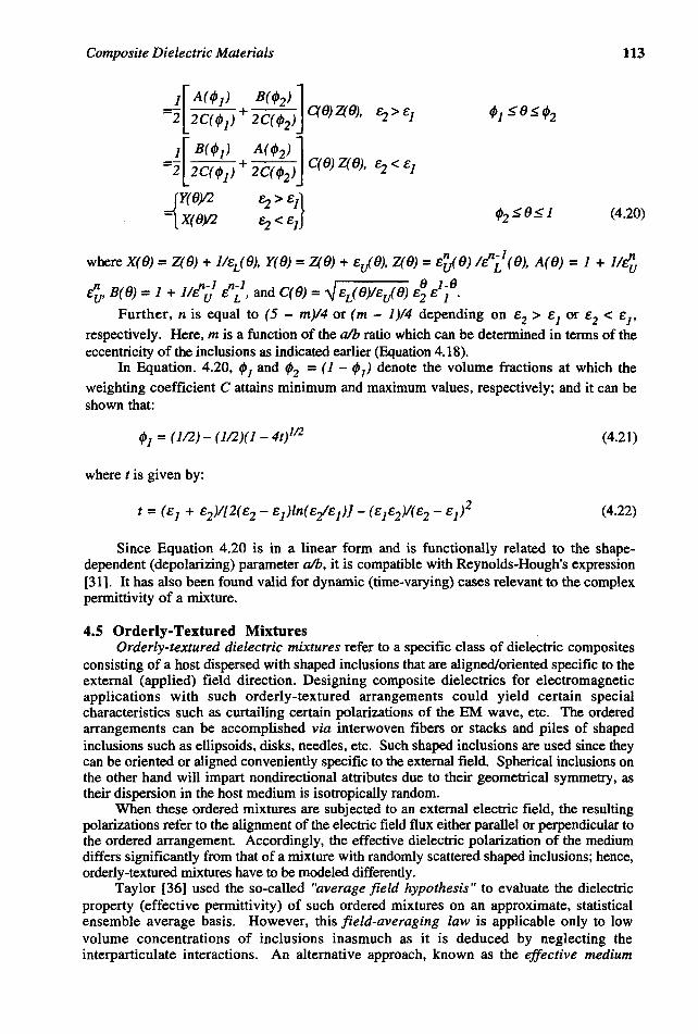
1[A(q,1) B(q,2) ] ="2 2C(q,1) + 2C(q,2) C(8)Z(8),
1[ B(f/>1) A(lP2) ] ="2 2C(f/>1) + 2C(q,2) C(8) Z(8),
={Y(8)12 ~ > e1}
- X(8)12 ~ < e1 (4.20)
where X(8) = Z(8) + 1IeL(8), Y(8) = Z(8) + eJ8), Z(8) = e'lJ8) 11"/ (8), A(8) = 1 + 11e~
E~, B(8) = 1 + 1Ie"i/ e"-/, and C(8) =..J eL(8)IEJ8) e~ ~/. Further, n is equal to (5 - m)/4 or (m - 1)/4 depending on e2> e1 or E2 < E]'
respectively. Here, m is a function of the alb ratio which can be determined in terms of the eccentricity of the inclusions as indicated earlier (Equation 4.18).
In Equation. 4.20, q,1 and q,2 = (1 - q,1) denote the volume fractions at which the weighting coefficient C attains minimum and maximum values, respectively; and it can be shown that:
q,1 = (112) - (112)(1 - 4tl12 (4.21)
where t is given by:
(4.22)
Since Equation 4.20 is in a linear form and is functionally related to the shapedependent (depolarizing) parameter alb, it is compatible with Reynolds-Hough's expression [31]. It has also been found valid for dynamic (time-varying) cases relevant to the complex permittivity of a mixture.
4.5 Orderly-Textured Mixtures Orderly-textured dielectric mixtures refer to a specific class of dielectric composites
consisting of a host dispersed with shaped inclusions that are aligned/oriented specific to the external (applied) field direction. Designing composite dielectrics for electromagnetic applications with such orderly-textured arrangements could yield certain special characteristics such as curtailing certain polarizations of the EM wave, etc. The ordered arrangements can be accomplished via interwoven fibers or stacks and piles of shaped inclusions such as ellipsoids, disks, needles, etc. Such shaped inclusions are used since they can be oriented or aligned conveniently specific to the external field. Spherical inclusions on the other hand will impart nondirectional attributes due to their geometrical symmetry, as their dispersion in the host medium is isotropically random.
When these ordered mixtures are subjected to an external electric field, the resulting polarizations refer to the alignment of the electric field flux either parallel or perpendicular to the ordered arrangement. Accordingly, the effective dielectric polarization of the medium differs significantly from that of a mixture with randomly scattered shaped inclusions; hence, orderly-textured mixtures have to be modeled differently.
Taylor [36] used the so-called "average field hypothesis" to evaluate the dielectric property (effective permittivity) of such ordered mixtures on an approximate, statistical ensemble average basis. However, this field-averaging law is applicable only to low volume concentrations of inclusions inasmuch as it is deduced by neglecting the interparticulate interactions. An alternative approach, known as the effective medium
114 Handbook of Electromagnetic Materials
approximation [37,38] addresses a random mixture whose dielectric property is ascertained by discretizing the medium into independent cells. Again, relevant formulations apply to a small concentration of the inclusions only. The effective medium, in general, replaces the heterogeneous status of the medium by an effective region free of scattering effects [37].
4.5.1 Logarithmic LAw of Mixing and Orderly-Textured Mixtures Consider a simple orderly-textured dielectric mixture constituted by an orderly
arrangement of shaped inclusions in a host medium. The ordered disposition of the inclusions would render the effective dielectric properties (effective permittivity) considerably different from that of a mixture consisting of randomly dispersed shaped inclusions. A weighted exponent strategy described in [35,39] models the orderly-textured test mixture using LAngevin's theory of dipole orientation*· This theory is judiciously applied by the author as described in [40] to extrapolate the disordered particulate state formulation so as to describe a test mixture having an ordered state of inclusions. That is, Langevin's function (which represents the monotonic growth of orientational polarizability with respect to the enhancement of ordered texture) is used as a weighting coefficient in the logarithmic law pertaining to a random system. The dependence of the effective permittivity of an orderlytextured mixture on the shape of the inclusions is thus predicted on the basis of the weighted exponent forms of the logarithmic law.
Therefore, the effective permittivity of a mixture with the prolate/oblate spheroidal inclusions being orderly-textured (parallel or perpendicular to an external field direction) can be specified as follows [40].
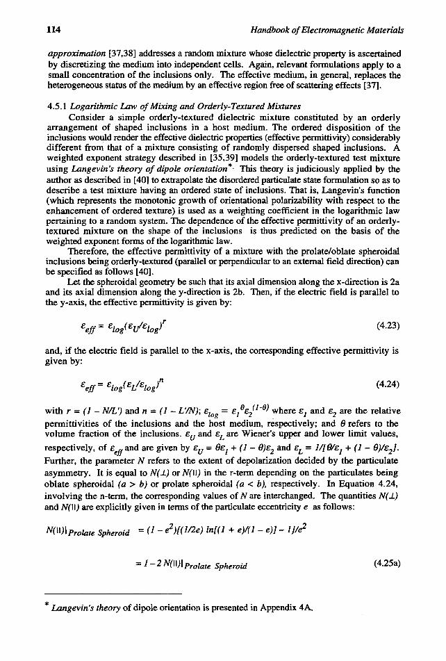
Let the spheroidal geometry be such that its axial dimension along the x-direction is 2a and its axial dimension along the y-direction is 2b. Then, if the electric field is parallel to the y-axis, the effective permittivity is given by:
(4.23)
and, if the electric field is parallel to the x-axis, the corresponding effective permittivity is given by:
(4.24)
with r = (1 - NIL') and n = (J - L'IN); £[(}g = £/£20 -8) where £1 and £2 are the relative permittivities of the inclusions and the host medium, respectively; and 9 refers to the volume fraction of the inclusions. £u and £L are Wiener's upper and lower limit values,
respectively, of £effand are given by £u = 9£1 + (1- 9)£2 and £L = 11[()J£1 + (1- 9)1£2J·
Further, the parameter N refers to the extent of depolarization decided by the particulate asymmetry. It is equal to N(i) or N(II) in the r-term depending on the particulates being oblate spheroidal (a > b) or prolate spheroidal (a < b). respectively. In Equation 4.24, involving the n-term, the corresponding values of N are interchanged. The quantities N( i) and N(II) are explicitly given in terms of the particulate eccentricity e as follows:
N(II)lprolate Spheroid = (1 - ;)((1l2e) In[(l + e)l(l - e)) _l}/e2
= 1 - 2 N(II) I Prolate Spheroid (4.25a)
* Langevin's theory of dipole orientation is presented in Appendix 4A.
Composite Dielectric Materials 115
2)112 1 2 N(II) I Oblate Spheroid ={1-[(l-e l2e)sin- (e)}/e
= 1 - 2 N(II)I Oblate Spheroid (4.25b)
When b »a, the prolate spheroid represents needle-like (fibrous) inclusions and for a» b the oblate spheroid depicts disk-like (flaky) particles.
Further, the parameter L' in Equations 4.23 and 4.24 represents dL(e)/de; when e = 0 or a = b, the particles are spherical and the corresponding slope of L(e) at e = 0, namely, L'(O) = 1/3, which is the well-known order function of the totally disordered state. As e ~ 1, L '( e) ~ 0, representing a totally ordered state corresponding to the particulates being fully aligned with respect to the electric field direction. Hence, Equations 4.23 and 4.24 decide the development of the electrical polarizability (and hence, the permittivity of the mixture) corresponding to the ordered state from the disordered statistics. It does not restrict the amount of particulates present in the mixture. Therefore, it is free from the constraint of dilute-phase approximation.
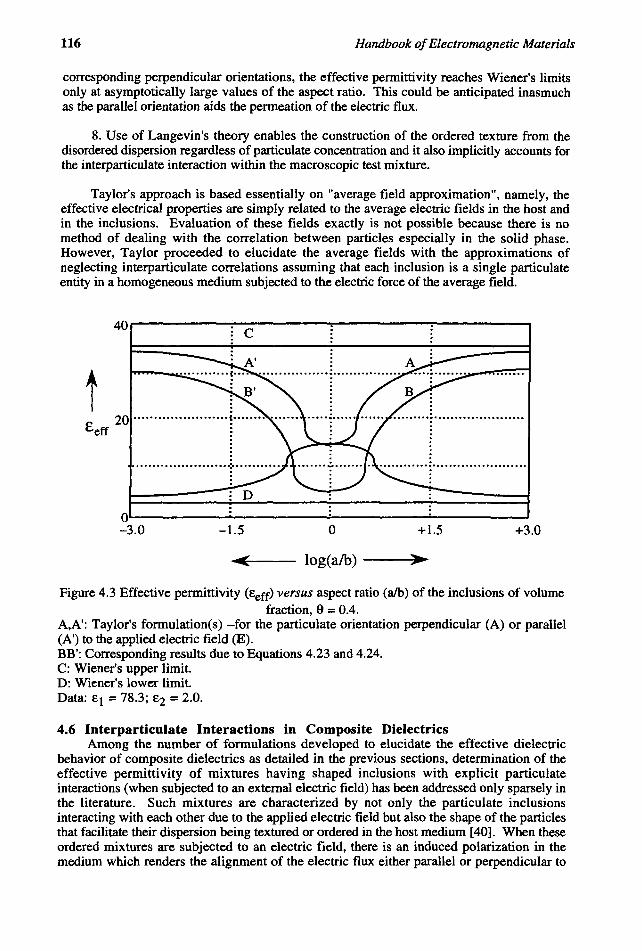
Calculated sample results pertinent to a set of data obtained from Equations 4.23 and 4.24 are depicted in Figure (4.3) wherein the relevant results derived thereof are compared with those due to Taylor [36]. The inferences are:
1. Referring to Figure (4.3), the results due to Taylor's method [36] give a value of Eeff= 14.2 at e = 0, for E] = 78.3, E2 = 2, and a volume fraction of () = 0.4. At e = 0, however, as indicated before, this result should correspond to randomly dispersed spherical/near spherical inclusions with an effective permittivity EefJ = 8.67. Unlike
Taylor's formulation, the method described above gives this value of 8.67 at e = O. The reason for Taylor's result yielding an overestimated value is due to the fact that his results
are based on Bottcher's [10] formula which has the inherent deficiency of short-range statistical variations being neglected.
2. Hence, Taylor's formulations are valid only for high volume concentrations of inclusions (() > 0.4). The formulations of Equations 4.23 and 4.24 are, however, devoid of this deficiency.
3. For large values of e, the present as well as Taylor's formulations are bounded by Wiener's limits. That is, for absolute parallel or perpendicular orientation of the particles with respect to the electric field, both formulations would yield similar results.
4. Except for its values at e = 0 being different, the trends of the variation of £eff with
respect to the aspect ratio as calculated by the present method as well as by Taylor's algorithms remain the same for £] > £2 or £] < £2.
5. For prolate (needle-like) inclusions, the value of the effective permittivity of the mixture tends towards Wiener's upper limit in the limiting case of all the inclusions being aligned parallel to the electric field direction. Likewise, when all the inclusions are antiparallel (perpendicular) to the applied electric field, the value of the effective permittivity of the mixture tends towards Wiener's lower limit.
6. For oblate (disk-like) inclusions the above trends are reversed.
7. When the needle-like inclusions are aligned with the needle-axis parallel to the electric field (or when the electric field is tangential to the surface of the disk-like inclusions), the effective permittivity saturates to Wiener's upper limit (or Wiener's lower limit, respectively) even at relatively low aspect ratios. On the contrary, with the
116 Handbook of Electromagnetic Materials
corresponding perpendicular orientations, the effective permittivity reaches Wiener's limits only at asymptotically large values of the aspect ratio. This could be anticipated inasmuch as the parallel orientation aids the permeation of the electric flux.
8. Use of Langevin's theory enables the construction of the ordered texture from the disordered dispersion regardless of particulate concentration and it also implicitly accounts for the interparticulate interaction within the macroscopic test mixture.
Taylor's approach is based essentially on "average field approximation", namely, the effective electrical properties are simply related to the average electric fields in the host and in the inclusions. Evaluation of these fields exactly is not possible because there is no method of dealing with the correlation between particles especially in the solid phase. However, Taylor proceeded to elucidate the average fields with the approximations of neglecting interparticulate correlations assuming that each inclusion is a single particulate entity in a homogeneous medium subjected to the electric force of the average field.
40r---------~----------~--------~--------~ C
O~----------------------~--------------------~ -3.0 -1.5 o +1.5 +3.0
log(alb) --;~~
Figure 4.3 Effective permittivity (£eff) versus aspect ratio (alb) of the inclusions of volume fraction, () = 0.4.
A,A': Taylor's formulation(s) -for the particulate orientation perpendicular (A) or parallel (A') to the applied electric field (E). BB': Corresponding results due to Equations 4.23 and 4.24. C: Wiener's upper limit. D: Wiener's lower limit. Data: £1 = 78.3; £2 = 2.0.
4.6 Interparticulate Interactions in Composite Dielectrics Among the number of formulations developed to elucidate the effective dielectric
behavior of composite dielectrics as detailed in the previous sections, determination of the effective permittivity of mixtures having shaped inclusions with explicit particulate interactions (when subjected to an external electric field) has been addressed only sparsely in the literature. Such mixtures are characterized by not only the particulate inclusions interacting with each other due to the applied electric field but also the shape of the particles that facilitate their dispersion being textured or ordered in the host medium [40]. When these ordered mixtures are subjected to an electric field, there is an induced polarization in the medium which renders the alignment of the electric flux either parallel or perpendicular to
Composite Dielectric Materials 117
the ordered arrangement. Also, certain classes of electromagnetic "soft materials" constituted by a dispersion of dielectric particles in weakly conducting or dielectric fluids (known popularly as the electrorheological fluids; see Chapter 24) exhibit spontaneous alignment of the particles under the application of an external field. In such cases, the particles may assume dispositions of being nearly in physical contact with each other. This close proximity would result in significant mutual interactions between them which must be duly taken into account in describing the effective dielectric response of the composite material.
The analytical strategy to examine such interaction is to consider a multipolar field expansion in the vicinity of interacting particles and determine the coefficients of expansion for a subsequent use in formulating the effective dielectric response of the mixture. Lam [41] followed this technique using Rayleigh's [5] method for the multipolar field expansion and deduced the expansion coefficients via orthogonalization of the Legendre functions (in the potential expansion) in the case of spherical particles. Thus, in the presence of an external field inducing interparticulate interactions, the theoretical considerations in formulating the effective dielectric response of the mixture consisting of shaped inclusions can be specified by a multipolar electric field potential expansion method. This technique facilitates the calculation of electrostatic interaction forces between dielectric particles as a function of particle separation. It can be postulated that the change in electrostatic interaction force between the particles with respect to varying the relative spatial dispositions of the constituents can be considered as being proportional to a corresponding change in an order parameter u; and the effective permittivity of the mixture can be described by a functional relation which includes this order parameter to specify the implicit effects of particle interactions [42].
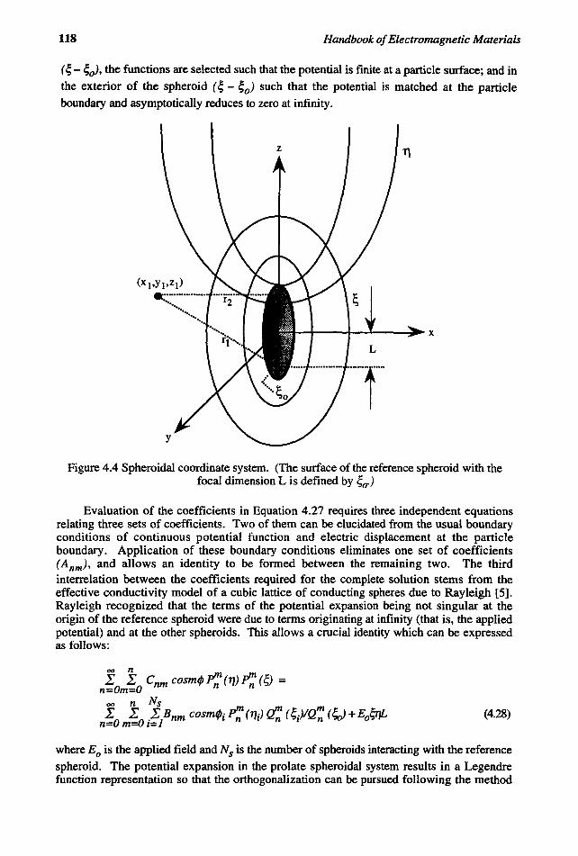
Pertinent to a mixture with spherical particles, the potential function expansion which is valid at all points outside the interacting spheres and includes an arbitrary number of mUltipolar moments can be expressed in terms of spherical harmonics as indicated by Morse and Feshbach [43]. Such a multipolar expansion includes induced contributions arising from the effects of particle proximity, and additional multipole contributions will accrue in the case of shaped particles. To comply with the particulate geometry, the spheroidal coordinate system shown in Figure 4.4 can be considered in describing the potential function.
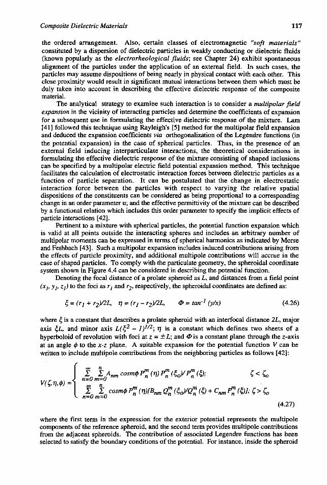
Denoting the focal distance of a prolate spheroid as L, and distances from a field point (Xl' YI' Zl) to the foci as rl and r2' respectively. the spheroidal coordinates are defined as:
tP = tan-J (y/x) (4.26)
where ~ is a constant that describes a prolate spheroid with an interfocal distance 2L, major axis ~L, and minor axis L( ~2 - 1)112; 1] is a constant which defines two sheets of a hyperboloid of revolution with foci at z = ± L; and tP is a constant plane through the z-axis at an angle iP to the x-z plane. A suitable expansion for the potential function V can be written to include multipole contributions from the neighboring particles as follows [42]:
{
n~o m~lnm cosmiP P;: (1]) p; ( ~oJ/ P;: (~); , < '0 V(',1],iP) = co n
n~O m~O cosmiP p; (1])[Bnm f:t:: (~oYQ~ (~) + Cnm P: (~)],. ,> '0 (4.27)
where the first term in the expression for the exterior potential represents the multipole components of the reference spheroid, and the second term provides multipole contributions from the adjacent spheroids. The contribution of associated Legendre functions has been selected to satisfy the boundary conditions of the potential. For instance, inside the spheroid
118 Handbook of Electromagnetic Materials
(; - ;0)' the functions are selected such that the potential is finite at a particle surface; and in
the exterior of the spheroid (; - ;0) such that the potential is matched at the particle
boundary and asymptotically reduces to zero at infinity.
z
--~---+--~--~~x
Figure 4.4 Spheroidal coordinate system. (The surface of the reference spheroid with the focal dimension L is defined by ;0.)
Evaluation of the coefficients in Equation 4.27 requires three independent equations relating three sets of coefficients. Two of them can be elucidated from the usual boundary conditions of continuous potential function and electric displacement at the particle boundary. Application of these boundary conditions eliminates one set of coefficients (Anm), and allows an identity to be formed between the remaining two. The third interrelation between the coefficients required for the complete solution stems from the effective conductivity model of a cubic lattice of conducting spheres due to Rayleigh [5]. Rayleigh recognized that the terms of the potential expansion being not singular at the origin of the reference spheroid were due to terms originating at infinity (that is, the applied potential) and at the other spheroids. This allows a crucial identity which can be expressed as follows:
(4.28)
where Eo is the applied field and Ns is the number of spheroids interacting with the reference
spheroid. The potential expansion in the prolate spheroidal system results in a Legendre function representation so that the orthogonalization can be pursued following the method
Composite Dielectric Materials 119
due to Lam [41]. In order to facilitate the orthogonalization. Equation 4.29 can be transformed into spherical coordinates (r.O) via: r1 = r + L cosO. r2 = r - L cosO and the corresponding prolate spheroidal coordinates are given by ~ = riL. 1] = cosO. Hence. Equation 4.28 can now be expressed as:
(4.29)
where r L = rlL and r 0 refers to the spheroid surface. Application of the orthogonality properties eliminates one of the expansion
coefficients and results in an infinite series solution for the remaining coefficient. By assuming that the position vector with respect to the reference sphere of the calculated field point is of smaller magnitude than the position vector of the ith interacting spheroid, and by neglecting the interactions from the particles not along the line of electric flux (which imposes an azimuthal isotropicity with m = 0 in the foregoing expressions). the expansion coefficient is expressed explicitly by:
where
and
with
[41r1(2n+l)]BnHn = ~~ Dn.n{RLj)Bn, + (41r13)Eo~nl n l
(4.30)
Thus, Equation 4.30 is an infinite series depicting the final boundary condition required to evaluate the coefficients in the potential expansion. The algebraic expansion of Equation 4.30 can be cast in the form of a matrix equation which can be numerically approximated given a finite number of contributing terms N as indicated by the convergence of the series. Once the Bn's are determined, the electric field components are obtained via appropriate spatial differentiation of the potential functions resulting in explicit field components specified by:
(4.31)
at the points exterior to the spheroid.
120 Handbook of Electromagnetic Materials
4.6.1 Electrostatic interaction forces The force experienced by a particle along the (particle) axis parallel to the electric field
is specified as [42]:
Fz = [(E7I£1) -1] fEr -EzdS (4.32) s
which dictates that the interparticle electrostatic force is proportional to the surface integral of the radial and vertical field product. Thus, for a given spatial geometry, the interparticulate force can be considered as being directly proportional to the sum of the product of contributing coefficients in the expansion of the electric field.
This interaction force arising from the external field will influence the dielectric behavior of the mixture. Therefore, to include such interaction effects implicitly in deciding the effective dielectric response of the mixture, an order parameter can be stipulated in terms of the interaction force quantified via Equation (4.32) as a function of the interparticle separation. Hence, an expression to determine the effective permittivity of the mixture involving the order parameter explicitly can be derived as indicated in the following section.
4.6.2 Dielectric mixture model with finite inter particulate interactions When the mixture under consideration is subjected to a uniform electric field, the
particles (either by design, or spontaneously) have a tendency to align to form a chain-like, orderly texture either parallel or perpendicular to the applied field (Figure 4.5). The effective permittivity (Eefi is then determined by the spatial hierarchy of particulate dispersion, the volume fractions of the constituents and the interactive effects among the particles along the lines of electric flux. The mixture formulation to determine the Eeff of aN-component statistical mixture can be represented in a general form as:
(4.33)
where OJ denotes the volume fraction of the ith constituent; and F is a function that implicitly includes the effects of particle orientation, shape, and interactions. The upper and lower bounds, respectively, over the span 0 ~ () ~ 1 are specified by the corresponding functionals Fup and Flo. Within these limits, the bounded value of Eeffcan be derived from the principles of statistical mixture theory, by deducing the homogeneous function F of Equation 4.33 explicitly.
Evaluation of such a functional relation is straightforward in the limiting cases of extreme spatial anisotropy (namely, parallel and series arrangements); however, it is rather difficult to obtain an explicit expression for Eeff for random dispersion of the constituents characterized by the stochastic (spatial) attributes of the Ej • In such cases, an algorithmic approach to describe the effective material response (in terms of the known limiting values) can be written as follows:
(4.34)
where the order parameter u E [0,11, weights the limiting values of the extreme anisotropic spatial arrangements to match the effective material response under a particular spatial configuration and thereby it also implicitly accounts for the particle interactions.
In the case of significant particle eccentricities, or when the mixture constituents tend to form laminar/columnar structures, the bounds F up and Flo as mentioned earlier are
Composite Dielectric Materials 121
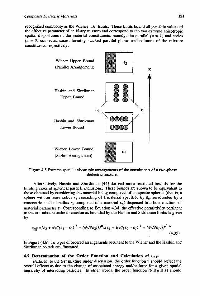
recognized commonly as the Wiener [16] limits. These limits bound all possible values of the effective parameter of an N-ary mixture and correspond to the two extreme anisotropic spatial dispositions of the material constituents, namely, the parallel (u = 1) and series (u = 0) connected cases, forming stacked parallel planes and columns of the mixture constituents, respectively.
Wiener Upper Bound
(Parallel Arrangement)
Rashin and Shtrikman
Upper Bound
Rashin and Shtrikman
Lower Bound
Wiener Lower Bound
(Series Arrangement)
E
[Ill •...• . .....
£2 '. £1
l==Y ••••••••
Figure 4.5 Extreme spatial anisotropic arrangements of the constituents of a two-phase dielectric mixture.
Alternatively, Rashin and Shtrikman [44] derived more restricted bounds for the limiting cases of spherical particle inclusions, These bounds are shown to be equivalent to those obtained by considering the material being composed of composite spheres (that is, a sphere with an inner radius r a consisting of a material specified by Ea, surrounded by a concentric shell of radius rb composed of a material Eb) dispersed in a host medium of material parameter E. Corresponding to Equation 4.34, the effective permittivity pertinent to the test mixture under discussion as bounded by the Rashin and Shtrikman limits is given by:
In Figure (4.6), the types of ordered arrangements pertinent to the Wiener and the Rashin and Shtrikman bounds are illustrated.
4.7 Determination of the Order Function and Calculation of edr Pertinent to the test mixture under discussion, the order function u should reflect the
overall effects as due to the change of associated energy and/or force for a given spatial hierarchy of interacting particles. In other words, the order function (0 ~ u ~ 1) should
122 Handbook of Electromagnetic Materials
correspond to a normalized electrostatic force (0 S FIFo S 1) of interacting particles with respect to particle separation. Here, the normalization of the interaction force is done with respect to a value Fo obtained when the particle separation tends to zero.
The specific algorithmic approach in modeling the effective permittivity of the test mixture can be outlined as follows:
• Determine the mUltipolar electric field potential around a reference particle (Equation 4.31).
• Calculate the electrostatic interaction force of the reference and adjacent particles as a function of varying particle spatial dispositions (Equation 4.32).
• Normalize the interaction force with respect to the limiting value when the particle separation tends to zero.
• Take values of the spatial order parameter u, for a given spatial configuration from the corresponding normalized interaction force.
• Apply the order parameter to the mixture formula (Equations 4.34 and 4.35).
The theoretical considerations presented here to evaluate the effective permittivity of the test mixture refers to both the nonspherical (spheroidal) particulate inclusions with eccentricity (e> 0) and spherical particles with e ~ O. In either case, the relevant analysis includes the effects of interparticulate interactions.
4.8 Sample Results
if ........... ~ ............... .
!
0.1 0.2 0.3 Volume fraction (8)
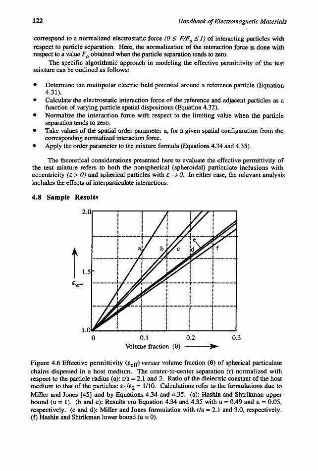
Figure 4.6 Effective permittivity (£eff) versus volume fraction (8) of spherical particulate chains dispersed in a host medium. The center-to-center separation (r) normalized with respect to the particle radius (a): ria = 2.1 and 3. Ratio of the dielectric constant of the host medium to that of the particles: £1/£2 = 1110. Calculations refer to the formulations due to Miller and Jones [45] and by Equations 4.34 and 4.35. (a): Hashin and Shtrikman upper bound (u = 1). (b and e): Results via Equation 4.34 and 4.35 with u = 0.49 and u = 0.05, respectively. (c and d): Miller and Jones formulation with rIa = 2.1 and 3.0, respectively. (f) Hashin and Shtrikman lower bound (u = 0).
Composite Dielectric Materials 123
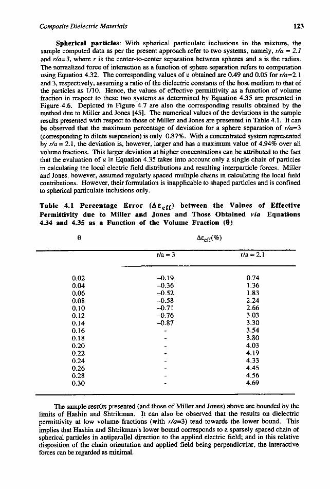
Spherical particles: With spherical particulate inclusions in the mixture, the sample computed data as per the present approach refer to two systems, namely, ria = 2.1 and rla=3, where r is the center-to-center separation between spheres and a is the radius. The normalized force of interaction as a function of sphere separation refers to computation using Equation 4.32. The corresponding values of u obtained are 0.49 and 0.05 for rla=2.1 and 3, respectively, assuming a ratio of the dielectric constants of the host medium to that of the particles as 1110. Hence, the values of effective permittivity as a function of volume fraction in respect to these two systems as determined by Equation 4.35 are presented in Figure 4.6. Depicted in Figure 4.7 are also the corresponding results obtained by the method due to Miller and Jones [45]. The numerical values of the deviations in the sample results presented with respect to those of Miller and Jones are presented in Table 4.1. It can be observed that the maximum percentage of deviation for a sphere separation of rla=3 (corresponding to dilute suspension) is only 0.87%. With a concentrated system represented by ria = 2.1, the deviation is, however, larger and has a maximum value of 4.94% over all volume fractions. This larger deviation at higher concentrations can be attributed to the fact that the evaluation of u in Equation 4.35 takes into account only a single chain of particles in calculating the local electric field distributions and resulting interparticle forces. Miller and Jones, however, assumed regularly spaced mUltiple chains in calculating the local field contributions. However, their formulation is inapplicable to shaped particles and is confined to spherical particulate inclusions only.
Table 4.1 Percentage Error (A£eff) between the Values of Effective Permittivity due to Miller and Jones and Those Obtained via Equations 4.34 and 4.35 as a Function of the Volume Fraction (9)
e
0.02 0.04 0.06 0.08 0.10 0.12 0.14 0.16 0.18 0.20 0.22 0.24 0.26 0.28 0.30
rIa = 3
-0.19 -0.36 -0.52 -0.58 -0.71 -0.76 -0.87
rIa = 2.1
0.74 1.36 1.83 2.24 2.66 3.03 3.30 3.54 3.80 4.03 4.19 4.33 4.45 4.56 4.69
The sample results presented (and those of Miller and Jones) above are bounded by the limits of Hashin and Shtrikman. It can also be observed that the results on dielectric permittivity at low volume fractions (with rla=3) tend towards the lower bound. This implies that Hashin and Shtrikman's lower bound corresponds to a sparsely spaced chain of spherical particles in antiparallel direction to the applied electric field; and in this relative disposition of the chain orientation and applied field being perpendicular, the interactive forces can be regarded as minimal.
124 Handbook of Electromagnetic Materials
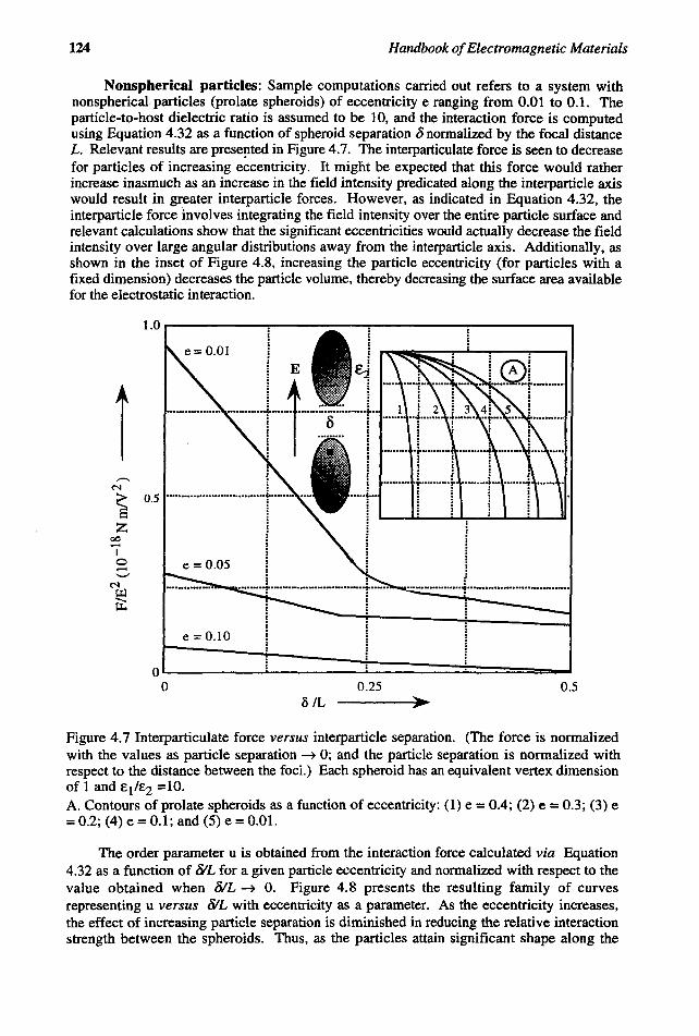
Nonspherical particles: Sample computations carried out refers to a system with nonsphericalparticles (prolate spheroids) of eccentricity e ranging from 0.01 to 0.1. The particle-to-host dielectric ratio is assumed to be 10, and the interaction force is computed using Equation 4.32 as a function of spheroid separation 0 normalized by the focal distance L. Relevant results are prese!1ted in Figure 4.7. The interparticulate force is seen to decrease for particles of increasing eccentricity. It might be expected that this force would rather increase inasmuch as an increase in the field intensity predicated along the interparticle axis would result in greater interparticle forces. However, as indicated in Equation 4.32, the interparticle force involves integrating the field intensity over the entire particle surface and relevant calculations show that the significant eccentricities would actually decrease the field intensity over large angular distributions away from the interparticle axis. Additionally, as shown in the inset of Figure 4.8, increasing the particle eccentricity (for particles with a fixed dimension) decreases the particle volume, thereby decreasing the surface area available for the electrostatic interaction.
1.0~--------~~--------~----------~----------~
I N
~ 0.5 S Z
00
I' 0 -'-'
N
~ JJ..
e = 0.10
0 0 0.25 0.5
B IL > Figure 4.7 Interparticulate force versus interparticle separation. (The force is normalized with the values as particle separation ~ 0; and the particle separation is normalized with respect to the distance between the foci.) Each spheroid has an equivalent vertex dimension of 1 and £1/£2 =10. A. Contours of prolate spheroids as a function of eccentricity: (1) e = 0.4; (2) e = 0.3; (3) e = 0.2; (4) e = 0.1; and (5) e = 0.01.
The order parameter u is obtained from the interaction force calculated via Equation 4.32 as a function of /5/L for a given particle eccentricity and normalized with respect to the value obtained when oIL ~ o. Figure 4.8 presents the resulting family of curves representing u versus /5/L with eccentricity as a parameter. As the eccentricity increases, the effect of increasing particle separation is diminished in reducing the relative interaction strength between the spheroids. Thus, as the particles attain significant shape along the
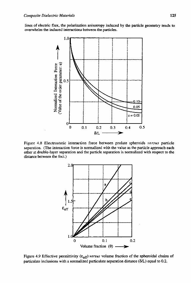
Composite Dielectric Materials 125
lines of electric flux, the polarization anisotropy induced by the particle geometry tends to overwhelm the induced interactions between the particles.
t ~ i ·--r····-r·······r--··r·_···-~ [0.5 ...................... · .... ·1 .. · ............................ · .................... · il ~ i i i] I;
.... ·O.IO'·
0.05
e= 0.01
1 i ····--·-r·-·l··_· o~--~----~----~----~--~ o 0.1 0.2 0.3 0.4 0.5
oIL ----:ilI;>.-
Figure 4.8 Electrostatic interaction force between prolate spheroids versus particle separation. (The interaction force is normalized with the value as the particle approach each other at double-layer separation and the particle separation is normalized with respect to the distance between the foci.)
2.~----~------~----~--~
i 1.5 ~~~~~=~=t= .... Eeff ··· .... ··· .. ·· .. ·1· .......... .
o 0.1 0.2
> Volume fraction (9) ----,:.-
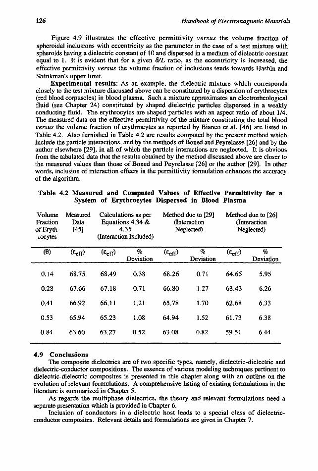
Figure 4.9 Effective permittivity (Eeff) versus volume fraction of the spheroidal chains of particulate inclusions with a normalized particulate separation distance (OIL) equal to 0.2.
126 Handbook of Electromagnetic Materials
Figure 4.9 illustrates the effective permittivity versus the volume fraction of spheroidal inclusions with eccentricity as the parameter in the case of a test mixture with spheroids having a dielectric constant of 10 and dispersed in a medium of dielectric constant equal to 1. It is evident that for a given 8/L ratio, as the eccentricity is increased, the effective permittivity versus the volume fraction of inclusions tends towards Hashin and Shtrikman's upper limit.
Experimental results: As an example, the dielectric mixture which corresponds closely to the test mixture discussed above can be constituted by a dispersion of erythrocytes (red blood corpuscles) in blood plasma. Such a mixture approximates an electrorheological fluid (see Chapter 24) constituted by shaped dielectric particles dispersed in a weakly conducting fluid. The erythrocytes are shaped particles with an aspect ratio of about 114. The measured data on the effective permittivity of the mixture constituting the total blood versus the volume fraction of erythrocytes as reported by Bianco et al. [46] are listed in Table 4.2. Also furnished in Table 4.2 are results computed by the present method which include the particle interactions, and by the methods of Boned and Peyrelasse [26] and by the author elsewhere [29], in all of which the particle interactions are neglected. It is obvious from the tabulated data that the results obtained by the method discussed above are closer to the measured values than those of Boned and Peyrelasse [26] or the author [29). In other words, inclusion of interaction effects in the permittivity formulation enhances the accuracy of the algorithm.
Table 4.2 Measured and Computed Values of Effective Permittivity for a System of Erythrocytes Dispersed in Blood Plasma
Volume Measured Calculations as per Method due to [29] Method due to [26) Fraction Data Equations 4.34 & (Interaction (Interaction of Eryth- [45] 4.35 Neglected) Neglected) rocytes (Interaction Included)
(9) (Eeff) (Eeff) % (Eeff) % (Eeff) % Deviation Deviation Deviation
0.14 68.75 68.49 0.38 68.26 0.71 64.65 5.95
0.28 67.66 67.18 0.71 66.80 1.27 63.43 6.26
0.41 66.92 66.11 1.21 65.78 1.70 62.68 6.33
0.53 65.94 65.23 1.08 64.94 1.52 61.73 6.38
0.84 63.60 63.27 0.52 63.08 0.82 59.51 6.44
4.9 Conclusions The composite dielectrics are of two specific types, namely, dielectric-dielectric and
dielectric-conductor compositions. The essence of various modeling techniques pertinent to dielectric-dielectric composites is presented in this chapter along with an outline on the evolution of relevant formulations. A comprehensive listing of existing formulations in the literature is summarized in Chapter 5.
As regards the multiphase dielectrics, the theory and relevant formulations need a separate presentation which is provided in Chapter 6.
Inclusion of conductors in a dielectric host leads to a special class of dielectricconductor composites. Relevant details and formulations are given in Chapter 7.
Composite Dielectric Materials 127
In addition to the various methods of classifying and modeling dielectric mixtures indicated in this chapter, the other apporaches envisaged in the existing literature are summarized below: Multiscattering models: (i) In a model based on weak fluctuation theory, a mean permittivity value of the mixture has been defined in terms of the permittivities of the host and the inclusions and the volume fractions of the constituents. Then by using a spherical symmetric correlation function for the dielectric permittivity fluctuations, Tsang and Kong [47] have predicted the effective permittivity of the medium in terms of the normalized variance of the fluctuations (..:1) valid for any value of the volume fractions of the inclusions (9j ), if..:1 «1. Otherwise, the corresponding formulation is restricted to 8; «1 (dilute phase approximation of the inclusions). (ii) Another approach advocated by Kong [48] evalutes the complex effective permittivity of the mixture by combining the Maxwell-Garnett formula and that derived by the Rayleigh scattering theory. The corresponding formulation reduces to the quasi static Maxwell-Garnett-Rayleigh equation at low frequencies. (iii) Also, exclusive for spherical scatterers, the effective permittivity has been deduced via effective field approximation [37]. (iv) Using strong fluctuation theory for a random medium, the effective permittivity relevant to a continuous medium has been derived by Tsang et al. [49] assuming a symmetric correlation function. Corresponding results have been shown to
degenerate to Bottcher's formula under low frequency limits [37].
Effective medium approach: This modeling strategy is based on replacing a heterogeneous medium by an effective medium in which the electromagnetic propagation constant is, on an average, assumed to be free from scattering effects. Corresponding quasistatic results on the effective permittivity have been deduced under low frequency limiting conditions. (Relevant formulations have also been extended to composites with conducting inclusions which will be described later in Chapter 6.)
References [1] P. S. Neelakanta: Complex permittivity of chaotic dielectric mixtures: A review. J.
Instr. Electron. Telecom. Engrs; vol. 37(4), 1994: 385-392.
[2] H. Frohlich: Theory of Dielectrics. (Clarendon Press, Oxford: 1949).
[3] J. C. Maxwell-Garnett: Colours in metal glasses and metal films. Phil. Trans. A: Roy. Soc. London. vol. 203, 1904: 385-420.
[4] J. C. Maxwell-Garnett: Colours in metal glasses, in metallic films and in metallic solutions-D. Phil. Trans. A: Roy. Soc. London, vol. 205, 1906: 237-262.
[5] Lord Rayleigh: On the influence of obstacles arranged in rectangular order upon the properties of a medium. Phil. Mag., vol. 34, 1892: 481-502.
[6] D. A. G. Bruggeman: Berechnung verschiedener physikalischer konstantan von heterogenen Substanzen. Ann. Physik, vol. 24, 1935: 636-679.
[7] G. E. Archie: The electrical resistivity log as an aid in determining some reservoir characteristics. Trans. Am. Inst. Min. Met., Petrol. Engrs. vol. 146, 1942: 54-62.
[8] H. Fricke: A mathematical treatment of the electrical conductivity and capacity of disperse systems I. Phys. Review, vol. 24, 1924: 575-587.
[9] H. Fricke: A mathematical treatment of the electrical conductivity and capacity of disperse systems D. Phys. Review, vol. 26, 1926: 687-681.