
CHAPTER 4 - WileyApplication 4.1 lthough economists ascribe an important role to price in...
36
CHAPTER 4 Individual and Market Demand How do individuals’ consumption choices respond to price changes and how is the market demand curve derived from individual consumers’ demand curves?
Transcript of CHAPTER 4 - WileyApplication 4.1 lthough economists ascribe an important role to price in...

CHAPTER 4Individual and Market Demand
How do individuals’ consumption choices respond to price changes andhow is the market demand curve derived from individual consumers’
demand curves?

Chapter Outline
4.1 Price Changes and Consumption ChoicesThe Consumer’s Demand Curve Some Remarks About the Demand CurveApplication 4.1 Using Price to Deter Youth Alcohol Abuse, Traffic Fatalities,and Campus ViolenceApplication 4.2 Sales Tax Avoidance and Online CommerceDo Demand Curves Always Slope Downward?
4.2 Income and Substitution Effects of a Price ChangeIncome and Substitution Effects Illustrated: The Normal-Good CaseApplication 4.3 Income and Substitution Effects and Home OwnershipThe Income and Substitution Effects Associated with a Gasoline-Tax-Plus-Rebate Program
4.3 Income and Substitution Effects: Inferior GoodsThe Giffen Good Case: How Likely?Application 4.4 Do Rats Have Downward-Sloping Demand Curves?
4.4 From Individual to Market DemandApplication 4.5 Aggregating Demand Curves for a UCLA MBA
4.5 Consumer SurplusApplication 4.6 The Consumer Surplus Associated with Free TVConsumer Surplus and Indifference Curves
4.6 Price Elasticity and the Price-Consumption CurveApplication 4.7 The P-C Curve for a non-P-C Good
4.7 Network EffectsThe Bandwagon Effect The Snob EffectApplication 4.8 Network Effects and the Diffusion of CommunicationsTechnologies and Computer Hardware and Software
4.8 The Basics of Demand EstimationExperimentation Surveys Regression AnalysisApplication 4.9 Demand Estimation: McDonald’s Versus Burger King
81
Learning Objectives• Understand how price changes affect consumption choices.• Differentiate between the income and substitution effects associated with a
price change on the consumption of a particular good.• Explain the relation between income and substitution effects in the case of
inferior goods.• Show how individual demand curves are aggregated to obtain the market
demand curve.• Demonstrate how consumer surplus represents the net benefit, or gain, served
by an individual from consuming one market basket instead of another.• Investigate the relationship between own-price elasticity of demand and the
price-consumption curve.• Examine network effects: the extent to which an individual consumer’s
demand for a good is influenced by other individuals’ purchases.• Overview the basics of demand estimation.

82 Chapter Four • Individual and Market Demand •
n Chapter 3, we developed a model using indifference curves and budget lines to ex-plain consumer behavior and used it to examine how changes in income affect con-
sumer choices. In this chapter we use the consumer choice model to analyze the effects ofprice changes and show how a consumer’s demand curve can be derived using the model.We also discuss how individual demand curves are aggregated to obtain the market demandcurve. In addition, we explain the concept of consumer surplus, which relates to how areasunder the demand curve can be used to measure the net benefits or costs to consumers fromchanges in consumption. And finally, we cover demand estimation to show how individuals’or market demand curves can be estimated from real-world data.
This chapter completes our discussion of the basic elements of the theory of consumerchoice. Chapter 5, however, will illustrate the wide range of applications of this theory tosuch diverse problems as pricing garbage collection, deciding how much to save and borrow,and determining how much to invest in various financial assets.
4.1 Price Changes and Consumption Choices1
Let’s examine the way a change in a good’s price affects the market basket chosen by a con-sumer. Because we wish to isolate the effect of a price change on consumption, we holdconstant other factors such as income, preferences, and the prices of other goods.
Figure 4.1a depicts a consumer deciding how to allocate a given amount of annual in-come between college education (C) and all other goods. The per-credit-hour price of col-lege education, $250, is indicated by the slope of the budget line since the per-dollar price ofoutlays on all other goods can be taken to be unity. With an initial budget line of AZ, theconsumer’s optimal consumption point is W. The consumption of college education is C1,and outlays on other goods are A1.
If the price of college education falls from $250 to $200, the budget line rotates aroundpoint A and becomes flatter. With a price of $200, the budget line becomes AZ�, where Z�equals the consumer’s constant income divided by the lower price of college education.Confronted with this new budget line, the consumer selects the most preferred market bas-ket from among those available on AZ�. For the particular preferences shown, the preferredbasket is point W�, where the slope of U2 (the marginal rate of substitution) equals the slopeof the flatter budget line AZ�. Consumption of college education has increased to C2 in re-sponse to the reduction in its price. If the price of college education falls still further to$150, then the budget line becomes AZ�, and the consumer will choose point W�, with theamount of credit hours of college education consumed equal to C3.
Proceeding in this way, we can vary the price of college education and observe the mar-ket basket chosen by the consumer. For every possible price, a different budget line resultsand the consumer selects the market basket that permits attainment of the highest possibleindifference curve. Points W, W�, and W� represent three market baskets associated withprices of $250, $200, and $150, respectively. If we connect these optimal consumptionpoints, and those associated with other prices (not drawn in explicitly), we obtain theprice-consumption curve, shown as the P-C curve in the diagram. The price-consumptioncurve identifies the optimal market basket associated with each possible price of college edu-cation, holding constant all other determinants of demand.
I
1A mathematical treatment of some of the material in this section is given in the appendix at the back of the book(page xxx).
price-consump-tion curvea curve that identifies theoptimal market basketassociated with eachpossible price of a good,holding constant all otherdeterminants of demand

• Price Changes and Consumption Choices 83
The Consumer’s Demand CurveUsing the procedure just described, we can determine the consumer’s demand curve for col-lege education. The demand curve relates consumption of college education to its price,holding constant such factors as income, the prices of related goods, and preferences. Theprice-consumption curve does the same thing although it is not itself the demand curve. Toconvert the price-consumption curve to a demand curve, we simply plot the price-quantityrelationship identified by the price-consumption curve in the appropriate graph.
Figure 4.1b shows the consumer’s demand curve d (as before, we use lowercase letters to in-dicate the individual consumer’s demand curve); it indicates the quantity of college educationthe consumer will buy at alternative prices, other factors held constant. The demand curve is
(a)
(b)
0 C1 Z′ Z′′
U3
U2U1
W′
W
W′′
A1
A2
C2
$250 $200 $150
C3
1C1C
Units of college education
Units of college education
0 C1
F
G
H
d
$250 = P1
$200 = P2
$150 = P3
Per unitprice ofcollegeeducation
C2 C3
Z
A
Othergoods
1C
P-C curve
Figure 4.1Figure 4.1
Derivation of the Consumer’s Demand CurveA reduction in the price of collegeeducation, with income, preferences, andthe prices of other goods remaining fixed,leads the consumer to purchase more units of college education. (a) The optimalmarket baskets associated with alternativeprices for college education are connectedto form the price-consumption curve. (b) The same information is plotted as the consumer’s demand curve for collegeeducation.

Application 4.1
lthough economists ascribe an important role toprice in determining the quantity demanded of a
product, policymakers often do not. A case in point is thecampaign waged by policymakers since the mid-1970s to
A discourage alcohol abuse and thereby decrease the numberof traffic-related deaths. One of the main campaign objec-tives has been to raise the legal age for alcohol consump-tion to 21 years. The reason behind this is that while
84 Chapter Four • Individual and Market Demand •
determined by plotting the price-quantity combinations identified by the price-consumptioncurve in Figure 4.1a. For example, when the price of college education is $250 (the slope ofAZ), consumption of college education is C1 at point W in Figure 4.1a. Figure 4.1b shows theprice of college education explicitly on the vertical axis. When the price is $250, consumptionis C1, so point F locates one point on the demand curve. When the price is $200 (the slope ofAZ�), consumption is C2, which identifies a second point, G, on the demand curve. Otherpoints are obtained in the same manner to plot the entire demand curve d.
Some Remarks About the Demand CurveWe have just derived a consumer’s demand curve from the individual’s underlying prefer-ences (with a given income and fixed prices of other goods). This approach clarifies severalpoints about the demand curve:
1. The consumer’s level of well-being varies along the demand curve. This point is clearfrom Figure 4.1a, where the consumer reaches a higher indifference curve when the price ofcollege education falls. The diagram specifies why the consumer benefits from a lower price:the consumer can now purchase market baskets that were previously unattainable.2. The prices of other goods are held constant along a demand curve, but the quantitiespurchased of these other goods can vary. For example, in Figure 4.1a, consumption of allother goods falls from A1 to A2 when the price of college education falls from $250 to $200.Because all other goods are lumped together and treated as a composite good, the way inwhich consumption of any other specific good may change is not shown explicitly.3. At each point on the demand curve, the consumer’s optimality condition MRSCO �PC/PO is satisfied. (The subscript O refers to other goods, the composite good measured onthe vertical axis.) As the price of college education falls, the value of PC/PO becomessmaller, and the consumer chooses a market basket for which MRSCO, the slope of theindifference curve, is also smaller.4. The demand curve identifies the marginal benefit associated with various levels ofconsumption. The height of the demand curve from the horizontal axis, at each level ofconsumption, indicates the marginal benefit of the good. For example, when consumption is C2
at point G on the demand curve (Figure 4.1b), the distance GC2 (or $200) is a measure of howmuch the marginal unit of college education consumed is worth to the consumer. Why? Refer toFigure 4.1a; for a market basket selected by a consumer to be optimal, such as W� when the priceof college education is $200, MRSCO equals PC/PO. Since PO can be taken to equal unity, thisimplies that MRSCO � PC. Thus, at point W� in Figure 4.1a, MRSCO is equal to $200 per unit ofcollege education. Because the MRS is a measure of what the consumer is willing to give up foran additional credit hour of college education, it is a measure of the marginal benefit. Note that atevery point on the demand curve the height of the demand curve equals the MRS, thereby indicating themarginal benefit of the good to the consumer. For this reason economists refer to the price at whichpeople purchase a given good as revealing the relative importance of the good to them.
Application 4.1 Using Price to Deter Youth Alcohol Abuse, Traffic Fatalities,and Campus Violence

• Price Changes and Consumption Choices 85
3“How to Calm the Campus‚” Business Week‚ November 1‚ 1999‚ p. 32.
people under the age of 25 represent 20 percent of all li-censed drivers, they account for 35 percent of all drivers in-volved in fatal accidents. Alcohol is involved in more thanhalf the driving fatalities accounted for by young drivers.
By raising the legal age for alcohol consumption to 21,policymakers hope to shift the demand curve for alcoholto the left (diminishing the portion of the population withaccess to alcohol) and thereby reduce both alcohol abuseand driving fatalities.
Shifting the demand curve for alcohol to the left isone way to reduce alcohol abuse and traffic fatalities.However, economic research suggests that a more effec-tive method, even among teenagers, would be to raisethe price of alcohol through higher taxes, thereby pro-ducing a movement along the demand curve for alcohol.
The federal tax on alcohol was constant in nominaldollar terms between 1951 and 1991 ($9 per barrel ofbeer, $10.50 per proof gallon of distilled spirits such asvodka, and so on) and has only been increased modestlysince then. In real terms, consequently, the federal taxon alcohol has decreased since 1951. For examples, thereal federal tax on beer has declined by 70 percent since1951 while the real tax on distilled spirits has decreasedby 81 percent. The decline, in real terms, of the federaltax on alcohol is a major factor behind the substantialdecrease in the real price of alcohol since 1951—40 per-cent in the case of beer and 70 percent for hard liquor.
A national survey of teenagers finds that, holdingconstant other factors such as a state’s minimum drink-ing age, religious affiliation, and proximity to borderingstates with lower minimum drinking ages, the amount ofalcohol consumed by the average teenager in a state issignificantly influenced by the price of alcohol there.2
2According to Douglas Coate and Michael Grossman, “Effects of Al-coholic Beverage Prices and Legal Drinking Ages on Youth AlcoholUse,” Journal of Law and Economics, 31 No. 1 (April 1988), pp.145–172, the estimated price elasticity of demand for teenage drinkingranges from 0.5 to 1.2.
The survey findings suggest that raising taxes on al-cohol offers a potent mechanism for deterring alcoholabuse and traffic fatalities among teenagers. Specifi-cally, based on the survey’s results, had federal taxeson alcohol remained constant since 1951 in real pur-chasing power terms rather than in dollar terms,teenage drinking would have fallen more than if theminimum drinking age had been raised to 21 in allstates. Raising the price of drinking and moving alongthe demand curve for alcohol thus promises to bemore effective at reducing teenage drinking than thepolicy pursued by most policymakers—shifting thedemand curve for alcohol to the left by imposing agerestrictions.
According to another study‚ the decline in the realprice of alcohol also appears to have resulted in an in-crease in campus violence over the last decade.3 Cur-rently‚ a third of the college student population of 14.5million in the United States is expected to be in-volved‚ in any given year‚ in same kind of campus vio-lence (arguments‚ fights‚ run-ins with police or collegeauthorities‚ sexual misconduct‚ and so on). Because al-coholic consumption is positively correlated with vio-lence‚ the study examined the relationship betweenprices of six-packs of beer and levels of violence at col-leges around the country. The study found that a 10percent increase in the price of beer would be sufficientto decrease campus violence by 4 percent, other factorsheld constant. However‚ since the real price of beerhas actually fallen by 10 percent since 1991—largelydue to the decline‚ in real items‚ of the federal tax onalcohol—the converse result has occurred. Namely‚the study concludes that campus violence has in-creased by 4 percent (200‚000 incidents) since 1991 onaccount of the decline in the real price of beer.
Application 4.2
n important factor driving online commerce ap-pears to be the fact that local sales taxes generally
are not applied to purchases made on the Internet.
A Using data on the buying decisions of 25‚000 onlineusers‚ Austan Goolsbee of the University of Chicagofinds that‚ holding all other factors constant‚ individuals
Application 4.2 Sales Tax Avoidance and Online Commerce
86 Chapter Four • Individual and Market Demand •
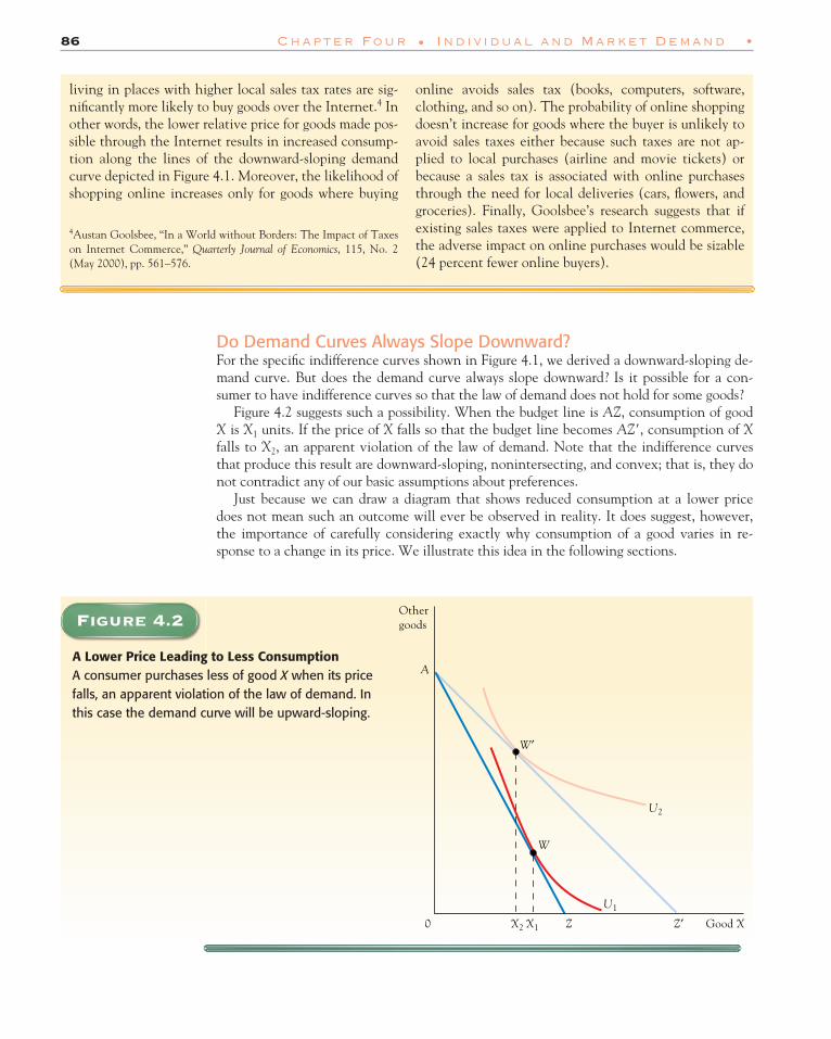
Do Demand Curves Always Slope Downward?For the specific indifference curves shown in Figure 4.1, we derived a downward-sloping de-mand curve. But does the demand curve always slope downward? Is it possible for a con-sumer to have indifference curves so that the law of demand does not hold for some goods?
Figure 4.2 suggests such a possibility. When the budget line is AZ, consumption of goodX is X1 units. If the price of X falls so that the budget line becomes AZ�, consumption of Xfalls to X2, an apparent violation of the law of demand. Note that the indifference curvesthat produce this result are downward-sloping, nonintersecting, and convex; that is, they donot contradict any of our basic assumptions about preferences.
Just because we can draw a diagram that shows reduced consumption at a lower pricedoes not mean such an outcome will ever be observed in reality. It does suggest, however,the importance of carefully considering exactly why consumption of a good varies in re-sponse to a change in its price. We illustrate this idea in the following sections.
0
U1
U2
Othergoods
Good XZ Z′
W′
W
X2 X1
A
Figure 4.2Figure 4.2
A Lower Price Leading to Less ConsumptionA consumer purchases less of good X when its pricefalls, an apparent violation of the law of demand. Inthis case the demand curve will be upward-sloping.
4Austan Goolsbee‚ “In a World without Borders: The Impact of Taxeson Internet Commerce‚” Quarterly Journal of Economics‚ 115‚ No. 2(May 2000)‚ pp. 561–576.
online avoids sales tax (books‚ computers‚ software‚clothing‚ and so on). The probability of online shoppingdoesn’t increase for goods where the buyer is unlikely toavoid sales taxes either because such taxes are not ap-plied to local purchases (airline and movie tickets) orbecause a sales tax is associated with online purchasesthrough the need for local deliveries (cars‚ flowers‚ andgroceries). Finally‚ Goolsbee’s research suggests that ifexisting sales taxes were applied to Internet commerce‚the adverse impact on online purchases would be sizable(24 percent fewer online buyers).
living in places with higher local sales tax rates are sig-nificantly more likely to buy goods over the Internet.4 Inother words‚ the lower relative price for goods made pos-sible through the Internet results in increased consump-tion along the lines of the downward-sloping demandcurve depicted in Figure 4.1. Moreover‚ the likelihood ofshopping online increases only for goods where buying

• Income and Substitution Effects of a Price Change 87
4.2 Income and Substitution Effects of a Price Change
When the price of a good changes, the change affects consumption in two different ways.Normally, we cannot observe these two effects separately. Instead, when the consumer altersconsumption in response to a price change, all we see is the combined effect of both factors.Nevertheless, it is useful to analytically break down the effects of a price change into thesetwo components.
The first way a price change affects consumption is the income effect. When the price ofa good falls, a consumer’s real purchasing power increases, which affects consumption of thegood. A price reduction increases real income—that is, makes it possible for the consumer toattain a higher indifference curve.
The second way a price reduction affects consumption is the substitution effect. Whenthe price of one good falls, the consumer has an incentive to increase consumption of thatgood at the expense of other, now relatively more expensive, goods. The individual’s con-sumption pattern will change in favor of the now less costly good and away from othergoods. In short, the consumer will substitute the less expensive good for other goods—hencethe name substitution effect.
To see intuitively that two different factors are at work when a price changes, compareFigure 3.14 from Chapter 3 and Figure 4.1. In Figure 4.1, a price reduction results in theconsumer reaching a higher indifference curve. In Figure 3.14, an increase in income, withno change in prices, also results in consumers reaching a higher indifference curve. Appar-ently, a common factor is at work: both a reduction in price and an increase in income raisethe consumer’s real income, in the sense of permitting attainment of greater well-being. Inboth cases the budget line moves outward, allowing consumption of market baskets thatwere not previously attainable. This points to one of the two ways a price reduction affectsconsumption: it augments real income (by increasing the purchasing power of a given nomi-nal income), which obviously affects consumption. This is the income effect.
Although a price reduction and an income increase both have an income effect on con-sumption, there is a significant difference between them. With a price reduction the con-sumer moves to a point on a higher indifference curve where the slope is lower than it wasat the original optimal consumption point (see Figure 4.1). In effect, the consumer hasmoved down the indifference curve to consume more of the lower-priced good. This resultillustrates the substitution in favor of the less costly good. When income increases, however,the consumer moves to a point on a higher indifference curve where the slope (the MRS) is the same as it was prior to the income increase. This is so because if only income changes,the slope of the consumer’s budget line does not change. The precise distinction betweenthese two effects and the way they help us understand why the demand curve has the shapeit does are clarified next with a graphical treatment.
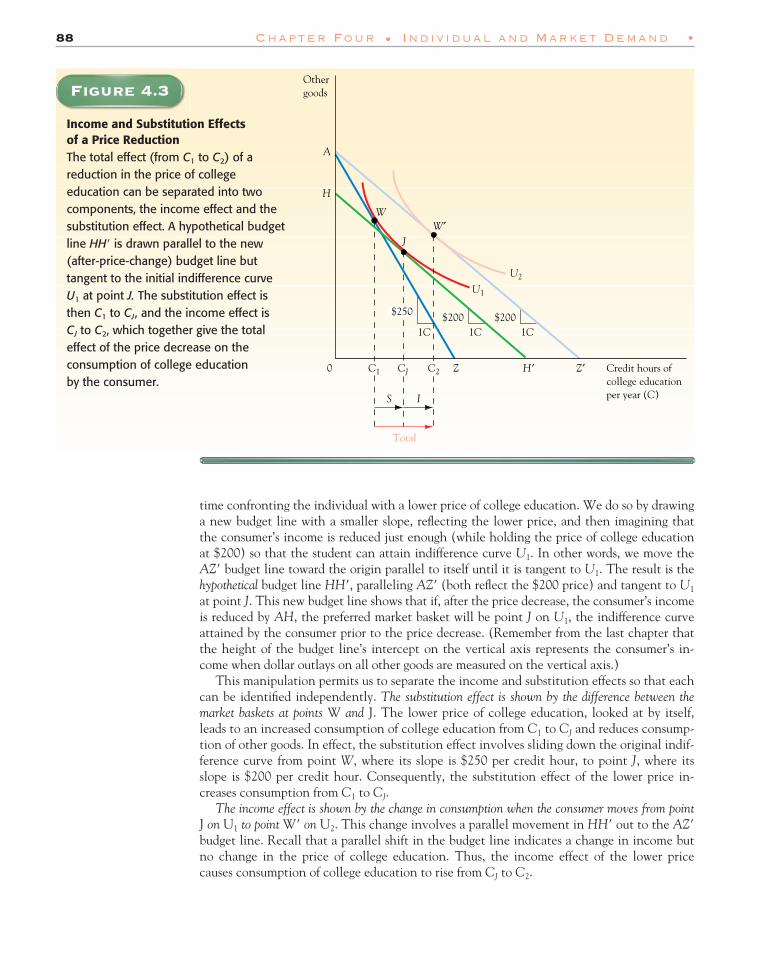
Income and Substitution Effects Illustrated: The Normal-Good CaseIn Figure 4.3, the consumer’s original budget line AZ relates annual credit hours of collegeeducation and outlays on all other goods. At a per-credit-hour price of $250, the optimalmarket basket is W, with C1 credit hours bought by the consumer. If the price of college ed-ucation falls to $200, the budget line becomes AZ�, and the consumer buys C2 units. The in-crease in consumption of college education (from C1 to C2) in response to the lower price isthe total effect of the price reduction on purchases of college education. The demand curveshows the total effect. Now we wish to show how this total effect can be decomposed con-ceptually into its two component parts—the income effect and the substitution effect.
The substitution effect illustrates how the change in relative prices alone affects consump-tion, independent of any change in real income or well-being. To isolate the substitution ef-fect, we must keep the consumer on the original indifference curve, U1, while at the same
income effecta change in a consumer’sreal purchasing powerbrought about by a changein the price of a good
substitutioneffectan incentive to increaseconsumption of a goodwhose price falls, at theexpense of other, nowrelatively more expensive,goods
88 Chapter Four • Individual and Market Demand •
time confronting the individual with a lower price of college education. We do so by drawinga new budget line with a smaller slope, reflecting the lower price, and then imagining thatthe consumer’s income is reduced just enough (while holding the price of college educationat $200) so that the student can attain indifference curve U1. In other words, we move theAZ� budget line toward the origin parallel to itself until it is tangent to U1. The result is thehypothetical budget line HH�, paralleling AZ� (both reflect the $200 price) and tangent to U1
at point J. This new budget line shows that if, after the price decrease, the consumer’s incomeis reduced by AH, the preferred market basket will be point J on U1, the indifference curveattained by the consumer prior to the price decrease. (Remember from the last chapter thatthe height of the budget line’s intercept on the vertical axis represents the consumer’s in-come when dollar outlays on all other goods are measured on the vertical axis.)
This manipulation permits us to separate the income and substitution effects so that eachcan be identified independently. The substitution effect is shown by the difference between themarket baskets at points W and J. The lower price of college education, looked at by itself,leads to an increased consumption of college education from C1 to CJ and reduces consump-tion of other goods. In effect, the substitution effect involves sliding down the original indif-ference curve from point W, where its slope is $250 per credit hour, to point J, where itsslope is $200 per credit hour. Consequently, the substitution effect of the lower price in-creases consumption from C1 to CJ.
The income effect is shown by the change in consumption when the consumer moves from pointJ on U1 to point W� on U2. This change involves a parallel movement in HH� out to the AZ�budget line. Recall that a parallel shift in the budget line indicates a change in income butno change in the price of college education. Thus, the income effect of the lower pricecauses consumption of college education to rise from CJ to C2.
0
U1
J
WW′
U2
Othergoods
Total
S I
1C 1C$200
1C$200
A
H
Credit hours ofcollege educationper year (C)
Z Z′H′C1 C2CJ
$250
Figure 4.3Figure 4.3
Income and Substitution Effects of a Price ReductionThe total effect (from C1 to C2) of areduction in the price of collegeeducation can be separated into twocomponents, the income effect and thesubstitution effect. A hypothetical budgetline HH� is drawn parallel to the new(after-price-change) budget line buttangent to the initial indifference curveU1 at point J. The substitution effect isthen C1 to CJ, and the income effect is CJ to C2, which together give the totaleffect of the price decrease on theconsumption of college education by the consumer.

Application 4.3
he likelihood of home ownership in the UnitedStates increases with income.6 For example‚ 35
percent of families with an annual income of less than$10‚000 own a home versus 68 percent of families withan annual income of between $25‚000 and $49‚999 and93 percent of families with an annual income of$100‚000 or more. This phenomenon is due partly to an
T
6Jeffrey M. Perloff, Microeconomics, 2nd ed. (Boston: Addison-WesleyLongman, 2001) and U.S. Census Bureau, Statistical Abstract of theUnited States: 2001 (Washington, DC: U.S. Government Printing Of-fice, 2001).
• Income and Substitution Effects of a Price Change 89
The sum of the substitution effect (C1 to CJ) and the income effect (CJ to C2) measuresthe total effect (C1 to C2) of the lower price on the consumption of college education. Anychange in price can be separated into income and substitution effects in this manner.
Although this analysis may seem esoteric, it is highly significant. Ultimately, we are seek-ing a firm basis for believing that people will consume more at lower prices—that is, that thelaw of demand is valid. Separating the income and substitution effects allows us to look atthe issue more deeply.
Note that the substitution effect of any price change always implies more consumption of a goodat a lower price and less consumption at a higher price. This relationship follows directly fromthe convexity of indifference curves: with convex indifference curves, a lower price impliesa substitution effect that involves sliding down the initial indifference curve to a pointwhere consumption of the good is greater. Thus, the substitution effect conforms to the lawof demand.
The income effect of a price change, however, implies greater consumption at a lowerprice only if the good is a normal good. In Figure 4.3, when the budget line shifts from HH�to AZ� (a parallel shift), consumption of college education will rise if college education is anormal good.
The demand curve for a normal good must therefore be downward-sloping. Both the substi-tution and income effect of a price change involve greater consumption of the good whenits price is lower.5 Because the total effect is the sum of the income and substitution ef-fects, people will consume more of a normal good when its price is lower. This conclusionis a powerful one, because we know that most goods are normal goods. Some goods are in-ferior goods, however. In Section 4.3 we will explore whether the law of demand appliesto them.
Application 4.3 Income and Substitution Effectsand Home Ownership
5Figure 4.3 shows the substitution and income effects for a price reduction. An increase is handled in a slightly dif-ferent way. If we were considering an increase in the price of college education from $200 to $250 in the diagram,we would accomplish the separation into substitution and income effects by drawing a hypothetical budget linewith a slope of $250 (the new price) tangent to the indifference curve, U2, the consumer is on before the priceincrease.
income effect: home ownership is a normal good‚ and asincome increases‚ so does the likelihood of home owner-ship. A substitution effect‚ however‚ is also at work. Thisis because mortgage interest payments on a home can bededucted from the personal income subject to federaltaxation‚ and the tax rate increases with income. Sincehigher-income individuals can disproportionately re-duce the amount they owe in taxes through the mort-gage interest deduction‚ the relative price of homeownership is lower for them. The lower relative price‚ asubstitution effect‚ thus also encourages a positive corre-lation between income and home ownership.
90 Chapter Four • Individual and Market Demand •
The Income and Substitution Effects Associated with a Gasoline-Tax-Plus-Rebate ProgramEver since the Arab oil embargo in 1973 and the quadrupling of oil prices that resulted fromit, there have been numerous proposals designed to encourage or force U.S. consumers tocut back on their use of gasoline. One such proposal involves the use of a large excise tax ongasoline (roughly 50 cents per gallon) to raise its price and thereby reduce consumption. Anexcise tax is a tax on a specific good such as gasoline that allows the consumer to purchaseas many units of the good at the taxed price as desired.
Realizing that a large gasoline excise tax would place a heavy burden on many families,most proponents of the proposal recommend that the tax revenues be returned to consumersin the form of unrestricted cash transfers, or tax rebates. Alternatively, the tax revenuescould be used to reduce the federal government’s outstanding debt.
Although a sizable increase in gasoline taxes has not yet been enacted into law, it posesan interesting problem. One objection commonly raised to this plan questions whether itwould really cause gasoline consumption to fall. If the revenues from the tax are simply dis-tributed to the general public, why would gas consumption be curtailed? We can use con-sumer choice theory to show that gasoline consumption will, in fact, be reduced by acombination of an excise tax and a tax rebate.
The key to analyzing this policy package is realizing that the tax rebate would be a cashtransfer to each family completely unrelated to its gasoline consumption. In other words, theproposal would not give a rebate of 50 cents for every gallon of gasoline purchased by a fam-ily, because that policy would leave the effective price of gasoline unchanged and com-pletely negate the effect of the tax. Instead, a family would receive a check for $500 a year,for example, regardless of how much gasoline it purchased. On average for all families, therebate would equal the total tax paid, but some families would be overcompensated for thetax while others would be undercompensated.
Now let’s examine the gasoline tax and rebate plan for a representative consumer. Figure4.4a focuses on the effects of such a plan on the representative consumer’s budget line AZ.The excise tax by itself will increase the price from $1.00 to $1.50 per gallon and thereforerotate the budget line inward to AZ�. This is not the end of the analysis, however, becausethe budget line to which the consumer will adjust must reflect both the tax and the rebate.The rebate is shown as the outward parallel shift in AZ� to A�Z�, similar to an increase in in-come, while the price of gasoline remains constant at $1.50 per gallon.
Figure 4.4b depicts what happens to the consumer’s optimal consumption point underthe tax and rebate plan. Initially, the consumer selects point E, along the original budgetline AZ, with G1 gallons being purchased. With the gasoline tax and rebate the consumerselects point E�, where U1 is tangent to the new budget line A�Z�. Gasoline consumptionhas fallen from G1 to G2, while consumption of other goods has increased.
How far out will the tax rebate shift the after-tax budget line, AZ�? If everyone receives arebate of the same size, and it is determined by dividing total tax revenue by the number ofconsumers, then the average consumer will receive a rebate equal to the tax he or she pays.Thus, it seems reasonable to focus the analysis on a consumer who receives a rebate equal tothe tax paid, the situation shown in Figure 4.4b.
To see that the tax and rebate are equal when the consumer’s optimal choice is point E�,note that G2 units of gasoline will be purchased at that point. Because the AZ� budget lineshows the effect of the tax by itself, the total tax revenue is the vertical distance, E�T, be-tween the original budget line, AZ, and the budget line, AZ�, incorporating the tax. We cansee that E�T is the total tax bill by noting that if G2 gallons were purchased when the mar-ket price was $1.00, outlays on other goods would have been vertical distance, E�G2. Oncethe tax is levied, only TG2 in income is left (before the rebate). The vertical difference,E�T, is thus the total tax. Because the rebate equals the tax, the budget line must shift up by
excise taxa tax on a specific good

• Income and Substitution Effects of a Price Change 91
A
$1.50
$1.001G 1G
U2
U1
ET
E′
Othergoods
A
0
(b)
G2 G1 Z ′′ ZZ ′ Gasoline
A′
Othergoods
A
0
(a)
Z ′′ ZZ ′
$1.50 $1.50 $1.00
1G 1G1G
Gasoline
A′
$1.50
1G
Figure 4.5Figure 4.4
Tax-Plus-Rebate ProgramAn excise tax will reduce gasolineconsumption even if the revenue is returnedto taxpayers as lump-sum transfers. (a) Thetax pivots the budget line to AZ� and the taxrebate shifts it to A�Z�. (b) The combinedeffect reduces gasoline consumption from G1 to G2.

92 Chapter Four • Individual and Market Demand •
an amount equal to E�T, and so it passes through point E�. Finally, we have already seenthat point E� represents the consumer’s optimal choice under the tax and rebate plan be-cause the indifference curve is tangent to the final budget line at that point. By experimen-tation, you can determine that if the rebate were any larger, it would be greater than theamount of tax paid and, conversely, less than the tax paid if it were smaller.
The geometry of this case is slightly complicated, but the final outcome fits with commonsense. The excise tax by itself (without a rebate) has an income effect and a substitution ef-fect. Both effects reduce gas consumption—provided, of course, that gas is a normal good inthe case of the income effect. The rebate thus offsets most of the income effect of the tax(but not quite all of it, because the consumer does not return all the way to the original in-difference curve). Thus, the substitution effect determines the final result. Because a higherprice leads the consumer to substitute away from gasoline, the final outcome is reduced gaso-line consumption (G2 versus G1).
Finally, note that this combination of tax and rebate necessarily harms the consumer.This result is true, at least, for any consumer who receives a rebate exactly equal to the tax,because the final outcome will be a market basket on the original budget line inferior to theone selected in the absence of the tax and rebate. Why does anyone propose a policy thatwill make the average family worse off? A good question. Perhaps some consequences arenot fully reflected in this analysis. For example, decreased gasoline purchases mean de-creased Middle Eastern oil imports, and possibly decreased dependence on imported oil isbeneficial in and of itself. In addition, reduced gasoline consumption means lower automo-bile emissions and possibly improved air quality. These benefits are not incorporated intothe analysis, and if they were it is possible that consumers would be better off on balance.
4.3 Income and Substitution Effects: Inferior Goods
Mechanically, the separation of income and substitution effects for a change in the price of aninferior good is accomplished in the same way as for a normal good. The results, however, dif-fer in one significant respect. With a price reduction, the substitution effect still encouragesgreater consumption, but the income effect works in the opposite direction. At a lower pricethe consumer’s real income increases, and this by itself, implies less consumption of an inferiorgood. Thus, a price reduction for an inferior good involves a substitution effect that encouragesmore consumption but an opposing income effect that encourages less consumption. Appar-ently, the total effect—the sum of the income and substitution effects—could go either way.
Figure 4.5a shows one possibility. Initially, the budget line is AZ, with the price of ham-burger at $2 per pound and H1 pounds purchased. When the price falls to $1 per pound, thebudget line pivots out to AZ�, and hamburger consumption rises to H2 pounds. Once again,the hypothetical budget line HH� that keeps the consumer on U1, the original indifferencecurve, is drawn in. The substitution effect is the movement from point W to point J on U1,implying an increase in consumption from H1 to HJ. Now see what happens to hamburgerconsumption when we move out from budget line HH� to AZ�, a movement reflecting theincome effect of the lower price of hamburger. Because hamburger is an inferior good for thisconsumer, the income effect reduces hamburger consumption, from HJ to H2. Overall, how-ever, the total effect of the price reduction is increased consumption, because the substitu-tion effect (greater consumption) is larger than the income effect (lower consumption). Inthis situation the consumer’s demand curve for hamburger slopes downward.
For an inferior good there is another possibility, illustrated in Figure 4.5b. Good X is alsoan inferior good for some consumers, and a reduction in its price pivots the budget line fromAZ to AZ�. Here, however, the total effect of the price decrease is a reduction in the con-sumption of X, from X1 to X2. When the income and substitution effects are shown sepa-

• Income and Substitution Effects: Inferior Goods 93
0
U1
J
W
W′
U2
(a)Total
S I
HamburgerZ Z′H ′H1 H2 HJ
A
H
0
U1
J
W
W′
U2
Othergoods
(b)
Total
SI
Othergoods
A
H
Good XZ Z′H ′X1X2 XJ
Figure 4.5Figure 4.5
Income and Substitution Effects for an Inferior Good(a) Hamburger is an inferior good with a normally shaped, downward-slopingdemand curve, because the substitutioneffect is larger than the income effect.(b) Good X is an inferior good with anupward-sloping demand curve, becausethe income effect is larger than thesubstitution effect. Good X is called a Giffen good.
rately, we see how this outcome occurs. The substitution effect (point W to point J, or in-creased consumption of X) still shows greater consumption at a lower price. However, theincome effect for this inferior good not only works in the opposing direction (less consump-tion, from XJ to X2), but also overwhelms the substitution effect. Because the income effectmore than offsets the substitution effect, consumption falls. This consumer’s demand curvefor good X, at least for the prices shown in the diagram, will slope upward.

94 Chapter Four • Individual and Market Demand •
Thus, for inferior goods, there are two possibilities. If the substitution effect is larger thanthe income effect when the price of the good changes, then the demand curve will have itsusual negative slope. If the income effect is larger than the substitution effect for an inferiorgood, then the demand curve will have a positive slope. This second case represents a theo-retically possible (but rarely observed) exception to the law of demand. It can happen onlywith an inferior good and, moreover, only for a subset of inferior goods in which income ef-fects are larger than substitution effects. We refer to a good in this class as a Giffen good,after the nineteenth-century English economist Robert Giffen, who believed that, duringthe years of famine, potatoes in Ireland had an upward-sloping demand curve. Giffen ob-served that as the blight diminished the supply of potatoes in Ireland and drove up theirprice, the quantity demanded of potatoes appeared to increase. (The evidence in support ofGiffen’s observation is a matter of debate among economists.)
Finding an intuitively plausible example in which the demand curve slopes upward is dif-ficult, but consider the following hypothetical situation.7 The Smith family lives in Alaskaand traditionally spends the month of January in Arizona. One year the price of home heat-ing oil increases sharply. The Smiths cut back on their use of heating oil during the otherwinter months, but, nonetheless, their total heating costs rise to a point where they can nolonger afford a vacation in Arizona. Because they stay at home in January, their use of heat-ing oil for that month increases dramatically over the amount they would have used hadthey been in Arizona. On balance, annual heating oil purchases will rise if the increased usein January is greater than the reduction achieved during the remaining winter months. Con-sequently, an increase in the price of heating oil can conceivably lead to greater use of heat-ing oil by the Smiths. (Conversely, a decrease in the price of heating oil can result in lowerconsumption of heating oil by the Smiths.)
This contrived scenario illustrates the type of situation shown in Figure 4.5b. Heating oilis an inferior good for the Smiths; a reduction in income will lead them to spend more timeat home, which causes an increase in the use of heating oil. A price increase has an incomeeffect that induces them to forgo their January vacation. If the expected consumption inJanuary exceeds the reduced consumption of heating oil during the other winter months, anet increase in consumption of heating oil at a higher price results.
The Giffen Good Case: How Likely?We might conceive of cases where the income effect for an inferior good exceeds the substi-tution effect, producing an upward-sloping demand curve. However, economists believethat most, if not all, real-world inferior goods have downward-sloping demand curves, asshown in Figure 4.5a. This belief stems from both theoretical considerations and empiricalevidence.
At a theoretical level the question is whether the income effect or the substitution ef-fect of a price change for an inferior good will be larger. If the substitution effect is larger,then the demand curve will slope downward, even for an inferior good. There are good rea-sons for believing that the substitution effect is larger. Consider first the income effect. Itssize relates closely to the fraction of the consumer’s budget devoted to the good. If the priceof some good falls by 10 percent, the price reduction will benefit a consumer much more(have a larger income effect) if 25 percent of the consumer’s income is spent on the goodthan if only 1 percent is spent on it. For example, a 10 percent reduction in the price ofhousing will probably influence housing consumption greatly by its income effect, but a 10percent reduction in the price of computer diskettes will have a much smaller, almost im-
7This example is adapted from Edwin G. Dolan, Basic Economics, 4th ed. (Hinsdale, Ill.: Dryden Press, 1986).
Giffen goodthe result of an incomeeffect being larger thanthe substitution effect foran inferior good, so thatthe demand curve willhave a positive slope.

Application 4.4
ogical reasoning and empirical evidence supportthe proposition that humans have downward-
sloping demand curves. The inquiring reader may won-der whether the law of demand also applies to thebehavior of animals. Experimental evidence suggeststhat it does. Consider the results of a study on rats doneby researchers at Texas A&M University.8 The rats werefound to have downward-sloping demand curves for rootbeer and Tom Collins mix.
Researchers confronted each rat with a budget linerelating root beer and Collins mix. They charged a“price” by requiring the rats to press a lever to receive0.05 milliliter of each beverage. The “incomes” of therats were determined by allocating each rat a certainnumber of lever presses per day. With an income of 300lever presses and equal prices for root beer and Collinsmix, rats expressed a decided preference for root beerand spent most of their incomes on it. Then, the price ofCollins mix was cut in half (half as many lever pressesrequired per unit of Collins mix) and the price of rootbeer doubled, with income set so that each rat could stillconsume its previously chosen market basket if itwished. Economic theory predicts that consumption ofCollins mix will rise and root beer fall given the new
L “prices.” The theory proved correct: the rats chose toconsume more than four times as much Collins mix asbefore and less root beer.
In a more recent study, researchers attempted to createa situation in which the rats would consume less at a lowerprice (and, conversely, more at a higher price)—the Gif-fen good case.9 Economic theory suggests that this canoccur only when the good is strongly inferior and occupiesa large portion of the budget (so the income effect islarge). When consumption of fluids was restricted to rootbeer and quinine water, the researchers found that quininewater was an inferior good for the rats. They then loweredthe rats’ “incomes” to the point where most of their budgetwas devoted to quinine water; a change in the price of qui-nine water would then have a large income effect. Nextcame the crucial experiment: the price of quinine waterwas reduced. The rats consumed less quinine at the lowerprice and used their increased real income to increase theirroot beer consumption. A Giffen good case finally hadbeen found. What is particularly interesting about theexperimental results is that the Giffen good case wasdemonstrated in exactly the circumstances that theoryemphasizes are necessary—a strongly inferior good, withmost of the budget devoted to purchases of that good.
• Income and Substitution Effects: Inferior Goods 95
Application 4.4 Do Rats Have Downward-SlopingDemand Curves?
8John Kagel et al., “Experimental Studies of Consumer Demand Be-havior Using Laboratory Animals,” Economic Inquiry, 13 No. 1 (March1975), pp. 22–38.
9Raymond C. Battalio, John H. Kagel, and Carl Kogut, “ExperimentalConfirmation of the Existence of a Giffen Good,” American EconomicReview, 81 No. 3 (September 1991), pp. 961–970.
perceptible income effect. Income effects from a change in price are quite small for mostgoods because they seldom account for as much as 10 percent of a consumer’s budget. Thisobservation is especially true of inferior goods, which are likely to be narrowly definedgoods.
In contrast, there is reason to believe that substitution effects for inferior goods will berelatively large. Inferior goods usually belong to a general category that contains similargoods of differing qualities. Take hamburger: a reduction in its price can be expected to re-sult in a rearrangement of a consumer’s purchases away from chicken, pork, pot roast, and soon, in favor of hamburger, thus resulting in a large substitution effect. Consequently, pricechanges for inferior goods should involve relatively large substitution effects but small in-come effects. Therefore, the demand curve will slope downward, and the case shown in Fig-ure 4.5a will be typical. The Giffen good remains an intriguing but remote theoreticalpossibility.

96 Chapter Four • Individual and Market Demand •
4.4 From Individual to Market Demand
We have seen how to derive an individual consumer’s demand curve and why the conceptsof income and substitution effects imply that it will typically slope downward. But mostpractical applications of economic theory require the use of the market demand curve. Webegin with a discussion of individual demand because the individual demand curves of allthe consumers in the market added together constitute the market demand curve. We willshow that, if the typical consumer’s demand curve has a negative slope, then the market de-mand curve must also have a negative slope.
Figure 4.6 illustrates how individual demand curves are aggregated to obtain the mar-ket demand curve. Assume that there are only three consumers who purchase an MBAeducation, although the process will obviously apply to the more important case wherethere are a great many consumers. The individual demand curves are dA, dB, and dC. Toderive the market demand curve, we sum the quantities each consumer will buy at alter-native prices. For example, at P2 consumer B will buy 10 credit hours, consumer C willbuy 15, and consumer A will buy none. (Note that when the price is P2, consumer A willbe at a corner optimum.) The combined purchases of all consumers total 25 credit hourswhen the price is P2, and this combination identifies one point on the market demandcurve D.
Other points on the market demand curve are derived in the same way. If the price is P1,A will buy 3 credit hours, B will buy 13, and C will buy 19, so total quantity demanded at aprice of P1 is 35 credit hours. The process of adding up the individual demand curves to ob-tain the market demand curve is called horizontal summation, because the quantities (mea-sured on the horizontal axis) bought at each price are added. Note that when the individualdemand curves slope downward, the market demand curve also slopes downward. If all con-sumers buy more at a lower price, then total purchases will rise when the price falls.
0 3 10 13 15 19 25 35 Credit hoursof MBAeducation
Price
P2
P1
dA
dBdC
D
Summing Individual Demands to Obtain Market DemandThe market demand curve D is derived from the individual consumers’ demand curves byhorizontally summing the individual demand curves. At each price we sum the quantitieseach consumer will buy to obtain the total quantity demanded at that price.
Figure 11.2Figure 4.6

Application 4.5
• From Individual to Market Demand 97
Application 4.5 Aggregating Demand Curves for a UCLA MBA
A market demand curve, however, can slope downward even if some consumers haveupward-sloping individual demand curves. In a market with thousands of consumers, if afew happened to have upward-sloping demand curves, then their contribution to themarket demand curve would be more than offset by the normal behavior of the otherconsumers. So we have yet another reason not to be overly concerned about the Giffengood case. It is possible to imagine that the Smith family in Alaska will buy more heatingoil at a higher price, but it is difficult to believe that their behavior is typical.
any business schools offer both a full-time and anevening MBA program. The degrees are the same
but the length of time it takes to obtain the degree oftendiffers: a full-time program lasts two years, while earningan MBA at night (and retaining one’s job during the day)requires an average of three years of study. Suppose, asshown in Figure 4.7, that at UCLA’s Graduate School ofManagement, the demand for the full-time MBA programis represented by the equation QF � 20,000 � 40P whereQF is the annual number of credit hours demanded by stu-dents qualified for admission and P is the per-credit-hourprice. Demand for UCLA’s evening MBA program isgiven by the equation QE � 20,000 � 20P where QE is theannual number of credit hours demanded by students qual-ified for admission and P is the per-credit-hour price.
If UCLA charges the same per-credit-hour price forthe MBA offered by its full-time and evening MBA pro-
M grams, we can obtain the aggregate quantity demandedof credit hours for UCLA’s MBA (QM) across the twoprograms. We can do this by horizontally adding up thequantity of credit hours demanded for each program atalternative prices. Therefore, QM � QF � QE � (20,000� 40P) � (20,000 � 20P) � 40,000 � 60P.
In horizontally adding up the full-time and eveningMBA demand curves at any price, of course, we musttake into account the fact that at all prices above $500,the quantity demanded of full-time MBA program credithours is zero. Thus, as shown in Figure 4.7, the aggregatedemand curve for the UCLA MBA is the same as theevening MBA demand curve above the price of $500(QM � QE � 20,000 � 20P along segment EG). Below$500, there is full-time MBA program demand, and theaggregate demand curve is obtained by horizontally sum-ming the evening and full-time MBA demand curves
Figure 4.7
The Aggregate Demand for a UCLA MBAThe demand for UCLA’s evening MBA program is represented by EE� while the demand for UCLA’s full-time MBA program isrepresented by FF�. The aggregate demand curve for a UCLA MBAacross these two programs is EGH.
Price
$500
0
F
E
F′ = E′
G
H
QF = 20,000 – 40P
20,000 40,000 Credithours ofMBAeducation
$1,000QE = 20,000 – 20P

4.5 Consumer Surplus
Consumers purchase goods because they are better off (that is, on a higher indifferencecurve) after the purchase than they were before; otherwise, the purchase would not takeplace. The term consumer surplus refers to the net benefit, or gain, secured by an individ-ual from consuming one market basket instead of another. For example, suppose thataround exam time you purchase six cups of espresso coffee per day at $3 per cup from thecampus coffeeshop. You have chosen to spend $18 per day on espresso, allocating the restof your budget to other items. Alternatively, you could choose to not buy espresso, cut yourpulse rate in half, and spend the $18 on something else; this is another possible allocationof your budget. Because you clearly feel you are better off by consuming espresso, we saythat you secure a consumer surplus from being able to purchase six espressos per day at $3per cup. We now wish to see how this surplus, or net benefit, can be measured in dollarterms.
To obtain a measure of consumer surplus associated with espresso purchases, first askyourself this question: What is the maximum amount you would be willing to pay for sixcups per day from the campus coffeeshop during exam time? Your answer will be the totalbenefit (or total value) of the six cups per day. Your total cost is the $18 per day that youpay to the campus coffeeshop for the espressos. The difference between these two sums is thenet benefit, or consumer surplus, you receive.
The demand curve provides another, and more direct, way to measure consumer surplus.To see how the demand curve relates to consumer surplus, consider how, in our hypotheticalexample, your demand curve for espresso from the campus coffeeshop is actually generated.To simplify the analysis, let’s initially assume that espressos are sold only in uniform unit-cups, and start with a price so high that you wouldn’t buy any. We gradually lower the priceuntil you purchase one cup per day—say, when the price reaches $8. Thus, the incrementalvalue, the marginal benefit, to you of the first cup is $8; this price is the maximum amountyou would pay for the first cup. Because you are willing to pay $8 for the first cup, the $8 re-flects the value you place on the first cup; that is, it is a measurement, in dollar terms, of thebenefit you derive from the espresso. Lowering the price further, suppose that we find that ata price of $7 you will purchase a second cup; that is, the marginal benefit of the second cupis $7. Consequently, the price at which a given unit will be purchased measures the mar-ginal benefit of that unit to you.
Continuing this process, we can generate your entire daily demand curve for espresso atthe campus coffeeshop. In our hypothetical example (where fractions of a cup cannot bepurchased), your demand curve is the step-like curve d shown in Figure 4.8. The area of eachof the tall rectangles measures the marginal benefit to you, the consumer, of a specific cup.For instance, the tallest rectangle has an area of $8 ($8 per cup multiplied by one cup, or$8). The marginal benefit of the first cup is $8; of the second, $7; of the third, $6; and so on.
98 Chapter Four • Individual and Market Demand •
consumer surplusthe net benefit or gainfrom consuming onemarket basket instead of another
total benefitthe total value a consumerderives from a particularamount of a good and thusthe maximum amount theconsumer would bewilling to pay for thatamount of the good
marginal benefitthe incremental value aconsumer derives fromconsuming an additionalunit of a good and thusthe maximum amount theconsumer would pay forthat additional unit
(the segment GH of the aggregate demand curve belowthe price of $500 is given by the equation calculated inthe preceding paragraph, QM � QF � QE � 40,000 �60P). As Figure 4.7 shows, the aggregate demand for aUCLA MBA across the two programs is equal to EGHand is kinked at point G—at the price above whichthere is no full-time MBA program demand.
In horizontally summing the individual demandcurves to obtain the aggregate demand curve, we have
assumed that UCLA charges the same price for its MBAin both programs. As we will see in a later chapter, how-ever, this need not be the case. Producers interested inmaximizing profit may find it advantageous to focus onindividual demand curves rather than the aggregate de-mand curve. By “segmenting” the aggregate market, pro-ducers can charge different prices to the individualdemand curve segments that are inversely related tohow sensitive those segments are to the price charged.

• Consumer Surplus 99
The total benefit of consuming a given quantity is the sum of the marginal benefits. If twocups are consumed, the total benefit is $15, because you would have been willing to pay asmuch as $8 for the first cup and $7 for the second. By determining the maximum amountyou will pay, we can calculate the total benefit of the espresso to you, which is equal to thearea under the demand curve up to the quantity purchased.
Now suppose, more realistically, that you can purchase each espresso cup at a price of $3.As a rational consumer, you purchase cups up to the point where the marginal benefit of acup is just equal to the price. Now compare the total benefit from purchasing six cups at $3per cup with the total cost:
The total daily benefit of six cups is $33 but you have paid only $18 for the espresso, so aconsumer surplus, or a net gain of $15, accrues. Put simply, the consumer surplus is the dif-ference between what you would have been willing to pay for the espresso and what you ac-tually did.
Geometrically, we add the areas of the six rectangles reflecting the marginal benefits;then we subtract the total cost (price times quantity) represented by the area of the largerectangle, PEQ0, or $3 times six cups. The area that remains—the striped area in Figure 4.8between the price line and the demand curve—is the geometric representation of consumersurplus. An alternative way to see that this area measures consumer surplus is to imaginepurchasing the units of the good sequentially. The first cup is worth $8, but it costs only $3,so there is a net gain of $5 on that unit; this gain is the first striped rectangle above the priceline. The second cup is also purchased for $3, but because you would have been willing topay as much as $7 for the second cup, there is a net gain of $4 on that cup. (This gain is thesecond striped rectangle above the price line.) Adding up the excess of benefit over cost on
� $15. Net benefit (consumer surplus) � total benefit � total cost
� $3 � 6 � $18. Total cost � sum of cost of each unit
� $8 � $7 � $6 � $5 � $4 � $3 � $33. Total benefit � sum of marginal benefits
Priceper cup
$8
$7
$6
$5
$4
$3 = P
0 1 2 3 4 5Q = 6
7 8
d
E
Cups ofespressoper day
Figure 4.8Figure 4.8
Consumer SurplusThe total benefit from purchasing six units at aprice of $3 per unit is the sum of the six shadedrectangles, or $33. Since the six units involve atotal cost of $18, the consumer surplus is $15 and is shown by the striped area.

100 Chapter Four • Individual and Market Demand •
each unit purchased, we have $5 � $4 � $3 � $2 � $1 � $0 � $15, which is shown by thearea between the price line and the demand curve. Note that there is no net gain on the lastunit purchased. Purchases are expanded up to the point where the marginal benefit of thelast unit is exactly equal to the price. Previous units purchased are worth more than theirprice—which, of course, is why you receive a net gain.
Figure 4.9 shows the same situation, but now we assume that espresso is divisible intosmall units so that a smooth demand curve D can be drawn. We also allow for more thanjust a single consumer of espresso (thus the uppercase D is used to express demand). Indeed,at a price of P, we assume that, across all consumers, the total amount of espresso purchasedequals Q. Consumer surplus is the striped triangular area TEP between the demand curveand the price line. It is analogous to the areas of the rectangles above the price line in Figure4.8, but by letting the width of the rectangles become smaller and smaller (fractional unitsmay be purchased), we now have a smooth line rather than discrete steps. In Figure 4.9, thetotal benefit from consuming Q units is TEQ0, the sum of the heights of the demand curvefrom 0 to Q. (Instead of a rectangular area, the maximum amount that consumers are willingto pay for a particular unit is represented by the height of the demand curve at that unit whenthe units employed to measure purchases become very small.) The total cost is PEQ0, andthe difference, TEP, is the consumer surplus garnered by all consumers, as a group, of theespresso sold by the campus coffeeshop.
As you might imagine, consumer surplus has many uses. To managers of business firms,consumer surplus indicates the benefits obtained by buyers over and above the prices thebuyers are charged. As we will see in a later chapter, many product pricing strategies reflectan effort by firms to capture more of the consumer surplus generated by their products and toconvert such surplus into profit.
The concept of consumer surplus can also be used to identify the net benefit of a changein the price of a commodity or in its level of consumption. For example, Figure 4.10 showsthe U.S. demand curve for sugar. Suppose that at a price of 25 cents per pound, U.S. buyerspurchase Q pounds per year. The consumer surplus is given by area TAP. Now, due to tradeliberalization and the possibility of imports from overseas, suppose that the price falls to 15cents per pound. How much better off are U.S. buyers because of the decrease in the price ofsugar? There are two equivalent ways to arrive at the answer. One is to note that the con-sumer surplus will be TEP� at the lower price, which is greater than the initial consumer sur-
Price
D
Quantity0 Q
T
$3 = PE
Consumersurplus
Totalcost
Figure 4.9Figure 4.9
Consumer SurplusWith a smooth demand curve, consumer surplus equals area TEP.

Application 4.6
ntil the advent of cable, television was not solddirectly to viewers. The price of viewing broadcast
programming was zero (apart from the opportunity costof the viewer’s time and the electricity necessary topower the set) for a household with a television andclear reception of the signal. Most of the costs of operat-ing over-the-air networks and stations were, and stillare, covered by sales of broadcast time to advertisers.
In the heyday of free television, viewing options werelimited but the consumer surplus accruing to viewerswas not. In 1968, for example, the average U.S. house-hold had access to three network stations and one inde-pendent station. The estimated annual consumer surplus
U garnered by viewers was $32 billion ($166 billion in2002 dollars) due to a price of zero for broadcast televi-sion.10 The estimated consumer surplus vastly exceededthe $3.5 billion in advertising revenues earned by alltelevision stations in 1968.
A prominent economic study published in 1973 indi-cated that an expansion in viewing options, in terms ofthe consumer surplus generated through such an expan-sion, would be highly valued. According to the study, a
• Consumer Surplus 101
plus, TAP, by the area PAEP�. Thus, the area PAEP� is the increase in consumer surplus,and it identifies the net benefit to U.S. buyers from the lower price.
A second way to reach the same answer is to imagine U.S. buyers adjusting to the lowerprice in two steps. First, total consumption is tentatively held fixed at Q. When the price falls,the same Q units can be purchased for 10 cents less per pound than before; this amount is equalto area PACP�, and it is part of the net benefit from the lower price. Second, the lower pricealso makes it advantageous for buyers to expand their purchases from Q to Q�. A second netbenefit is associated with this expansion because the marginal benefit of each of these pounds isgreater than the per-pound price. For instance, the first pound of sugar beyond Q pounds has amarginal benefit of just slightly under 25 cents, but it can be purchased for 15 cents thanks totrade liberalization—a net benefit of about 10 cents for that unit. The net benefit to buyers fromexpanding their sugar consumption from Q to Q� pounds is the area AEC. Combining the twoareas of net benefit once again yields PAEP� as the net benefit from the lower price.
In later chapters we will see other examples of how the concept of consumer surplus canhelp us to evaluate the benefits and costs of various economic phenomena.
Application 4.6 The Consumer Surplus Associated with Free TV
Price
D
Sugarconsumption
0
T
25¢ = P
15¢ = P′
A
C E
Q Q′
Figure 4.10
10Roger G. Noll, Merton J. Peck, and John J. McGowan, Economic As-pects of Television Regulation (Washington, D.C.: Brookings Institu-tion, 1973).
Figure 4.10
The Increase in Consumer Surplus with a Lower PriceAt a price of 25 cents per pound, consumer surplus is TAP. At a price of 15 cents per pound, consumer surplus is TEP�. Theincrease in consumer surplus from the price reduction is thus the shaded area PAEP�: this area is a measure of the benefit toconsumers of a reduction in the price from 25 to 15 cents.

102 Chapter Four • Individual and Market Demand •
Consumer Surplus and Indifference CurvesConsumer surplus can also be represented in our indifference curve and budget line dia-grams. Let’s return to our original example in which a consumer purchases six cups ofespresso at a price of $3 per cup. Figure 4.11 shows the optimal consumption at point W, thefamiliar tangency between an indifference curve and the budget line. Note that the con-sumer is on a higher indifference curve, U2, when purchasing six cups of espresso than whenbuying no espresso at all. If no espresso is bought, the optimal point would be A on U1. Thenet benefit, or consumer surplus, from purchasing six units is clearly shown by the consumerreaching a higher indifference curve at point W than at point A.
Thus, the consumer receives a net benefit from purchasing six units instead of none. Nowlet’s try to measure the net benefit in dollar terms. Starting at point A, where no espresso ispurchased, let’s ask this question: What is the maximum amount of money the consumerwould give up for six cups of espresso? Paying the maximum amount means the consumerwill remain on U1, the original indifference curve, and move down to point R, where sixunits are consumed. Distance AA2 identifies the maximum amount the consumer would bewilling to pay. Note that this amount equals the sum of the amounts that would be paid foreach successive unit; that is, in moving from point A to point S, the consumer would pay $8for the first unit, $7 for the second unit (S to T), and so on. The sum of these amountsequals AA2, or $33. The distance AA2 measures the total benefit from consuming six units,and it corresponds to the area under the demand curve in a demand curve diagram.
Espresso6 Z
A1
A2 U2U1
Othergoods
$33$18
A
$8
$7$6
$5$4
$3
WS
T
R
$31E
0
Figure 4.11Figure 4.11
Consumer Surplus and Indifference CurvesThe consumer surplus associated with beingable to purchase espresso at $3 per cup isshown by the consumer being on U2 rather thanU1. In dollars, this net gain, or surplus, is thedistance WR.
fourth network would add $4.2 billion in consumer sur-plus as of 1968 ($22 billion in 2002 dollars). Expansion,however, was precluded by regulations as well as by thefact that it was not technologically feasible to chargeviewers for the additional programming.
The study’s results suggest why cable television hasgrown so rapidly over the past 35 years. Namely, by fig-uring out a way to exclude nonpayers and charge sub-scribers for their service, cable operators have been ableto capture some of the television consumer surplus fromeither existing or newly developed programming and
convert it into cable company profits. Television ownershave found subscribing to cable attractive because it al-lows them to expand their viewing options (experimentsinvolving cable systems with up to 500 channels of pro-gramming have recently been undertaken), enhancedoptions that generate consumer surplus. Currently, 69percent of U.S. households subscribe to cable, and theaverage subscribing household spends approximately$40 per month on cable. In comparison, the amount ofadvertising revenues earned by broadcast stations aver-ages roughly $33 per month per household.
Total benefit is AA2. However, the consumer actually purchases six units at a cost of onlyAA1, or $18. The total benefit, AA2, exceeds total cost, AA1, by the distance A1A2 (alsoequal to the distance WR). The difference between total benefit and total cost—in this case$15—is the consumer surplus from purchasing six cups of espresso at a price of $3 per cup.The consumer surplus can be shown either by the area between the demand curve and theprice line or as a vertical distance between indifference curves. Both this diagram and Figure4.8 therefore show the same thing but from different perspectives.
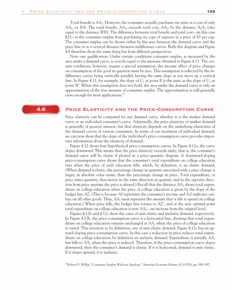
Note one qualification: Under certain conditions consumer surplus, as measured by thearea under a demand curve, is exactly equal to the measure obtained in Figure 4.11. The cer-tain conditions, however, require a special assumption: the income effect of price changeson consumption of the good in question must be zero. This assumption is reflected by the in-difference curves being vertically parallel, having the same slope as you move up a verticalline. In Figure 4.11, for example, the slope of U1 at point R is the same as the slope of U2 atpoint W. When this assumption does not hold, the area under the demand curve is only anapproximation of the true measure of consumer surplus. The approximation is still generallyclose enough for most applications.11
4.6 Price Elasticity and the Price-Consumption Curve
Price elasticity can be computed for any demand curve, whether it is the market demandcurve or an individual consumer’s curve. Admittedly, the price elasticity of market demandis generally of greatest interest, but that elasticity depends on the underlying elasticities ofthe demand curves of various consumers. In terms of our treatment of individual demand,we can now show that the slope of the individual’s price-consumption curve provides impor-tant information about the elasticity of demand.
Figure 4.12 shows four hypothetical price-consumption curves. In Figure 4.12a, the curveslopes downward. This means that the price elasticity exceeds unity; that is, the consumer’sdemand curve will be elastic if plotted in a price–quantity diagram. A downward-slopingprice-consumption curve shows that the consumer’s total expenditure on college educationrises when the price of such education falls, which, by definition, is an elastic demand.(When demand is elastic, the percentage change in quantity associated with a price change islarger, in absolute value terms, than the percentage change in price. Total expenditure, orprice times quantity, thus moves in the same direction as quantity and in the opposite direc-tion from price anytime the price is altered.) Recall that the distance AA1 shows total expen-diture on college education when the price of college education is given by the slope of thebudget line AZ. (This is because A0 represents the consumer’s income and A10 indicates out-lays on all other goods. Thus, AA1 must represent the amount that is left to spend on collegeeducation.) When price falls, the budget line rotates to AZ�, and at the new optimal pointtotal expenditure on college education is now AA2—an increase from the original level.
Figures 4.12b and 4.12c show the cases of unit elastic and inelastic demand, respectively.In Figure 4.12b, the price-consumption curve is a horizontal line, showing that total expen-diture on college education remains unchanged at AA1 when the price of college educationis varied. This situation is, by definition, one of unit elastic demand. Figure 4.12c has an up-ward-sloping price-consumption curve. In this case a reduction in price reduces total expen-diture on college education, by definition an inelastic demand. Expenditure is initially AA1
but falls to AA2 when the price is reduced. Therefore, if the price-consumption curve slopesdownward, then the consumer’s demand is elastic. If it is horizontal, demand is unit elastic.If it slopes upward, it is inelastic.
• Price Elasticity and the Price-Consumption Curve 103
11Robert D. Willig, “Consumer Surplus Without Apology,” American Economic Review, 65 (1976), pp. 589–597.

104 Chapter Four • Individual and Market Demand •
Finally, Figure 4.12d shows a U-shaped price-consumption curve. The elasticity of de-mand varies along this curve. It is elastic along the negatively-sloped AJ portion of thecurve; becomes unit elastic at point J, where the slope of the curve is zero; and is inelasticalong the upward-sloping portion of the curve to the right of point J. This type of price-consumption curve is probably typical. It begins at point A because at a high enough priceno college education would be purchased. Thus, it must be negatively-sloped at relativelyhigh prices (implying an elastic demand). On the other hand, there will generally be a finitequantity the consumer would consume even at a zero price, so the price-consumption curvemust slope upward at relatively low prices (implying an inelastic demand). Therefore, a con-sumer’s demand curve tends to be elastic at high prices and inelastic at low prices. Thisknowledge does not help us determine elasticity at a specific price because we don’t knowwhether that specific price is “high” or “low” in this sense.
Collegeeducation
P-C curve
(a)
Z Z′
A
A1
A2
U2
U1
0 Collegeeducation
P-C curve
(b)
Z Z′
A
A1
U2U1
0
Collegeeducation
P-C curve
(c)
Z Z′
A
A2
A1U2
U1
0 Collegeeducation
P-C curve
(d)
U2U1
J
0 Z Z′
Othergoods
Othergoods
Othergoods
A
Othergoods
Price-Consumption Curves and the Elasticity of DemandThe slope of a consumer’s price-consumption curve tells us whether demand is elastic,inelastic, or unit elastic. (a) When the price-consumption curve is negatively-sloped,demand is elastic. (b) When it is zero-sloped, demand is unit elastic. (c) When it ispositively-sloped, demand is inelastic. (d) When it is U-shaped, demand is elastic at highprices and inelastic at low prices.
Figure 11.2Figure 4.12

• Network Effects 105
4.7 Network Effects
Until now we have assumed that a particular consumer’s demand for a good is unrelated toother consumers’ demands for the good. However, this need not be the case. To the extentthat an individual consumer’s demand for a good is influenced by other individuals’ pur-chases, there is a network effect. Network effects can be positive or negative. The positivecase, or bandwagon effect, exists whenever the quantity of a good demanded by a particularconsumer is greater the larger the number of other consumers purchasing the same good.The negative case, or snob effect, occurs when the quantity of a good demanded by a partic-ular consumer is smaller the larger the number of other consumers purchasing the samegood.
The Bandwagon EffectCapitalizing on bandwagon effects is critical to the marketing of some goods. For example,clothing, toy, and food manufacturers realize that their ability to sell certain products to aparticular consumer will be enhanced the greater the number of other consumers purchas-ing the same products. Tommy Hilfiger jeans, Barbie dolls, Pokémon cards, Nike runningshoes, and Evian water are all products characterized by such positive network effects. Insome cases, the positive network effects stem from consumers’ desires to be in fashion andthe utility derived from owning popular products. In other cases, a bandwagon effect de-rives from the fact that the inherent value of a good to a consumer is enhanced by wide-spread usage of the good among other consumers. Take the case of America Online(AOL). The value of AOL to an individual consumer is increased when other consumersalso use AOL if a larger customer base leads to more services, chat rooms, and e-mail con-tacts. The extent of a business school’s alumni network similarly can increase the value ofattending the school to a particular applicant. This is because a greater number of alumstranslates into more connections when the applicant searches for a job after graduating.
Figure 4.13 depicts the case of a bandwagon effect. If consumers believe that only 1,000people own a good, the demand curve is d1,000. If consumers believe that more people own
network effectsthe extent to which anindividual consumer’sdemand for a good isinfluenced by otherindividuals’ purchases
bandwagoneffecta positive network effect
snob effecta negative network effect
Application 4.7
igarettes are among the leading non-politicallycorrect goods and are fair game, consequently, for
many legislators and attorneys. Indeed, juries haveslapped tobacco companies with several multibillionpunitive damages verdicts in recent years. However,the effect on company profits has been less significantthan commonly assumed.12 The adverse effect on prof-its has been mitigated partly through payment of thedamages being made over a long period of time. For in-stance, in 1998 cigarette makers settled suits brought
C by the attorneys general of all 50 states by agreeing topay the huge-sounding sum of $246 billion. For reasonsthat we will explain in a later chapter, however, thereal cost of these damages is much smaller because thebill is due in installments over 25 years.
More importantly, the effect of the verdicts on profitshas been lessened by the ability of companies to raisethe extra revenue they need to pay the damages by rais-ing prices. Because the demand for cigarettes is esti-mated to be inelastic (between 0.3 and 0.5), therelevant P-C curve is upward-sloping as in Figure 4.12c,and total expenditures made by consumers on cigarettesincrease as the price of cigarettes is raised.
12“Yes, $145 Billion Deals Tobacco a Huge Blow, But Not a KillingOne,” Wall Street Journal (July 17, 2000), pp. A1 and A8.
Application 4.7 The P-C Curve for a non-PC Good

106 Chapter Four • Individual and Market Demand •
the good and, consequently, the good is more desirable—either because it is in greater fash-ion or because its inherent value is increased—the demand curve is located farther to theright at any price: d2,000 if 2,000 people are believed to own the good; d3,000 if 3,000 peopleare believed to own the good; and so on.
With a bandwagon effect, the market demand curve, D, is more price elastic. To see why,suppose that consumers initially are willing to purchase 1,000 units if the price is $50. Nowconsider a decrease in price from $50 to $40. Without any bandwagon effect, the quantitydemanded would increase to 1,250 along curve d1,000. The bandwagon effect, however, re-sults from more people purchasing the good at the lower price, and this, in turn, increasesthe willingness of consumers to purchase the good for its greater fashion or inherent value.
In the case of Figure 4.13, 2,000 units are purchased at a price of $40, and the bandwagoneffect accounts for the increase in quantity demanded from 1,250 to 2,000 in response to thedecrease in price from $50 to $40. The market demand curve is derived by connecting thepoints on the curves d1,000, d2,000, and d3,000 corresponding to the quantities 1,000, 2,000, and3,000. A, B, and C are the only points consistent with the expected quantities associatedwith each of the curves. By contrast, point E, representing a quantity of 1,250 on the curved1,000, is inconsistent with consumers’ beliefs that overall purchases total 1,000 units andthus cannot lie on the market demand curve.
The market demand curve is more elastic that the individual curves d1,000, d2,000, and d3,000
because the bandwagon effect increases the response in quantity demanded to any change inprice. In other words, the total response in quantity demanded to a change in price is thesum of the pure price effect and the bandwagon effect. Thus, it exceeds the pure price effectin magnitude.
The Snob EffectThe snob effect is the opposite of the bandwagon effect. It occurs when a consumer is lesswilling to purchase a good the more widespread its usage. A vintage Jaguar car, an originalcopy of the Declaration of Independence, a custom-made Versace evening gown, a Picassopainting, and a hand-crafted Piaget watch are all possible examples of goods associated with
Quantity
C
B
A
E
D
$40
$50
0
Price
d1,000 d2,000 d3,000
1,000 1,250 2,000 3,000
band-wagoneffect
purepriceeffect
Figure 4.13Figure 4.13
Bandwagon EffectA bandwagon effect leads to greater consumerpurchases of a good the more other consumersare believed to desire the same good. The marketdemand curve, D, is more elastic because thebandwagon effect increases the response inquantity demanded to any change in price.

• Network Effects 107
snob effects. A consumer’s valuation of such goods may be greater the more exclusive arethe goods, on account of the prestige and admiration derived by the consumer from thegoods being selectively owned.
Figure 4.14 depicts a snob effect in the case of vintage Jaguar cars. The relevant demandcurves are d10, d20, and d30 if consumers believe that only 10, 20, and 30 people, respectively,own a particular model. Note that the demand curve is farther to the right at any givenprice the more exclusive the ownership of the vintage Jaguar model is believed to be—d20 isto the right of d30 and d10 is to the right of d20. This reflects a snob effect: the quantity of agood demanded by a particular individual falls the more widely owned the good is consid-ered to be by other consumers.
The market demand curve is more inelastic in the case of goods characterized by a snobeffect. To see why, note that the market demand curve connects the points on curves d10,d20, and d30 associated with the quantities 10, 20, and 30. F, G, and H are the only pointsconsistent with the expected purchases associated with curves d10, d20, and d30. Point I can-not lie on the market demand curve because a quantity of 5 is inconsistent with the expec-tation of 30 purchases associated with d30.
An alternative, and perhaps clearer, way of understanding why the market demand curveis more inelastic in the case of goods characterized by a snob effect is to examine the effectof a price increase, such as from $50,000 to $150,000 in Figure 4.14. The pure price effect ofthis increase decreases consumption from 30 to 5 vintage Jaguar cars along curve d30. How-ever, the snob effect associated with the enhanced exclusivity resulting from the price in-crease works to counteract the pure price effect and increases consumption from 5 to 20units. On net, therefore, the price increase leads to a decrease in the quantity demand from30 to only 20 units and is less than the decrease associated with the pure price effect. Be-cause the snob effect runs counter to the pure price effect, the market demand curve is lessprice elastic—the cumulative impact of the pure price and snob effects on quantity de-manded is less than the pure price effect.
Quantity
G
H
D
F
I
$50,000
$150,000
0
Price
d30
d10
d20
205 10 30
snobeffect
pure price effect
Figure 4.14Figure 4.14
Snob EffectA snob effect leads to smaller consumer purchasesof a good the more other consumers are believedto desire the same good. The market demandcurve, D, is less elastic because the snob effectdecreases the response to quantity demanded forany change in price.

Application 4.8
ommunications technologies are prime examplesof products characterized by positive network ef-
fects.13 As the established user base of telephones‚ faxmachines‚ the Internet‚ and e-mail grows‚ increasinglymore individuals find adoption worthwhile. Conse-quently‚ such products tend to be characterized by rela-tively long developmental periods followed by rapiddiffusion. Take the case of fax machines‚ a product thatAT&T introduced an introductory version of in 1925.The technology‚ however‚ was little used until the mid-1980s‚ when demand for and supply of fax machines ex-ploded. While ownership of fax machines was negligibleprior to 1982‚ over half of American businesses had atleast one fax machine by 1987.
Internet usage has followed a similar pattern. Whilethe first email message was sent in 1969‚ Internet trafficdid not begin to grow substantially until the late 1980s.Once it began to grow‚ however‚ it doubled annually invirtually every year after 1989.
Positive network effects are not limited to communi-cations technologies. They are also at the heart of ex-plaining the diffusion of computer software and hardware‚where popular systems enjoy a significant competitiveadvantage over less popular systems. Personal computersprovide a telling example. A study of 110‚000 Americanhouseholds in 1997 suggests that the rate of adoption ofpersonal computers may have been almost doubled onaccount of network effects. Moreover‚ the observed net-work effects are strongly related to usage of the Internetand e-mail.
Positive network effects also likely have played animportant role in the rapid spread of popular computer
C
108 Chapter Four • Individual and Market Demand •
Application 4.8 Network Effects and the Diffusionof Communications Technologiesand Computer Hardware and Software
13This application is based on Carl Shapiro and Hal R. Varian‚ Infor-mation Rules (Boston: Harvard Business School Press‚ 1999); and Aus-tan Goolsbee and Peter J. Klenow‚ “Evidence on Learning andNetwork Externalities in the Diffusion of Home Computers‚” Journalof Law and Economics‚ 45 No. 2 Pt. 1 (October 2002), pp. 317–343.
software programs such as Microsoft’s Windows operat-ing system and Office (a combination of word process-ing‚ spreadsheet‚ data base‚ and presentation programs).Both products quickly acquired shares of over 90 percentof their relevant markets.
Of course‚ the same positive network effects pro-pelling a product’s rapid diffusion can also have adverselegal consequences. For example‚ the Justice Depart-ment’s antitrust case against Microsoft hinged criticallyon the positive network effects fueling Window’ssuccess.
The Justice Department alleged that a positive net-work effect allowed Microsoft to capture a dominantshare of the personal computer operating system market.In turn, the built-in customer base gave Microsoft a sig-nificant edge in the browser market for its Internet Ex-plorer product over rival Netscape Navigator, said theJustice Department, because, at no extra charge to con-sumers, Microsoft packaged Internet Explorer with itsWindows operating system.
We will explore the Microsoft antitrust case morefully in Chapter 11, but one point that deserves mentionhere is that positive network effects can be a two-edgedsword for suppliers. Although a bandwagon effect en-hances the possibility that a supplier will capture a dom-inant market share, it simultaneously limits thesupplier’s ability to exploit that position through a priceincrease. As we saw in Figure 4.13, the market demandcurve is more price elastic when there are positive net-work effects present. In the case of Windows, this im-plies that Microsoft’s ability to exploit, through a priceincrease, the dominant customer base that a bandwagoneffect helped to build is limited by the same bandwagoneffect. Should Microsoft attempt to raise Windows’price, customers would run toward alternative operatingsystems more quickly than they would without thebandwagon effect being present.

4.8 The Basics of Demand Estimation
Although indifference curves and budget lines together provide an appealing theoreticalmodel of consumer choice, our ability to test the validity of the model and apply it to thereal world rests critically on the extent to which we are able to empirically estimate individ-ual consumers’ or market demand curves. There are three methods generally relied upon toestimate demand. These are experimentation, surveys, and regression analysis. We brieflyoutline each of these methods as well as their accompanying pitfalls.
ExperimentationMcDonald’s will often run a controlled experiment to test how the demand for one of itsfast-food items responds to a change in its price or to a change in the price of a complement.For example, McDonald’s will select a number of franchises at which the price of french friesis lowered to determine the effect of such a change on Big Mac sandwich sales. Based on theresults, the managers can estimate the sensitivity of Big Mac demand to the price of thecomplement, french fries, and thereby derive a relevant cross-price elasticity of demand.
While a valid mechanism for estimating demand, experimentation carries with it somelimitations. Among these is that to run a true, controlled experiment, only one determi-nant, such as the price of french fries, should be changed at a time to determine its impacton Big Mac sales. Suppose that the price charged by Burger King for its products rises or thelocal income level falls at the same time that the McDonald’s french fries price is altered. Ifthis is the case, McDonald’s managers will get a contaminated and unreliable measure of theimpact of the price of their french fries on Big Mac sales.
Another limitation is one of generalizability. It may be incorrect to assume that the ex-perimental results obtained in one sample of McDonald’s franchises apply to all. The effecton Big Mac sales of a change in the price of french fries may be much different in Ohio thanin Osaka, Japan. Experimental results from a sample of Ohio franchises thus may not gener-alize to those in Osaka.
SurveysTo anticipate the market reaction to a price increase, the Ford Motor Company regularlyconducts consumer surveys—either by mail, telephone, or focus groups. A Californian willbe contacted by telephone, for instance, and asked about the extent to which her likelihoodof purchasing a Taurus automobile over the next 12 months will be diminished if the price israised by $400.
As with experimentation, customer surveys can generate valuable information. They arenot, however, foolproof. As with experimentation, one must be careful to choose a represen-tative sample. A good example of what can happen if this rule is not heeded involves one ofthe first U.S. presidential polls—a survey taken prior to the 1936 election that predicted Re-publican Alf Landon would crush Democrat Franklin Delano Roosevelt. The exact oppositeoccurred. The poll surveyed citizens whose names had been taken from telephone directo-ries and automobile registration rolls. Since the rich were more likely to have telephonesand cars in 1936 and were also more likely to be Republican, the poll was based on a non-representative sample of the voting population.
Furthermore, a survey’s reliability is dependent on respondents telling the truth. For ex-ample, there is considerable evidence that polls will not accurately predict election resultswhere political candidates and voters are of different ethnic backgrounds. While those sur-veyed say they will vote for a candidate whose ethnicity is different from their own, once inthe privacy of the voting booth they are more likely to pull the lever for a candidate similarto themselves.
• The Basics of Demand Estimation 109
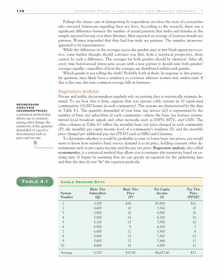
110 Chapter Four • Individual and Market Demand •
Perhaps the classic case of misreporting by respondents involves the story of a researcherwho surveyed Americans regarding their sex lives. According to the research, there was asignificant difference between the number of sexual partners that males and females in thesample reported having over their lifetimes. Men reported an average of fourteen female sexpartners. Women responded that they had four male sex partners. The samples, moreover,appeared to be representative.
While the difference in the averages across the genders may at first blush appear provoca-tive, some further thought should convince you that, from a statistical perspective, therecannot be such a difference. The averages for both genders should be identical. After all,every time heterosexual intercourse occurs with a new partner it should raise both genders’averages equally—regardless of how the averages are distributed within each gender.
Which gender is not telling the truth? Probably both of them. In response to this particu-lar question, men likely have a tendency to overstate whereas women may undercount. Ifthis is the case, the true, common average falls in between.
Regression AnalysisPrivate and public decisionmakers regularly rely on existing data to statistically estimate de-mand. To see how this is done, suppose that you operate cable systems in 10 equal-sizedcommunities (10,000 homes in each community). The systems are characterized by the datain Table 4.1. The quantity demanded of your basic tier service (Q) is represented by thenumber of basic tier subscribers in each community—where the basic tier features retrans-mitted local broadcast signals and other networks such as ESPN, MTV, and CNN. Theother columns in Table 4.1 reflect the monthly basic tier price charged in each community(P), the monthly per capita income level of a community’s residents (I), and the monthlyprice charged per additional pay tier (PPAY) such as HBO and Cinemax.
To determine whether it would be profitable to raise or lower basic tier prices, you wouldwant to know how sensitive basic service demand is to its price, holding constant other de-terminants such as per capita income and the pay tier price. Regression analysis, also calledeconometrics, is a statistical method that allows you to estimate this sensitivity based on ex-isting data. It begins by assuming that we can specify an equation for the underlying dataand that the data do not “fit” the equation perfectly.
Table 4.1 Cable Demand Data
Basic Tier Basic Tier Per Capita Pay TierSystem Subscribers Price Income PriceNumber (Q) (P) (I) (PPAY)
1 3,300 $18 $3,900 $222 6,600 10 5,560 103 3,900 18 8,900 184 5,000 14 8,200 165 5,100 15 7,950 106 6,900 9 6,500 77 6,400 12 5,900 88 5,900 13 7,500 159 5,800 12 7,864 12
10 4,800 18 4,500 12
Average 5,370 $13.90 $6,677.40 $13
regressionanalysis(econometrics)a statistical method thatallows one to estimate,among other things, thesensitivity of the quantitydemanded of a good todeterminants such asprice and income

• The Basics of Demand Estimation 111
Take the case of the information in Table 4.1. Let us start by supposing that only P influ-ences Q and that the demand for basic cable in a community is best described by the follow-ing linear relationship:
Qi � a � bPi � ei; (1)
where the subscript i refers to the number of the system or the “observation” being consid-ered. The variable Q that the equation is seeking to explain is called the dependent vari-able. Any variable such as P employed to explain the dependent variable is called anexplanatory variable. The error term, e, is included in the equation to account for eithermistakes in data collection; determinants of demand other than P that are inadvertently or,due to a lack of data, intentionally omitted from the relationship; or the possibility that thedemand for basic cable is, to a certain extent, random and thus not predictable by economicmodels. The term a is the intercept of the linear equation—the number of subscribers a sys-tem will have if the basic price and the error term equal zero. And b, the coefficient on thebasic tier price, indicates by how much the number of subscribers will change per dollarchange in the basic tier price (b � �Q/�P).
Regression analysis usually employs the ordinary least-squares or OLS technique to esti-mate equations such as the one we have specified for the demand for basic cable. OLS esti-mates the “best fitting” intercept and coefficient for the specified relationship and theemployed data. Best fitting means that the estimated equation will be “as close as possible” tothe observed data points. The technical criterion for “as close as possible” involves the dis-tances between the various data points and the estimated equation.
The specific manner in which OLS determines the equation that best fits the data is be-yond the scope of this book.14 Suffice it to say that the intercept and coefficient estimated byOLS (where estimated is signified with a “∧” as in â and b) serves to minimize the distancesbetween the data points and the estimated equation. The distances between the data pointsand the estimated equation represent the errors made by the estimated equation across thevarious data points.
Figure 4.15 graphically depicts how OLS regression works. In the simple demand rela-tionship assumed by equation (1), the intercept and coefficient for the estimated equationthat best fits the data across the ten systems turn out to be â � 9,970.1 and b � �330.9, re-spectively. The intercept estimate â implies that for the sample examined and the demandrelationship assumed, if price were set equal to 0, the forecast number of basic subscribers, Q,would be 9,970.1. The coefficient estimate b means that for every $1 increase in themonthly basic tier price, the number of basic subscribers decreases by 330.9 (b � �Q/�P).The slope of the estimated regression line is �P/�Q and thus equals 1/b � �0.003.
The dots in Figure 4.15 represent the actual prices and quantities of the 10 systems in oursample. For the tenth system, for example, the price, P10, is $18 and the number of basic sub-scribers, Q10, is 4,800. The OLS-estimated number of basic subscribers for the tenth system,Q10, is equal to the value obtained for Q when one plugs in the tenth system’s price into theestimated regression line. Thus, Q10 � 9,970.1 � 330.9(18) � 4,013.9. The error made byOLS in estimating demand for the tenth system, ê10, is the difference between the actualand forecast number of basic subscribers and equals 786.1 (Q10 � Q10 � ê10 � 786.1). TheOLS regression has calculated â and b so as to minimize the sum of the squares of such errorsacross the ten systems in the sample. From the perspective of Figure 4.15, OLS positions theregression line, â � bPi, so as to best fit the scatterplot of data points—where the “fit” reflectsthe horizontal distances of the observed data points from the estimated equation.
14Most beginning econometrics texts explore the derivation of the intercept and coefficients through OLS in con-siderable detail. So long as you understand the intuition behind their derivation, that will suffice for the material inour book.
ordinary least-squares (OLS)a technique for estimatingthe equation that “bestfits” the data

112 Chapter Four • Individual and Market Demand •
The estimated OLS equation provides valuable demand-side information. For instance, ifwe wanted to calculate the elasticity of demand for basic cable service at the average basictier price and number of basic subscribers in our sample we would use the now-familiar for-mula:
h � (�Q/�P)
where and are the average basic tier price and number of subscribers, respectively, forthe sample. The first part of the right-hand side of the elasticity formula, �Q/�P, is the rateat which the number of a system’s subscribers changes per dollar change in the basic price.This is none other than the b or �330.9 estimated by OLS. Employing the average valuesfor P and Q reported in Table 4.1, one obtains an elasticity of demand of 0.9. Since this isless than unity, demand for basic cable is inelastic when evaluated at the price and numberof subscribers for the average system in the sample. This indicates that profit could be in-creased by raising the average basic price.
Suppose that we estimated a more extensive basic cable demand relationship, such as:
Qi � a � bPi � cIi � dPPAYi � ei. (2)
This more extensive model tries to control explicitly for more of the factors that mightaffect demand for basic cable. OLS regression proceeds in a fashion analogous to the oneemployed in estimating the simpler equation (1). OLS calculates the intercept â and coeffi-cients b, c, and d so as to best fit the observed data—now incorporating information on in-come, I, and the price of pay tier service, PPAY, in the estimation process. In this moreextensive model, the estimated coefficient c measures the independent effect of a $1 in-crease in per capita income on the number of basic subscribers in a community. Its value in-dicates whether basic cable is a normal or an inferior good across the systems in the sample.The estimated coefficient c associated with the pay tier price variable, PPAY, reflects theimpact of a $1 increase in the pay tier price on the demand for basic cable, holding constantthe basic tier price and the per capita income level. It tells us whether pay service is a com-plement or substitute for basic cable in our sample of systems.
QP
(P/Q);
Q
$18
0
P
$30.13
4,013.9
Q10
error10 = 786.1
4,800
Q10
Qi = a + bPi
a = 9,970.1
Point for system 10
Slope = 1/b = – 0.003
$1330.9
⟩
⟩
Figure 4.15Figure 4.15
Ordinary Least-Squares RegressionOrdinary least-squares positions theregression line, Qi � â � bPi, so as to “bestfit” the sample data points.

Application 4.9
cDonald’s makes extensive use of regressionanalysis in determining where to locate fran-
chises. Sales are estimated for any possible location as afunction of factors such as the prices that will becharged; demographics (including the surrounding com-munity’s income level, average family unit size, and eth-nic composition); the availability of substitutes; trafficflows; and the side of the street on which the franchisewill be located (sales are higher if a franchise is on the
M side of the street with the heaviest home-bound traffic atday’s end).
By contrast, McDonald’s rival Burger King has asmaller demand forecasting staff and often relies on a dif-ferent, much simpler mechanism for determining franchiselocations. Burger King waits for McDonald’s to make thefirst move. After McDonald’s statistically determines thata location will be profitable and begins operations on thatsite, Burger King opens up its own franchise nearby.
• Summary 113
Controlling explicitly for more variables can affect the estimate of the effect of basicprice on the demand for basic service. When equation (2) is estimated, â � 9,931.0, b � �230.0, c � �0.01, and d � � 99.5. By comparison, the estimated basic price coeffi-cient, b, was larger in magnitude when equation (1) was used. Use of equation (2) ratherthan equation (1) causes the estimated demand elasticity to fall as well. This is probably atruer estimate of the elasticity because it controls for additional causal factors.
We close this chapter by noting that while regression analysis is a powerful tool allow-ing one to estimate the effects of individual determinants on demand while holding con-stant other determinants’ effects, it also has its difficulties. For one, the intercepts andcoefficients estimated by OLS regression are only as good as the data and the models towhich the analysis is applied. “Garbage in, garbage out,” as the saying goes. If the sampledata are nonrepresentative of the larger population or if the assumed demand relationshipis incorrect (for example, linear when it should be nonlinear), unreliable estimates willresult.
Application 4.9 Demand Estimation: McDonald’s Versus Burger King
Summary
• By rotating the budget line confronting a consumer,we can determine the market basket the consumer will se-lect at different prices, while factors such as income, pref-erences, and the prices of other goods are held constant.The various price–quantity combinations identified inthis way can be plotted as the consumer’s demand curve.• To determine whether a demand curve must have anegative slope, we separate the effect of a change in priceon quantity demanded into two components, an incomeeffect and a substitution effect.• For a normal good, both income and substitutioneffects imply greater consumption at a lower price. Thus the demand curve for a normal good must slopedownward.
• For an inferior good, the income and substitution ef-fects of a price change operate in opposing directions. Ifthe income effect is larger, the demand curve will slopeupward. However, both theoretical reasoning and empiri-cal evidence suggest this case is quite rare.• Consumer surplus is a measure of the net benefit aconsumer receives from consuming a good. It is showngraphically by the area between the consumer’s demandcurve and the price line.• Consumer surplus can also show the benefit or cost aconsumer receives as a result of a change in the price ofthe good.• Individual consumers’ demand curves can be aggre-gated to obtain the market demand.

114 Chapter Four • Individual and Market Demand •
• The price-consumption curve provides important in-formation about an individual’s elasticity of demand.• An individual consumer’s purchases of a good may beinfluenced by other individuals’ purchases through net-work effects.
• Three methods allow us to estimate individuals’ ormarket demand curves: experimentation, surveys, and re-gression analysis or econometrics.
Review Questions and Problems
Questions and problems marked with an asterisk have solutions givenin Answers to Selected Problems at the back of the book (pagesxxx–xxx).
4.1. Explain how the indifference curve and budget line appa-ratus are used to derive a consumer’s demand curve. For a de-mand curve, certain things are held constant. What are they,and how does this approach hold them constant?
4.2. If the per-unit price of college education rises and theprices of all other items fall, is it possible for the consumer toend up on the same indifference curve as before the pricechanges? If so, will the consumer be purchasing the same marketbasket? Support your answer with a diagram.
4.3. “A Giffen good must be an inferior good, but an inferiorgood need not be a Giffen good.” Explain this statement fully,using the concepts of income and substitution effects.
*4.4. Assume that Joe would like to purchase 50 gallons ofgasoline monthly at a price of $1.50 per gallon. However, the$1.50 price is the result of a government price ceiling, sothere is a shortage, and Joe can only get 25 gallons. Showwhat this situation looks like by using indifference curves anda budget line. Then, show that Joe will be willing to pay aprice higher than $1.50 to get additional units of gasoline.(This result is the demand-side reason for the emergence of ablack market.)
4.5. Delores has a different price-consumption curve associatedwith each possible income level. If two of these curves intersect,are Delores’ preferences rational?
*4.6. If Edie’s income rises by 50 percent and, simultane-ously, the price of automobile maintenance increases by 50percent, can we predict how Edie’s consumption of automo-bile maintenance will be affected? Can we predict how, on av-erage, Edie’s consumption of other goods will be affected? Usethe concepts of income and substitution effects to answer thisquestion.
4.7. Assume that Dan’s income-consumption curve for pota-toes is a vertical line when potatoes are on the horizontal axis.Show that Dan’s demand curve for potatoes must be downward-sloping.
4.8. Given the OLS estimates for the coefficient and interceptin the basic tier cable demand equation (1), calculate the pointdemand elasticity for system number 7.
4.9. Given the OLS estimates for the coefficients and interceptin the basic tier cable demand equation (2), calculate the fol-lowing:a. Income elasticity of demand for basic service evaluated at
the average values for monthly per capita income and thenumber of basic subscribers across the sample of ten systems.Based on your calculation, is basic cable a normal or an infe-rior good?
b. Cross-price elasticity of demand for basic service with re-spect to the pay tier price evaluated at the average valuesfor the pay tier price and the number of basic subscribersacross the 10 systems in the sample. Based on your calcula-tion, is pay tier service a substitute or a complement forbasic service?
c. The income elasticity of demand for basic service evaluatedat the income and quantity data for system number 3.
4.10. Suppose that Lorena consumes only three differentgoods: steak knives, butter knives, and butcher knives. If, ac-cording to Lorena’s preferences, butter and butcher knives areinferior goods, must steak knives be a normal good? Explain youranswer.
4.11. Suppose that there are only five consumers of a softwaregame program. The demand curve for each of the consumers isidentical. Will the market demand curve that is obtained byhorizontally summing across the five individual consumers’ de-mand curves be less or more price elastic at any price than thedemand curve for any of the individual consumers?
4.12. Suppose that the Downtown Athletic Club increases itsmonthly membership charge from $150 to $200. Among thebusinesspeople belonging to the Club, would you expect lower-level business managers to be more sensitive to the price in-crease than senior managers? Explain using indifference curves.
4.13. Suppose that George is interested in only two goods, cig-ars and scotch. Employ the indifference curve/budget line appa-ratus to show a case where a decrease in the price of cigars leadsto an increase in George’s scotch consumption. Does this implythat cigars and scotch are complements to George? Explain youranswer.
4.14. Repeat the preceding question but assume that a decreasein the price of cigars leads to a decrease in George’s scotch con-sumption. Does this imply that scotch is an inferior good inGeorge’s case?

• Review Questions and Problems 115
4.15. In the tax-plus-rebate example discussed in the text, sup-pose that the government adjusts the size of the rebate so thatthe consumer stays on her initial indifference curve (U2 in Fig-ure 4.4). Show the results in a diagram. Can the governmentachieve this result for all consumers? Why or why not?
*4.16. When the price of gasoline in Italy is $5 per gallon,Fabio consumes 1,000 gallons per year. The price rises to $5.50and, to offset the harm to Fabio, the Italian government giveshim a cash transfer of $500 a year. Will Fabio be better or worseoff after the price rise plus transfer? What will happen to hisgasoline consumption?
4.17. Left and right shoes are perfect complements for mostpeople. If only the price of right shoes increased, what would bethe substitution effect of such a price change on the typical con-sumer’s consumption of right shoes (assume that the only twogoods that the consumer cares about are right and left shoes)?What about the income effect?
4.18. If Clint’s elasticity of demand for cigars is equal to zero,are cigars a normal or an inferior good for Clint? Explain.
4.19. Define consumer surplus, and explain how you wouldshow it in a diagram containing a demand curve for some prod-uct. What would consumer surplus equal in Figure 4.8 if the de-mand was perfectly elastic at the market price of $3 per espressocup?
4.20. Diamonds clearly satisfy less important needs than water,which is essential to life. Yet according to market prices, the es-sential commodity, water, is worth less than the less essentialcommodity, diamonds. Why would a vital commodity such aswater sell for so much less than diamonds? Does this imply thatthere is something wrong with a market system that values dia-monds more than water? Explain using demand and supplycurves for water and diamonds. In your explanation, distinguishbetween the marginal and total benefit of the two commodities.
4.21. Noneconomists sometimes refer to medical care as “in-valuable” or “priceless.” Do you think these terms may be simplyimprecise ways of saying that the consumer surplus associatedwith medical care is very large? Suppose that the consumer sur-plus is immense. Explain why this is irrelevant in decidingwhether to provide more medical care. What is relevant?
4.22. “The price of water is a measure of water’s marginal bene-fit to consumers.” Is this statement true for all consumers ofwater? If a government price ceiling is set below the equilibriumprice, will the price equal the marginal benefit of water?
4.23. Could the snob effect ever overpower the combined sub-stitution and income effects associated with an increase in theprice of a good? Explain why or why not.
4.24. Explain how a bandwagon effect might speed up the rateat which DVD players are adopted by consumers. Do likewisefor the case of cable television subscriptions.
4.25. Suppose that the P-C curve associated with a pharmaceu-tical drug is downward-sloping. If the government underwrites acertain percentage of consumers’ drug purchases, will the govern-ment outlays associated with such a program be greater the largerthe percentage of the purchases underwritten? Explain why orwhy not. What if the P-C curve is upward-sloping?
4.26. During the 1970s, 55 percent of banks with more than 15branches installed atomated teller machines (ATMs), as opposedto 16 percent of banks with only 2 branches. Explain why thisphenomenon attests to the presence of positive network effects.
4.27. If the price of hamburger is increased and a consumer’squantity demanded of hamburger decreases‚ the income effect issmaller than the substitution effect. True‚ false, or uncertain?Explain.
4.28. Every market generates at least some consumer surplusand the amount generated depends critically on the prevailingprice. True‚ false, or uncertain? Explain.