Chapter 4
103
Chapter 4 Tensors in Generalized Coordinates in Three Dimensions 1. Coordinate Curves and Coordinate Surfaces R ectilinear coordinates in three dimensions have been defined in terms of three non-coplanar straight lines which intersect in a common point, the origin. The three lines are the coordinate axes. Taken by pairs, these axes also define the coordinate planes. Thus in Cartesian coordinates we have the mutually perpendicular and axes which define the and planes. Along each axis, one coordinate varies, the other two are zero. The axes may therefore be called coordinate curves. In the coordinate planes, one coordinate is fixed, the other two vary. The planes are therefore called coordinates surfaces. More generally, we see that the lines defined by (1) (2) and (3) form a triply infinite family of coordinate curves which fill all of three-dimensional Euclidean space. Associated with them is the triply infinite family of planes (1) and (3) If the lines or planes are mutually orthogonal, the coordinate system is Cartesian; otherwise it is merely rectilinear. Let us now waive the condition that the coordinate surfaces need be planes. Let them be simply any triply infinite families of surfaces such that (1) each family fills all of space or at least all of that region of space which is of interest and (2) the members of any one of the three families do not intersect others of the same family but do intersect members of the other families. In that event, any point of space may be located as being at the mutual intersection of three particular coordinate surfaces. The parameters of the three particular surfaces are the generalized coordinates of the point in question. The intersections of the coordinate surfaces by pairs define the three coordinate curves. They thus consist of three families of curves such that one and only one member of each family passes through each point of space. As an example, consider the familiar spherical coordinate system. The coordinate surfaces are (1) all spheres about the origin, (2) all right circular cones with a common axis and a common vertex at the origin, and (3) all planes through the cones’ common axis (see Fig. 71). The coordinate curves are (1) all straight lines through the origin (radii), (2) all circles with centers on the axis and planes perpendicular to the axis (parallels of latitude), and (3) all circles with center at the origin and diameters along the axis (meridians of longitude). As was the case in two dimensions, generalized or curvilinear coordinates are themselves not vector components, in general. Though every set of coordinates locates a point of space uniquely, those coordinates are in general not the components of a
Transcript of Chapter 4
Chapter 4
Tensors in Generalized Coordinates in Three Dimensions
1. Coordinate Curves and Coordinate Surfaces
Rectilinear coordinates in three dimensions have been defined in terms ofthree non-coplanar straight lines which intersect in a common point, the origin. The
three lines are the coordinate axes. Taken by pairs, these axes also define the coordinateplanes. Thus in Cartesian coordinates we have the mutually perpendicular and
axes which define the and planes. Along each axis, one coordinatevaries, the other two are zero. The axes may therefore be called coordinate curves. Inthe coordinate planes, one coordinate is fixed, the other two vary. The planes aretherefore called coordinates surfaces.
More generally, we see that the lines defined by (1) (2) and (3) form a triply infinite family of coordinate
curves which fill all of three-dimensional Euclidean space. Associated with them is thetriply infinite family of planes (1) and (3) If the linesor planes are mutually orthogonal, the coordinate system is Cartesian; otherwise it ismerely rectilinear.
Let us now waive the condition that the coordinate surfaces need be planes. Let thembe simply any triply infinite families of surfaces such that (1) each family fills all ofspace or at least all of that region of space which is of interest and (2) the members ofany one of the three families do not intersect others of the same family but do intersectmembers of the other families. In that event, any point of space may be located as beingat the mutual intersection of three particular coordinate surfaces. The parameters of thethree particular surfaces are the generalized coordinates of the point in question.
The intersections of the coordinate surfaces by pairs define the three coordinatecurves. They thus consist of three families of curves such that one and only one memberof each family passes through each point of space. As an example, consider the familiarspherical coordinate system. The coordinate surfaces are (1) all spheres about the origin,(2) all right circular cones with a common axis and a common vertex at the origin, and(3) all planes through the cones’ common axis (see Fig. 71).
The coordinate curves are (1) all straight lines through the origin (radii), (2) allcircles with centers on the axis and planes perpendicular to the axis (parallels oflatitude), and (3) all circles with center at the origin and diameters along the axis(meridians of longitude).
As was the case in two dimensions, generalized or curvilinear coordinates arethemselves not vector components, in general. Though every set of coordinates locatesa point of space uniquely, those coordinates are in general not the components of a

1. Coordinate Curves and Coordinate Surfaces 203
position vector to that point. This is one immediate and important distinction betweenrectilinear and curvilinear coordinates. It was on this account, for example, that theequations of motion of rigid bodies, which are extended objects, are more easily treatedin rectilinear coordinates. On the other hand, various other types of problems are to betreated more conveniently in certain suitably chosen generalized coordinate systems.
Though the coordinates themselves are not position vector components ingeneralized coordinate systems, the differentials of the coordinates invariably are, forif are new coordinates given as functions of old coordinates then
(1.1)
is not only the law of transformation of differentials but the contravariant vectortransformation law as well, where the differential vector is used to find thecomponents in the new coordinate system.
This connection between the transformation of differentials and the transformationlaw for differential vectors is no coincidence. It stems from the fact that at any point Othe tangents to the coordinate curves through that point may be used to define a localrectilinear system (see Fig. 72). The respective coordinate differentials at that pointlie along these rectilinear axes, thus constitute the components of a differentialcontravariant vector. The tangent planes to the coordinate surfaces at O are thecoordinate surfaces of this associated rectilinear system. We may thus define vectors andtensors of every sort in this rectilinear system and subject them to all the definedalgebraic manipulations that were possible in rectilinear systems in general.
Figure 71

Chapter 4: Tensors in Generalized Coordinates in Three Dimensions204
Figure 72
We now associate all vector and tensor quantities defined at O in the tangentrectilinear system with the curvilinear coordinate system itself. Any reversibletransformation of coordinates will at most simply define a new tangent rectilinearsystem at O. Between this and the former system, the usual tensor transformation holds.It is necessary only that the transformation should be reversible at O, for which it is bothnecessary and sufficient that
(1.2)
The operations permitted by the previous argument all had to be performed strictlyat the point O. These include addition, subtraction, multiplication, and the formation ofinner and vector products. Not included was the operation of differentiation, whichrequires the formation of differences of vectors not at the same point. This sameproblem arose in considering curvilinear coordinates in two dimensions and may herebe solved in an exactly analogous manner. The result is formally identical, and leads tothe same definition of intrinsic and covariant differentiation. Hence these operations andassociated formulae will be taken over intact. Only one minor difference need be noted,namely, that the indices of the Christoffel three-index symbols may now be all distinct,an impossibility in two dimensions.

1. Coordinate Curves and Coordinate Surfaces 205
Figure 73
Ex. (1.1) (a) Identify the coordinate curves and coordinate surfaces in acylindrical coordinate system related to a Cartesian coordinate system by the transformations
(b) Find the inverse transformations.
Ans. (a) The curves (see Fig. 73) are any straight lines through the axisand perpendicular to it; the curves are circles about the axis and lyingin a plane perpendicular to the axis; the curves are straight lines parallelto the axis. An surface is a right circular cylinder whose axis is the
axis; an surface is any plane containing the axis; an surface isany plane perpendicular to the axis.

Chapter 4: Tensors in Generalized Coordinates in Three Dimensions206
Figure 74
Ex. (1.2) (a) Identify the coordinates surfaces in a parabolic cylindricalcoordinate system which is related to Cartesian coordinates by thetransformation
(b) Find the inverse transformation.
Ans. (a) Setting (see part (b) below), we have
which is the parametric representation of a family of parabolic cylinders openingto the negative axis. Setting we have

1. Coordinate Curves and Coordinate Surfaces 207
Figure 75
which is the parametric representation of a family of parabolic cylinders openingto the positive axis. Setting gives a plane perpendicular to the
axis.
Ex. (1.3) (a) What are the coordinate surfaces in a paraboloidal coordinatesystem (see Fig. 74) which is related to Cartesian coordinates by thetransformations
(b) What is the inverse transformation?
Ans. (a) From the equation it is clear that is aparaboloid of revolution opening toward the positive -axis, whereas
is a paraboloid of revolution opening toward the negative -axis.From the first two equations of the transformation it is clear that
is a plane containing the -axis and making a dihedral angle with the -plane
(see Fig. 75).

Chapter 4: Tensors in Generalized Coordinates in Three Dimensions208
Figure 76
Ex. (1.4) (a) From the equations of transformation of plane bipolar coordinates,determine the transformation for bipolar cylindrical coordinates. (b) Identifythe coordinate surfaces. (c) What are the coordinate curves?
Ans.
(b) The surfaces are right circular cylinders with axes parallel to the -axisand through the point The surfaces are also right circularcylinders whose axes are the line The
surfaces are planes . (See Fig. 76).

1. Coordinate Curves and Coordinate Surfaces 209
Ex. (1.5) Interpret the bispherical coordinate system for which thetransformations are
Ans. The surface ( ) is a sphere of radius and center at The surface is a sphere of radius and
center at The surface is the planecontaining the -axis which makes an angle with the -plane.
Ex. (1.6) From plane elliptical coordinates, determine the transformation fromelliptical cylindrical coordinates to Cartesian coordinates and identify thecoordinate surfaces.
Ans.
The surfaces are elliptical cylinders with axes along the axis and foci at The surfaces are hyperbolic cylinders with axes along
the axis and foci at The surfaces are planes.
Ex. (1.7) Determine the transformation between bipolar cylindrical coordinates and elliptical coordinates
Ans.
Ex. (1.8) Interpret the spheroidal coordinate system, related to Cartesiancoordinates by the transformations
Ans. From the first two equations we have
Chapter 4: Tensors in Generalized Coordinates in Three Dimensions210
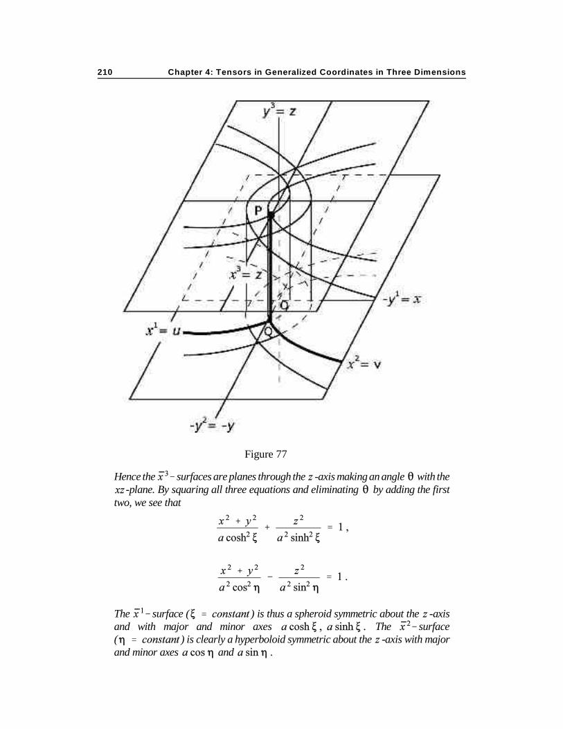
Figure 77
Hence the surfaces are planes through the -axis making an angle with the-plane. By squaring all three equations and eliminating by adding the first
two, we see that
The surface ( ) is thus a spheroid symmetric about the -axisand with major and minor axes The surface( ) is clearly a hyperboloid symmetric about the -axis with majorand minor axes and
1. Coordinate Curves and Coordinate Surfaces 211
Ex. (1.9) Interpret the ellipsoidal coordinates related to Cartesiancoordinates by the transformations
Ans. From the first equation we have
The second and third equations give
Adding the three equations gives
Expanding the numerator of the right hand side, we find that the terms in and drop out and that the remaining terms are identically equal to the denominator.Hence

Chapter 4: Tensors in Generalized Coordinates in Three Dimensions212
Therefore the surface ( ) is an ellipsoid with axes
and In similar fashion, we can show that the
surface ( ) is
a hyperboloid of one sheet with axis the -axis. Finally, the surface( ) has the equation
a hyperboloid of two sheets which open respectively to the positive and negative-axes. In general, the surface is the quadric whose equation is (see Fig. 78).
Figure 78

1. Coordinate Curves and Coordinate Surfaces 213
Ex. (1.10) Show that the line element in a cylindrical coordinate system is
Ex. (1.11) (a) Show that the line element for the spherical coordinate system
of Fig. 71 is
(b) Determine the Christoffel symbols in this coordinate system.
Ans. Those which are not zero are
Ex. (1.12) (a) Show that the line element for the hyperbolic cylindricalcoordinates is
(b) Determine the Christoffel symbols in this system.
Ans.
Ex. (1.13) Show that the fundamental tensor in paraboloidal coordinates is
Chapter 4: Tensors in Generalized Coordinates in Three Dimensions214
Ex. (1.14) Show that the fundamental tensor in elliptical cylindricalcoordinates is
Ex. (1.15) Show that the fundamental tensor in spheroidal coordinates is
Ex. (1.16) Show that in ellipsoidal coordinates the line element is
2. Space Curves
Consider any continuous curve C with a continuous tangent. Let and be the coordinates of nearby points on the curve. The distance along the
curve between the points is the differential of arc length
Therefore the vector
(2.1)
is a unit vector along the curve at the point . It is the unit tangent to the curve at thatpoint.
Since is a unit vector,
Taking the intrinsic derivative of both sides with respect to the arc length gives

2. Space Curves 215
If we define to be the magnitude of and to be a unit vector in thedirection of , i.e. , if
(2.2)
then it is clear from the preceding equation that
Evidently is orthogonal to . We therefore call the principal normal to thecurve C. The invariant is the curvature of C. Thus far our results do not differ fromthose obtained in two dimensions.
Let us now form the intrinsic derivative of the preceding equation. It is
Using equation (2.2), this becomes
Hence
(2.3)
Therefore is orthogonal to the unit vector defined by
(2.4)
On the other hand, since
it follows that
Therefore is orthogonal to as well as to . Hence it is also orthogonalto . The vectors and thus form a mutually orthogonal triad. The senseof is so chosen that this triad is right-handed in the order this requiresthat
(2.5)
The sign of is chosen in equation (2.4) to make this so. The quantity is called thetorsion of the curve, the vector is the curve’s binormal.

Chapter 4: Tensors in Generalized Coordinates in Three Dimensions216
Figure 79
Equations (2.2) and (2.4) express the intrinsic derivatives of two of the triad in terms of the others. This prompts the thought that perhaps it should be
possible to express the third in a similar manner. It is easy to show that this is the case.
First, since forms an orthogonal triad of unit vectors, we may adopt it as abasis system. Then any other vector may be expressed as a linear combination of them;in particular, we may take
where and are the invariants
The value follows at once from the fact that is a unit vector. To find the value
of , we use the fact that
implying that
because of the orthogonality of and
2. Space Curves 217
In similar fashion, we find by starting from the relation
implying that
because is a unit vector and is orthogonal to .
If we use the values of and thus found and express the result along withequations (2.2) and (2.4) in symmetric fashion, we have the Frenet formulae
(2.6)
for a curve in space. In descriptive terms, the quantity measures “how curved” thecurve is and the quantity measures “how twisted” the curve is.
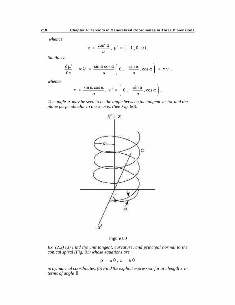
Ex. (2.1) Find the tangent, principal normal, binormal, curvature and torsion tothe regular circular helix whose parametric equations are
in cylindrical coordinates.
Ans. We have first that the unit tangent vector is
Then, since the only Christoffel symbols which do not vanish are
we have
Chapter 4: Tensors in Generalized Coordinates in Three Dimensions218
Figure 80
whence
Similarly,
whence
The angle may be seen to be the angle between the tangent vector and theplane perpendicular to the -axis. (See Fig. 80).
Ex. (2.2) (a) Find the unit tangent, curvature, and principal normal to theconical spiral (Fig. 81) whose equations are
in cylindrical coordinates. (b) Find the explicit expression for arc length interms of angle

2. Space Curves 219
Figure 81
Ans. where
The foregoing algebraic derivation of the Frenet formulae and of thequantities associated with a curve — tangent, normal, binormal, curvature and torsion— may be buttressed by a parallel geometric discussion. To begin with, we define theunit tangent to a smooth curve, whether a plane curve or not, as the unit vector havingthe limiting position of the secant at a point when approaches . We may inthis way define the tangent at all regular points of a curve.
Let us now consider the tangents at neighboring points and . Let the tangent define a parallel vector field, i. e., one satisfying
Chapter 4: Tensors in Generalized Coordinates in Three Dimensions220
The element of this parallel vector field at may be used to determine the differencebetween and at . In the limit as approaches , the direction andmagnitude of as is defined. Since is a parallel vector field,and since as is the limit of the ratio of the difference of and
it can have no part parallel to must therefore lie in the plane normalto This is the normal plane. The normal in the direction of lies in thenormal plane. Perpendicular to , through , is the rectifying plane.
We may apply the procedure once more. Consider the normal at . Let itdefine a parallel vector field along the curve. The element of this vector field at maybe subtracted from and the ratio
formed. Its limit as approaches is It must be perpendicular to and,since is everywhere perpendicular to , it must be perpendicular to also. In thisway, we generate the triad . Clearly, must lie in the rectifying plane. It isorthogonal to the plane of and the osculating plane.
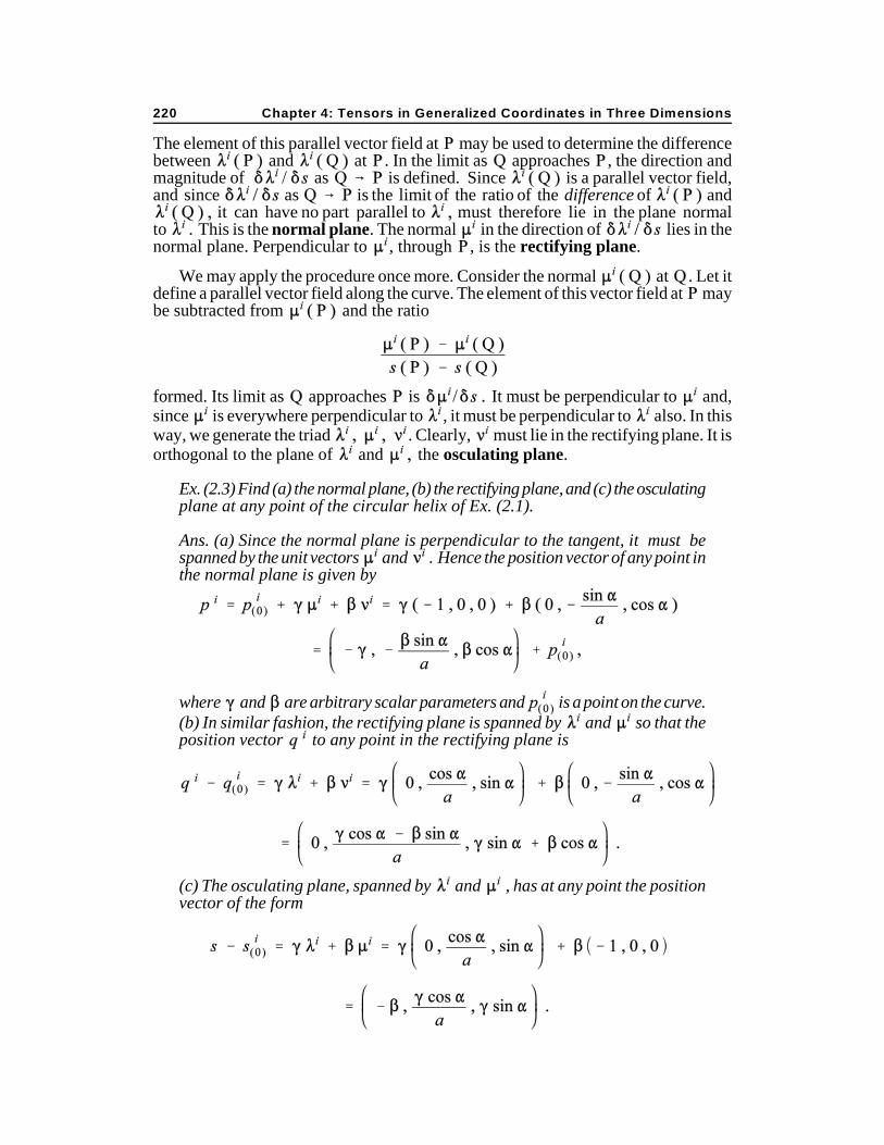
Ex. (2.3) Find (a) the normal plane, (b) the rectifying plane, and (c) the osculatingplane at any point of the circular helix of Ex. (2.1).
Ans. (a) Since the normal plane is perpendicular to the tangent, it must bespanned by the unit vectors and Hence the position vector of any point inthe normal plane is given by
where and are arbitrary scalar parameters and is a point on the curve.(b) In similar fashion, the rectifying plane is spanned by and so that theposition vector to any point in the rectifying plane is
(c) The osculating plane, spanned by and , has at any point the positionvector of the form

2. Space Curves 221
From the Frenet formulae we can deduce very simply certain results ofconsiderable interest. Thus, consider a curve for which i.e., a curve of zerocurvature. Along such a curve
This is identical with the equation for a geodesic in two dimensions. We may thereforedefine a geodesic as a curve whose curvature is zero. (As in two dimensions, we mightalso define a geodesic as a curve of minimum length between two given points. Thedevelopment is identical and the results are the same.)
From the Frenet formulae, we see further that when the curve is a geodesic, i. e. ,when the two remaining equations become
(2.7)
It appears that and are now wholly independent of . This is not true, however,for
with a similar expression for the explicit dependence upon is here evident.However, the vectors and no longer have any necessary relation to other thanorthogonality; in other words, at any point of the curve, we may choose to be anyunit vector orthogonal to the unit tangent. At the same time, equations (2.7) will besatisfied for any if only and are mutually orthogonal. We may show this bymultiplying the first by , the second by , and adding; the result is
Hence
or along the geodesic, where is the angle between and . In particular, if the angle is the vectors and are orthogonal toeach other as well as to . We take this to be the case in order to satisfy equation (2.5).
Let us now look upon equation (2.7) as defining . We choose and as anymutually orthogonal unit vectors which are both orthogonal to . The components of and may be any functions of consistent with these conditions. Then from either ofequations (2.7) we may define a which will satisfy the other equation. The simplestpossible choice of is, of course, In that case, the curve has no torsion andboth normal and binormal are parallel vector fields along the geodesic. It is apparent,however, that a curve of zero curvature may have whatever torsion one chooses to giveit; in this sense, the torsion of a geodesic is indefinite.

Chapter 4: Tensors in Generalized Coordinates in Three Dimensions222
It is of further interest to note the special case of a curve for which In this event, the binormal is a parallel vector field along the curve though the curveis in general not a geodesic. The Frenet formulae then reduce to*
It is clear that we can apply the argument previously given for and to show thatthese equations are satisfied whenever and are orthogonal, as they must be by thedefinition of The curve is then a plane curve.
Ex. (2.4) In three-dimensional Euclidean space, geodesics are straight lines.Without loss of generality, therefore, one may choose the -axis of a Cartesiancoordinate system to represent a geodesic. Along it, , andthe unit tangent is Since we may choose the principalnormal arbitrarily, then require only that the binormal be orthogonal toboth and . (a) If is chosen to be
(a corkscrew field), what is the binormal ? (b) What is the torsion ? (c) Whatform have and when we impose the condition Ans.
Ex. (2.5) In a spherical coordinate system (see Ex. 1.11)), the parametricrepresentation of a curve is
in terms of a parameter and constant Determine (a) the unittangent, (b) the principal normal, (c) the curvature, (d) the torsion, (e) thebinormal. (f) Is the curve a plane curve? (g) Identify the curve.
Ans.
It would appear at first glance that when the Frenet formulae reduce to those for a surface, not*
necessarily a plane. It must be remembered, however, that the intrinsic derivatives have been formed byemploying Christoffel symbols for three dimensions, not two. This distinction is essential.
2. Space Curves 223
Figure 82
Yes. The curve is an exponential spiral lying in the plane tilted at anangle to the -plane and passing through the -axis.
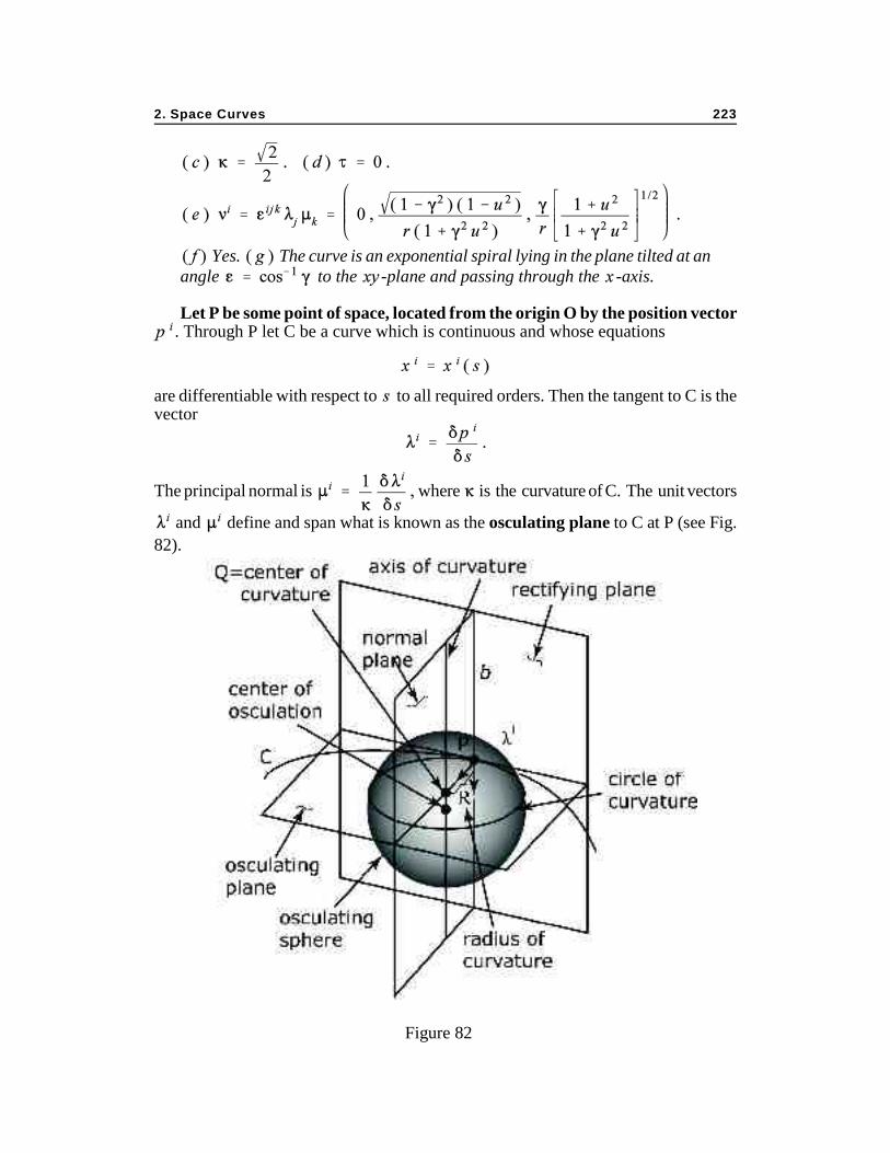
Let P be some point of space, located from the origin O by the position vector
. Through P let C be a curve which is continuous and whose equations
are differentiable with respect to to all required orders. Then the tangent to C is thevector
The principal normal is where is the curvature of C. The unit vectors
and define and span what is known as the osculating plane to C at P (see Fig.
82).

Chapter 4: Tensors in Generalized Coordinates in Three Dimensions224
Consider the straight line L through P in the direction of . Its equation will be
where is the parameter of the line. Let us pick a point such as Q on L, and draw in theosculating plane about Q a circle whose radius is . This circle will obviously passthrough P, as the manner of construction requires it should. Therefore the tangent to thecircle is also a tangent to the curve C. In general, as P moves along the curve E, the pointQ would also be displaced in space. We may ask, therefore, if there is some point Qwhich is stationary with respect to the displacement of P along C. In this case,
would be stationary, having a contact of the third order. Differentiating the previousexpression with respect to gives first
where we have set This simply expresses the fact that and areorthogonal. In order that the circle with center at Q have a contact of the third order atP, we must differentiate once more the expression for giving
Thus the point Q at distance from P in the direction of is called the center
of curvature of the curve C at point P. The quantity is the radius of curvature ofthe curve at P.
Let us consider a further generalization. Suppose that is
where is an undetermined parameter. If taken as a curve parameter, will evidentlygenerate the straight line through Q in the direction of — i. e. ,perpendicular to the osculating plane. This straight line is called the axis of curvatureof the curve C at P.
Now
is the radius of a circle through P with center on the axis of curvature. As P advancesalong the curve C,

2. Space Curves 225
Hence
For a contact of the fourth order, the last expression must vanish. This requires that have the value
(2.8)
Hence the point
is the center of the osculating sphere, having a contact of the fourth order with thecurve C at P. It is the sphere which best fits the curve at P. Its intersection with the
osculating plane is the osculating circle. Since
(2.9)
(2.10)
In summary, we may say that the foregoing development shows how any curve Cmay be characterized at any point by its tangent , normal , binormal , and twoinvariants — the curvature and torsion . These quantities are intimately related bythe Frenet formulae. It is reasonable to suppose, conversely, that any curve may becharacterized in its essentials by its curvature and torsion together with theorientation of the triad and at some point. This proposition may, in fact, begiven a rigorous proof.

Chapter 4: Tensors in Generalized Coordinates in Three Dimensions226
Ex. (2.6) A loxodrome is a curve on the surface of a sphere which at every point makesa fixed angle with the meridian of longitude through the point. Thus its equation is
in spherical coordinates. (Note that when we require that Find (a)the unit tangent; (b) the normal; (c) the binormal; (d) the curvature; (e) the torsion. (Hint:use Ex. (1.11).)
Ans.
Ex. (2.7) For the helix of Ex. (2.1), (a) locate the center of curvature of any point on thecurve; (b) determine the equation of the axis of curvature; (c) find the center of theosculating sphere; and (d) find the radius of the osculating sphere.
Ans. (a) Since the position vector is at any point we have
the axis of curvature associated with any point of the helix is the line defined by the vector
where is the curve parameter; (c) the center of the osculating sphere is at the point
(d) the radius of the osculating sphere is
but since this is

2. Space Curves 227
Ex. (2.8) For the loxodrome of Ex. (2.6), (a) locate the center of curvature, (b) findthe center of the osculating sphere, and (c) determine the radius of the osculatingsphere.
Ans. (a) Since the position vector of any point on the curve is we have
(b) i. e. , the center of the osculating sphere is at the center ofthe sphere on which the loxodrome lies.
(c)
Ex. (2.9) (a) Show that for the loxodrome of Ex. (2.6),
where a prime denotes differentiation with respect to arc length. (b) Show that thisrelation is true for all curves which lie on a sphere. (Hint: as with the loxodrome,the radius of the osculating sphere is the radius of the sphere, hence a constant.Therefore, the derivative
Ex. (2.10) Find the equation of the geodesic when the square of the line elementis given in spherical coordinates as
being the co-latitude on the unit sphere about the origin and the longitude.
Ans. The geodesic equations are

Chapter 4: Tensors in Generalized Coordinates in Three Dimensions228
Here dots denote differentiation with respect to . We may solve these equationsmost simply by noting that
is the square of the line element upon the unit sphere, whose geodesics have beendetermined in Ex. (2.7.10). The line element is now given in three dimensions as
for which the geodesic equations (see Ex. (2.7.9)) are
A first integral of the last equation is
Therefore
Furthermore, the third of the geodesic equations has the integral
Using these integrals in the second geodesic equation gives
and since
this may finally be given the form
which is identical with the first of equations (2.7.33), and therefore has the samesolution. At the same time, the preceding equation is of the same form as equation(2.7.34). Hence by combining the solutions of Exs. (2.7.9-10), we get as theequation of the geodesic
3. The Dynamics of a Particle 229
Ex. (2.11) Find the equation of the geodesic when the square of the line elementis given in geodesic polar coordinates as:
3. The Dynamics of a Particle
Aparticle is conveniently defined as a mass point. This means that it haslocation, as specified by a set of coordinates , and mass, as specified by an
invariant . A particle in motion will have coordinates which are a function of theinvariant time . Hence
is the particle’s velocity vector. Its momentum vector is
Newton’s Second Law of Motion states that the force upon the particle is
measured by the product of its mass and acceleration; that is,
(3.1)
in an inertial system.*
An inertial system is a frame of reference in which any particle continues in a state of rest or of uniform*
straight line motion unless acted upon by an external force. Newton’s First Law thus defines inertialsystems and it is only in such systems that Newton’s Second and Third Laws are valid.
Chapter 4: Tensors in Generalized Coordinates in Three Dimensions230
Ex. (3.1) What are the components of the force vector in spherical coordinates?(Hint: make use of the results of Ex. (1.11).)
Ans.
where a dot denotes differentiation with respect to time. An important invariant defined by the mass and velocity of a particle is its
kinetic energy
(3.2)
One of the features of the kinetic energy which makes it particularly useful is the factthat from it the force vector may be calculated with comparative ease. Thus consider theequation
where dots denote differentiation with respect to . Then

3. The Dynamics of a Particle 231
From equation (3.2) it is clear that this may be written as
(3.3)
Thus the covariant force vector is obtainable directly in any coordinate system from thekinetic energy . The expression on the right hand side of equation (3.3) is sometimesreferred to as the Lagrangian or Eulerian derivative of .
Ex. (3.2) Find (a) the kinetic energy of a particle and (b) the components of itsLagrangian derivatives in spherical coordinates. (c) From (b), determine thecontravariant components of the Lagrangian derivative.
Ans.
Same as Ex. (3.1).
We can now show quite generally that the Lagrangian derivative of anyinvariant function is a covariant vector. We do so by showing that itsatisfies the covariant vector transformation. To this end, let us consider the two terms
of the Lagrangian derivative separately. First, we note that
and that and in the left member can be expressed in terms of and as
whence it follows that
Therefore the partial derivative of with respect to is
(3.4)
which by the preceding relations becomes
(3.5)

Chapter 4: Tensors in Generalized Coordinates in Three Dimensions232
showing that is a covariant vector. (When it is clear from anyconcrete example or from equation (3.2) that this vector is the covariant momentumvector.)
The first term of the Lagrangian derivative is now
This term is clearly not by itself a vector. At the same time, the second term of theLagrangian derivative is
By subtracting this last equation from the last of the previous equations, we see that
From this it is evident that the Lagrangian derivative of any invariant function of thecoordinates and their derivatives is a covariant vector. In the special case when we see that the vector is the covariant force vector. The Lagrangian derivative of otherinvariant functions could be identified similarly when known in explicit coordinatesystems.
The force defined in equation (3.1) is distinguished as the kinematic form. It ispurely a definition, given solely in terms of the observed motion of the particle. Onedoes not have an equation of motion until the kinematically defined force is equated toa force defined dynamically by the universe in which the particle is set. For example,the particle may be set in a universe with one other mass, to which it is attractedgravitationally ; the dynamical force is then the inverse square force of gravity. Otheruniverses will clearly define other dynamical forces.
Of most interest in the dynamics of particles are those dynamical forces which maybe expressed as the Lagrangian derivatives of an invariant function known as thepotential function, . For these, we have that
(3.6)
3. The Dynamics of a Particle 233
Note that if is independent of the covariant force vector is given simply by thepartial derivative of with respect to This latter is in this case called thegradient of . It is important to realize that in general this is a vector only when is independent of Velocity dependent potential functions are the exception,however, so that it is often stated somewhat loosely that the force may be derived as thegradient of the potential.
Ex. (3.3) Given the gravitational potential function
in spherical coordinates, where is the constant of gravitation and and are the masses of the two attracting bodies, what are the components of theLagrangian derivatives of ?
Ans.
Ex. (3.4) Consider the coordinate system related to spherical coordinates by thesub-tensor transformation
(a) Find the covariant components of the force vector in this coordinate system.(Hint: transform the equations obtained in Ex. (3.2)). (b) Express the gravitationalpotential (see Ex. (3.3)) in these coordinates and find its Lagrangian derivatives.
Ans.
Ex. (3.5) Find the Lagrangian derivatives of the velocity-dependent gravitationalpotential
expressed in the coordinate system of Ex. (3.4) , where is a universal constant.(This potential function may be seen to be an invariant function if we write it as

Chapter 4: Tensors in Generalized Coordinates in Three Dimensions234
where is the position vector, the velocity vector, and thecovariant basis vector along the curve in a spherical coordinate system.Under the transformation of Ex. (3.4) it takes the form given above.)
This classical potential function is of particular interest because it predictscorrectly the advance of the perihelion of Mercury (see Appendix 4.1). It wasproposed in 1898 by Paul Gerber (Zs. f. Math. u. Phys., v. xliii, pp. 93-104). Heinterprets the constant as the velocity of gravitation, which is found to be thesame as the velocity of light.
Ans.
We may now equate the kinematic and dynamical forces defined respectivelyby equations (3.3) and (3.6). The resultant equation of motion is
Let us define the Lagrangian function to be
(3.7)
From the preceding equation it therefore follows that the equations of motion of aparticle are
(3.8)
They are called Lagrange’s equations.
Ex. (3.6) Find Lagrange’s equations, in a spherical coordinate system, for theharmonic oscillator.
Ans. Since the Lagrangian function is
Hence

3. The Dynamics of a Particle 235
Figure 83
Ex. (3.7) Determine Lagrange’s equations for a simple pendulum. Take it to be aspherical bob of mass at the end of a rigid weightless bar of length . Use thedisplacement angle as variable (see Fig. 83).
Ans. Since
Hence we get
Ex. (3.8) Suppose that the pendulum of Ex. (3.7) is elastic rather than rigid. Thenwhat do Lagrange’s equations become?
Ans. Take to be the equilibrium length of the rod. Then extension or
compression of the rod gives it a potential energy where is the elastic constant. Therefore
Hence
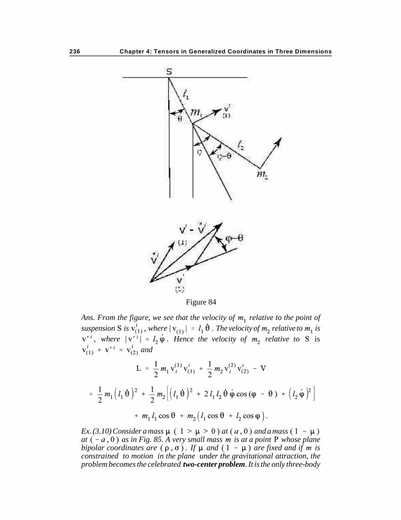
Ex. (3.9) Consider the compound pendulum (Fig. 84). It consists of masses and (subscripts here are not tensor indices) at the ends of rigid weightlessrods of respective lengths and asshown. What is the Lagrangian function of this system?
Chapter 4: Tensors in Generalized Coordinates in Three Dimensions236
Figure 84
Ans. From the figure, we see that the velocity of relative to the point of
suspension is where The velocity of relative to is
where Hence the velocity of relative to is
and
Ex. (3.10) Consider a mass at and a mass at as in Fig. 85. A very small mass is at a point whose planebipolar coordinates are If and are fixed and if isconstrained to motion in the plane under the gravitational attraction, theproblem becomes the celebrated two-center problem. It is the only three-body

3. The Dynamics of a Particle 237
Figure 85
problem of celestial mechanics whose general solution can be expressed interms of quadratures. Derive and solve Lagrange’s equations for the smallmass in elliptical coordinates.
Ans. See Appendix (4.2).
Ex. (3.11) Show that the kinetic energy of a rigid body is
where is the moment of inertia tensor, the angular velocity, the totalmass, and the velocity of the center of gravity.
Ex. (3.12) A particle of mass is constrained by gravity to movefrictionlessly over the outer surface of a hemisphere. Find the equations ofmotion.
Ans. Take the center of the sphere of radius to be the origin of a sphericalcoordinate system. Then
Then Lagrange’s equations become
(Note that leads to results similar to those of Ex. (3.7).)

Chapter 4: Tensors in Generalized Coordinates in Three Dimensions238
The importance and utility of Lagrange’s equations can be grasped only veryimperfectly from the few illustrations here presented. In Ex. (3.6) we see how they giveNewton’s equations 11 of motion in a very straightforward and economical way. InEx. (3.7), we consider a standard problem which, however, has relatively simple yetinteresting generalizations in Exs. (3.8) and (3.9). Each new variable required definesanother degree of freedom. Clearly, the number of degrees of freedom may beincreased indefinitely, independent of the number of dimensions of the space. In Ex.(3.10) we have an illustration of the value of certain specialized coordinate systems,without the use of which the solution of some problems would be very difficult or evenimpossible. Lagrange’s equations apply also to rigid bodies, as may be seen in Ex.(3.11); in fact, they can be shown to hold for continuous media as well. And finally,problems which include constraints, as in Ex. (3.12), may be readily handled byLagrange’s equations.
Lagrange’s equations are not only convenient as equations of motion but convenientalso for the close relation they bear to other forms of the equations of motion.*
To consider these, let us first define the generalized momentum; it is
(3.9)
If the potential is independent of this is the same as the ordinary momentumpreviously defined as
Otherwise it is more general, whence the designation as “generalized momentum”.(It is clearly a covariant vector, obtained by setting ) Now from Lagrange’sequations we have that
(3.10)
We now look upon equation (3.9) as the definition of a new variable We write it as
Assuming that this is a reversible transformation, we can solve it for as
(3.11)
In particular, they are derived from a Legendre transformation, by which a function becomes* a function where and such that In our application of the Legendretransformation, the function is where stands for and for Then
becomes , and, as is shown in what follows, is the Hamiltonian function

3. The Dynamics of a Particle 239
Note that this is not a simple point transformation of coordinates, such that the values of determine the values of It is a more general transformation which determines
from and or from and
Next, from the vectors and the invariant we form anew invariant
(3.12)
It is called the Hamiltonian function. Differentiating partially with respect to weget
(3.13)
Differentiating partially with respect to next, we get
(3.14)
according to equations (3.9) and (3.10). From equations (3.13) and (3.14), we thus havein final form Hamilton’s canonical equations
(3.15)
It is interesting to note that is a vector, since generalized velocities in any case areso. Therefore is likewise a vector. On the other hand, though (as we haveshown) is a covariant vector, is in general not a vector except in a rectilinearcoordinate system, where it is identical to However, since
in one coordinate system, it must be zero in all. Hence this quantity is a covariant vectoreven though its separate terms need not be. It is for this reason that the second ofequations (3.15) has been put in this form. In this form, Hamilton’s equations are vectorequations.
Ex. (3.13) Find Hamilton’s equations for the harmonic oscillator in threedimensions.
Ans. From Ex. (3.6), we have
Therefore
Chapter 4: Tensors in Generalized Coordinates in Three Dimensions240
Hence
Ex. (3.14) Find Hamilton’s equations for the simple pendulum.
Ans. From Ex. (3.7) we find that
Ex. (3.15) From Hamilton’s equations, show that
Hence show that when the kinetic energy is a quadratic homogeneousfunction of and the potential energy is independent of , we have
where is the total energy of the system. Such a system is said to beconservative.
Ans. For any system whose Hamiltonian is we have
whence the first result follows.
If this is a quadratic homogeneous function of , then by Gauss’s theoremon homogeneous functions
whence the second result follows if we define the total energy to be the sum ofthe kinetic and potential energies.

4. Geometrical Dynamics 241
4. Geometrical Dynamics
Lagrange’s equations are also closely related to still another form of theequations of motion. We recognize the equations
as identical with the equations to be satisfied by that curve along which the line integral
(4.1)
is an extremum. The quantity is called the action when is the Lagrangian function.Lagrange’s equations therefore require that the motion of a particle be such that itsaction integral is an extremum — in particular, a minimum. Therefore the motion of aparticle is said to obey the Principle of Least Action.
As we have seen (Ex. (3.15)), for a conservative system it is true that so that In this case, the action
integral is
Therefore, if the times and are fixed, and if we consider variations of the path underthis condition, it will be true that
is the condition for an extremum. Now
so that
Therefore the principle of least action for a conservative system requires that
(4.2)
Let us now define a conformal mapping (see Ch. 2, Sec. 8, Eq. (8.5) )
(4.3)
In terms of the new line element, the action integral becomes
Chapter 4: Tensors in Generalized Coordinates in Three Dimensions242
Since
it is clear that the action is stationary when the path length on the map is minimal - i. e.,geodesic. The quantity is called the action line element to distinguish it from thekinematic line element . Thus the geodesics of the action line element map intothe natural trajectories of the kinematic line element, and conversely. This process issometimes referred to as the geometrization of dynamics. It is of considerableimportance in the general theory of relativity.
Ex. (4.1) Show that
where is the Christoffel symbol derived from the kinematic line element
and is that derived from the action line element.
Ex. (4.2) Show that Lagrange’s equations in the kinematic metric become thegeodesic equations in the action metric.
Ans. We write Lagrange’s equations in the contravariant form
Substituting for from Ex. (4.1), we get
However, since
the right hand side vanishes. Hence
5. Green’s and Stokes’ Theorems 243
By Ch. 2, §4, this is equivalent to
where
Ex. (4.3) Is the mapping defined by equation (4.3) geodesic? (Hint: see Ch. 2, Sec.8, Eq. (8.11).) Ans. No. (Caution: note that equation (8.11) must be modified forthree-dimensional mappings. In this case
In dimensions,
5. Green’s and Stokes’ Theorems
We have seen that vectors of special interest may be generated bydifferentiating invariants; the Lagrangian derivative is an example. A case of
particular interest arises when an invariant is a function of the coordinates only.In that case, the vector
to which, apart from sign, the Lagrangian reduces in this instance, is called the gradientof . Examples of invariants whose gradients arise in physical applications aretemperature, gravitational potential, chemical concentration, electric charge density, etc.
Gradients also figure frequently in a converse process of generation of invariantsfrom derivatives. For example, consider a vector . From its covariant derivatives we can form the invariant This quantity is called the divergence of the vector .Clearly, the divergence of a covariant vector may also be formed simply by first puttingit in a contravariant form. Thus
(5.1)
so that the final expression is the divergence of . When is the gradient of , thisbecomes
The operator here denoted by is called the Laplacian. It is an important invariantoperator.

Chapter 4: Tensors in Generalized Coordinates in Three Dimensions244
The divergence and Laplacian operators are of such frequent occurrence inmathematical physics that it is convenient to express them in a form most expedient forcalculation in explicit coordinate systems. Consider the divergence of . It is
To find a useful expression for , we first note that
Substituting for its equivalent, this gives
Consider the particular case when Then
Clearly, the only terms on the right hand side which survive the summation over arethe ones in which in the first, in the second, and in the third.Hence (compare with Ex. (3.10) of Ch. 2)
(5.2)
We may now use this identity in the expression for the divergence of . The result is
(5.3)
Because of its simplicity, this is the most expeditious formula for the divergence of avector .
If we now combine the results of equations (5.1) and (5.3), we find for the Laplacianof the result

5. Green’s and Stokes’ Theorems 245
In Cartesian coordinates, the Laplacian takes the familiar form
Ex. (5.1) Find the Laplacian of a function in (a) cylindrical coordinates, (b)spherical coordinates, and (c) parabolic cylindrical coordinates. (Hint: see Exs.(1.10, 1.11, 1.12).)
Ans.
Ex. (5.2) Find the divergence of a vector in (a) cylindrical coordinates,(b) spherical coordinates, and (c) parabolic cylindrical coordinates.
Ans.
Perhaps the most important use of the divergence is in the statement ofGreen’s theorem, which permits the transformation of surface integrals into volumeintegrals or vice versa. We state the theorem first in Cartesian coordinates, then translateit into generalized coordinates. The theorem says that if is a closed surface boundinga volume (Fig. 86), and if and are three continuous functions havingpartial derivatives of the first order throughout and over , then
where and are the direction cosines of the outward normal of . Thistheorem, to be found in any text on advanced calculus, may be proven readily byintegrating partially along lines parallel to the coordinate axes.

Chapter 4: Tensors in Generalized Coordinates in Three Dimensions246
Figure 86
Let us now identify the integrand on the left hand side. The direction cosines aresimply the covariant components of the unit normal . The functions and may be taken as the components of a contravariant vector . Hence the integrand on theleft is nothing but , an invariant.
Now let us write the integrand in the right hand side as
Remembering that in Cartesian coordinates
we see that this integrand is the divergence of , an invariant.
By identifying the integrands in Green’s theorem as invariants, we are now able toexpress the theorem in any system of coordinates. It is contained simply in the equation
(5.5)
The quantity is called the flux of across the surface . This terminologyaccords with the interpretation of when represents the rate of flow of matter,momentum, energy or similar quantity.
5. Green’s and Stokes’ Theorems 247
To interpret the divergence , let us consider a unit volume . If there is a positivenet flux from , as measured by the left hand side of equation (5.5), this means thatmore of the quantity whose flow is represented by has flowed out of than flowedinto . There has thus been a creation of this quantity within . But the right hand sideof equation (5.5) is the integral of over the unit volume . Hence the divergence of must represent the rate at which the quantity is created per unit volume. Therefore, if
, the quantity is said to have a source within ; if , the quantity is saidto have as sink within . If the quantity is conserved.
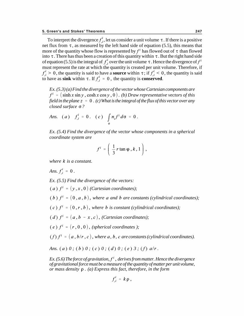
Ex. (5.3) (a) Find the divergence of the vector whose Cartesian components are (b) Draw representative vectors of this
field in the plane (c) What is the integral of the flux of this vector over anyclosed surface ?
Ans.
Ex. (5.4) Find the divergence of the vector whose components in a sphericalcoordinate system are
where is a constant.
Ans.
Ex. (5.5) Find the divergence of the vectors:
(Cartesian coordinates);
where and are constants (cylindrical coordinates);
where is constant (cylindrical coordinates);
(Cartesian coordinates);
(spherical coordinates );
where , , are constants (cylindrical coordinates).
Ans. 0 ; 0 ; 0 ; 0 ; 3 ;
Ex. (5.6) The force of gravitation, derives from matter. Hence the divergenceof gravitational force must be a measure of the quantity of matter per unit volume,or mass density (a) Express this fact, therefore, in the form

Chapter 4: Tensors in Generalized Coordinates in Three Dimensions248
which is satisfied by the gravitational force, where is constant. (b) Show that thegravitational potential thus satisfies the equation
The customary form for the constant is where is the constant ofgravitation. This equation is known as Poisson’s equation.
In addition to the examples thus far given, yet another vector of particularinterest may be generated from the derivatives of a given vector. It is the curl of defined to be
(5.6)
We may express it quite simply just by writing out its components. Thus
Consider the first component. It is
A similar computation for the remaining two components shows that
(5.7)
This is usually the most convenient form in which to calculate the curl of any covariantvector. The curl of any contravariant vector is to be found by lowering the index first,then proceeding as above.
The curl of a vector figures in the statement of another integral theorem, Stokes’theorem. Again, we state it first in Cartesian coordinates and from this derive astatement in any coordinate system. The theorem says that if is a portion of asurface enclosed by a contour (see Fig. 87) and if and are threecontinuous functions having partial derivatives of the first order over , then
where and are the direction cosines of the normal to and the line integralon the left is taken entirely around . Proof of this theorem, like that of Green’stheorem, will be found in any text on advanced calculus.

5. Green’s and Stokes’ Theorems 249
Figure 87
Again we proceed by identifying the integrands of the preceding equation asinvariants. If then the integrand on the left hand side is the invariant
Reference to equation (5.7), together with the fact that in Cartesian coordinates allows us to write the integrand on the right side as
Therefore the statement of Stokes’ Theorem may be written in the generalized form
(5.8)
The integral on the left is sometimes called the circulation of about the curve .
Note that if is the gradient of an invariant , then the curl of is zero, for

Chapter 4: Tensors in Generalized Coordinates in Three Dimensions250
and by equation (5.7)
Conversely, when the curl of a vector is everywhere zero, the vector must be expressibleas the gradient of some invariant . For then, by Stokes’ Theorem,
for any curve . This means that the integrand is a perfect differential; that is,
whence it follows by partial differentiation that
Such a vector is called irrotational.
Ex. (5.7) Find the curl of the vectors of Ex. (5.5).
Ans. ( 0 , 0 , 0 ); ( 0 , 0 , 2a ); ( 0 , 0, 3r );
( 0 , 0 , - 1 ); ( 0 , 0 , 0 ); ( 0 , 0 , b / r ).
Ex. (5.8) If
Ans.
Ex. (5.9) Show that the divergence of of Ex. (5.8) vanishes identically. Hence
show that the divergence of the curl of any vector is zero.

5. Green’s and Stokes’ Theorems 251
We are now able to derive a result of great interest and usefulness. To do so,we need to make use of the fact* that the components of any continuous anddifferentiable vector field may be expressed uniquely as the Laplacian of thecomponents of a suitably constructed vector field ; that is, we may take
Now from Ex. (5.9),
Hence if we set we see that
(5.9)
The scalar and vector potentials in terms of which is expressed are not unique. Wehave thus shown that a suitably continuous and differentiable vector may beexpressed as the sum of the gradient of some invariant and the curl of some vector. Theinvariant is the scalar potential and the vector is the vector potential.
We see that an irrotational vector is one for which the second term on the right handside of equation (5.9) vanishes. A non-zero vector for which the first term on theright hand side of equation vanishes is called a solenoidal vector. By Ex. (5.9), thedivergence of a solenoidal vector is zero. This result is the counterpart of the fact thatthe curl of an irrotational vector is zero.
Ex. (5.10) Show that a vector of the form is solenoidal, where and are invariants. (Hint: what is the divergence of ?)
Ex. (5.11) Show that the vector potential for the vector of Ex. (5.10) may betaken to be
Ex. (5.12) Show that if a volume enclosed by a surface contains a surface on which the vector has a jump discontinuity, then
where the parenthesized subscripts (1) and (2) denote the two sides of the surface.
Ex. (5.13) Show that the vector potential is indeterminate to the extent of anarbitrary irrotational vector.
We will take this result of the theory of functions of real variables without proof. It is a familiar*
theorem from potential theory. A fuller discussion of it may be found in Phillips’ “Vector Analysis”(Wiley, 1933), Ch. VIII, for example.

Chapter 4: Tensors in Generalized Coordinates in Three Dimensions252
Figure 88
6. The Equations of Motion of a Continuous Medium
The laws of mechanics of continua are fundamentally the same as those of themechanics of a particle. For continua, however, the particle becomes a small mass
element, with the difference that the elements are contiguous and may interact at theircommon boundaries.
Consider an element of volume in a continuous medium. If it contains an amountof matter , the matter of the medium is said to have a local density
(6.1)
According to Newton’s second law of motion, the acceleration produced in such anelement will be the result of the action of a force of amount
Such forces may originate either from a force field (gravitational, electrical, magnetic,etc.) or from the application of forces to the boundary surface of the medium which, bytransmission throughout the medium, may be present as internal forces. Field forceexists even in the absence of the medium; internal forces require the presence of themedium.
Suppose that the field produces an acceleration determinable from the nature ofthe field and the medium. Its contribution to the net force acting upon an element of themedium will be

6. The Equations of Motion of a Continuous Medium 253
The internal forces, which provide the remainder of the acceleration, must be consideredin greater detail. To this end, consider a surface element bounding . Across thissurface, the element interacts with adjacent elements. In general, the force per unitarea, which we denote by exerted by an adjacent element on , need not be in thedirection of the normal to ; for example, the motion of one sticky surface acrossanother calls into play such forces as drag, parallel to the surfaces. Geometrically, thismeans that the force at any point, represented by a directed line segment, need not liealong the unit normal to the surface. However, since both force and normal can berepresented as straight line segments issuing from a common point, one may betransformed into the other by a linear transformation which will effect a rotation and achange of scale of the proper amount. In other words, we may be assured that there isa set of quantities such that
(6.2)
The quantities are the components of the stress tensor.
The stress tensor may be simply interpreted. Suppose, for example, that we choosea Cartesian coordinate system and that we select an orientation of the surface element such that the unit normal is parallel to the axis; the components of this unit normalwill then be ( 1 , 0 , 0 ). In this case, therefore, we will have
Evidently, the force per unit area has a component of amount along the unit normalas well as components and in the tangent plane of the surface element. Analogousinterpretations may be given the remaining components of the stress tensor.
We must now somehow combine the effects of the volume and surface forcesthrough the medium. To do this, let be any parallel vector field, for which
Then the projections on of the volume and surface forces of the medium, summedover an arbitrary volume enclosed by an arbitrary surface will be
Expressing in terms of the stress tensor, this becomes
We next transform the surface integral on the right hand side by applying Green’s
theorem,

Chapter 4: Tensors in Generalized Coordinates in Three Dimensions254
since by hypothesis Using this transformation, the equation of motionrequires that
for any parallel vector field or volume . This can be true only if the quantity inparentheses vanishes, i. e., if
(6.3)
This is the equation of motion in a continuous medium.
If, as is ordinarily the case, the material of the medium is conserved, thiscircumstance requires that, by Green’s Theorem, the flux of matter have adivergence which equals the rate of accumulation (positive or negative) of the matter.Thus, within a volume , the total amount of matter is changing at a rate of
(The negative sign arises since is the outward normal, whence a positive flux willreduce the amount of matter within .) Hence
for any volume . Therefore it must be true that
(6.4)
This is the equation of continuity for the medium.
Ex. (6.1) Show that the equation of continuity may be written also in the form
Thus show that an incompressible fluid ( ) has constant density.
Ex. (6.2) Write out the equation of continuity in (a) Cartesian coordinates,(b) spherical coordinates, (c) cylindrical coordinates.

7. Isotropic and Viscous Media 255
Ans.
7. Isotropic and Viscous Media
Consider the case when the stress is isotropic. According to our previousdefinition of isotropy, this requires that
(7.1)
where is an invariant. The meaning of may be inferred from the fact that
whence
In other words, the force per unit area, the same in all directions, has a magnitudewhose value is . Therefore is called the pressure within the medium. We may alsosee that from equation (7.1) the value of is given by
(7.2) By this relation, pressure may be defined even in anisotropic media.
A fluid in which the stress is isotropic is called a perfect fluid. Combiningequations (6.3) and (7.1), we obtain
(7.3)
as the equation of motion of a perfect fluid.
Now suppose that the fluid is not perfect; it is then said to be viscous. For a viscousfluid we may therefore write
(7.4) or
The tensor is called the viscosity tensor. Clearly, the viscosity measures the extentto which the stress differs from a pure pressure. Alternatively, a fluid which is notperfect must support a strain. Now by equations (3.8.3) and (3.8.4) a strain is describedby a rate of strain tensor
Chapter 4: Tensors in Generalized Coordinates in Three Dimensions256
(7.5)
where, from equation (3.8.2), Therefore
(7.6)
is called the velocity strain tensor. It is clearly symmetric in and .
Any relation between viscosity and strain must be such that the viscosity vanisheswith the strain. This condition can be secured most simply by requiring the viscositytensor to be a linear function of the rate of strain Thus, we get
(7.7)
where is a tensor of fourth order, symmetric in and . The components of are called the viscosity coefficients. With these, equation (6.3) takes the form
(7.8)
as the equation of motion of a viscous fluid. If the field is homogeneous, then willconstitute a parallel tensor field when both and do so. The condition thereforeis
A circumstance of special interest is the case of isotropic viscosity. By our definition
of isotropy, this means that the coefficient of viscosity tensor must be expressible interms of the fundamental tensors and together with whatever invariants may beneeded. Remembering that is symmetric in and , we see that the most generalisotropic coefficient of viscosity tensor symmetric in and will have the form
where and are invariants.* From equation (7.7) we thus have for the isotropicviscosity tensor
(7.9)
Note that is now also symmetric in and .*
7. Isotropic and Viscous Media 257
The equation of motion of an isotropic viscous fluid is therefore
(7.10)
This equation may be simplified somewhat. By our definition of pressure, it is truethat
whence
Therefore
for arbitrary . This can be true only if
Consequently, the invariants and must satisfy the condition that
The equation (7.10) then becomes
(7.11)
When is constant, and when as is true in any flat space, the lastterm on the right hand side may be written as
Therefore equation (7.11) becomes
(7.12)
Ex. (7.1) Consider a star in static equilibrium and in which the force field isderivable from a gravitational potential . Since it is static, the velocity straintensor vanishes. Write down the equation of motion in spherical coordinates forthe case when the potential is spherically symmetric.
Ans.

Chapter 4: Tensors in Generalized Coordinates in Three Dimensions258
Ex. (7.2) Consider a rotating star of non-viscous fluid in which the force fieldis derivable from a combined gravitational and rotational potential
where is a constant angular velocity in a polar coordinate system in which is the axis of rotation. What are the equations of motion?
Ans.
Ex. (7.3) From equations (3.8.3) and (4.7.5) show that at any point in a fluidwe may define a local angular velocity tensor
(7.13)
From this, show that the local angular velocity vector is
(7.14)
This is sometimes also known as the vortex vector or vorticity vector. Thecurves which satisfy the differential equation
are called vortex lines.
Ex. (7.4) From equation (2.14) and our previous definition of solenoidalvectors, we see that the angular velocity vector is solenoidal. Show, therefore,that characterizes an irrotational velocity field, hence derivable froma velocity potential.
8. The Equations of Electromagnetism in Empty Space
It is well known that certain simple processes such as rubbing glass with silkcan be made to alter the conditions of these materials in that they will attract small
light objects such as bits of paper. Bodies whose condition has been so altered are saidto have been electrified.
If a body has been electrified, its electrification may be transferred wholly or in partto other bodies by placing it in contact with them. By so doing, all bodies may thus beclassified as dielectrics (insulators) or conductors according as the electrification ofthem in empty space may be arbitrarily localized or not.

8. The Equations of Electromagnetism in Empty Space 259
The electrification of a body is attributed to the presence of electric charge uponits surface. Simple experiments such as placing charged bodies in one another’s presenceshow that electric charges are of only two kinds, positive and negative. The sameexperiments establish that like charges repel and unlike charges attract.
If an electrically charged body is brought into the presence of a theretoforeunelectrified body, the latter will be found to have acquired a charge distribution on orwithin it. These are called induced charges. It is by this process of induction that glassrubbed with silk is able to attract light objects nearby.
In principle, induction creates a difficulty for the investigation of chargedistributions, for the presence of electric charges can be known only by the forces theyproduce upon other charges (test charges), and the latter modify the distribution of theformer by the addition of induced charges. The perturbation of a charge distribution maybe made arbitrarily small, however, by making the test charge arbitrarily small. Allassertions about charge distributions imply the use of arbitrarily small test charges.
From the complete symmetry of a sphere and the fact that conductors are specificallycharacterized by the fact that electric charges cannot be localized on or in them, weconclude that in otherwise empty space the charge on the surface of a conducting spheremust be distributed uniformly. We may thus define a point charge as the limitapproached by a conducting sphere as its volume approaches zero. Test charges areideally point charges of infinitesimal strength. Charge distributions may be idealized asdistributions of point charges over surfaces, through volumes, or at isolated points.
Since electric charges on any body give rise to forces on the body when in thepresence of other charged bodies, the displacement of any charge can be effected onlyby the performance of work. The amount of work done in an infinitesimal displacement
of a charge on which forces act will by definition be
(8.1)
It is an experimental fact that in the presence of a static charge distribution, the workdone by a charged body in traversing any closed circuit in empty space is zero. Thisimplies that is the perfect differential of a single-valued function Hence
(8.2)
The quantity is called the electrostatic potential of the given charge distribution.Like other forms of energy, electrostatic potentials of distinct charge distributions areadditive.
Two problems now present themselves: (1) to find the form of the potential function; and (2) to define quantity of charge by prescribing a method of measuring it. Now
it can be shown experimentally that within a closed conducting surface there are noelectric forces due to charges on the surface, for the work done by displacing a chargewithin the conducting surface is found to be independent of the surface charges. Inparticular, if no charges are present within the surface, no electrostatic forces will existin it, no matter what distribution of charges exists on the enclosing surface.

Chapter 4: Tensors in Generalized Coordinates in Three Dimensions260
This result suffices to fix partially the form of the potential function . We note firstthat any charge on the conducting surface will distribute itself in such a way under theaction of its own electrical forces that the net electrical force vanishes everywhere in theinterior of the surface. The fact that the net force of surface charges is everywhere zeroon a small test charge within the closed conducting surface does not mean that the forcebetween it and each charged surface element is zero but only that the sum of the forcesof all such elements together is zero. Since the force exerted by any surface elementupon the test charge is equal and opposite to the force exerted by the test charge uponthe surface element, we may find the total upon the test charge by summing the forceover the conducting surface. This latter force is normal to the surface, else aredistribution of charge would take place. Hence the magnitude of the force at any pointof the surface is where is the unit normal to the surface, and the net forceover the surface is
By Green’s Theorem, this implies that
for any conducting surface bounding the volume . Therefore we must have
(8.3)
Expressing in terms of the potential, this gives
That is, satisfies Laplace’s equation in empty space. In spherical coordinates, withradius , longitude latitude this becomes
(8.4)
Inasmuch as (1) any charge distribution may be constructed from a distribution of pointcharges, (2) the potential functions of distinct charges are additive, and (3) Laplace’sequation is linear in , it will serve to determine the electrostatic potential of all chargedistributions in otherwise empty space if we determine the potential of a single pointcharge. To this end, we continuously deform the surface into a sphere with center atthe origin, taken to be the position of the test charge. The purpose in so doing is torender all surface charges equivalent because of the sphere’s symmetry about its center.Since this process in no way affects the preceding argument, the electrostatic potentialmust still satisfy Laplace’s equation. Hence, by imposing spherical symmetry upon — i.e., by making it independent of and — we find that the potential functionof a point charge must satisfy the equation

8. The Equations of Electromagnetism in Empty Space 261
(8.5)
The arbitrary additive constant is taken to be zero so that will vanish as approaches infinity. The preceding equation expresses Coulomb’s law.
Let us now turn to the problem of measuring the quantity of charge. We wish todefine charge in terms of mechanically measurable quantities. For a point charge, thismay evidently be done by computing the flux of force over any circumscribing surfacenot containing other charges, for since the very presence of the electric charge is knownonly by the force it exerts on other charges and since that force varies as the inversesquare of the distance between point charges, the quantity
is an invariant of the charge, being a proportionality factor dependent upon thechoice of units.
Since the relation between two point charges is entirely reciprocal and since eithermay be used to measure the charge on the other, we must in fact require the flux of forceto be proportional to the charge of each and therefore proportional to both. In otherwords, the product of the charges and is given as
(8.6)
In the rational system of units (or Heaviside-Lorentz units), Electrostatic units are defined when unit charges separated by unitdistance ( ) produce unit force. Therefore
(8.7) .
Electromagnetic units are defined by the relation , whence
(8.8)
Having prescribed a purely mechanical method for measuring electric point charges,and having agreed upon a system of units, let us consider an arbitrary volumedistribution of point charges. The quantity of charge within a surface will be
Chapter 4: Tensors in Generalized Coordinates in Three Dimensions262
if we use as a test body a unit charge At the same time, if point charges aredistributed with density through the volume within , then
By equating the two expressions for and applying Green’s Theorem, it follows that
(8.9)
We have tacitly assumed that the electric point charges are distributed throughotherwise empty space. In this case, represents the force per unit charge, a quantitydefined to be the electric field strength, Equation (8.6) thus becomes
(8.10)
one of the fundamental equations of electromagnetism. Note that essential modificationsof the equations of electrostatics are necessary for charges distributed through materialmedia.
Ex. (8.1) A line of force is defined to be a curve whose unit tangent has thedirection of the electric force vector, hence
Show that the lines of force are orthogonal to the equipotential surfaces.
Static distributions of electric charge are, as such, of little interest, for theirstatic character guarantees that nothing happens to them. On the other hand, charges inmotion display entirely new features in their modes of interaction. In particular, movingcharges exert on other differently moving charges forces which are not electrostatic incharacter — i. e., not described by Coulomb’s law. This is the substance of thediscoveries made by Oersted in 1820 and Faraday in 1831. The new forces are of a typedesignated as magnetic forces. The simultaneous association of electric and magneticforces with moving charges permits us to refer to them jointly as electromagneticforces. It is with these that the laws of electromagnetism deal.
To introduce the magnetic forces, we compare the net force upon a moving chargeof amount with that upon an equal charge at rest at the same time and place. We findthat the former, , differs from the latter, that is,
The difference is, in fact, proportional to and to the magnitude of the velocity.Moreover, it is perpendicular to the velocity vector and, as variation of the velocityvector will show, is at the same time proportional to the sine of the angle between thevelocity vector and a certain definite direction. Hence there must exist some vector such that if is the velocity of the charge, then

8. The Equations of Electromagnetism in Empty Space 263
or, in a form known as the Lorentz equation
(8.11)
where is the velocity of light in empty space (and hence a universal dimensionalconstant). The inclusion of the factor renders dimensionless; in Cartesiancoordinates, the vector therefore has the same dimensions as and equation (8.8)defines the magnetic intensity vector in electromagnetic units. Henceforth, weregard as defining the electric field and the magnetic field in empty space. Theterm “field” indicates tacitly that the vectors and are determinate at any and everypoint which a test charge may occupy. Their components are to be found in the mannerdescribed and thus may be functions of position. This is the only sense in which the term“field” has a meaning. The theory of electromagnetism will therefore serve as aprototypical field theory.
Ex. (8.2) Show that in general coordinate systems, the vectors and differin dimensions by the factor
Ex. (8.3) Show that equation (8.9) implies that
(8.12)
Ex. (8.4) Show that the electrostatic potential represents the work done on a unitcharge brought to any given point from infinity. Hence show that the work doneupon charge of density at a point where the electrostatic potential is must be
(Hint: bear in mind that if the charge is everywhere assembled bybringing increments of charge from infinity until they attain a density and createa potential , the average charge during the process is only half the finalvalue. This accounts for the factor .)
Ex. (8.5) Show that the energy of the entire electrostatic field is
if there are no surface discontinuities. Here is a volume element and isall of space.
Ex. (8.6) Show that the total energy of the electrostatic field is

Chapter 4: Tensors in Generalized Coordinates in Three Dimensions264
Hence show that the energy density of the electrostatic field is
Ans. From Ex. (8.5) and Ex. (8.3) we have
However, from Green’s Theorem and Ex. (5.6) we have
Since is to include the whole of space, the bounding surface recedes tothe sphere at infinity. The last integral therefore vanishes. Hence the requiredresult follows.
The magnetic intensity vector, though in some respects similar to theelectric intensity vector differs from it in a fundamental respect in that its existencecannot be traced to a “magnetic charge” which might have been expected to provide acounterpart to the electric charges which give rise to the electric intensity vector. Thisfact may also be expressed by saying that the density of “magnetic charge” is identicallyzero everywhere. The magnetic intensity vector will therefore satisfy an equationanalogous to equation (8.7) with the difference that we must set In other words,
(8.13)
is a second of the fundamental equations of electromagnetism.
To sum up, we have defined a measure of electric charge, stated Coulomb’s law ofelectrostatic interaction, and, with the Lorentz equation, defined the magnetic intensityvector. The conservation of electric charge is expressed in equation (8.7) whereas thenon-existence of “magnetic charge” is implied by equation (8.9). Let us now state thefirst law of electromagnetism, Faraday’s law, which says that the electromotive forceinduced in a circuit is proportional to the rate of decrease of the flux of themagnetic field through the circuit. To see what this means, let represent a closedcurve and that portion of surface bounded by . By electromotive force is meant theintegral
It is clearly not a “force”, but the work done on a unit charge by transporting it oncearound the curve . The flux of the magnetic field is, according to the usual definitionof any flux,
where is the unit normal to at any point. By Faraday’s law, we then have betweenelectromotive force and magnetic flux the relation

8. The Equations of Electromagnetism in Empty Space 265
(8.14)
The constant again occurs to preserve the relation of dimensions established in theLorentz equation (8.8).
We now apply Stokes’ theorem to equation (8.10), giving
for all surfaces . Therefore it must be true that
(8.15)
This is Faraday’s law in differential form.
A second fundamental law of electromagnetism is Ampere’s law. It states that theintegral of the magnetic intensity vector around a closed circuit is proportionalto the flux of electric current through the circuit. In other words, in analogy toequation (8.10), we have
(8.16)
where is the current vector. It consists in part of a bodily transport of electriccharge. This, the convection current, is where is the velocity of the chargeof space density . More than this, the equation
where is a completely closed surface, suggests by differentiation with respect to timethat a change in field strength through should also be considered a current. Inparticular, since
the current vector ought to be defined to be
Making use of this definition in equation (8.13) and applying Stokes’ theorem to it gives
Chapter 4: Tensors in Generalized Coordinates in Three Dimensions266
for any surface . Therefore it must be true that
(8.17)
This is an expression of Ampere’s law in differential equation form. Together,equations (8.8), (8.10), (8.12) and (8.14) constitute a celebrated set of differentialequations known as Maxwell’s equations for free space.
Let us consider some alternate forms in which the equations of electromagnetismmay be put. From equation (8.10), we see that Therefore, by §5, there mustbe a vector such that
Combining this with equation (8.12),
(8.18)
which is in all cases true; hence we get the result that
As we have seen, it is therefore possible, with no loss of generality, to assume that
for some invariant function Combining this result with equations (8.14) and (8.8),we have
(8.19)
and
(8.20)
However, we make use of the fact that

8. The Equations of Electromagnetism in Empty Space 267
Hence
so that
Now, since and are not wholly determined by the conditions thus far imposedupon them, we are at liberty to require also that
(8.21)
a relation known as the Lorentz condition; convenience, not necessity, recommendsthis condition. The motive for imposing the Lorentz condition is clearly that it simplifiesthe preceding equation to the form
At the same time, the equation (8.18) becomes
(8.22)
The last two equations are of a form known as a classical wave equation, for thesolution of the homogeneous equation (i. e., when ), may be of the form of thesuperposition of plane waves.
(Note that equation (8.21) is actually a more stringent condition than is needed ; werequire only that
Hence equation (8.21) is sufficient, not necessary.)
The vector and scalar are called the general electrodynamic potentials.From them, we can determine the electromagnetic field as
(8.23)
We have seen that the electrodynamic potentials satisfy a wave equation. From this factand their relations to and we can show also that the electric and magnetic fieldsmust satisfy a wave equation as well. Thus, differentiating the wave equation of with respect to and taking the covariant derivative of both sides of the wave equationfor we have

Chapter 4: Tensors in Generalized Coordinates in Three Dimensions268
(8.24)
Adding and reversing the order of differentiation (the geometry is assumed Euclidean),
The quantities in square brackets are evidently whence
(8.25)
This is the wave equation for ( or ). An analogous derivation yields a waveequation for
9. The Equations of Electromagnetism in Matter
We have thus far tacitly assumed that the electric charges under consider-ation have been isolated in otherwise empty space. We wish now to consider the
form taken by the equations of electromagnetism when matter is present.
In a dielectric, electric charge is not freely mobile (detached) but is nonethelesspartially mobile to the extent that an electric field will polarize the matter of thedielectric. Since the polarization vanishes with the electric field, we may convenientlytake it to be associated with a field of the form
(9.1)
where is the electric susceptibility tensor, having all components zero for emptyspace.
The “source” of the polarization vector is a polarization charge which, recalling theinterpretation of the divergence, may be calculated as
The source of the electric field is still a charge of density
Therefore the total charge density, the sum of the two, must be
This suggests defining a new vector
(9.2)

9. The Equations of Electromagnetism in Matter 269
the displacement vector. The equation
(9.3)
then supersedes equation (8.7) within matter. The tensor is called the dielectrictensor. It remains true, however, that the electric field determines the electric forceupon a unit charge.
The case with the magnetic forces is very similar. In matter, the magnetic intensityvector induces a field
(9.4)
The vector is the magnetic induction vector, the tensor is the magneticpermeability tensor. The Lorentz force equation is now
(9.5)
This takes the form identical with that for empty space when as in the absenceof matter.
It is now the case that
(9.6)
the magnetic analogue of equation (9.3). Setting
where is the magnetic susceptibility tensor (the analogue of the electricsusceptibility tensor), we define a vector such that
(9.7)
The vector is the magnetization vector, analogous to the electric polarization vector.
We note that equation (9.6) expresses the non-existence of independent “magneticcharge”. However, combined with equation (9.7) it implies only that
whence
not necessarily zero. There may also be some “permanent” magnetization, representedby a vector
Turning now to the remaining electromagnetic equations in matter, we find thatFaraday’s law may be taken over merely by substituting the magnetic induction for themagnetic intensity. Thus, equation (8.11) becomes
(9.8)

Chapter 4: Tensors in Generalized Coordinates in Three Dimensions270
The expression of Ampere’s law calls for two changes in the current vector.First, because the electric charge density is related to the electric induction wereplace by Second, in conducting matter there may exist a conduction currentinduced by the electric field, hence of the form
(9.9)
where is the conductivity tensor of the medium. Equation (9.9) expresses Ohm’slaw. Therefore equation (8.13) becomes
(9.10)
We now have the equations of electromagnetism in a form suitable for use in matter,reducible to those for empty space when matter is absent.
Ex. (9.1) Let be the density of magnetization. It can then beshown in potential theory that is the gradient of a potential function whichis given by
where is the distance from any point to any point at which the density ofmagnetization is , and is the whole of space. In other words,
Show that
(Hint: apply Green’s theorem to the function and use equation (9.6)and the fact that
as approaches the sphere at infinity.)
Ex. (9.2) Since is the work done on
a unit magnetic pole through a displacement we may regard asthe work done in bringing a unit magnetic pole from infinity to any point . Henceshow, as in Ex. (8.6), that the total energy in the magnetic field is

9. The Equations of Electromagnetism in Matter 271
Ex. (9.3) Show that the energy of the electric field is
Ex. (9.4) Show that the total energy of the electric and magnetic fields is
Hence show that the energy density of the field is
Ex. (9.5) If the dielectric tensor and the magnetic permeability tensor do notdepend upon the time, show that
where is a fixed surface enclosing the volume . Hence show that theelectromagnetic energy flux vector over is
(9.11)
This is known as the Poynting vector.
Ans. We start with the fact that
From equations (9.10) and (9.8) we obtain by substitution
Hence

Chapter 4: Tensors in Generalized Coordinates in Three Dimensions272
But
Therefore the first integral on the right can be transformed into a surface integralby Green’s theorem, whence the required result follows.
10. Curves and Surfaces in Three Dimensions
We have until now considered surfaces to be two-dimensional spacescomplete in themselves, quite independent of whether or not they are sub-spaces
of manifolds of higher dimensions. It is of interest, however, to consider surfaces assub-spaces of two dimensions embedded in three-dimensional space. We have, in fact,encountered such surfaces in the guise of coordinate surfaces — manifolds defined byassigning a constant value to any one of the three coordinates. We may assume, withoutloss of generality, that any surface of interest which does not intersect itself and whichis continuous with a well defined tangent everywhere, may be taken to be a coordinatesurface. Two other families of coordinate surfaces will then define coordinates over thegiven surface.
Let be a continuous, smooth surface which does not intersect itself. Choose acoordinate system such that is the surface Then in any othersystem of coordinates we have
and
Hence the surface is characterized by either of the conditions
or
Any displacement in the surface will therefore be one for whichSimilarly, any contravariant vector tangent to the surface (or “lying in the surface”) willbe characterized by the condition whence the condition
Such vectors are called surface vectors in .
Consider a particular type of transformation of coordinates of the form
(10.1)
This transformation is a special kind known as a sub-tensor transformation. It is alsoa surface transformation, for the surface is characterized both by the condition and the condition its equation is therefore not affected by the transformation,

10. Curves and Surfaces in Three Dimensions 273
though coordinates on the surface are transformed. More generally, one could allow the surface is then given either by the condition or the
condition
Consider what effect a surface transformation has upon a contravariant vector It becomes
or, written out in full,
Thus, a surface transformation transforms an arbitrary contravariant vector as though(1) its components in the surface were a vector in two dimensions, and (2) itscomponent out of the surface were an invariant.
In similar fashion, we see that the inverse of the surface transformation (assumed tobe reversible) is likewise a surface transformation, namely
The vector thus becomes once again upon applying the inverse transformation.Moreover, we see that the transformation for a covariant vector under a surfacetransformation yields an analogous result, namely
Thus, as before, a surface transformation transforms the first two components as thoughthey formed a vector in the two-dimensional space and as though the thirdcomponent were an invariant. Indeed, we can speak of or as a surface invariantbecause its value is not changed under a surface transformation. In particular, if
then so that any surface vector is transformed into another surfacevector by a surface transformation.
With these results in mind, we can foresee the effect of a surface transformationupon a tensor of any order and type. Recalling that every tensor may be expressed as asum of products of vectors of the appropriate type, we see that under a surfacetransformation the new components will have been transformed in a fashion determinedby those indices which are not equal to 3. Thus, transforms as which is to sayas and the
invariant

Chapter 4: Tensors in Generalized Coordinates in Three Dimensions274
We may represent this as
The set of components
transforms as a mixed tensor of the second order in two dimensions; the components
transform as a contravariant vector in two dimensions; the
components transform as a covariant vector in two dimensions; and the
component transforms as an invariant under a surface transformation. In general, theseveral components of any tensor transform under a surface transformation as would atensor of such order and type as results from suppressing all indices equal to 3.Henceforth we will distinguish indices not equal to 3 by Greek letters, as and
Thus far, it has not been explicitly apparent what consequences flow from theexistence of a third dimension — an out-of-surface dimension. One way of dramatizingthe difference between a surface in two dimensions and a surface embedded in threedimensions is to note that the latter possesses a normal vector, something not definedfor the former. Let be the covariant form of the unit normal. Then, since it must beperpendicular to every surface vector, and since the latter must be of the form
it follows that must have the form
and since it is to be a unit vector, The contravariant form of willevidently be
Ex. (10.1) Consider the coordinate system which is related to sphericalcoordinates ( ) by the transformations
whose inverses are
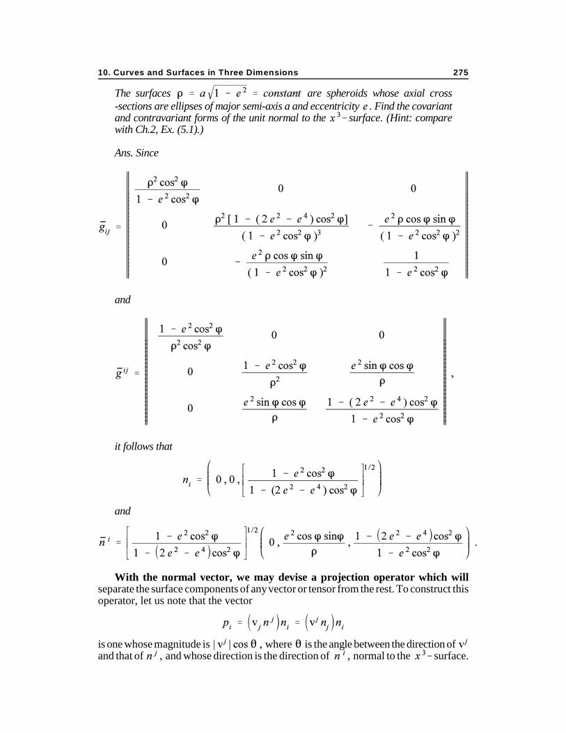
10. Curves and Surfaces in Three Dimensions 275
The surfaces are spheroids whose axial cross-sections are ellipses of major semi-axis a and eccentricity . Find the covariantand contravariant forms of the unit normal to the surface. (Hint: comparewith Ch.2, Ex. (5.1).)
Ans. Since
and
it follows that
and
With the normal vector, we may devise a projection operator which willseparate the surface components of any vector or tensor from the rest. To construct thisoperator, let us note that the vector
is one whose magnitude is where is the angle between the direction of and that of and whose direction is the direction of normal to the surface.

Chapter 4: Tensors in Generalized Coordinates in Three Dimensions276
Therefore the tensor is an operator which, when applied to any vector gives the portion of in the direction of the normal . It has the property,characteristic of projection operators, that applying it two (or more) times gives exactlythe same result as applying it once. That is,
The operator (tensor) is therefore said to be idempotent. With the normalcomponent of a vector isolated in this way, the remainder of the vector must lie inthe surface to which is the normal. Thus
(where ) is the part of which lies in the surface, i. e., the surface
components of The surface and normal projection operators are clearly orthogonal,for
Let us write out the components of . They are
(10.2)
since Clearly, has no inverse (its determinant is zero); neitherhas . This reflects the fact that a vector is not determined completely simply by itsprojection upon the surface. This projection operator is, of necessity, alsoidempotent. It may be used to find the surface components of covariant or contravariantvectors. Thus
If the vector is a surface vector, the component and the vector’s surfacecomponents in covariant form are simply Otherwise, they are as givenabove.
Similarly, the surface components of any contravariant vector are
which is clearly a surface vector.

10. Curves and Surfaces in Three Dimensions 277
Ex. (10.2) Find the surface projection operator to the surface of Ex. (10.1).
Ans. From equation (10.2) and Ex. (10.1) we have
Since any tensor may be written as the sum of products of vectors of theappropriate type, we may obtain the surface components of any tensor by applying theappropriate surface projection operator to each index. For example, the fundamentaltensor will have surface components
(10.3)
On the other hand, equation (10.2) shows that whenever or is equal to 3, theprojection must be equal to zero. Hence
Therefore
(10.4)
The surface projection of the covariant fundamental tensor takes the somewhatsurprising form
(10.5)
Chapter 4: Tensors in Generalized Coordinates in Three Dimensions278
This could have been foreseen, however, simply by lowering the indices of equations(10.3) or (10.4) It is interesting to note also that
(10.6)
Thus and are mutual inverses, since
Ex. (10.3) Derive the fundamental tensor for the surface of a spheroid by taking. (Hint: see Ex. (10.1).) Then verify the components in Ex. (10.1) by
calculating them from equation (10.4).)
Let us give application to these results by considering the Riemann-Christoffel curvature tensor. From equation (2.7.3) we have that the Riemann-Christoffeltensor is
Since there is nothing in the derivation of this result which limited it to two dimensions,it is true in three. In particular, when none of the free indices is equal to 3, we have
(Note that whereas the Greek indices have the range (1, 2), the Latin indices range from1 to 3.) Substituting from equations (10.4) and (10.5), we see that this may be writtenas

10. Curves and Surfaces in Three Dimensions 279
Now the quantity in the first two lines is the Riemann-Christoffel tensor ascalculated in the surface , treated as a two-dimensional manifold independently ofbeing the sub-space Let us designate the surface Riemann-Christoffel tensoras Then
(10.7)
where we have set
(10.8)
As we have seen, is a surface invariant. Let us therefore examine the
quantity to determine its nature under a surface transformation. Under any
transformation we must have
Therefore, under a surface transformation,
since the second partial of with respect to any pair of coordinates and vanishes in a surface transformation. Evidently, all such Christoffel symbols of thesecond kind transform as covariant tensors of the second rank under a surfacetransformation. Therefore is a doubly covariant symmetric surface tensor.
If, now, the three-dimensional space in which the surface is embedded is ordinaryEuclidean space, then
(10.9)
This relation is called the Gauss equation of the surface.
Ex. (10.4) Determine for the surface of a spheroid. (Hint: use the equation(2.7.8) and the result of Ex. (7.2) of Chapter 2.)
Ans.
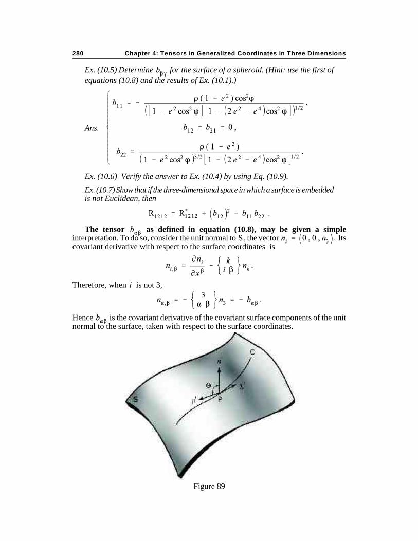
Chapter 4: Tensors in Generalized Coordinates in Three Dimensions280
Figure 89
Ex. (10.5) Determine for the surface of a spheroid. (Hint: use the first ofequations (10.8) and the results of Ex. (10.1).)
Ans.
Ex. (10.6) Verify the answer to Ex. (10.4) by using Eq. (10.9). Ex. (10.7) Show that if the three-dimensional space in which a surface is embeddedis not Euclidean, then
The tensor as defined in equation (10.8), may be given a simpleinterpretation. To do so, consider the unit normal to , the vector Itscovariant derivative with respect to the surface coordinates is
Therefore, when is not 3,
Hence is the covariant derivative of the covariant surface components of the unitnormal to the surface, taken with respect to the surface coordinates.
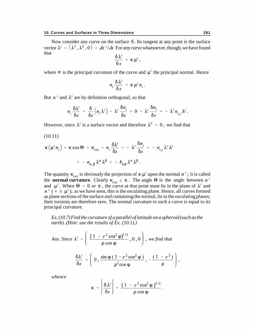
10. Curves and Surfaces in Three Dimensions 281
Now consider any curve on the surface . Its tangent at any point is the surfacevector For any curve whatsoever, though, we have foundthat
where is the principal curvature of the curve and the principal normal. Hence
But and are by definition orthogonal, so that
However, since is a surface vector and therefore we find that
(10.11)
The quantity is obviously the projection of upon the normal it is calledthe normal curvature. Clearly The angle is the angle between and When or the curve at that point must lie in the plane of and
as we have seen, this is the osculating plane. Hence, all curves formedas plane sections of the surface and containing the normal, lie in the osculating planes;their torsions are therefore zero. The normal curvature to such a curve is equal to itsprincipal curvature.
Ex. (10.7) Find the curvature of a parallel of latitude on a spheroid (such as theearth). (Hint: use the results of Ex. (10.1).)
Ans. Since we find that
whence

Chapter 4: Tensors in Generalized Coordinates in Three Dimensions282
Ex. (10.8) Find the angle between the normal to the surface of the spheroid andthe principal normal of a parallel of latitude.
Ans. From equation (10.11) and Ex. (10.4), we have
Hence from equation (10.11) and Ex. (10.7),
Let us now form the orthonormal right-handed triad and Clearly, since is orthogonal to , it therefore lies in the tangent
plane and is a surface vector. Any vector may then be conveniently resolved into a linearcombination of and In particular,
Since it follows that , and since whereas
Hence
(10.12)
where
(10.13)
We have previously found a geometric interpretation of the normal curvature The quantity the geodesic curvature, may also be given a geometricinterpretation. Thus, when the curves which are normal sections of thesurface have zero curvature and must therefore lie in a plane, the tangent plane. Then
which is evidently the curvature of the curve in the tangent plane, or thesurface curvature. More generally, curves on the surface which are not formed bynormal sections of the surface, or which do not lie in the tangent plane, will neverthelesshave curvature normal to the surface, curvature in the surface.
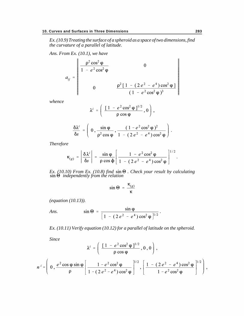
10. Curves and Surfaces in Three Dimensions 283
Ex. (10.9) Treating the surface of a spheroid as a space of two dimensions, findthe curvature of a parallel of latitude.
Ans. From Ex. (10.1), we have
whence
Therefore
Ex. (10.10) From Ex. (10.8) find . Check your result by calculating independently from the relation
(equation (10.13)).
Ans.
Ex. (10.11) Verify equation (10.12) for a parallel of latitude on the spheroid.
Since

Chapter 4: Tensors in Generalized Coordinates in Three Dimensions284
we find
Substituting these vectors into equation (10.12), we get the same results asgiven by the direct calculation in Ex. (10.7).
Ex. (10.12) Show that when the curve on the surface is the curve, then
(Hint: we have
)
Still further light may be shed upon the properties of the embedded surfaceby considering yet another aspect of the tensor . As we have seen, a symmetrictensor may have associated with it a pair of invariant eigenvalues and their associatedeigenvectors. The eigenvalues are to be found as roots of the equation
(10.14)
Suppose them to be and Then the eigenvectors are solutions of the equations
the eigenvectors will be assumed to have been normalized for convenience. If then is orthogonal to ; otherwise they may be chosen to be
orthogonal.
Let us evaluate the coefficients of the powers of in equation (10.14) . They are,respectively,

10. Curves and Surfaces in Three Dimensions 285
Now by equation (10.9) ,
On the other hand, by equation (2.7.8),
where is the Gaussian curvature. If, therefore, we set
(10.15)
the eigenvalue equation becomes
(10.16)
Calling the roots of this quadratic equation and the eigenvalues which weseek, it is evident that
(10.17)
In other words, the Gaussian curvature is the product of the two principalcurvatures of the surface, and On the other hand, the average of and
is , which is therefore called the mean curvature of the surface .
Ex. (10.13) Find the principal curvatures on the surface of a spheroid. From them,find the mean curvature and the Gaussian curvature.
Ans.
The principal curvatures have a relatively simple geometric meaning. With
them are associated the two principal directions, defined by the two mutuallyorthogonal tangent vectors and . Let and serve as an orthonormal

Chapter 4: Tensors in Generalized Coordinates in Three Dimensions286
basis for the resolution of all other surface vectors. Then any unit tangent vector which makes an angle with and with will have components inthis system given by
We then have
This is Euler’s Theorem.
If then is their common value. In general, however, we may take Then, since both and are positive,
In other words,
(10.19)
Therefore, and represent the maximum and minimum normal curvatures of allcurves at a given point. The eigenvectors and are the tangents to thesemutually orthogonal directions along which the surface curves have maximum andminimum normal curvature.
We may further note that when then
In other words, the normal curvature associated with tangent directions midway betweenthe principal directions is equal to the mean curvature. We may also note that the meancurvature vanishes only where in general, therefore, zero meancurvature does not characterize a flat space. However, if either or is zero, theGaussian curvature vanishes. Thus a plane is flat in the sense of having zero Gaussiancurvature and also in having zero mean curvature. By contrast, a cylinder or cone is flatbecause for it though its mean curvature is not zero.
The nature of the “geometry” depends upon the Gaussian curvature rather than themean curvature. As we have seen, zero Gaussian curvature characterizes the plane, inwhich Euclidean geometry holds. However, if the Gaussian curvature is positive, then
and are of the same sign; therefore the centers of curvature of all normalsections lie on the same side of the surface. The geometry of such a surface is called“elliptic” to distinguish it from plane geometry. If, however, and are of

10. Curves and Surfaces in Three Dimensions 287
opposite sign, the centers of curvature of the normal sections containing the principaldirections are on opposite sides of the surface. The geometry of such a surface is called“hyperbolic”.
Ex. (10.14) Show that for the surface of a spheroid, the vectors defining theprincipal directions are
and
Ex. (10.15) Find the Gaussian and mean curvatures of (a) a sphere, (b) a cylinder,and (c) a cone.
Ans. where a is the radius.
where a is the radius.
in a spherical coordinate system where
defines the cone, being the latitude.
Ex. (10.16) (a) Show that the unit tangent to the curve in thecoordinate system is
(b) Determine that this vector makes an angle with the unit normal, where
(c) Show that the astronomical latitude relates to the geocentriclatitude according to the formula
(d) Show from Exs. (10.8) and (10.10) that

Chapter 4: Tensors in Generalized Coordinates in Three Dimensions288
hence that where is the angle between the normal to thespheroid and the principal normal of a parallel of latitude.
Ex. (10.17) Let us define a geodesic spherical coordinate system by consideringall geodesics through a point (the origin). Along each geodesic, let the arclength be taken as the “radial” coordinate Then defines aparticular coordinate surface . At any point of construct a geodesic polarcoordinate system with coordinates and . All curves containing anypoint of an curve span an surface, etc.
11. The Riemann-Christoffel Tensor in Three Dimensions
We have defined the Riemann-Christoffel tensor in a space of twodimensions and have related it to certain of the geometric properties of a surface.
We may also define the Riemann-Christoffel tensor in three dimensions by the sameidentical equations, for there is nothing in the previous definition which implies anylimitation to two dimensions. The previous symmetries and anti-symmetries in theindices remain valid. There are now six distinct components (aside from sign) ratherthan only one, however, and in general the tensor is not isotropic. We wish to explorefurther the properties of the Riemann-Christoffel tensor.
We have noted that there are six distinct non-zero components of theRiemann-Christoffel tensor in three dimensions: they are (1) three whose indices are ofthe form (ijij), and (2) three whose indices are of the form (ikjk). Let us now show thatthese six components may be expressed in terms of the six distinct components of asymmetric second rank tensor. We put
(11.1)
Clearly called the Lamé tensor, is a second rank contravariant tensor symmetricin i and j . From it we may recover the Riemann-Christoffel tensor, for
(11.2)
Now let us form directly from a symmetric covariant tensor, namely
(11.3)
11. The Riemann-Christoffel Tensor in Three Dimensions 289
This is known as the Ricci tensor. From equation (11.1) we see that this is
where
Therefore the curvature invariant is
Hence
(11.4)
However, we can easily show that
Therefore
(11.5)
The second term on the right hand side is evidently isotropic. The Riemann-Christoffeltensor as a whole, however, is isotropic only if is zero or isotropic, henceproportional to
We may therefore ask: under what condition is the Riemann-Christoffel tensorisotropic? In general the Ricci tensor will not be zero. We must therefore require that
(11.6)
where is at most an invariant function of position. Its value may be found from therelation

Chapter 4: Tensors in Generalized Coordinates in Three Dimensions290
Consequently, Therefore the Riemann-Christoffel tensor in three dimensionswill be isotropic if and when
(11.7)
Ex. (11.1) Show that
(Hint: expand in straightforward fashion and compare the result with equation(2.7.3) of Ch.2).
Ex. (11.2) Show that
Ex. (11.3)
(Hint: take and use equation (2.7.1).)
Ex. (11.4) Show that
Ex. (11.5) Given that
(a) determine by direct calculation that
(Suggestion: calculate then etc.).

11. The Riemann-Christoffel Tensor in Three Dimensions 291
(b) Show that
(c) Show that hence that
The condition of isotropy is an even more stringent one than is apparent in
the preceding result, however, for in three (or more) dimensions it requires also that
be a constant. This is Schur’s Theorem. To prove Schur’s theorem, we appeal to the
two identities
(11.8)
and
(11.9)
The latter is known as Bianchi’s identities.
The former identity may be proven quite directly by starting from the expression for
the Riemann-Christoffel tensor in the form (see Ex. (11.1))
Then
Now
since Further,

Chapter 4: Tensors in Generalized Coordinates in Three Dimensions292
Therefore
The first term on the right hand side vanishes because of the symmetry in the parenthesisin r and s as against the antisymmetry of in r and s; the second term vanishesbecause of the symmetry of the parenthesis in q and t as against the antisymmetry of
in q and t. This proves the first identity.
To prove the Bianchi identity, we start from the fact that
Then for any covariant vector using the first expansion,
On the other hand, the second expansion gives
Equating the two expansions and using the relation
we have
After cancelling like terms on both sides, we are left with
The first term on the left is expressible in terms of the Riemann-Christoffel tensor, since is a covariant tensor of the second rank and therefore expressible as the sum of productsof two covariant vectors. Let a typical term be
11. The Riemann-Christoffel Tensor in Three Dimensions 293
Then
Since the quantity in parenthesis in the last term is symmetric in m and n, this sum overm and n must vanish. Therefore, since a sum of terms of the form
is also of this form, we see that
Therefore, making this substitution in our remaining terms, we have
We now multiply both sides of this equation by The second term on the leftvanishes, by our previous identity, equation (11.8). From the first and third terms we get
The remaining two terms on the left give
The entire left hand side therefore vanishes and we have for an arbitrary vector that
Hence
thus proving the Bianchi identities.

Chapter 4: Tensors in Generalized Coordinates in Three Dimensions294
Let us now substitute – for and write equation (11.7) as
as the form of the isotropic Riemann-Christoffel tensor. The Bianchi identity for thistensor is then
Multiplying through by we find that
Therefore
and is a constant, as Schur’s theorem states.
Ex. (11.6) Given the metric tensor
with = constant, determine whether or not the Riemann-Christoffel tensor isisotropic. (Hint: establish from the preceding and following problems that theRiemannian curvature is constant, then appeal to Schur’s Theorem.)
Ans. Since the Riemann-Christoffel tensor is isotropic.
Ex. (11.7) Show that the space in which the line element in polar coordinates is
has a constant negative curvature

11. The Riemann-Christoffel Tensor in Three Dimensions 295
Ex. (11.8) Show that the metric tensor of Ex. (11.6) can be gotten from thatof Ex. (11.5) by the transformation
Here we understand to be the coordinates of some point relative toan origin . Let be connected to by a geodesic. Then is a unit tangentto the geodesic at , hence
The quantity r is the arc length along the geodesic from to . Thus the areboth the coordinates of the point and the components of the position vector of
. The quantity k is
Ans. First we have
Then
whence
and
so that

Chapter 4: Tensors in Generalized Coordinates in Three Dimensions296
Therefore
Ex. (11.9) Derive the line element of Ex. (11.7) from that of Ex. (11.5) by atransformation analogous to that of Ex. (11.8).
Ex. (11.10) In three dimensions, both the Ricci tensor and the Riemann-Christoffeltensor have six distinct components. Therefore solve equation (11.3) for theRiemann-Christoffel tensor.
Ans.
where
Appendix 4.1 : The Advance of Perihelion
From Exs. (3.4) and (3.5) we have as the equation of motion

Appendix 4.1: The Advance of Perihelion 297
where we have made use of the fact that Here is the mass of theprimary (sun) and m the mass of the much smaller secondary (planet). Guided by thewell-known solution to the two-body problem, we recognize that there is no loss ofgenerality in taking the coordinate system to be such that the orbital plane is the plane Then the third equation is automatically satisfied and the second becomes
where a is the major semi-axis of the orbital ellipse, e the eccentricity, and the periodof revolution. With this integral, we eliminate derivatives with respect to t in favor ofderivatives with respect to according to the equation
Then the first equation takes the form
Here primes denote derivatives with respect to . Since we seek asolution of the form
Then
The first of these has the well-known Keplerian solution
where for elliptical motion and corresponds to the position ofperihelion. Substituting this expression for into the second equation gives
Solving this equation by any standard method, such as variation of parameters, andimposing the initial conditions for perihelion, we find that

Chapter 4: Tensors in Generalized Coordinates in Three Dimensions298
Hence
where
Since
we write the solution in the final form
In the ordinary Keplerian solution, the secondary returns to perihelion after onesidereal revolution, i. e. when However, in this instance we see that
In other words, the secondary falls short of its perihelion position by an angle this is another way of saying that the perihelion has advanced by radians. For theplanet Mercury, amounts to 43”/century.
Appendix 4.2 The Two-Center Problem
The gravitational potential function V, in the bipolar coordinates of Fig. 33 (orFig. 76), is clearly
Since the potential functiontherefore becomes
On the other hand, the kinetic energy is (see Ex. 2.1.8)
Appendix 4.2: The Two-Center Problem 299
Hence
Writing Lagrange’s equations in the form
we have when i = 1 that
When i = 2 we get the corresponding equation
To solve these equations, we multiply the first by the second by and add. Thisgives
After collecting terms and integrating, this becomes
(A4.2.1)
where is a constant, identifiable as the total energy.
Next, we multiply the first equation by
Chapter 4: Tensors in Generalized Coordinates in Three Dimensions300
Then
Integrating both sides, we get
(A4.2.2)
where is a second constant of integration.
We now write equation (A4.2.1) in the form
Subtracting equation (A4.2.2) from this gives
(A4.2.3)
Notes – Chapter 4 301
From equations (A4.2.2) and (A4.2.3) it is clear that
The trajectory of the mass m is given implicitly by the integrals
while the motion is determined by the integral
Notes - Chapter 4
§4.2 For a thorough treatment of the properties of space curves, see Laugwitz (8),Ch. I. Among the results of interest are:
(i) A curve is a plane curve if and only if its torsion vanishes.
(ii) In the neighborhood of a point on a curve whose parameter value is , theposition vector has the canonical expansion
through the third order in It is illuminating to interpret the contribution of eachorder of
(iii) To within a rigid body displacement, the functions and determineuniquely the curve for which and s are the curvature, torsion, and arclength, respectively. This is the content of what is known as the FundamentalTheorem of the theory of curves in Euclidean 3-space.
§4.3 (a) A detailed discussion of the derivation of the Euler-Lagrange equations undera wide variety of conditions and of their application to many problems of particle andcontinuum mechanics is given a model exposition in Lanczos (7).
(b) Many concrete, sophisticated applications of the Euler-Lagrange method are workedout fully in Wells (21).
Chapter 4: Tensors in Generalized Coordinates in Three Dimensions302
(c) Whittaker (24) describes a formulation of the potential and kinetic energies by A. G.Walker which reduces to the traditional forms in the limit as the velocity of light and yet which may be used with the classical Euler-Lagrange equations to derive thestandard results of both special and general relativity, including the advance ofperihelion and the gravitational refraction (see App. 4.1 and App. 6.1).
(d) The great utility and frequent economy of curvilinear coordinates is sometimes offsetin part by the difficulty of translating the components of vector or tensor quantities inthese coordinates into terms which may readily be apprehended physically. Even thedimensions of physical quantities may depend upon the choice of coordinate system; afamiliar case in point is velocity, whose components are all linear in Cartesiancoordinates but include angular components in spherical coordinates. For physicalapplications it is therefore frequently desirable to define the physical components ofa vector or tensor. If is a unit vector in any direction, then is the physicalcomponent of the vector in the direction of . By the use of the Product Theorem,one can readily define physical components for tensors of any order and type. For amore detailed discussion of the matter, see Synge and Schild (18), §5.1, pp. 142-149.
§4.4 (a) For other, more extensive expositions of geometrical dynamics, see Laugwitz(8), §14, pp. 167-176; McConnell (9), pp. 246-249; or Synge and Schild (18), §5.5, pp.168-184.
(b) Closely related to geometrical dynamics is the content of Helmholtz’ Theoremwhich states that if there is free mobility of rigid bodies of any finite extension,then the space is Riemannian of constant curvature. For a proof of this theorem, seeLaugwitz (8), pp. 183-184.
§§4.3-4.4 Detailed consideration of many common problems in the mechanics ofparticles and rigid bodies will be found in Spiegel (16).
§4.5 Generalizations of the theorems of Green and Stokes as well as a discussion ofrelative tensors (as opposed to absolute tensors, to which we have confined ourdiscussion) may be found in Synge and Schild (18), Ch. VII, pp. 240-281. Detaileddiscussion of divergence, curl, and Laplacian will be found in Davis (4), §§3.3-3.6, pp.97-116.
The jump discontinuity referred to in Ex. (5.12) may be defined by saying that avector is said to have a jump discontinuity on a surface if there are two continuous
points near onvectors and defined over and such that the values of at the values of one side approach the values of and on the other side approach
§4.6 Strain, rigid body displacements, and infinitesimal deformations are discussed inMcConnell (8), Ch. X, pp. 120-128 and in Synge and Schild (18), §§5.3-5.4, pp.156-168.
§4.8 P. W. Bridgman, in his The Logic of Modern Physics (Macmillan, New York,1949, pp. 56-57), offers some very a propos comments on the subject of fields whichmay be applied more generally to all fields. They are worth quoting at length:

Notes – Chapter 4 303
“[A]n examination of the operations by which we determine the electric field at any point will
show that it is a construct, in that it is not a direct datum of experience. To determine the electric
field at any point, we place an exploring charge at the point, measure the force on it, and then
calculate the ratio of the force to the charge. We then allow the exploring charge to become
smaller and smaller, repeating our measurement of force on each smaller charge, and define the
limit of the ratio of the force to the charge as the electric field intensity at the point in question,
and the limiting direction of the force on a small charge as the direction of the field. We may
extend this process to every point of space, and so obtain the concept of a field of force, by which
every point of the space surrounding electric charges is tagged with the appropriate number and
direction, the exploring charge having completely disappeared.
“The field is, then, clearly a construct. Next, from the formal point of view of mathematics, it is
a good construct, because there is a one to one correspondence between the electric field and the
electric charges in terms of which it is defined, the field being uniquely determined by the charges,
and conversely there being only one possible set of charges corresponding to a given field. Now
nearly every physicist takes the next step, and ascribes physical reality to the electric field, in that
he thinks that at every point of the field there is some real physical phenomenon taking place
which is connected in a way not yet precisely determined with the number and direction which
tag the point. At first this view most naturally involved as a corollary the existence of a medium,
but lately it has become the fashion to say that the medium does not exist, and that only the field
is real. ... I believe that a critical examination will show that the ascription of physical reality to
the electric field is entirely without justification. I cannot find a single physical phenomenon or
a single physical operation by which evidence of the existence of the field may be obtained
independent of the operations which entered the definition. ...
“It seems to me that any pragmatic justification in postulating reality for the electric field has now
been exhausted, and that we have reached a stage where we should attempt to get closer to the
actual facts by ridding the field concept of the implication of reality.”
§4.9 For the equations of electromagnetism in matter, see McConnell (9), Ch. XIX, pp.255-270.
§4.10 (a) For an alternative treatment of surfaces and curves on surfaces, see (i)Laugwitz (8), Ch. II, pp. 19-78; (ii) Kreyszig (5), Chs. III-VIII; and (iii) McConnell (9),Chs. XIV - XVI. These references also include discussions of many interesting mattersnot covered here, such as ruled and developable surfaces, minimal surfaces, andenvelopes ; reference (ii) , in particular, includes many problems, with answers toodd-numbered exercises.
(b) Orientable surfaces are discussed in Kreyszig (5), p. 108, Synge and Schild (18), p.261; and Davis (4), §4.5, pp. 151-160. All infinitesimal surface elements are orientable.Extended surfaces may not be orientable; the Moebius strip is a familiar example.
(c) See Note 1.15 (b) concerning projection operators.
(d) If a surface contains a straight line, that straight line is a geodesic curve on thesurface. (Laugwitz (8), p. 45).

Chapter 4: Tensors in Generalized Coordinates in Three Dimensions304
(e) A second very important relation for a surface, in addition to Gauss’ equation, is theequation of Codazzi. We may easily derive it by noting that
If, therefore, 3-dimensional space is flat, so that
But if then either or Let . Then
These are the equations of Codazzi.
(f) The fundamental theorem of the theory of surfaces states that the surface tensor assumed to be positive definite (i. e., if and togetherdetermine a surface uniquely to within a rigid body displacement if they satisfy both theequations of Gauss and of Codazzi. For a more extended discussion, see Laugwitz (7),§11.07, or Sokolnikoff (14), pp. 184-186. In the former reference, it is noted (p. 131)that although the and determine a surface, these quantities are neitherindependent nor scalar. The problem of finding a complete set of invariants which fullycharacterize a surface is indeed a very difficult one, unlike the analogous problem forcurves (see Note 4.2).
§4.11 (a) It is shown in Adler, Bazin, and Schiffer (1), pp. 81-83, that for any vector it is identically true that
(b) It is shown in Sokolnikoff (14), pp. 92-96, that the necessary and sufficient conditionthat a geometry be Euclidean is that the Riemann-Christoffel tensor vanish. Schrödinger(13), pp. 43-52, relates the Riemann-Christoffel tensor to integrability about closedpaths. This is the celebrated Pfaffian problem.
(c) Spaces of constant curvature are discussed in Synge and Schild (18), Ch. IV, andLaugwitz (8), §12.
(d) Laugwitz (8), p.127, interprets the curvature invariant in dimensions as
times the arithmetic mean of all the Riemannian curvatures belonging to the planardirections which are obtainable from mutually orthogonal vectors.