Chapter 30:The Labor Market

Copyright © 2013 by The McGraw-Hill Companies, Inc. All rights reserved.McGraw-Hill/Irwin

13e

30-2

The Labor Market

• There isn’t just one labor market because everyone is not qualified to do every job.

• Some jobs pay more, some jobs pay less.• As with any market, the various labor

markets are governed by the supply of labor and the demand for labor. And the market will determine the price of labor – that is, the wage.

30-3

Learning Objectives

• 30-01. Know what factors shape labor supply and demand.

• 30-02. Know how market wage rates are established.

• 30-03. Know how wage floors alter labor market outcomes.

30-4

Labor Supply

• Labor supply: the willingness and ability to work specific amounts of time at alternative wage rates in a given time period.– As with any supply of anything, people, in

general, will be willing to work more hours if the pay is higher and fewer hours if the pay is lower, ceteris paribus.

– In addition to being paid for work, there is also an intrinsic satisfaction one gets from working.

30-5

Labor Supply

• There is value in not working, too. It is called enjoying leisure time.– Economists divide your time into work hours

and leisure hours. The two together add up to 24 hours a day.

– The opportunity cost of working more hours is the value you place on the leisure hours you give up to work those extra hours.

30-6

Labor Supply• If you have 24 hours of leisure, taking a job

requires you to give up some of those hours.– The opportunity cost of doing so is very low.

• As you increase work hours, you must give up leisure hours that are more valuable to you.– As work hours increase, the opportunity cost rises

rapidly as leisure hours become more scarce.– You will require a higher wage to compensate for

this increasing opportunity cost. This is the basis for overtime pay.

30-7

Labor Supply

• Therefore, we will supply more labor hours only if offered a higher wage.– The labor supply curve slopes upward.

• From a marginal utility (MU) point of view, the first few dollars you earn have a very high MU, but as you work more hours and earn more money, the MU of income may decline.– This reinforces the need for a higher wage to get us

to work more hours.

30-8

Labor Supply• At some wage, even more wages may not

induce us to work more hours.• In fact, increased wages may induce us to work

fewer hours, not more:– Say, each week you earn $10 an hour working 60

hours, or a total of $600. This amount is enough to fund your lifestyle.

– Now you are offered a raise to $15 an hour. It is possible you would cut back to 40 hours and earn $600. You increase your leisure time by 20 hours.

30-9

Labor Supply• There are two effects in operation here:– Substitution effect of higher wages: an increased

wage rate encourages people to work more hours (substitute labor for leisure).

– Income effect of higher wages: an increased wage rate allows a person to reduce hours worked without losing income.

• At low wages, the substitution effect dominates; at high incomes, the income effect dominates.

30-10

Labor Supply• The resulting labor

supply curve bends backward.

• The wage rate where the income effect begins to dominate is where the curve begins to bend backward.

30-11

Market Supply• The market supply of labor is the collective

individual labor supply.• The market supply curve will shift if any

determinant changes:– Tastes (for leisure, income, and work).– Income and wealth.– Expectations (of a change in income or

consumption requirement).– Prices (of consumer goods).– Taxes.

30-12

Elasticity of Labor Supply

• Consider day laborers or any low-skill job.– How many people are currently qualified to do

the work?– Of those, how many are currently available to be

hired?– How long is the “pipeline” – that is, the time

required to become qualified to do the job?

30-13

Elasticity of Labor Supply

• For low-skill jobs, the supply of labor is large and the time to qualify is short.

• A very small % increase in the wage rate would generate a large % increase in applicants.– For low-skill jobs, labor supply is highly elastic.

30-14

Elasticity of Labor Supply

• Consider surgery nurses or any high-skill job.– How many people are currently qualified to do

the job?– Of those, how many are currently available to be

hired?– How long is the “pipeline” – that is, the time

required to become qualified to do the job?

30-15

Elasticity of Labor Supply

• For high-skill jobs, the supply of labor is small and the time to qualify is long.

• A large % increase in the wage rate would generate a small % increase in applicants.– For high-skill jobs, labor supply is highly

inelastic.

30-16

Labor Demand• Labor demand: the quantities of labor

employers are willing and able to hire at alternative wage rates in a given time period.– Labor demand is not independent. Firms don’t hire

just to have people around.– Labor demand is a derived demand – that is, it is

derived from the demand for the goods and services being made.

• Firms will be willing to hire more workers at low wage rates and fewer workers as wage rates rise.

30-17

Labor Demand

• Labor is a factor input to the process used to generate a salable product.

• The value to the firm of an added worker is related to the added sales revenue –marginal revenue (MR) – received when the added output is sold.

• The added output a new hire can produce is called marginal physical product (MPP).

30-18

Labor Demand

• Put these two ratios together to get the dollar value of a worker’s contribution to the firm’s output: marginal revenue product (MRP).

Change in total revenue Marginal revenue (MR) = Change in output

Change in outputMarginal physical product (MPP) = Change in quantity of labor

30-19

Labor Demand• Assume the firm can sell all its output at the

market price, so MR = p.• The value of a worker, MRP, is equal to the

product of price (p) and marginal physical product (MPP).

Change in total revenue Marginal revenue product = Change in quantity of labor

MRP = MPP X p

30-20

Labor Demand• Marginal revenue product (MRP) sets the

upper limit to the wage an employer will pay.• MRP is subject to the law of diminishing

returns.– As more workers are hired, MPP begins to diminish

because capital is fixed in the short run.

• As MPP diminishes, so does MRP. – Recall that MRP = MPP X p

• MRP is the firm’s demand curve and slopes downward.

30-21

The Hiring Decision• Compare benefit to cost.• The benefit is MRP; the

cost is the wage rate.• If MRP > wage (point B),

add workers and profit rises.

• If MRP < wage (point D), lay off workers and profit rises.

• The ideal number of workers exists where MRP = wage (point C), where profit is maximized.

30-22

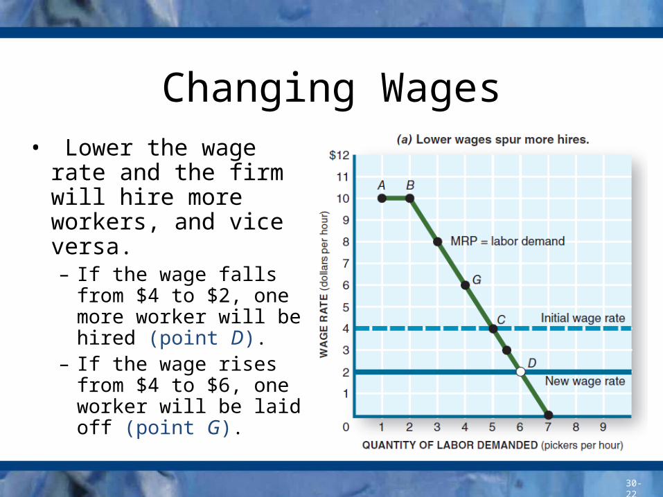
Changing Wages• Lower the wage rate

and the firm will hire more workers, and vice versa.– If the wage falls from

$4 to $2, one more worker will be hired (point D).

– If the wage rises from $4 to $6, one worker will be laid off (point G).

30-23

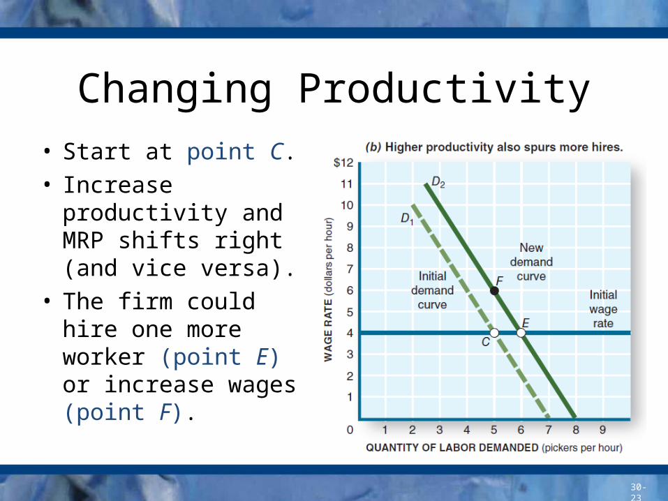
Changing Productivity• Start at point C. • Increase

productivity and MRP shifts right (and vice versa).

• The firm could hire one more worker (point E) or increase wages (point F).

30-24

Labor Market Equilibrium

• The intersection of labor market demand and labor market supply sets the equilibrium wage.

• At this rate, the quantity of labor supplied equals the quantity of labor demanded.– Above this rate, there is a surplus of labor.– Below this rate, there is a shortage of labor.

30-25

Minimum Wage• A government-

imposed minimum wage is set at WM, above the market wage of We.

• A surplus is created.• Some workers (0 to

qd) benefit with higher pay; some lose their jobs (qd to qe); some start looking but can’t find jobs (qe to qs).

30-26

Minimum Wage• A minimum wage– Reduces the quantity of labor demanded.– Increases the quantity of labor supplied.– Creates a market surplus.

• A minimum wage increase makes all three results worse.

• The minimum wage applies mainly to the low-skill end of the labor market, so supply is highly elastic. Firms cut jobs at a greater rate than the minimum wage increase.

30-27

Choosing among Inputs

• When deciding whether to hire more labor or to add more capital, a firm will compare the cost efficiency of each.– Cost efficiency: the amount of output associated

with an additional dollar spent on an input; the MPP of an input divided by its price (or cost).

– The most cost-efficient input is the one that produces the most added output per dollar.

30-28

Choosing among Inputs

• Compare MPP/P for labor to MPP/P for capital.– If labor is more cost-efficient, add workers and

the process becomes more labor-intensive.• In countries where labor is cheap and capital is

expensive, work is labor-intensive.

– If capital is more efficient, add capital and the process becomes more capital-intensive.• In countries where labor is expensive and capital is

cheap, work is capital-intensive.