Chapter 30 MSMYP1 Further Complex Variable Theoryigor.gold.ac.uk/~mas01rwb/notes/YP1.pdf · Chapter...
18
Chapter 30 MSMYP1 Further Complex Variable Theory (30.1) Multifunctions A multifunction is a function that may take many values at the same point. Clearly such functions are problematic for an analytic study, though for the most part there is a convenient way to prevent their bad behaviour. Unfortunately some functions of R → R become multifunctions when extended to C, so first of all these are dealt with. (30.1.1) Arguments Representing a complex number in the form z = re iθ , the argument of z is the number θ which gives the angle (in radians) that a line segment connecting the origin to z makes with the positive real axis. For a given complex number z = re iθ there are many arguments, namely θ ± 2kπ for k ∈ Z. Let ARG(z) = θ | z = re iθ Any one of the elements of ARG(z) may be chosen for use, so let arg (z) ∈ ARG(z), which may also be treat as a function arg (z): C \{0}→ R arg (z) is called a choice for ARG(z), and no choice is a continuous function. This is simply demonstrated by noting that any continuous function is continuous when restricted to any contour. Choosing the unit circle as a contour, γ : [0, 1) → C defined by γ : t → e it Plotting the function arg (z) on a third axis (see Figure 30.1.1) there is clearly a discontinuity where the function returns to the positive real axis. The problems with the argument function occur when the positive real axis is crossed, and so can be solved by removing the positive real axis from C. In fact any half-line can be removed, so define L α = z ∈ C | z = re iα ∀r 0 In the cut plane C \ L α the choice arg (z) ∈ (α, α + 2π) is continuous. 1
Transcript of Chapter 30 MSMYP1 Further Complex Variable Theoryigor.gold.ac.uk/~mas01rwb/notes/YP1.pdf · Chapter...
Chapter 30
MSMYP1 Further Complex Variable
Theory
(30.1) Multifunctions
A multifunction is a function that may take many values at the same point. Clearly such functions areproblematic for an analytic study, though for the most part there is a convenient way to prevent their badbehaviour. Unfortunately some functions of R→ R become multifunctions when extended to C, so first ofall these are dealt with.
(30.1.1) Arguments
Representing a complex number in the form z = reiθ , the argument of z is the number θ which gives theangle (in radians) that a line segment connecting the origin to z makes with the positive real axis. For agiven complex number z = reiθ there are many arguments, namely θ ± 2kπ for k ∈ Z. Let
ARG(z) ={
θ | z = reiθ}
Any one of the elements of ARG(z) may be chosen for use, so let arg (z) ∈ ARG(z), which may also be treatas a function
arg (z) : C \ {0} → R
arg (z) is called a choice for ARG(z), and no choice is a continuous function. This is simply demonstrated bynoting that any continuous function is continuous when restricted to any contour. Choosing the unit circleas a contour,
γ : [0, 1)→ C defined by γ : t 7→ eit
Plotting the function arg (z) on a third axis (see Figure 30.1.1) there is clearly a discontinuity where thefunction returns to the positive real axis.
The problems with the argument function occur when the positive real axis is crossed, and so can be solvedby removing the positive real axis from C. In fact any half-line can be removed, so define
Lα ={
z ∈ C | z = reiα ∀r > 0}
In the cut plane C \ Lα the choicearg (z) ∈ (α, α + 2π)
is continuous.
1

2 CHAPTER 30. MSMYP1 FURTHER COMPLEX VARIABLE THEORY
Figure 1: The argument function is not continuous.
(30.1.2) Logarithms
As complex numbers have expressions in terms of exponentials it is important that any definition of alogarithm is consistent with this.
z = |z|ei arg (z)
= eln |z|ei arg (z)
= exp (ln |z|+ i arg (z))
Hence make the definitionlnz = ln|z|+ i arg (z)
The appearance of the argument function makes this a multifunction. Similarly to the argument, let
LOG(z) = {ln |z|+ iθ | θ ∈ ARG(z)}
However, in the cut plane C \ Lα, ln z is a sum of continuous functions and thus is continuous. In fact ln zis analytic. Each possible cut of the complex plane gives rise to an analytic logarithm function, all of whichare different. It is therefore common to speak of an “analytic branch of the logarithm” corresponding to aparticular cut. Of course, it is most convenient to use the cut C \ L0.

30.2. POLES AND ZEROS 3
(30.1.3) Powers
For w, z ∈ C
zw = exp (w ln z)
and thus exponentiation is a multifunction. Obviously cutting the plant will eliminate this problem.
(30.2) Poles And Zeros
The zeros and poles of a function f : C→ C are of interest.
Suppose that f is analytic and has a zero at z0, then for some r > 0 f has a Taylor expansion about z0 onBr(b0) as follows
f (z) = cm(z− z0)m + cm+1(z− z0)m+1 + . . .
= (z− z0)m∞
∑k=0
cm+k(z− z0)k
= (z− z0)mg(z)
where g is analytic on and has no zeros in Br(z0). When f can be expressed in this way it is said to have azero of order (or multiplicity) m at z0.
Similarly, if f has a pole of order (or multiplicity) n at p0 then it has a Laurent expansion on Br(p0 for somer > 0, say
f (z) =c−n
(z− p0)n +c−n+1
(z− p0)n−1 + · · ·+ c−1z− p0
+ c0 + . . .
=1
(z− p0)n
∞
∑k=0
c−n+k(z− p0)k =g(z)
(z− p0)n
where g is analytic on and has no zeros in Br(p0).
Theorem 1 (Principle Of The Argument) Let U be an open simply connected domain and γ be a positively orientedcontour in U. If f : U → C is analytic on U except at finitely many points (poles) and has finitely many zeros in Uthen
12πi
∫γ
f ′(z)f (z)
dz = N − P
where f has N zeros and P poles in U.
Proof. Let p1, p2, . . . , pk be the poles of f inside γ, with the ith having multiplicity ni. Let z1, z2, . . . , zl be thezeros of f inside γ, with the jth having multiplicity mj. Choose r > 0 such that
f (z) = (z− zj)mjgj(z) ∀z ∈ Br(zj)
and f (z) = (z− pi)−ni gl+i(z) ∀z ∈ Br(pi)
where each g is non-zero and analytic on its respective ball. As there are only finitely many poles and zeros,r may be chosen small enough to make all the balls disjoint.
4 CHAPTER 30. MSMYP1 FURTHER COMPLEX VARIABLE THEORY
Take any j (1 6 j 6 k) then in Br(zj)
f (z) = (z− zj)mj gj(zj)
so f ′(z) = mj(z− zj)mj−1 + (z− zj)
mj g′j(zj)
givingf ′(z)f (z)
=mj
z− zj+
g′j(z)
gj(z)
=mj
z− zj+ h(z)
where h is analytic on Br(zj). This function has a single pole at zj with residue mj. Similarly, take any i(1 6 i 6 l) then in Br(pi)
f (z) = (z− pi)−ni gl+i(zi)
so f ′(z) = −ni(z− pi)−ni−1 + (z− pi)
−ni g′l+i(zi)
givingf ′(z)f (z)
=−ni
z− pi+
g′l+i(z)gl+i(z)
=ni
z− pi+ h(z)
where h is analytic on Br(pi). This function has a single pole at pi with residue −ni. Now, poles of f ′(z)f (z) can
occur only at poles of f ′ (which must be poles of f ) and zeros of f . Thus by Cauchy’s Residue Formula
12πi
∫γ
f ′(z)f (z)
dz =k
∑i=1−ni +
l
∑j=1
mj = N − P�
Corollary 2 N − P =1
2πi4
gammaarg f (z)
Proof.
N − P =1
2πi
∫γ
f ′(z)f (z)
dz
=1
2πi
∫ b
a
f ′(γ(t))f (γ(t))
γ′(t) dt
=1
2πi[ln ( f (γ(t)))]ba
=1
2πi(ln | f (γ(b))|+ i arg ( f (γ(b)))− f (γ(a))|+ i arg ( f (γ(a))))
=1
2πi( arg ( f (γ(b)))− arg ( f (γ(a))))
=1
2πi4γ
arg f (z)
where4γ arg f (z) denotes the change around γ of the argument of f (z). �
This corollary suggests why the theorem is called the “Principle Of The Argument”.
Applying a root-counting argument in fact allows a proof of the Fundamental Theorem of Algebra, a proofnormally in the realm of algebra. Firstly, a lemma.
Lemma 3 If h(z) = c1z + c2
z2 + · · ·+ cnzn for constants ci, then ∃R > 0 such that |h(z)| < 1 for z > R.
30.2. POLES AND ZEROS 5
Proof. Using first the triangle inequality,
|h(z)| 6 |c1||z| +
|c2||z|2 + · · ·+ |cn|
|z|n
6 max16i6n
{|ci}(
1|z| +
1|z|2 + · · ·+ 1
|z|n
)6 max
16i6n{|ci}
n|z|
with the last line following when |z| > 1. Hence choosing R > max{1, n max{|ci|}} the result is obtained.�
Theorem 4 (Fundamental Theorem Of Algebra) If p(z) ∈ C[z] is of order n > 1 then p has precisely n zeros in C.(More simply: C is algebraically closed.)
Proof. Let p(z) = a0 + a1z + · · ·+ anzn then p is entire. Write
p(z) = anzn(1 + f (z))
with f (z) =an−1
an
1z
+an−2
an
1z2 + · · ·+ a0
an
1zn
By Lemma 3 ∃R > 0 such that |z| > R ⇒ | f (z)| < 1. But then 1 + f (z) 6= 0 and certainly z 6= 0 so that phas no roots outside the contour |z| = R, and no roots on the contour either.
Now, 1 > | f (z)| = |(1 + f (z))− 1| so 1 + f (z) lies in the unit circle centred at 1. Therefore −π2 < arg (1 +
f (z)) < π2 and so
0 6
∣∣∣∣∣ 4|z|=R(1 + f (z))
∣∣∣∣∣ 6 π
Applying the Principle Of The Argument, this must be an integer multiple of 2π, and thus is zero. Hence
4|z|=R
p(z) = 4|z|=R
( arg anzn) + 4|z|=R
( arg (1 + f (z)))
= 4|z|=R
arg anzn
= 4|z|=R
arg an|z|neinθ
= 2nπ
By the Principle Of The Argument p has n roots and poles inside |z| = R, but as p has no poles it has nzeros, all in C. �
Zeros and poles can also be counted by looking at the behaviour of functions on a contour. Where N f
denotes the number of zeros of f and Pf denotes the number of poles of f :
Theorem 5 (Generalised Rouche) Let U be a simply connected open domain and let γ be a positively oriented simplyconnected closed contour in U. Let f and g be analytic on U, except for finitely many poles inside γ. If |g(z)| < | f (z)|for all z on γ then
N f − Pf = N f +g − Pf +g
Proof. For functions f and g as described, consider
F =f (z)
f (z) + g(z)
6 CHAPTER 30. MSMYP1 FURTHER COMPLEX VARIABLE THEORY
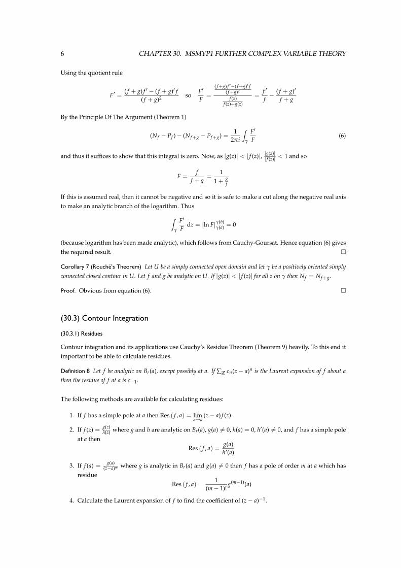
Using the quotient rule
F′ =( f + g) f ′ − ( f + g)′ f
( f + g)2 soF′
F=
( f +g) f ′−( f +g)′ f( f +g)2
f (z)f (z)+g(z)
=f ′
f− ( f + g)′
f + g
By the Principle Of The Argument (Theorem 1)
(N f − Pf )− (N f +g − Pf +g) =1
2πi
∫γ
F′
F(6)
and thus it suffices to show that this integral is zero. Now, as |g(z)| < | f (z)|, |g(z)|| f (z)| < 1 and so
F =f
f + g=
11 + g
f
If this is assumed real, then it cannot be negative and so it is safe to make a cut along the negative real axisto make an analytic branch of the logarithm. Thus
∫γ
F′
Fdz = [ln F]γ(b)
γ(a) = 0
(because logarithm has been made analytic), which follows from Cauchy-Goursat. Hence equation (6) givesthe required result. �
Corollary 7 (Rouche’s Theorem) Let U be a simply connected open domain and let γ be a positively oriented simplyconnected closed contour in U. Let f and g be analytic on U. If |g(z)| < | f (z)| for all z on γ then N f = N f +g.
Proof. Obvious from equation (6). �
(30.3) Contour Integration
(30.3.1) Residues
Contour integration and its applications use Cauchy’s Residue Theorem (Theorem 9) heavily. To this end itimportant to be able to calculate residues.
Definition 8 Let f be analytic on Br(a), except possibly at a. If ∑Z cn(z− a)n is the Laurent expansion of f about athen the residue of f at a is c−1.
The following methods are available for calculating residues:
1. If f has a simple pole at a then Res ( f , a) = limz→a
(z− a) f (z).
2. If f (z) = g(z)h(z) where g and h are analytic on Br(a), g(a) 6= 0, h(a) = 0, h′(a) 6= 0, and f has a simple pole
at a thenRes ( f , a) =
g(a)h′(a)
3. If f (a) = g(a)(z−a)m where g is analytic in Br(a) and g(a) 6= 0 then f has a pole of order m at a which has
residueRes ( f , a) =
1(m− 1)!
g(m−1)(a)
4. Calculate the Laurent expansion of f to find the coefficient of (z− a)−1.

30.3. CONTOUR INTEGRATION 7
5. Calculate the integral c−1 =1
2πi
∫γ
f (z) dz.
The most frequently applicable of these is, unfortunately, the rather tedious method 4. To this end it is worthnoting the following expansions
11− z
=∞
∑n=0
zn ez =∞
∑n=0
zn
n!sin z =
∞
∑n=0
(− 1)nz2n+1
(2n + 1)!cos z =
∞
∑z=0
(− 1)nz2n
(2n)!
A useful trick with these is as follows:
cosec (πz) =1
sin (πz)
=1
πz− (πz)3
3! + (πz)5
5! − . . .
=1
πz1
1− (πz)2
3! + (πz)4
5! − . . .
=1
πz1
1−(
(πz)2
3! −(πz)4
5! + . . .)
=1
πz
∞
∑n=0
((πz)2
3!− (πz)4
5!+ . . .
)n
=1
πz+
1πz
((πz)2
3!− (πz)4
5!+ . . .
)+
1πz
((πz)2
3!− (πz)4
5!+ . . .
)2
+ . . .
from which the coefficient of z−1 can be calculated.
Contour integrals may easily be evaluated by use of the following theorem.
Theorem 9 (Cauchy’s Residue Theorem) Suppose that γ is a simple closed contour in a domain D, and let f be acomplex function which is analytic on D except at finitely many points, p1, p2, . . . , pk, all of which line in Int γ. Then
∫γ
f (z) dz = 2πik
∑i=1
Res ( f , pi)
There are a few common choices of contour, each useful for integrating certain kinds of function. These arenow examined by means of example.
(30.3.2) Semi-Circular Contours
Semi-circular contours are useful for evaluating real improper integrals of functions that behave badly atcertain points in R.
Example 10 Evaluate∫ ∞
0
ln xa2 − x2 dx (a > 0) by integrating round a suitable complex contour.
Proof. Solution Use the contour shown in Figure 2, where
1. γ1 is a contour along the positive real axis from ε to R, so on γ1 z = x.
2. γ2 is a semicircular contour centred at the origin and of radius R, so on γ2 z = Rei arg θ for 0 6 θ 6 π.
3. γ3 is a contour along the negative real axis from −R to −ε. Here, arg z = π so that on γ3 z = xeiπ .
4. γ4 is a semicircular contour centred at the origin and of radius ε, so on γ4 z = εeiθ for 0 6 θ 6 π.

8 CHAPTER 30. MSMYP1 FURTHER COMPLEX VARIABLE THEORY
-
Im z6
Re z
γ2AK
γ1-γ3- γ4
Figure 2: Contour of integration for use in evaluating improper real integrals with singularities.
Refer to the whole contour as ΓR,ε and consider the function f (z) = ln xa2−x2 . As a contour cannot cross a cut,
define an analytic branch of the logarithm function by cutting from the plane the negative imaginary axis,so that arg z ∈
(−π
2 , 3π2
). The only pole lying inside the contour is at ia, and for it to lie inside the contour
it is required that ε < a < R. This pole has residue
Res ( f , ia) =1
2ia
(ln a + i
π
2
)Now go about evaluating
∫ΓR,ε
f (z) dz with the eventual aim of applying Theorem 9.
• On γ1 z = x so ∫γ1
f (z) dz =∫ R
ε
ln xa2 + x2 dx = IR,ε, say
• On γ3 z = xeiπ so
∫γ3
f (z) dz =∫ z=−ε
z=−R
ln(
xeiπ)
a2 − x2e2iπ eiπ dx
= −∫ x=ε
x=R
ln(
xeiπ)
a2 − x2 dx
=∫ R
ε
ln(
xeiπ)
a2 − x2 dx
=∫ R
ε
ln x + iπa2 − x2 dx
= IR,ε +∫ R
ε
iπa2 + x2 dx
• On γ2 z = Reiθ for 0 6 θ 6 π so
∣∣∣∣∫γ2
f (z) dz∣∣∣∣ =
∣∣∣∣∣∣∫ π
0
ln(
Reiθ)
a2 + R2e2iθ Reiθ dθ
∣∣∣∣∣∣6∫ π
0
∣∣∣∣∣∣ln(
Reiθ)
a2 + R2e2iθ Reiθ
∣∣∣∣∣∣ dθ
=∫ π
0
| ln R + iθ||Reiθ |∣∣a2 + R2e2iθ∣∣ dθ

30.3. CONTOUR INTEGRATION 9
Now, the denominator describes a circle centred at a2 and of radius R2. The minimum distance fromthe origin to this circle occurs when the circle crosses the real axis near the origin. Since R2 > a2 thisgives
6∫ π
0
| ln R + iθ||Reiθ |R2 − a2 dθ
6∫ π
0
(| ln R|+ θ)RR2 − a2 dθ by the triangle inequality and since R > 0
6∫ π
0
(| ln R|+ π)RR2 − a2 dθ
=π(| ln R|+ π)R
R2 − a2
→ 0 as R→ ∞
• On γ4 z = εeiθ for 0 6 θ 6 π so
∣∣∣∣∫γ4
f (z) dz∣∣∣∣ =
∣∣∣∣∣∣∫ 0
π
ln(
εeiθ)
a2 + ε2e2iθ εeiθ dθ
∣∣∣∣∣∣6∫ π
0
∣∣∣∣∣∣ln(
εeiθ)
a2 + ε2e2iθ εeiθ
∣∣∣∣∣∣ dθ
=∫ π
0
| ln ε + iθ||εeiθ |∣∣a2 + ε2e2iθ∣∣ dθ
Now, the denominator describes a circle centred at a2 and of radius ε2. The minimum distance fromthe origin to this circle occurs when the circle crosses the real axis near the origin. Since a2 > ε2 thisgives
6∫ π
0
| ln ε + iθ||εeiθ |a2 − ε2 dθ
6∫ π
0
(| ln ε|+ θ)εa2 − ε2 dθ by the triangle inequality and since ε > 0
6∫ π
0
(| ln ε|+ π)εa2 − ε2 dθ
=π(| ln ε|+ π)ε
a2 − ε2
→ 0 as ε→ 0
Hence by Theorem 9
2πi1
2ia
(ln a + i
π
2
)= 2
∫ R
ε
ln xa2 + x2 dx + i
∫ R
ε
π
a2 + x2 dx +∫
γ2
f (z) dz +∫
γ4
f (z) dz
Now, the left hand side is constant for all ε and R, thus so must the right hand side be. Hence taking thelimit as ε → 0 and R → ∞ this must converge. In particular the real and imaginary parts converge, and soby equating real and imaginary parts
∫ ∞
0
ln xa2 + x2 dx =
π
2aln a and
∫ ∞
0
1a2 + x2 dx =
π
a �

10 CHAPTER 30. MSMYP1 FURTHER COMPLEX VARIABLE THEORY
(30.3.3) Keyhole Contours
A keyhole contour is used to contain nearly all of the complex plane, with the ‘gap’ to make a cut.
Example 11 Let a ∈ C with 0 < Re a < 4 and a 6= 1, 2, 3. Evaluate∫ ∞
0
xa−1
x4 + 1dx.
Proof. Solution Consider f (z) = za−1
z4+1 and take an analytic branch of ‘powers’ by cutting the complex planealong the positive real axis, so
za−1 = e(a−1) ln z ln z = ln |z|+ i arg z arg z ∈ (0, 2π)
f has 4 simple poles, each at a 4th root of −1, i.e., ωk = ei(2k+1) π4 for k = 0, 1, 2, 3.
Res ( f , ωk) =za−1
ddz z4 − 1
∣∣∣∣∣z=ωk
=(
14
za−1z−3)∣∣∣∣
z=ωk
=(
14
zaz−4)∣∣∣∣
z=ωk
=−14
ωak
On γ1, z = x so ∫γ1
f (z) dz =∫ R
ε
xa−1
x4 + 1dx = IR,ε, say
On γ3, z = xe2πi, so
∫γ3
f (z) dz =∫ ε
R
(xe2πi
)a−1
x4e8πi + 1e2πi dx = −
∫ R
ε
xa−1e2πia
x4 + 1dx = −e2πia IR,ε
Note that as a /∈ Z the value of e2πia is not known. For example if a = 12 then the value of e2πia could be 1
or −1.
On γ2, z = Reiθ for 0 6 θ 6 2π so
∣∣∣∣∫γ2
f (z) dz∣∣∣∣ =
∣∣∣∣∣∣∣∫ 2π
0
(Reiθ
)a−1
R4e4iθ + 1iReiθ dθ
∣∣∣∣∣∣∣6∫ 2π
0
R∣∣∣e(a−1) ln Re(a−1)iθ
∣∣∣R4 + 1
dθ
=∫ 2π
0
Re( Re (a)−1) ln R∣∣∣ei Im (a) ln R
∣∣∣ e− Im (a)θ∣∣∣eiθ( Re (a)−1)
∣∣∣R4 + 1
dθ
=∫ 2π
0
RRRe (a)−1e− Im (a)θ
R4 + 1dθ
=RRe (a)
R4 − 1
∫ 2π
0e− Im (a)θ dθ
→ 0 as R→ ∞ because Re (a) < 4
30.4. INFINITE SERIES 11
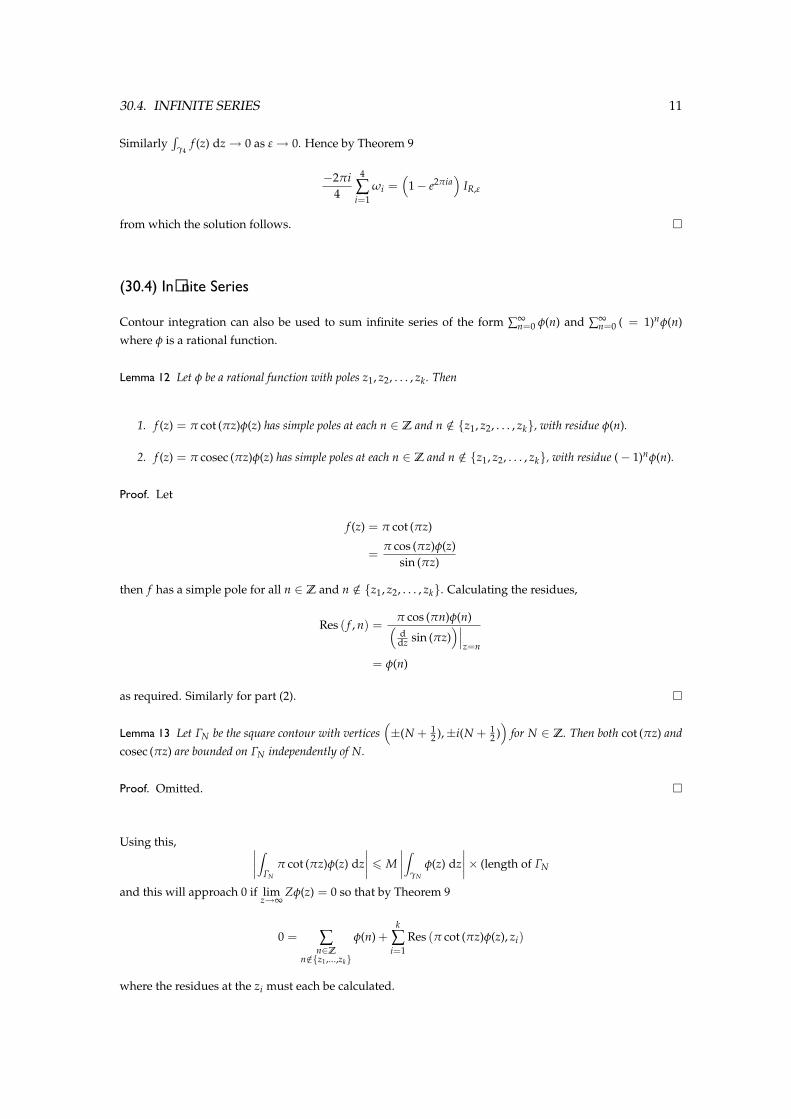
Similarly∫
γ4f (z) dz→ 0 as ε→ 0. Hence by Theorem 9
−2πi4
4
∑i=1
ωi =(
1− e2πia)
IR,ε
from which the solution follows. �
(30.4) Infinite Series
Contour integration can also be used to sum infinite series of the form ∑∞n=0 φ(n) and ∑∞
n=0 ( = 1)nφ(n)where φ is a rational function.
Lemma 12 Let φ be a rational function with poles z1, z2, . . . , zk. Then
1. f (z) = π cot (πz)φ(z) has simple poles at each n ∈ Z and n /∈ {z1, z2, . . . , zk}, with residue φ(n).
2. f (z) = π cosec (πz)φ(z) has simple poles at each n ∈ Z and n /∈ {z1, z2, . . . , zk}, with residue (− 1)nφ(n).
Proof. Let
f (z) = π cot (πz)
=π cos (πz)φ(z)
sin (πz)
then f has a simple pole for all n ∈ Z and n /∈ {z1, z2, . . . , zk}. Calculating the residues,
Res ( f , n) =π cos (πn)φ(n)(ddz sin (πz)
)∣∣∣z=n
= φ(n)
as required. Similarly for part (2). �
Lemma 13 Let ΓN be the square contour with vertices(±(N + 1
2 ),±i(N + 12 ))
for N ∈ Z. Then both cot (πz) andcosec (πz) are bounded on ΓN independently of N.
Proof. Omitted. �
Using this, ∣∣∣∣∫ΓN
π cot (πz)φ(z) dz∣∣∣∣ 6 M
∣∣∣∣∫γN
φ(z) dz∣∣∣∣× (length of ΓN
and this will approach 0 if limz→∞
Zφ(z) = 0 so that by Theorem 9
0 = ∑n∈Z
n/∈{z1,...,zk}
φ(n) +k
∑i=1
Res (π cot (πz)φ(z), zi)
where the residues at the zi must each be calculated.

12 CHAPTER 30. MSMYP1 FURTHER COMPLEX VARIABLE THEORY
(30.5) Conformal Mappings
(30.5.1) Angle Preserving Maps
A conformal map is a function of C → C which, roughly speaking, preserves local structure. However, ona larger scale such a map can produce dramatic changes. For example, mapping a circle to the upper halfplane.
Theorem 14 Let G be an open subset of C and let f : G → C be analytic on G. Let γ1 and γ2 be two contours in Gthat meet at a point z0. If f ′(z0) 6= 0 then f preserves the magnitude and direction of the angles between γ1 and γ2 atz0.
Proof. By re-scaling the interval upon which γ1 and γ2 are defined it may be assumed that γ1(t0) = z0 =γ2(t0). Also, by rotating the plane if necessary, it may be assumed that γ′2(t0) 6= 0. Now, the angle betweenγ1 and γ2 at z0 is the angle between the tangents. Hence
angle between γ1 and γ2 at z0 = arg (γ′1(t0))− arg (γ′2(t0)) = arg(
γ′1(t0)γ′2(t0)
)(15)
Similarly, the angle between the images of γ1 and γ2 under f at z0 is
arg(
( f ◦ γ)′1(t0)( f ◦ γ)′2(t0)
)= arg
(( f ′(γ1(t0))γ′1(t0)( f ′(γ2(t0))γ′2(t0)
)by applying the chain rule. But
f ′(γ1(t0) = f ′(z0) = f ′(γ2(t0) and f ′(z0) 6= 0
hence cancelling, this is the same as equation (15), and so the result is shown. �
This motivates the following definition.
Definition 16 Let G be an open subset of C and let f : G → C be analytic on G. f is conformal at z0 ∈ G if f ′(z0) 6= 0,and conformal on G if f ′(z0) 6= 0 ∀z0 ∈ G.
Some common and useful conformal maps are as follows.
• f (z) = z + a for a ∈ C. This is a translation in the direction−→0a .
• f (z) = zeiα for α ∈ R. This is an anticlockwise rotation through angle α about the origin.
• f (z) = kz for k ∈ R+. This is a dilation centred at the origin.
• f (z) = 1z . This is called an inversion, and it exchanges the inside and outside of the unit circle.
(30.5.2) Straight Lines, Circles, And The Mobius Transformation
Theorem 17 Let α, β ∈ C with α 6= β, and let λ ∈ R+. Then∣∣∣∣ z− α
z− β
∣∣∣∣ = λ
is the equation for a straight line or circle, and any straight line or circle has an equation of this form.
If λ = 1 then this is an equation for a straight line, otherwise the equation represents a circle.

30.5. CONFORMAL MAPPINGS 13
Definition 18 Let a, b, c, d ∈ C with ad− bc 6= 0 then the mapping
f : z 7→ az + bcz + d
is called the Mobius transformation.
Clearly translations, rotations, dilations, and inversions are all kinds of Mobius transformation. All Mobiustransformations are conformal maps, as
f ′(z) =ad− bc
(cz− d)2
Also, Mobius transformations are bijective, with inverse
f−1(w) =b− dwcw− a
Theorem 19 The image under a Mobius transformation of a straight line or circle is either a straight line or a circle.
Proof. Let L have equation z−αz−β = λ for some α 6= β and λ ∈ R+. Let f (z) = az+b
cz+d with ad− bc 6= 0 and letw = f (z) then
z =dw− ba− cw
substituting into the equation for L,
λ =
∣∣∣∣∣ dw−ba−cw − αdw−ba−cw − β
∣∣∣∣∣=∣∣∣∣ (dw− b)− α(a− cw)(dw− b)− β(a− cw)
∣∣∣∣=∣∣∣∣ (αc + d)w− (αa + b)(βc + d)w− (βa + b)
∣∣∣∣ (20)
which is in the form of a straight line or circle, or some degenerate case. There are 4 cases to consider.
• Suppose that αc + d = 0 = βc + d. But α 6= β, therefore c = 0 = d. But then ad − bc = 0, whichcontradicts that f is a Mobius transformation. Hence this case cannot occur.
• Suppose that αc + d 6= 0 6= βc + d then dividing through in equation (20),∣∣∣∣∣∣w−αa+bαc+d
w− βa+bβc+d
∣∣∣∣∣∣ = λ
∣∣∣∣ βc + dαc + d
∣∣∣∣∣∣∣∣w− f (α)w− f (β)
∣∣∣∣ = λ
∣∣∣∣ βc + dαc + d
∣∣∣∣which is the equation of a straight line or circle.
• Suppose that αc + d 6= 0 = βc + d then equation (20) gives
|w− f (α)| =∣∣∣∣ βa + b
αc + d
∣∣∣∣which is the equation of a circle.
• Suppose that αc + d = 0 6= βc + d then equation (20) gives
|w− f (β)| = 1λ
∣∣∣∣ αa + bβc + d
∣∣∣∣

14 CHAPTER 30. MSMYP1 FURTHER COMPLEX VARIABLE THEORY
which is the equation of a circle. �
The next obvious question is as to precisely which straight lines and circles can be sent where. A straightline or circle is uniquely determined by three points so, as the next theorem shows, any straight line or circlean in fact be sent to any other.
Theorem 21 For any pair of triples {z1, z2, z3} and {w1, w2, w3}with elements taken from C∪{∞} there is a uniqueMobius transformation f for which f (zi) = w1 for each of i = 1, 2, 3.
Proof. Choose w1 = 0, w2 = 1 and w3 = ∞. This can be done without loss of generality because Mobiustransformations are invertible, and so the transformation required by the theorem is then the compositiong−1 ◦ f where
z1f→0
g← w1
z2f→1
g← w2
z3f→∞
g← w3
Suppose then that f (z) = az+bcz+d , then it is required that
az1 + bcz1 + d
= 0az2 + bcz2 + d
= 1az3 + bcz3 + d
= ∞
By the requirement from z1, b = −az1.By the requirement from z3, d = −cz3.Hence
f (z) =az− az1bz− bz3
Now using the requirement from z2,
1 =ac
z2 − z1z2 − z3
which gives a value for ac and hence
f (z) =(
z2 − z3z2 − z1
)(z− z1z− z3
)Uniqueness follows since Mobius transformations are bijective. �
(30.5.3) Common Transformations
There are a number of common useful transformations. Moreover, these transformations can be combinedto produce more exotic transformations.
• To map the unit circle to the right half plane use f (z) = 1+z1−z .
• To map the right half plane to the positive quarter plane first apply the power map f (z) =√
z, thenrotate through an angle of π
4 by using the map g(z) = zei π4 . The power map f (z) = za for a ∈ R+
‘fans’ the plane, either ‘opening’ or ‘closing’ it.
• The exponential map f (z) = ez has numerous uses.
– To map the horizontal strip {z | a < Im z < b} to the wedge {z | a < arg z < b}.– To map the vertical strip {z | a < Re z < b} to the annulus {z | ea < |z| < eb}.
30.6. ANALYTIC FUNCTIONS 15
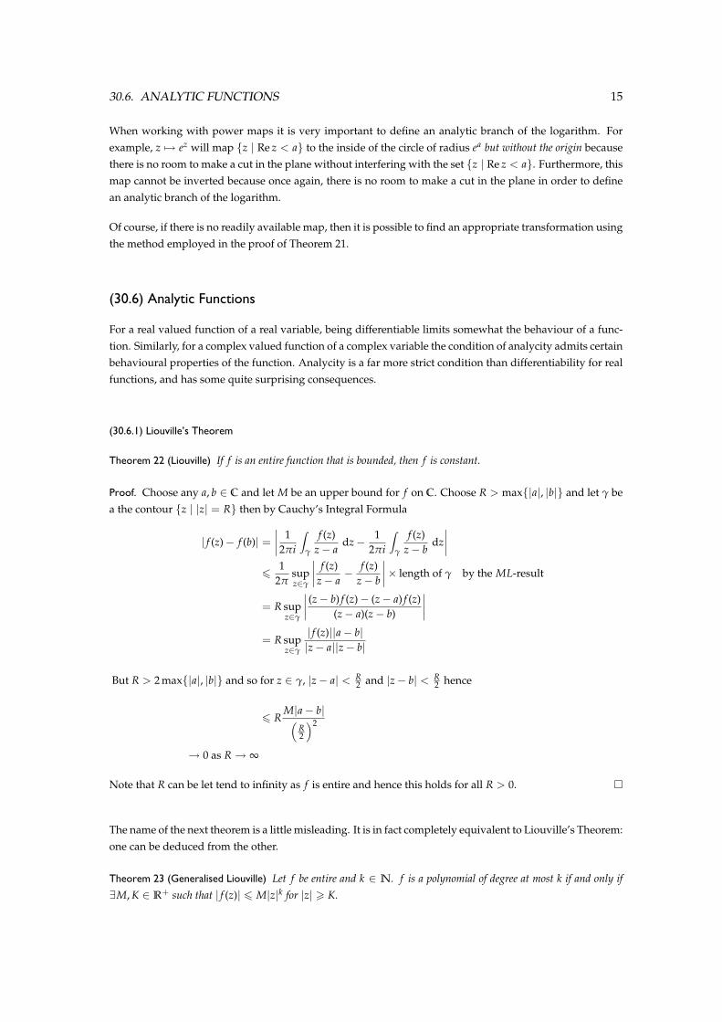
When working with power maps it is very important to define an analytic branch of the logarithm. Forexample, z 7→ ez will map {z | Re z < a} to the inside of the circle of radius ea but without the origin becausethere is no room to make a cut in the plane without interfering with the set {z | Re z < a}. Furthermore, thismap cannot be inverted because once again, there is no room to make a cut in the plane in order to definean analytic branch of the logarithm.
Of course, if there is no readily available map, then it is possible to find an appropriate transformation usingthe method employed in the proof of Theorem 21.
(30.6) Analytic Functions
For a real valued function of a real variable, being differentiable limits somewhat the behaviour of a func-tion. Similarly, for a complex valued function of a complex variable the condition of analycity admits certainbehavioural properties of the function. Analycity is a far more strict condition than differentiability for realfunctions, and has some quite surprising consequences.
(30.6.1) Liouville’s Theorem
Theorem 22 (Liouville) If f is an entire function that is bounded, then f is constant.
Proof. Choose any a, b ∈ C and let M be an upper bound for f on C. Choose R > max{|a|, |b|} and let γ bea the contour {z | |z| = R} then by Cauchy’s Integral Formula
| f (z)− f (b)| =∣∣∣∣ 12πi
∫γ
f (z)z− a
dz− 12πi
∫γ
f (z)z− b
dz∣∣∣∣
61
2πsupz∈γ
∣∣∣∣ f (z)z− a
− f (z)z− b
∣∣∣∣× length of γ by the ML-result
= R supz∈γ
∣∣∣∣ (z− b) f (z)− (z− a) f (z)(z− a)(z− b)
∣∣∣∣= R sup
z∈γ
| f (z)||a− b||z− a||z− b|
But R > 2 max{|a|, |b|} and so for z ∈ γ, |z− a| < R2 and |z− b| < R
2 hence
6 RM|a− b|(
R2
)2
→ 0 as R→ ∞
Note that R can be let tend to infinity as f is entire and hence this holds for all R > 0. �
The name of the next theorem is a little misleading. It is in fact completely equivalent to Liouville’s Theorem:one can be deduced from the other.
Theorem 23 (Generalised Liouville) Let f be entire and k ∈ N. f is a polynomial of degree at most k if and only if∃M, K ∈ R+ such that | f (z)| 6 M|z|k for |z| > K.
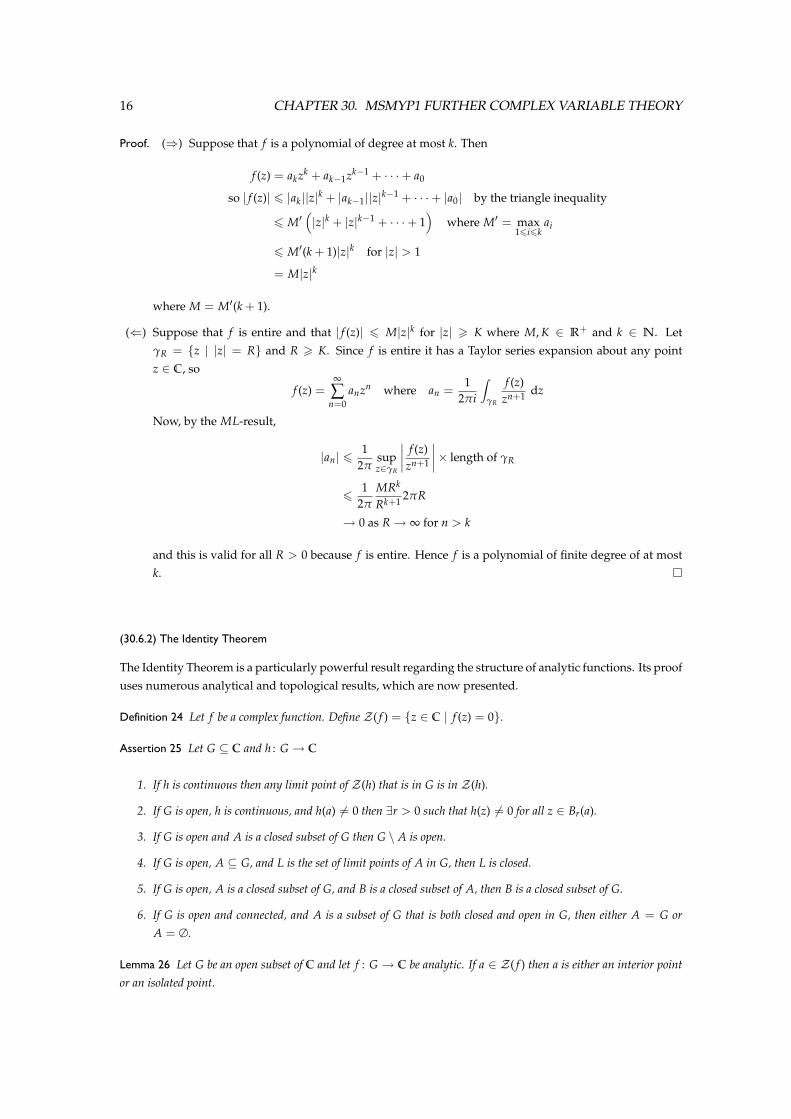
16 CHAPTER 30. MSMYP1 FURTHER COMPLEX VARIABLE THEORY
Proof. (⇒) Suppose that f is a polynomial of degree at most k. Then
f (z) = akzk + ak−1zk−1 + · · ·+ a0
so | f (z)| 6 |ak||z|k + |ak−1||z|k−1 + · · ·+ |a0| by the triangle inequality
6 M′(|z|k + |z|k−1 + · · ·+ 1
)where M′ = max
16i6kai
6 M′(k + 1)|z|k for |z| > 1
= M|z|k
where M = M′(k + 1).
(⇐) Suppose that f is entire and that | f (z)| 6 M|z|k for |z| > K where M, K ∈ R+ and k ∈ N. LetγR = {z | |z| = R} and R > K. Since f is entire it has a Taylor series expansion about any pointz ∈ C, so
f (z) =∞
∑n=0
anzn where an =1
2πi
∫γR
f (z)zn+1 dz
Now, by the ML-result,
|an| 61
2πsupz∈γR
∣∣∣∣ f (z)zn+1
∣∣∣∣× length of γR
61
2π
MRk
Rk+1 2πR
→ 0 as R→ ∞ for n > k
and this is valid for all R > 0 because f is entire. Hence f is a polynomial of finite degree of at mostk. �
(30.6.2) The Identity Theorem
The Identity Theorem is a particularly powerful result regarding the structure of analytic functions. Its proofuses numerous analytical and topological results, which are now presented.
Definition 24 Let f be a complex function. Define Z( f ) = {z ∈ C | f (z) = 0}.
Assertion 25 Let G ⊆ C and h : G → C
1. If h is continuous then any limit point of Z(h) that is in G is in Z(h).
2. If G is open, h is continuous, and h(a) 6= 0 then ∃r > 0 such that h(z) 6= 0 for all z ∈ Br(a).
3. If G is open and A is a closed subset of G then G \ A is open.
4. If G is open, A ⊆ G, and L is the set of limit points of A in G, then L is closed.
5. If G is open, A is a closed subset of G, and B is a closed subset of A, then B is a closed subset of G.
6. If G is open and connected, and A is a subset of G that is both closed and open in G, then either A = G orA = ∅.
Lemma 26 Let G be an open subset of C and let f : G → C be analytic. If a ∈ Z( f ) then a is either an interior pointor an isolated point.
30.6. ANALYTIC FUNCTIONS 17
Proof. Take any a ∈ Z( f ) then since f is analytic on G ∃r > 0 such that f has Taylor expansion
f (z) =∞
∑n=0
an(z− a)n ∀z ∈ Br(a)
Since f (a) = 0 it is immediate that a0 = 0. Further, either
1. an = 0 for all n ∈N∪ {0}, or
2. there must be some minimal m (m > 0 by the preceding statement) such that am 6= 0 but aj = 0 forj < m.
In the first case f (z) = 0 for all z ∈ Br(a) and hence Br(a) ⊆ Z(a), meaning that a is an interior point of Z(a).
In the second case,
f (a) = (z− a)m∞
∑n=0
an+m(z− a)n ∀z ∈ Br(a)
Let g(z) = ∑∞n=0 an+m(z− a)n then g is analytic on Br(a) and therefore is continuous. Also, g(a) = am 6= 0.
But then ∃s > 0 with s 6 r such that g(z) 6= 0 for all z ∈ Bs(a) \ {a}. But f (z) = (z− a)mg(z) which is thenalso non-zero on Bs(a) \ {a} and hence Z( f )∩ Bs(a) = {a} i.e., a is an isolated point of Z f . �
Corollary 27 If an analytic function f has an isolated zero at a then the zero is of finite multiplicity and f (z) =(z− a)mg(a) where g(z) 6= 0 for z ∈ Bs(a) and g is analytic on G.
Proof. As in case 2 in the proof of Lemma 26 define g by
g(z) =
am if z = af (z)
(z−a)m if z 6= afor z ∈ Bs(a)
then g is analytic (including at a), and is non-zero in Bs(a). �
Theorem 28 (Identity) Let G be an open and connected subset of C, and let f : G → C be analytic. If Z( f ) has a limitpoint in G, then f is identically zero.
Proof. Let L be the set of limit points of Z( f ) that lie in G.By Assertion 25 L ⊆ Z( f ) and is a closed subset of Z( f ) which is a closed subset of G. Therefore L is a closedsubset of G.
Take any z0 ∈ L, then z0 ∈ Z( f ). Since z0 ∈ L it is not an isolated point of Z( f ) and hence by Lemma 26 z0
is an interior point of Z( f ). But then ∃r > 0 such that Br(z0) ⊆ Z( f ). Now, every point of Br(z0) is a limitpoint of Br(z0) and therefore Br(z0) ⊆ L, meaning that L is an open subset of G.
Hence L is both open and closed in G which is open and connected. Hence either L = G or L = ∅.
Now, by hypothesis Z( f ) has a limit point in G, therefore L 6= ∅. Hence L = G. But L ⊆ Z( f ) and thereforeZ( f ) = G, i.e., f is identically zero on G. �
18 CHAPTER 30. MSMYP1 FURTHER COMPLEX VARIABLE THEORY