52

CHAPTER 3

WAVELET AND CURVELET BASED IMAGE

COMPRESSION WITH DEAD ZONE QUANTIZATION

3.1 INTRODUCTION

An image file contains huge amounts of information that

requires high storage space, large transmission bandwidths and long

transmission times. So it is useful to compress the image by storing only

the required information to reconstruct the original image. An image can be

considered as a matrix of pixel or intensity values. In order to compress an

image redundancies must be evaluated, for example, several areas where

there is small change or there is no change among pixel values Hariom

Yadav & Hitesh Gupta (2013). So the images having the consistent color

with larger areas will have large redundancies, and on the other hand an

image having more changes in color by means of less redundant becomes

more difficult to compress.

Wavelet analysis can be used to separate the information of an

image into determination and aspect subsignals Karen Lees (2002).

The estimation of subsignal shows the universal tendency of pixel values

and these subsignals shows that results of the information or changes in the

images according to vertical, horizontal and diagonal regions. If the result

becomes a small value it can automatically set to zero without considerably

altering the image. The value which is set to zero is called as threshold

53

value. More number of zeroes in the result show that the compression

achieves better value. Energy retained is defined as the amount of

information retained by an image after compression and decompression

and it is proportional to the sum of the squares of the pixel values in the

image. If there is no change in the image, the energy retained achieves 100

% result. This type of compression is known as lossless; Lossless

compression result the reconstruction of image that will produce exact

image before and after compression. Reconstruction of the images is exact

when the threshold value is zero. If any changes made in image, the energy

retrained will be lost and it is known as lossy compression. During the

compression process, initially of zeros and the energy maintenance

motivation is as high as probable. However, as more zeros are obtained,

more energy is lost, so stability among the two requirements are to be

established.

3.2 WAVELET TRANSFORMATION IN IMAGE

PROCESSING

Wavelet transforms and further multi-scale examination

functions have been secondary for compacted signal and image

representation in de-noising, compression and feature detection processing

problems for concerning 20 years (Ebrahimi & Pazirandeh 2011). Various

research works have demonstrated that space-frequency and space-scale

expansions with this family of study functions provided an extremely well-

organized structure for signal or image data.

The wavelet transform function offers suitable design.

Beginning with selection, spatial-frequency tiling and a variety of wavelet

threshold strategies result optimized output for a processing application,

data individuality and feature of importance. Fast accomplishment of

54

wavelet transforms by means of a filter-bank structure allows real time

processing capacity. As an alternative of trying to restore image processing

techniques, wavelet transforms recommend a well-organized

demonstration of the signal, finely tuned to its built-in property.

By combining such demonstration with simple processing techniques in the

transform, multi-scale examination can achieve remarkable performance

for several image processing problems.

Wavelet-based compression is an individual category of

transform-based compression. Universal transform-based compression

system is shown in Figure 3.1. For wavelet-based compression, a wavelet

transform and its inverse are used for the transform and inverse transform,

correspondingly (James S Walker 2002).

(a) Compression process

(b) Decompression process

Figure 3.1 Transform based compression

The compression schema starts by transforming the image from

data space to wavelet space. This process can be done in several ways.

By applying the data into bi-dimensional transform matrix and in the

Image Transform Encode Transform

values

Compressed Image

Compressed Image

Decode Transform

values

Inverse Transform

Image

55

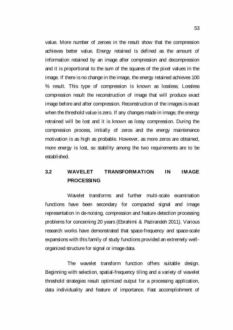
resulting image the coe cients were obtained and grouped into four zones

shown in Figure 3.2, where H symbolizes high frequency data and L

symbolizes low frequency data

Figure 3.2 Discrete wavelet transform frequency quadrants

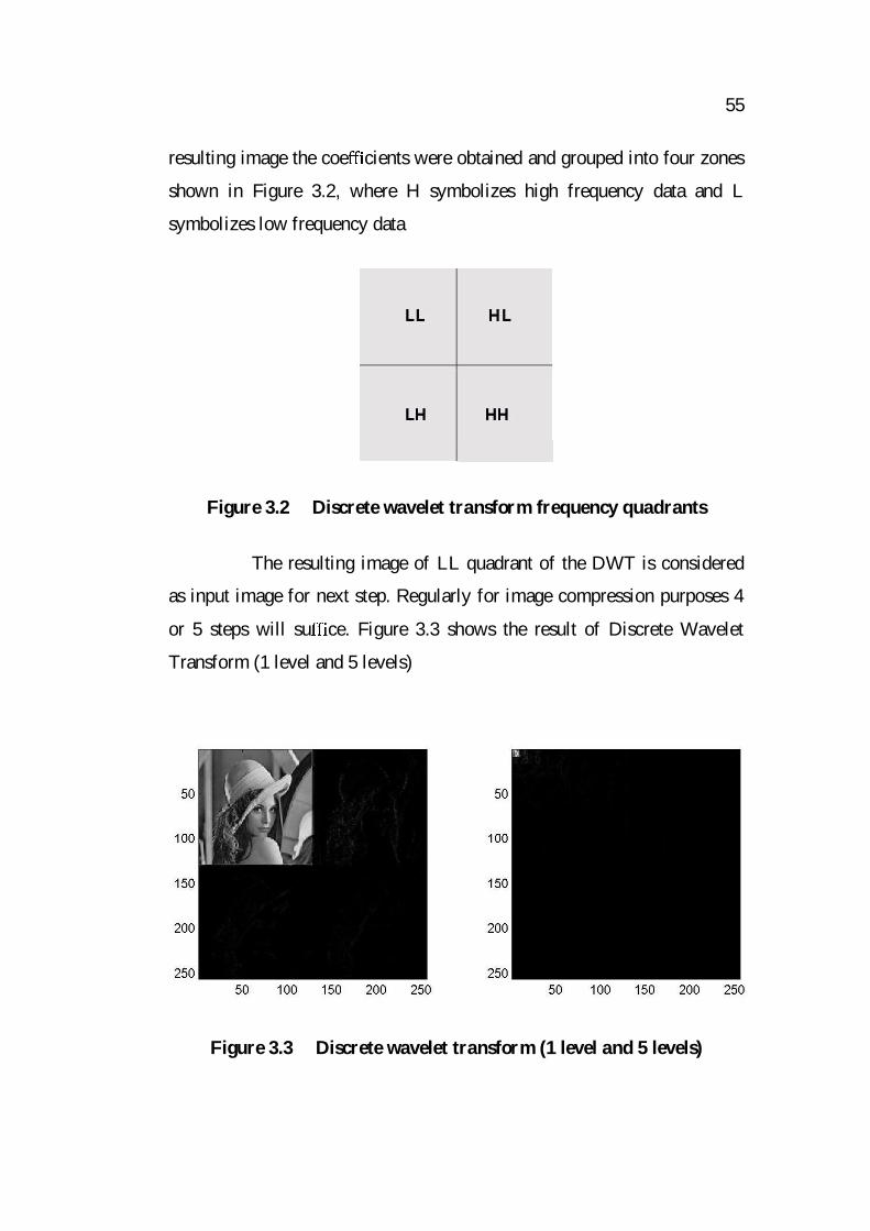
The resulting image of LL quadrant of the DWT is considered

as input image for next step. Regularly for image compression purposes 4

or 5 steps will su ce. Figure 3.3 shows the result of Discrete Wavelet

Transform (1 level and 5 levels)

Figure 3.3 Discrete wavelet transform (1 level and 5 levels)

56

DWT of 5 levels data is also obtainable in a mesh form to

visualize different improved intensities of the coe cients. The majority of

the DWT intensities are situated in the upper of LL quadrant.

3.3 DISCRETE WAVELET TRANSFORM IN IMAGE

COMPRESSION

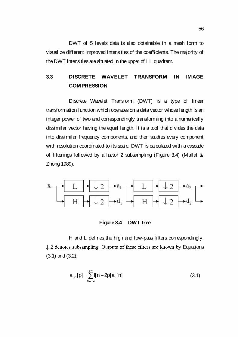
Discrete Wavelet Transform (DWT) is a type of linear

transformation function which operates on a data vector whose length is an

integer power of two and correspondingly transforming into a numerically

dissimilar vector having the equal length. It is a tool that divides the data

into dissimilar frequency components, and then studies every component

with resolution coordinated to its scale. DWT is calculated with a cascade

of filterings followed by a factor 2 subsampling (Figure 3.4) (Mallat &

Zhong 1989).

Figure 3.4 DWT tree

H and L defines the high and low-pass filters correspondingly,

Equations

(3.1) and (3.2).

nj1j ]n[a]p2n[l]p[a (3.1)

57

nj1j ]n[a]p2n[h]p[d (3.2)

Elements aj are used for next step (scale) of the transform and

basics dj, called wavelet coefficients, establish output of the transform. l[n]

and h[n] are coefficients of low and high-pas filters correspondingly.

One can assume that on scale j+1 there is simply half from numeral of a

and d elements on scale j. This causes that DWT can be complete until

simply two aj elements stay behind in the analyzed signal and it’s called as

scaling function coefficients.

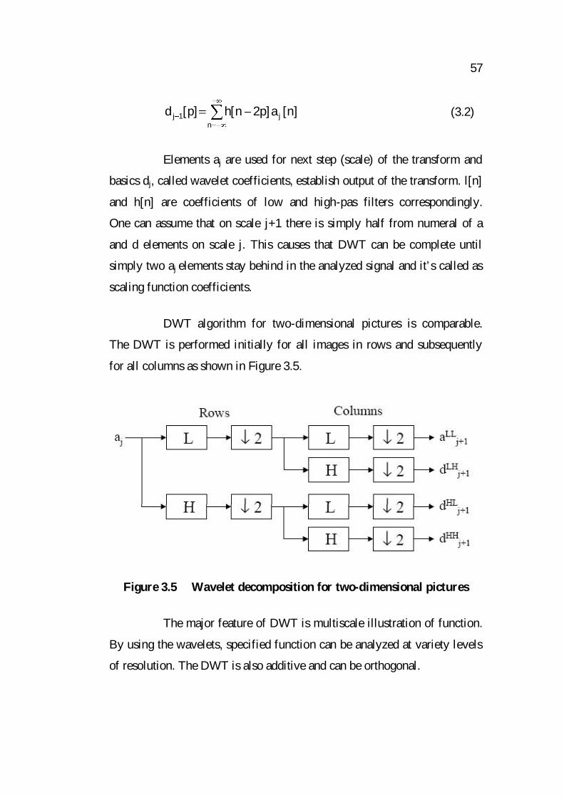
DWT algorithm for two-dimensional pictures is comparable.

The DWT is performed initially for all images in rows and subsequently

for all columns as shown in Figure 3.5.

Figure 3.5 Wavelet decomposition for two-dimensional pictures

The major feature of DWT is multiscale illustration of function.

By using the wavelets, specified function can be analyzed at variety levels

of resolution. The DWT is also additive and can be orthogonal.

58

Wavelets appear to be efficient for analysis of textures recorded

with diverse resolution. It is very significant problem in NMR imaging,

since high-resolution images necessitate long time of attainment.

This causes a raise of artifacts caused by patient actions, which be

supposed to be avoided. There is a probability that the proposed approach

will offer a tool for speedy, small resolution NMR medical diagnostic.

3.3.1 Significant Properties of Wavelets

The key transform used in denoising is by using wavelets Tim

Park (2011). To assist stimulate and to employ wavelets in universal and

specially for de-noising, describe several of the properties which have

made wavelets so useful in several different areas. Wavelet analysis has

more advantages than Fourier analysis.This in several ways comes down to

the detail that Fourier analysis describes global properties of the data and,

as such, is not a good illustration of local properties.

3.3.2 Significance of Wavelets in Image Compression

Loss of several information is inevitable for image compression

as discussed in previous section. Amongst all of the mentioned above lossy

compression methods, vector quantization needs numerous computational

resources for large vectors; fractal compression is a time consuming task

for coding; analytical coding has inferior compression ratio and poorer

reconstructed image superiority than transformation based coding.

So, transform based compression methods are well suited methods for

image compression.

For transform based compression, JPEG image compression

schemes based on DCT (Discrete Cosine Transform) have more

59

advantages such as easy, enhanced performance results, and for

implementation. Since the input image is blocked separately, correlation

among individual block boundaries cannot be eliminated. This results in

acceptable and annoying blocking artifacts mainly at low bit rates.

Over the past years, wavelet transform function has been used

for signal processing mainly, in image compression. Wavelet-based

schemes achieve greater results than other coding schemes based on DCT.

Since there is no need of blocking the input image, their base function

includes variable length.

3.4 AN OVERVIEW OF CURVLET TRANSFORM

Wavelet transform is regarded as a better selection than Fourier

transform due to its ability to restrict in frequency and time at the same

time Kiruthika & Thirumaraiselvi (2012). This approach is extremely

useful while examining time-varying phenomenon in normal images

(Burrus et al 1998). The fine data content in images is regularly found in

the high frequencies whereas the coarse information content is present in

the low frequencies. WT exploits its multi-resolution capability to

decompose the image into several frequency bands. The WT suffers from

the following issues:

2-D line singularities: Piecewise smooth signals are equivalent

to images having one dimentional Singularities. In 2-D image, the smooth

areas are partitioned by edges, whereas edges are discontinuous across.

They are classically smooth curves.

Lack of shift invariance: This occurs due to the down sampling

procedure at every stage. When the input signal is shifted a small, the

60

wavelet coefficients amplitude differs mostly (Kingsbury 2001).

Lack of directional selectivity: As the DWT filters are real and

distinguishable the DWT cannot discriminate amongst the opposite

diagonal directions (Kingsbury 2001).

The above said issues can be overcome by the development of

well-organized transformations. In order to study local line or curve

singularities, ridgelet transform can be applied to the sub-images (Siva

Nagi Reddy et al 2012). The second generation of curvelet transforms deal

with the image boundaries by mirror expansion. The second- generation

curvelet transform have been observed to be extremely effectual for

numerous applications in image processing. So, this thesis work uses

approach uses curvelet transformation.

Curvelets are a non adaptive method for multi-scale object

demonstration. Being an expansion of the wavelet concepts, they are

appropriately used in related fields, specifically in image processing and

scientific computing.

Wavelets specify the by means of a basis along with the

representation of location and spatial frequency. Directional wavelet

transforms using basis functions are restricted in orientation of 2D and 3D

signals. Curvelet transform varies from traditional directional wavelet

transforms based on the degree of localization in orientation. Specifically

fine-scale base functions are lengthy ridges; the shape of these function

ranges from j is 2-j by 2-j/2 so the fine-scale basis are thin ridges with an

exactly single-minded direction.

61

Curvelets are suitable for representation of basic images which

are smooth and different from singularities all along with smooth curves,

where the smooth curves enclose bordered curvature with images having

less length scale. This type of property used for cartoons, geometrical

diagrams, and multimedia application such as text files. Zooming the

images with the edges they enclose appear, gradually more instantly.

Curvelet methods use this property, by defining the upper resolution

curvelets in the direction of skinnier to lower resolution curvelets values.

However, normal image do not follow this property; they contain details at

each and every scale. So, for the natural images, it is preferable to make

use of some sort of directional wavelet transform for which wavelets have

the similar characteristic ratio at every scale. While the image is of the

correct kind, curvelets give an illustration that is significantly sparser than

other wavelet transforms. This can be quantified by taking into

consideration, the best estimation of a geometrical test image that can be

represented using n wavelets and analyzing the estimation error as a

function of n. For a Fourier transform, the error decreases only as 2/1n1 .

For a wide range of wavelet transforms, together with both directional and

non-directional variants, the error decreases as n1O . The additional

assumption with curvelet transform allows it to achieve the value of

2

3

n))n(log(O .

Efficient numerical algorithms are used for computing the

curvelet transform of discrete data. Computational cost of a curvelet

transform is approximately 10 - 20 times higher than the Fast Fourier

Transform (FFT) and has the similar complexity of O(n2log(n)) for an

62

image of dimension n x n.

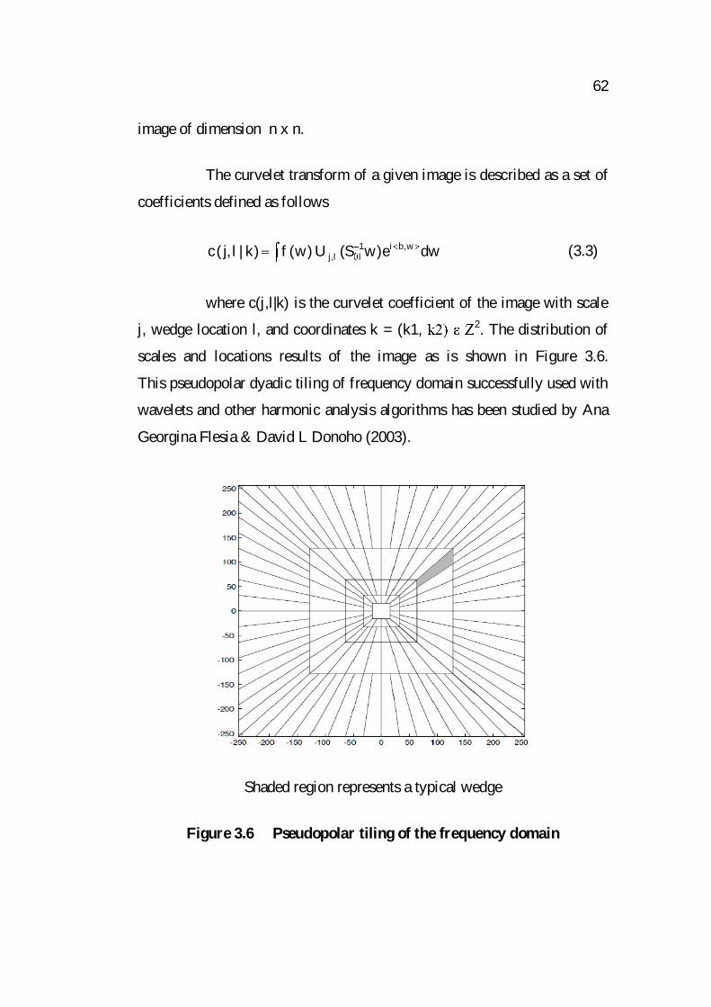
The curvelet transform of a given image is described as a set of

coefficients defined as follows

dwe)wS(U)w(f)k|l,j(c w,bi1ll,j (3.3)

where c(j,l|k) is the curvelet coefficient of the image with scale

j, wedge location l, and coordinates k = (k1, 2. The distribution of

scales and locations results of the image as is shown in Figure 3.6.

This pseudopolar dyadic tiling of frequency domain successfully used with

wavelets and other harmonic analysis algorithms has been studied by Ana

Georgina Flesia & David L Donoho (2003).

Shaded region represents a typical wedge

Figure 3.6 Pseudopolar tiling of the frequency domain

63

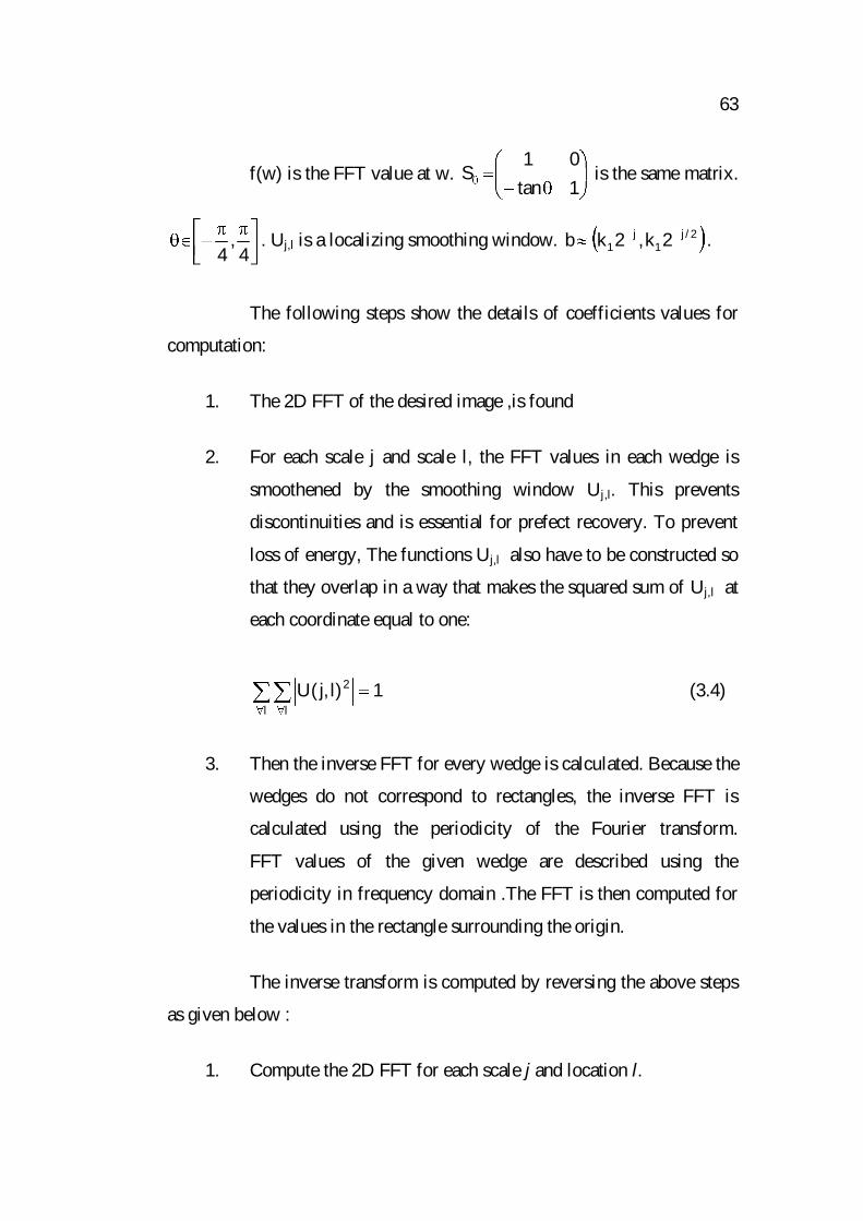
f(w) is the FFT value at w. 1tan01

S is the same matrix.

4,

4. Uj,l is a localizing smoothing window. 2/j

1j

1 2k,2kb .

The following steps show the details of coefficients values for

computation:

1. The 2D FFT of the desired image ,is found

2. For each scale j and scale l, the FFT values in each wedge is

smoothened by the smoothing window Uj,l. This prevents

discontinuities and is essential for prefect recovery. To prevent

loss of energy, The functions Uj,l also have to be constructed so

that they overlap in a way that makes the squared sum of Uj,l at

each coordinate equal to one:

l l

2 1)l,j(U (3.4)

3. Then the inverse FFT for every wedge is calculated. Because the

wedges do not correspond to rectangles, the inverse FFT is

calculated using the periodicity of the Fourier transform.

FFT values of the given wedge are described using the

periodicity in frequency domain .The FFT is then computed for

the values in the rectangle surrounding the origin.

The inverse transform is computed by reversing the above steps

as given below :

1. Compute the 2D FFT for each scale j and location l.

64

2. Multiply each one scale/location by the correspondent

smoothing window. The smoothing window needs to be

‘wrapped’ to correspond to the novel distribution of frequency

values are computed by step 3 in the forward transform.

3. The frequency values are mapped as group ‘unwrapped’ to their

unique scale/wedge location. Then perform 2D inverse FFT, to

acquire the original image back again.

Substitute to the wrapping approach, in computing the FFT for

curvelet wedges, is to turn the coordinate system by aligning the

orientation of each wedge locations. In this case,

dwe)wS(U)w(f)k|l,j(c w,bi1ll,j (3.5)

These types of curvelet based implementation are done through

online. The results presented in this thesis work are relevant to either one

of them. Due to high computational complexity and to avoid interpolation

artifacts in this work wrapper based implementation is done from

Figure 3.7, it is clear that the coarsest level (j = 1) is not directional.

Its effect is similar to a low pass filter. The corresponding coefficient

values represent the smoothest areas in the image. Outer finest level is

developed using either directional or non-directional related curvelets.

Directional curvelets are high computational cost with enhanced better

results. In this work focus is made on directional curvelets. The ratio of the

new size to the old one is fixed at 1.3. The number of scales J is determined

by the size of the input image. The number of wedges per scale rises from

the coarsest scale to the finest that is equal to 22j where j = 1,2...J.

Although, that values of curvelet coefficients are entirely estimated by the

frequency content, tiling of the frequency space takes the similar dyadic

65

approach with frequently fixed parameters. Using these adaption divisions

to match to the frequency content in the image will generate better

performance results

3.5 QUANTIZATION

Quantization is a lossy compression technique in image

processing. It is achieved by compressing the series of values to a single

quantum value. The number of distinct symbols in a known stream is

reduced and the stream becomes further compressible. Precise applications

contain DCT data quantization in JPEG and DWT data quantization

in JPEG 2000. The quantizer has an important impact on the amount of

compression obtained and loss, subject to a lossy compression system.

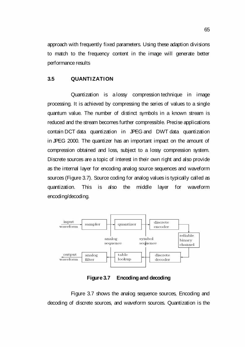
Discrete sources are a topic of interest in their own right and also provide

as the internal layer for encoding analog source sequences and waveform

sources (Figure 3.7). Source coding for analog values is typically called as

quantization. This is also the middle layer for waveform

encoding/decoding.

Figure 3.7 Encoding and decoding

Figure 3.7 shows the analog sequence sources, Encoding and

decoding of discrete sources, and waveform sources. Quantization is the

66

middle layer process and should be understood before entering into the

outer layer, which deals with waveform sources.

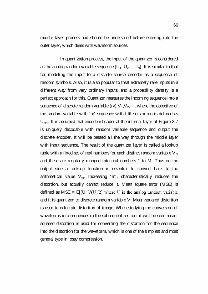
In quantization process, the input of the quantizer is considered

as the analog random variable sequence (U1, U2… UN). It is similar to that

for modeling the input to a discrete source encoder as a sequence of

random symbols. Also, it is also popular to treat extremely rare inputs in a

different way from very ordinary inputs, and a probability density is a

perfect approach for this. Quantizer measures the incoming sequence into a

sequence of discrete random variable (rv) V1,V2, ···, where the objective of

the random variable with ‘m’ sequence with little distortion is defined as

Umm. It is assumed that encoder/decoder at the internal layer of Figure 3.7

is uniquely decodable with random variable sequence and output the

discrete encoder. It will be passed all the way through the middle layer

with input sequence. The result of the quantizer layer is called a lookup

table with a fixed set of real numbers for each distinct random variable Vm

and these are regularly mapped into real numbers 1 to M. Thus on the

output side a look-up function is essential to convert back to the

arithmetical value Vm. Increasing ‘m’, characteristically reduces the

distortion, but actually cannot reduce it. Mean square error (MSE) is

defined as MSE = E[(U

and it is quantized to discrete random variable V. Mean-squared distortion

is used to calculate distortion of image. When studying the conversion of

waveforms into sequences in the subsequent section, it will be seen mean-

squared distortion is used for converting the distortion for the sequence

into the distortion for the waveform, which is one of the simplest and most

general type in lossy compression.

67

3.5.1 Vector Quantization

Image compression can be categorized into two types namely as

Lossy Compression and Lossless Compression. In lossless compression,

the unique image can be entirely recovered from the compressed image.

Lossless Compression is useful for applications with precise requirements

such as medical imaging, whereas lossy compression is mainly suitable for

natural images similar to photos in applications wherever minor loss is

acceptable to achieve a significant reduce in bit rate.

Vector Quantization (VQ) is a type of quantization technique in

signal processing which uses the probability density functions (pdf) by the

circulation of prototype vectors. It was originally used for data

compression. It works by partitioning a large set of vectors into groups

having approximately the similar number of vectors closest to them. Each

group of vector is represented as centroid value in k-means and other

clustering algorithm also. Probability density function is powerful,

particularly for identifying the density level of large and high-dimensioned

data. Since data points are represented by the index of their closest

centroid, normal data contain low error and exceptional data high error.

Hence it is appropriate to consider this for lossy data compression. It can

also be used for lossy data correction and density estimation.

3.5.2 Image Compression based on Vector Quantization

Vector Quantization (VQ) coding is an image compressing

scheme (Chin-chen et al 2013). In this method, an index table for the

original image is generated. The receiver can restructure the image simply

by the index table and the pre-training VQ codebook. VQ is unique of

lossy compression techniques. For a given image which consists of

68

256×256 pixels, the superiority of reconstructing is an image is getting

27 dB to 30 dB where the codebook size is 256. In order to get better

performance of the quantization, in this work dead zone quantization

technique is used.

3.6 ENCODING APPROACHES

In lossless compression techniques, the input image can be

easily recovered from the compressed image. These are also called

noiseless image, because it is performed without adding noise value in

image. It is also well-known as entropy coding because it uses

statistics/decomposition approaches to remove/reduce redundancy.

Lossless compression is used only for a small number of applications with

stringent necessities such as medical imaging.

3.6.1 Set Partitioning In Hierarchical Trees (SPIHT)

There is a parent-child association among the wavelet

coefficients. Every coefficient at a known scale is associated to a set of

coefficients at the subsequently finer scale of similar orientation.

The wavelet coefficient in the coarse range is called parent. Every parent

has four children at the next finer range of similar direction. It is based on

the theory of parent-child association among the wavelet coefficients.

Encoding step consists of two quantization passes namely sorting pass and

the refinement pass. The algorithm maintains the data structure with three

linked lists the LSP, LIP and the LIS.

The algorithm maintains three linked list to keep important and

unimportant pixels and their corresponding sets:

LSP: list of significant pixels

69

LIP: list of insignificant pixels

LIS: list of insignificant sets

These three lists are used to keep way of the original image

throughout encoding process. Throughout sorting pass, new important

entries in LIP and LIS are identified and their corresponding signs are

coded. In every refinement pass, every coefficient in LSP apart from the

ones added in the previous sorting pass in refined. The image is

reconstructed by the quantization procedure; the quantization step halves

the threshold every time. The encoding procedure stops up when a target

bit rate or threshold or quality condition is reached.

Roots of the all spatial orientation trees are

O(i,j): Set of offspring of the coefficient

(i,j) = {(2i,2j),(2i,2j+1),(2i+1,2j),(2i+1,2j+1)}, except (i,j) is in

LL; when coefficient (i,j) is in LL subband,

O(i,j) is defined as: O(i,j) = {(i,j+wLL), (i+hLL,j),

(i+hLL,j+wLL)}, where wLL and hLL is the width and height

of the LL subband, respectively.

D(i,j): Set of all descendants of the coefficient(i,j), L(i,j): D(i,j) – O(i,j)

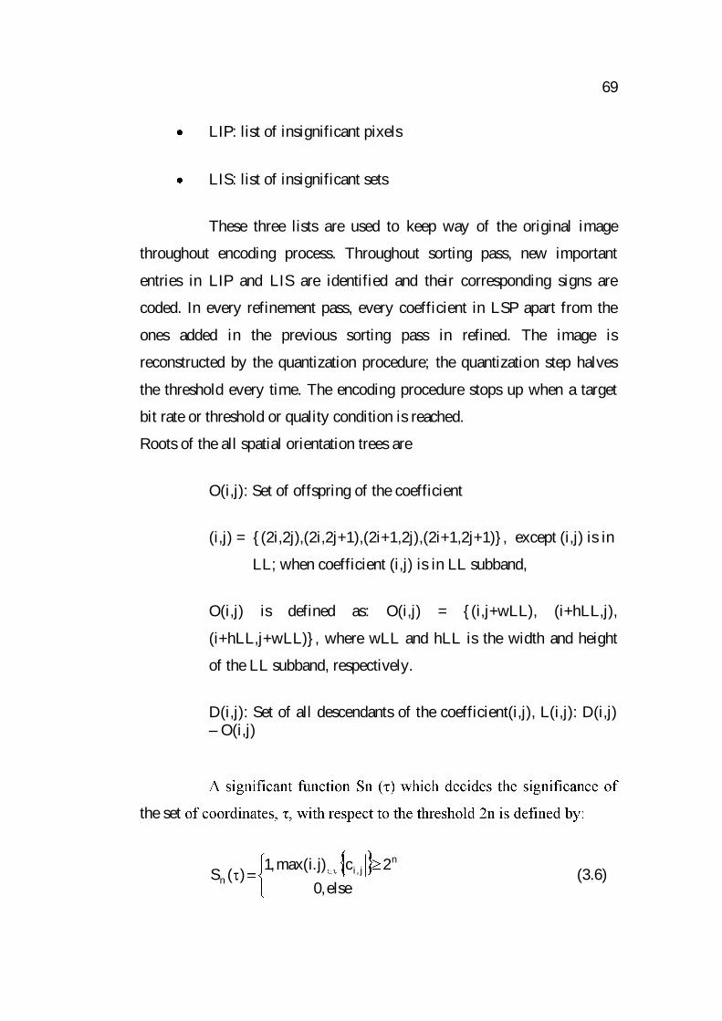
the set

else,02c)j.imax(,1)(S

nj,i

n (3.6)

70

At the initialization stage, LSP is set to empty list. LIP values

are initialized with all coefficients in the maximum level of the wavelet LL

subband. LIS values are initialized with all the coefficients in the

maximum level of the wavelet LL subband with descendents. During the

sorting pass, the algorithm primary traverses during the LIP, testing the

magnitude of its fundamentals beside the present threshold and

representing their significance by 0 or 1. Each time when a coefficient is

found important, its sign is converted and it is moved to LSP. The

algorithm then examines the LIS and performs a magnitude on all

coefficients of set. If a particular tree/set is established to be important, it is

partitioned into its subsets and tested for significance. Else a single bit is

added to the bit stream to point out an unimportant set. After every sorting

pass is completed SPIHT outputs modification bits at the present level of

bit which have been moved to LSP list. The results of SPHIT output the

refinement bits that decrease highest error. This process continues by

decreasing current threshold by factor of two until desired bit rate is

achieved. SPIHT is an embedded coding technique. In embedded coding

algorithms, encoding of the similar signal at lower bit rate is embedded at

the start of the bit stream for the target bit rate. Effectively, bits are ordered

in importance. This type of coding is particularly helpful for continuous

transmission by means of an embedded code; where an encoder can

conclude the encoding procedure at any situation.

SPIHT algorithm is based on the following concepts (Said &

Perlman 1996, Kim & Pearlman 1997)

1. Ordered bit plane progressive transmission.

2. Set partitioning sorting algorithm.

71

3. Spatial orientation trees.

SPIHT keeps each state with three lists namely LIP, LSP and

LIS. Each list stores pixel values. Insignificant pixels are stored by LIP,

significant pixel values are stored by LSP and insignificant pixel values are

stored by LIS. At the start, LSP is empty, LIP keeps all coefficients values

in lower sub band, and LIS keeps the complete tree roots which are at the

lower sub band. SPHIT algorithm can be performed in two pass.

The primary pass is the sorting pass. It initially browses the LIP and move

towards entire considerable coefficients to LSP and outputs its sign. Then it

browses LIS executing the information and subsequent the partitioning

sorting algorithms.

The subsequent pass is the refining pass. It searches the

coefficients in LSP and results a single bit only based on the present

threshold. After the two passes are completed, the threshold is separated by

2 and the encoder process these two passes over again. This process is

recursively applied until the output bits reach the preferred number.

3.6.2 Use of Dead Zone Quantization with Curvelet

After the curvelet transform, all the subbands are quantized in

lossy compression to reduce the precision of the subbands to assist in

achieving compression. Quantization of curvelet subbands is one of the

major sources of data/information loss in the encoder. Quantization is done

by uniform scalar quantization with dead-zone (Soo-Chang Pei & Ching-

Min Cheng (1995). In dead-zone scalar quantizer the step size is defined as

b, the width of the dead-zone is defined as 2 b as shown in Figure 3.8.

It supports split quantization step sizes for every subband. The quantization

step size ( b) for a subband (b) is determined based on the active series of

72

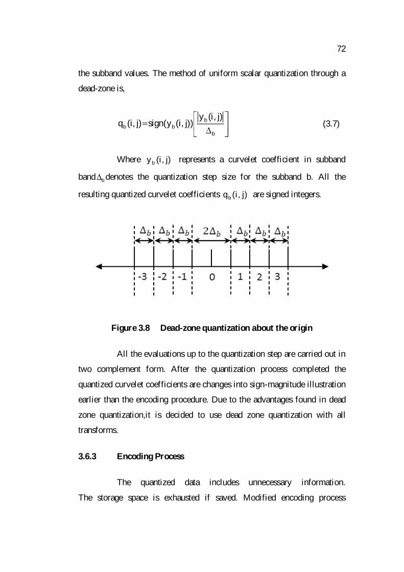
the subband values. The method of uniform scalar quantization through a

dead-zone is,

b

bbb

)j,i(y))j,i(y(sign)j,i(q (3.7)

Where )j,i(y b represents a curvelet coefficient in subband

band b denotes the quantization step size for the subband b. All the

resulting quantized curvelet coefficients )j,i(q b are signed integers.

Figure 3.8 Dead-zone quantization about the origin

All the evaluations up to the quantization step are carried out in

two complement form. After the quantization process completed the

quantized curvelet coefficients are changes into sign-magnitude illustration

earlier than the encoding procedure. Due to the advantages found in dead

zone quantization,it is decided to use dead zone quantization with all

transforms.

3.6.3 Encoding Process

The quantized data includes unnecessary information.

The storage space is exhausted if saved. Modified encoding process

73

overcomes this problem. It is an illustration of a lossless data compression

approach that offers a way of eliminating the unnecessary quantized

information without any loss of information.

A. The Zero Shifting

The method of zero shifting is a straightforward and easy-to-

implement technique which conserves the embedded features of the SPIHT

coding. By downward scaling of the pixel values by 2(N-1), N being the

number of bits of the original pixel, the spatial field magnitude becomes

bipolar ranging from (-2(N-1)) to (+2(N-1)-1), nearly equal to the half of

the maximum absolute spatial value.

In the transform field, the wavelet lifting system results the high

pass subband by measuring the weighted differences between of pixel

values after completion of prediction. Likewise, the low pass subband is

decreased by computing the weighted average of pixel values after the

completion of updating step. This low pass subband is decomposed

iteratively for every level of decomposition ending with one lowest

frequency band, the rest being high frequency bands.

SPIHT coding is one of the types of bit plane coding

techniques.In this method, the largest number bit plane is determined by

the maximum absolute assessment of the altered coefficients. As the

maximum coefficient reduces using the method of zero shifting, it takes

less time for both encoding and decoding. Further, the lower section of the

complete image in the spatial domain values from 1N2p0 j,i are

shifted to a higher exact range in the bipolar sense. The lower image values

get detailed information pertaining to the limits, ends, etc.

These coefficients become important at a larger threshold value and hence

74

are obtained in the bit level surface progressive transmission of the SPIHT

bit stream. Since SPIHT algorithm forever encodes a sign bit for significant

coefficients, no other additional bit is needed for being bipolar. By

stopping the decoding process still at a lower bit rate, the quality improves,

together individually and independently, due to the inclusion of some point

of information at that rate.

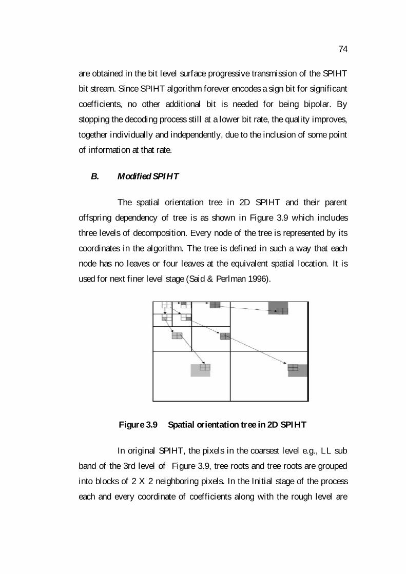
B. Modified SPIHT

The spatial orientation tree in 2D SPIHT and their parent

offspring dependency of tree is as shown in Figure 3.9 which includes

three levels of decomposition. Every node of the tree is represented by its

coordinates in the algorithm. The tree is defined in such a way that each

node has no leaves or four leaves at the equivalent spatial location. It is

used for next finer level stage (Said & Perlman 1996).

Figure 3.9 Spatial orientation tree in 2D SPIHT

In original SPIHT, the pixels in the coarsest level e.g., LL sub

band of the 3rd level of Figure 3.9, tree roots and tree roots are grouped

into blocks of 2 X 2 neighboring pixels. In the Initial stage of the process

each and every coordinate of coefficients along with the rough level are

75

placed into the LIP listing and the coordinates of coefficients having only

descendants are placed into LIS list as D-type sets. Proposed work can be

done by making modification in initial stage of the process of the SPIHT

algorithm with the principle of null shifting value as follows: in the

decomposition level the coarsest level of LL subband which consists of

only one pixel level and set LIS list with all coordinates of the coarsest

level which is also single pixel level, else initialize the LIS list through LL

subband at the same time as of the LIP list with every coordinates.

Consequently, sorting the values in LIS list, SPIHT algorithm first tests the

band values that corresponding to LH, HL, and HH for lowest subband.

For each root in LL, it compares the utmost value among the other three

bands at the same time in spatial orientation and sorts it in the output bit

stream. Once the process is completed the set separation rule of SPIHT

(Wei Li & Zhen Peng Pang 2010) separates the left out descendants into

LIS list either D-type set or L-type set. Original decoder duplicates the

encoder result of execution. Encoder data gets the liberty to encode the

complete bit level without any bit restrictions. Experiments were carried

out with different images spatially with different features. It shows that

proposed system provides an improved encoding result than the original

result and with same PSNR values. In order to decode the encoded data, it

is initiated with binary tree in root node and traverses the path to leaf node

until the incoming bit length ends. A symbol is decoded every time while

the leaf node is reached. This procedure is repeated until all the bit length

in the received input has been decoded.

3.7 IMPORTANCE OF CURVELETS OVER WAVELETS

Curvelets will be improved than the wavelets in following

scenarios:

76

i. Curvelet transform has optimal illustration of objects with edges

with minimum detail.

ii. Curvelet transform is best for image reconstruction tool in

severely ill-posed issues.

iii. Curvelet transform is very good for sparse demonstration of

wave propagators.

The curvelets provide best optimal sparseness for curve that

occurs in smooth images. Sparseness is computed by the rate of decompose

of the m-term approximation of the algorithm. By means of a sparse

illustration and with enhanced compression potential, and it facilitates for

enhancing denoising performance as further sparseness increases the

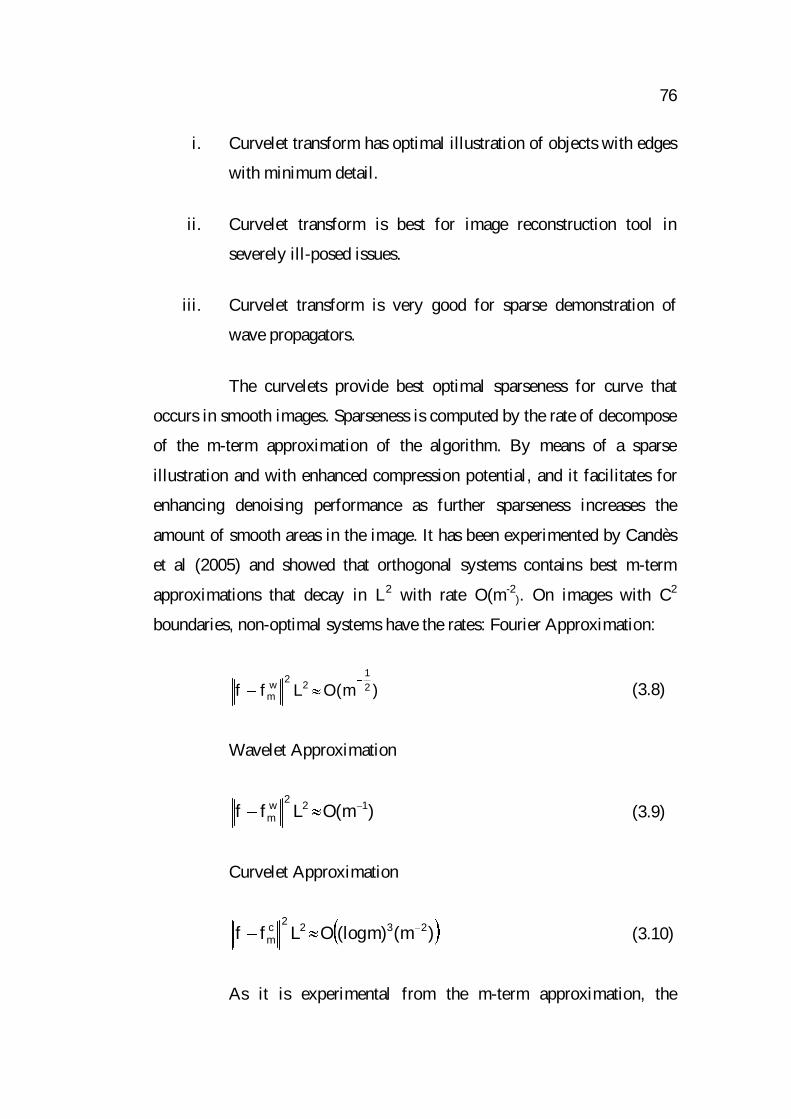
amount of smooth areas in the image. It has been experimented by Candès

et al (2005) and showed that orthogonal systems contains best m-term

approximations that decay in L2 with rate O(m-2). On images with C2

boundaries, non-optimal systems have the rates: Fourier Approximation:

)m(OLff 21

22wm (3.8)

Wavelet Approximation

)m(OLff 122wm (3.9)

Curvelet Approximation

)m()m(logOLff 2322cm (3.10)

As it is experimental from the m-term approximation, the

77

Curvelet Transform provides the closest m-term approximation to the

lesser bound. Thus, in images with a large numeral of C2 curves, curvelet

algorithm would be very effectual.

3.7.1 Continuous Curvelet Transform

Continuous curvelet transform has two major categories.

The primary continuous curvelet transform used a composite series of steps

comprising of the ridgelet assessment of an image with random transform

(Candes & Donoho 1999). The accuracy result of this algorithm was

tremendously slow. So, the algorithm was modified in 2003 (Candes &

Donoho 2003).

The utilization of the ridgelet transform was taken into

consideration, thus minimizing the quantity of redundancy in the transform

and ever-increasing the speed considerably. In 1994, Kashin & Temlyakov

considered this new approach of curvelets as tight frames. By means of

tight frames, a single curvelet has frequency support values in a parabolic-

wedge region. A sequence of curvelets k,l,j are tight frames which

presents definite value for A such that:

22

k,l,jk,l,j

22Lf:,fLfA (3.11)

where every curvelet in the space domain is defined as follows

)kxRD(2 j3j2

k,l,j (3.12)

With jD = Parabolic Scaling matrix, R = Rotation matrix,

k = translation parameter, = the “mother” curvelet by means of the

property of tight frames, the inverse of the curvelet transform is simply

78

established as Equation (3.13).

k,l,jk,l,jk,l,j

,ff (3.13)

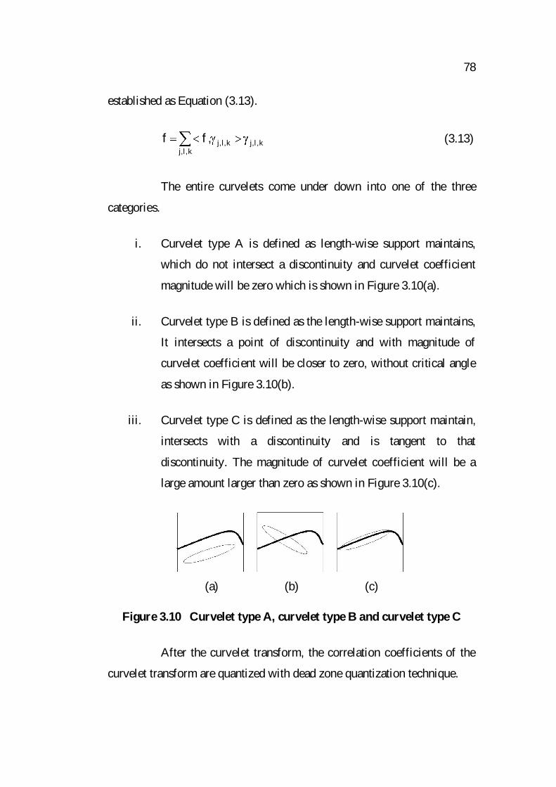
The entire curvelets come under down into one of the three

categories.

i. Curvelet type A is defined as length-wise support maintains,

which do not intersect a discontinuity and curvelet coefficient

magnitude will be zero which is shown in Figure 3.10(a).

ii. Curvelet type B is defined as the length-wise support maintains,

It intersects a point of discontinuity and with magnitude of

curvelet coefficient will be closer to zero, without critical angle

as shown in Figure 3.10(b).

iii. Curvelet type C is defined as the length-wise support maintain,

intersects with a discontinuity and is tangent to that

discontinuity. The magnitude of curvelet coefficient will be a

large amount larger than zero as shown in Figure 3.10(c).

(a) (b) (c)

Figure 3.10 Curvelet type A, curvelet type B and curvelet type C

After the curvelet transform, the correlation coefficients of the

curvelet transform are quantized with dead zone quantization technique.

79

3.7.2 Proposed Image Compression Algorithm

The proposed image compression technique is extremely

efficient by overcoming the issues of general wavelet transform based

coding compression algorithm which are applicable to the images with

linear curves. The steps involved in the proposed approach are:

i. Represent the image data as intensity values of pixels in the

spatial co-ordinates.

ii. Apply curvelet transform on the image matrix and get the

curvelet coefficients of the image.

iii. Quantize the available coefficients using dead zone quantization

algorithm.

iv. Use modified SPIHT coding on the bit stream.

Thus, the proposed image compression approach is based on

Curvelet Transformation with dead zone quantization and SPIHT, modified

SPIHT encoding and hybrid algorithm.

3.8 PERFORMANCE EVALUATION METRICS

The performance metrics taken for evaluation of these

approaches are:

3.8.1 Root Mean Square Error (RMSE) and Peak Signal to Noise

Ratio (PSNR)

Root Mean Square Error (RMSE) metric is extensively used for

it is easiness to compute, having obvious physical interpretation and

80

mathematically suitable. RMSE is computed by averaging the squared

intensity difference of reconstructed image x̂ , the original image, x.

The RMSE is calculated as Equation (3.14).

2)]j,i(x̂)j,i(x[MN2RMSE (3.14)

where )j,i(x is the original image, )j,i(x̂ approximated version

(which is actually the decompressed image) and M,N are the dimensions of

the images. MxN is the size of the image and assuming the grey scale

image of 8 bits per pixel (bpp), PSNR is defined as Equation (3.15).

MSE255log10PSNR

2

10 (3.15)

3.8.2 Compression Ratio

Compression ratio is used to enumerate the minimization in the

size of image representation, produced by an image compression

algorithm. The data compression ratio is equivalent to the physical

compression ratio used to evaluate physical compression of substances and

is defined as the ratio between the uncompressed image size and the

compressed image size.

3.8.3 Correlation

Correlation is used to measure the similarity of two images. If it

is close to 1, then two images are similar. Normalized cross-correlation can

be used to determine how to register or align the images by translating one

of them. It is calculated by Equation (3.16).

81

)Wj,i( 22

)Wj,i( 12

)Wj,i( 11

)jy,ix(I)j,i(I2

)jy,ix(I).j,i(I (3.16)

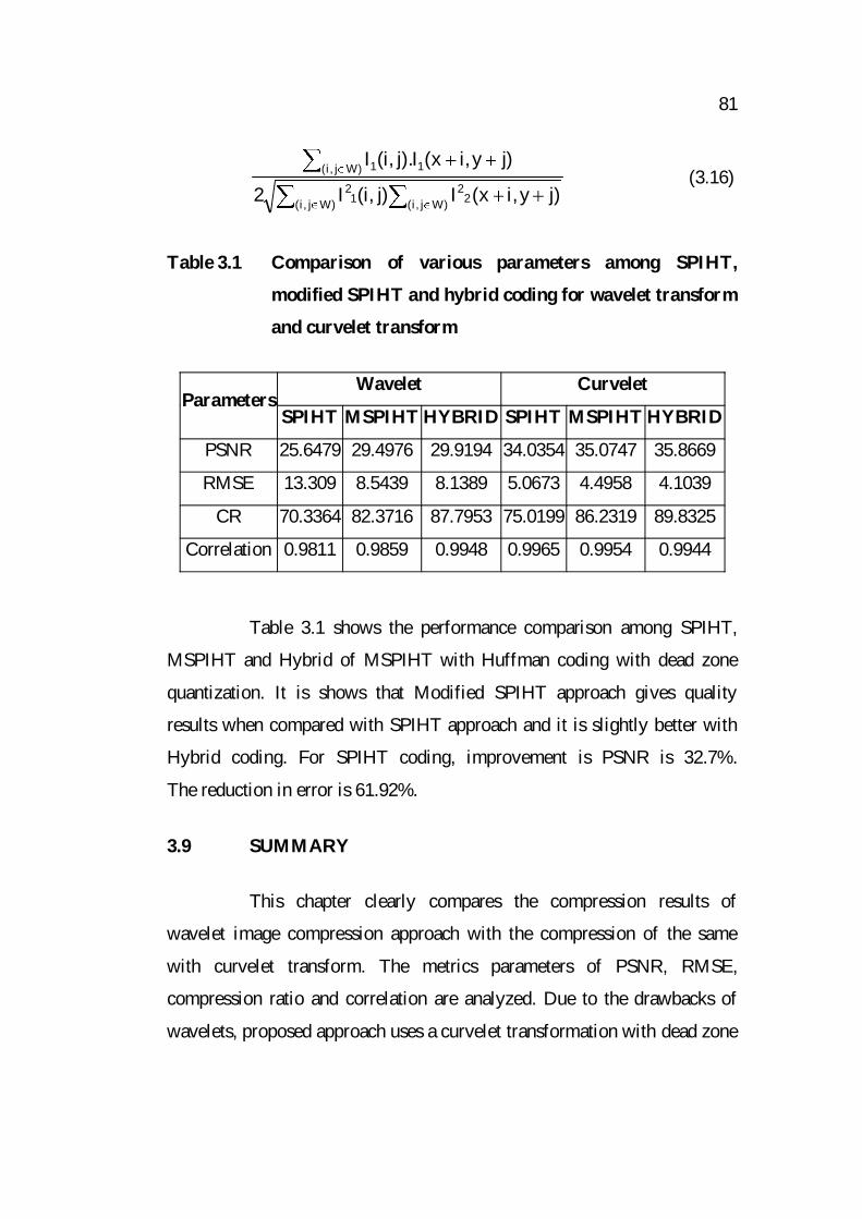
Table 3.1 Comparison of various parameters among SPIHT,

modified SPIHT and hybrid coding for wavelet transform

and curvelet transform

Parameters Wavelet Curvelet

SPIHT MSPIHT HYBRID SPIHT MSPIHT HYBRID

PSNR 25.6479 29.4976 29.9194 34.0354 35.0747 35.8669

RMSE 13.309 8.5439 8.1389 5.0673 4.4958 4.1039

CR 70.3364 82.3716 87.7953 75.0199 86.2319 89.8325

Correlation 0.9811 0.9859 0.9948 0.9965 0.9954 0.9944

Table 3.1 shows the performance comparison among SPIHT,

MSPIHT and Hybrid of MSPIHT with Huffman coding with dead zone

quantization. It is shows that Modified SPIHT approach gives quality

results when compared with SPIHT approach and it is slightly better with

Hybrid coding. For SPIHT coding, improvement is PSNR is 32.7%.

The reduction in error is 61.92%.

3.9 SUMMARY

This chapter clearly compares the compression results of

wavelet image compression approach with the compression of the same

with curvelet transform. The metrics parameters of PSNR, RMSE,

compression ratio and correlation are analyzed. Due to the drawbacks of

wavelets, proposed approach uses a curvelet transformation with dead zone

82

quantization approaches. Moreover, for the encoding purpose, SPIHT,

modified SPIHT and hybrid are used.