Chapter 3 Transport in one and two dimensions4 CHAPTER 3. TRANSPORT IN ONE AND TWO DIMENSIONS...
94
Chapter 3 Transport in one and two dimensions In this chapter, we consider transport in which there is a variation in the mass, momentum and temperature fields in one dimension. The analysis is considerably simplified in this case, since there is variation with respect to only one spatial co-ordinate, in addition to variation in time for unsteady diffusion and flow problems. However, the examples solved here illustrate the basic principles of the solution of more complex problems in multiple dimensions, which involve shell balances to derive differential equations for the concentration, velocity and temperature fields, and then an integration procedure for determining the variations in the concentration, velocity and temperature. 3.1 Transport between flat plates: The simplest configuration consists of two plates of infinite extent separated by length L, as shown in figure ??. There is a flux of mass, momentum or energy due to a difference in the concentration, velocity or temperature between the two plates. At steady state, there is a constant flux between the two plates in the direction perpendicular to the two plates, and the concentration, velocity or temperature varies linearly with the distance. One could also consider an unsteady situation, where the entire system is at a temperature T 0 , and the temperature of one plate is instanteneously changed to T 1 , as shown in figure ??. The equivalent situations in mass and 1
Transcript of Chapter 3 Transport in one and two dimensions4 CHAPTER 3. TRANSPORT IN ONE AND TWO DIMENSIONS...

Chapter 3
Transport in one and twodimensions
In this chapter, we consider transport in which there is a variation in themass, momentum and temperature fields in one dimension. The analysis isconsiderably simplified in this case, since there is variation with respect toonly one spatial co-ordinate, in addition to variation in time for unsteadydiffusion and flow problems. However, the examples solved here illustratethe basic principles of the solution of more complex problems in multipledimensions, which involve shell balances to derive differential equations forthe concentration, velocity and temperature fields, and then an integrationprocedure for determining the variations in the concentration, velocity andtemperature.
3.1 Transport between flat plates:
The simplest configuration consists of two plates of infinite extent separatedby length L, as shown in figure ??. There is a flux of mass, momentumor energy due to a difference in the concentration, velocity or temperaturebetween the two plates. At steady state, there is a constant flux betweenthe two plates in the direction perpendicular to the two plates, and theconcentration, velocity or temperature varies linearly with the distance.
One could also consider an unsteady situation, where the entire systemis at a temperature T0, and the temperature of one plate is instanteneouslychanged to T1, as shown in figure ??. The equivalent situations in mass and
1

2 CHAPTER 3. TRANSPORT IN ONE AND TWO DIMENSIONS
momentum transfer involves a system initially at constant concentration c0,in which the concentration of one plate is instanteneously set equal to c1. Inmomentum transfer, one could consider a system which is initially stationary,in which the velocity of one surface is set equal to U . The temperature,concentration or velocity is initially a step function, and then it evolves intime and finally approaches a steady linear temperature profile in the longtime limit.
In this chapter, we will also consider situations involving periodic oscil-lations in the temperature, concentration or velocity on one plate. In thecase of momentum transport, this involves one stationary plate and anotherplate oscillating at a fixed frequency. Similar situations can be consideredfor heat and mass transport. In all cases, we first derive equations for thevariation, both in position and time, of the concentration, temperature orvelocity in between the two plates. When expressed in terms of the scaledconcentration, temperature or velocity fields, these equations are identical inform. The solution procedures for these equations under steady and unsteadysituations are then discussed.
3.2 Cartesian co-ordinates:
3.2.1 Mass transfer
Consider two flat surfaces in the x − y plane, separated by a distance L,located at z = 0 and z = L. through which the solvent diffuses into thefluid, as shown in figure reffig311. The temperature is c0 at the top plate,and c1 at the bottom plate. An equation for the variation of concentrationwith z and with time can be derived from the mass conservation condition,
Consider a shell of thickness ∆z in the z coordinate as shown in figure 3.1,and of area ∆x∆y in the x−y plane. There is a transport of mass across thesurfaces of the shell due to diffusion, which results in a change in the concen-tration in the shell. We consider the variation in the concentration withinthis control volume over a time interval ∆t. Mass conservation requires that
(
Accumulation ofmass in the shell
)
=
(
Input ofmass into shell
)
−(
Output ofmass from shell
)
+
(
Production ofmass in shell
)
(3.1)
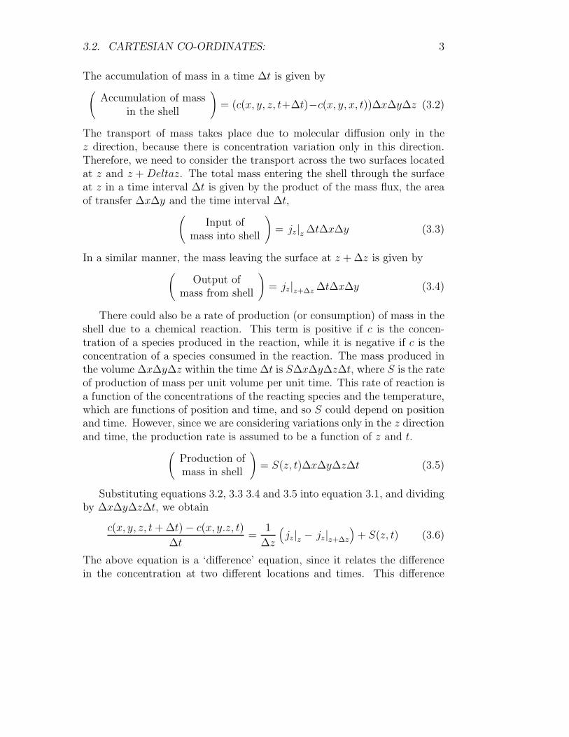
3.2. CARTESIAN CO-ORDINATES: 3
The accumulation of mass in a time ∆t is given by(
Accumulation of massin the shell
)
= (c(x, y, z, t+∆t)−c(x, y, x, t))∆x∆y∆z (3.2)
The transport of mass takes place due to molecular diffusion only in thez direction, because there is concentration variation only in this direction.Therefore, we need to consider the transport across the two surfaces locatedat z and z + Deltaz. The total mass entering the shell through the surfaceat z in a time interval ∆t is given by the product of the mass flux, the areaof transfer ∆x∆y and the time interval ∆t,
(
Input ofmass into shell
)
= jz|z ∆t∆x∆y (3.3)
In a similar manner, the mass leaving the surface at z + ∆z is given by(
Output ofmass from shell
)
= jz|z+∆z ∆t∆x∆y (3.4)
There could also be a rate of production (or consumption) of mass in theshell due to a chemical reaction. This term is positive if c is the concen-tration of a species produced in the reaction, while it is negative if c is theconcentration of a species consumed in the reaction. The mass produced inthe volume ∆x∆y∆z within the time ∆t is S∆x∆y∆z∆t, where S is the rateof production of mass per unit volume per unit time. This rate of reaction isa function of the concentrations of the reacting species and the temperature,which are functions of position and time, and so S could depend on positionand time. However, since we are considering variations only in the z directionand time, the production rate is assumed to be a function of z and t.
(
Production ofmass in shell
)
= S(z, t)∆x∆y∆z∆t (3.5)
Substituting equations 3.2, 3.3 3.4 and 3.5 into equation 3.1, and dividingby ∆x∆y∆z∆t, we obtain
c(x, y, z, t + ∆t) − c(x, y.z, t)
∆t=
1
∆z
(
jz|z − jz|z+∆z
)
+ S(z, t) (3.6)
The above equation is a ‘difference’ equation, since it relates the differencein the concentration at two different locations and times. This difference

4 CHAPTER 3. TRANSPORT IN ONE AND TWO DIMENSIONS
equation can be converted into a differential equation by taking the limit∆t → 0 and ∆z → 0.
∂c
∂t= −∂jz
∂z+ S (3.7)
Using the Fick’s law for diffusion,
jz = −D∂c
∂z(3.8)
the concentration diffusion equation 3.7 becomes,
∂c
∂t=
∂
∂z
(
D∂c
∂z
)
+ S (3.9)
The above equation is a ‘partial differential equation’, since it contains deriva-tives with respect to two independent variables, z and t. (This is in contrastto an ‘ordinary differential equation’, which contains derivatives with respectto only one independent variable).
If the diffusion coefficient is a constant (a good approximation in mostcases of practical interest), the differential equation 3.9 reduces to
∂c
∂t= D
∂2c
∂z2+ S (3.10)
3.2.2 Heat transfer:
The equivalent heat transfer problem involves two plates of temperature T0
at z = L, and temperature T1 at z = 0. A shell of of thickness ∆z in the zcoordinate, and of area ∆x∆y in the x − y plane, as shown in figure 3.1, isconsidered. The energy conservation condition is
(
Accumulation of energyin the shell
)
=
(
Input ofenergy into shell
)
−(
Output ofenergy from shell
)
+
(
Productionenergy in shell
(3.11)The accumulation of mass in a time ∆t is given by
(
Accumulation of energyin the shell
)
= (ρCp(T (x, y, z, t+∆t)−T (x, y, x, t)))∆x∆y∆z
(3.12)

3.2. CARTESIAN CO-ORDINATES: 5
The total heat entering the shell through the surface at z in a time interval∆t is given by the product of the heat flux, the area of transfer ∆x∆y andthe time interval ∆t,
(
Input ofheat into shell
)
= qz|z ∆x∆y∆t (3.13)
In a similar manner, the heat leaving the surface at z + ∆z is given by(
Output ofheat from shell
)
= qz|z+∆z ∆x∆y∆t (3.14)
The production (or consumption) of heat in the shell due to several rea-sons, such chemical reaction (exothermic or endothermic), heat of dissolution,latent heat due to phase transformations, or even due to viscous heating. Theheat produced in the volume ∆x∆y∆z within the time ∆t is Se∆x∆y∆z∆t,where Se is the rate of production of heat per unit volume per unit time. Asin the case of production of mass, we assume this is a function of z and time,
(
Production ofmass in shell
)
= Se(z, t)∆x∆y∆z∆t (3.15)
Substituting equations 3.12, 3.13 3.14 and 3.15 into equation 3.11, anddividing by ∆x∆y∆z∆t, we obtain
ρCp(T (x, y, z, t + ∆t) − T (x, y, z, t)
∆t=
qz|z − qz|z+∆z
∆z+ Se (3.16)
The above equation is a ‘difference’ equation, since it relates the differencein the concentration at two different locations and times. This differenceequation can be converted into a differential equation by taking the limit∆t → 0 and ∆z → 0.
ρCp∂T
∂t= −∂qz
∂z+ Se (3.17)
Using Fourier’s law for heat conduction,
qz = −k∂T
∂z(3.18)
the energy conservation equation can be written as,
ρCp∂T
∂t=
∂
∂z
(
k∂T
∂z
)
+ Se (3.19)

6 CHAPTER 3. TRANSPORT IN ONE AND TWO DIMENSIONS
If the thermal conductivity is independent of the z co-ordinate, the energyconservation equation can be written as,
∂T
∂t= α
∂
∂z
(
∂T
∂z
)
+Se
ρCp
(3.20)
where α = (k/ρCp) is the thermal diffusivity.
3.2.3 Momentum transport:
Though the final equation for the momentum transfer process is identicalto equations 3.10 and 3.20, the procedure is slightly different, and so weprovide a brief outline of the calculation. First, note that there are now twodirections in the problem. Since momemtum is a vector, there is a directionassociated with the momentum itself. In the present problem, this is the xdirection, because the velocity of the fluid is in the x direction. The secondis the direction of variation of the momentum, which is the z direction inthis problem, because the fluid velocity is varying only in the z direction.Since diffusion takes place along the direction where there is a variation ofmomentum, the diffusion in the present problem is also in the z direction.
The momentum balance equation (Newton’s third law), equivalent ofequation 3.1 and 3.11, is
Rate of change ofx momentumin the shell
=
(
Surface of forcesin x direction
)
+
(
Body forcesin x direction
)
(3.21)The total fluid mass in the differential volume is ρ∆x∆y∆z, where ρ is thefluid density and the volume of fluid is ∆x∆y∆z. We assume that the densityis a constant, so that the change in momentum (mass times velocity) is dueto the change in the velocity. The rate of change of momentum (change inmomentum per unit time) in the differential volume of thickness ∆z aboutz in a time interval ∆t is given by,
Rate of change ofx momentumin the shell
=(rho∆x∆y∆z)(ux(x, y, z, t + ∆t) − ux(x, y, z, t)
∆t
(3.22)The forces acting are of two types. The first is the ‘body force’, such
as the gravitational, centrifugal and other forces, which act throughout the

3.2. CARTESIAN CO-ORDINATES: 7
body. The second is the ‘surface force’ acting on the bounding surfaces,pressure and the shear stress. The body forces (centrifugal, gravitational,etc.) can be written as,
(
Body forcesin x direction
)
= fx∆x∆y∆z (3.23)
where fx is the force per unit volume in the x direction. The two importantbody forces we will encounter are the gravitational force fx = ρgx, whereρ is the mass density (mass per unit volume) and gx is the component ofthe acceleration due to gravity in the x direction, and the centrifugal force,fx = ρΩ2r, where Ω is the angular velocity and r is the distance from theaxis of rotation.
The surfaces forces acting on the two surfaces at z and z + ∆z are theproducts of the shear stress τxz and the surface area (∆x∆y). It is importantto keep account of the directions of the forces in this case, since the force isa vector. The shear stress τxz is defined as the force per unit area in the xdirection acting at a surface whose outward unit normal is in the positive zdirection. For the surface at z + ∆z, the outward unit normal is in the +zdirection, as shown in figure 3.1, and therefore the force per unit area at thissurface is + τxz|z+∆z. For the surface at z, the outward unit normal is in the−z direction, and therefore the force per unit area at this surface is − τxz|z.Therefore,
(
Surface of forcesin x direction
)
= ∆y∆z(τxz(z + ∆z, t) − τxz(z, t)) (3.24)
Therefore, the momentum balance equation is,
(∆x∆y∆z)ρ∆ux
∆t= ∆x∆y(τxz|z+∆z − τxz|z) + fx∆x∆y∆z (3.25)
Dividing throughout by A∆z, we obtain,
ρ∆ux
∆t=
τxz|z+∆z − τxz|z∆z
+ fx (3.26)
Taking the limit ∆t → 0 and ∆z → 0, we obtain the partial differentialequation,
ρ∂ux
∂t=
∂τxz
∂z+ fx (3.27)

8 CHAPTER 3. TRANSPORT IN ONE AND TWO DIMENSIONS
Note that f is a ‘force density’, which is the force acting per unit volume.The shear stress is given by the product of the viscosity and the gradient
of the velocity,
τxz = µ∂ux
∂z(3.28)
With this, the governing equation for the velocity field becomes,
ρ∂ux
∂t=
∂
∂z
(
µ∂ux
∂z
)
+ fx (3.29)
The differential equation derived above has the same form as the concentra-tion and energy diffusion equations 3.1 and 3.11, though it was derived froma force balance. This shows that the diffusion process is the same for mass,momentum and energy. However, it should be noted that momentum couldbe transmitted by pressure forces in addition to viscous forces, and there isno analogue of pressure in mass and energy transport.
The momentum conservation equation can be recast in terms of the mo-mentum diffusivity ν, if the viscosity and density are constants,
∂ux
∂t= ν
(
∂2ux
∂z2
)
+ (fx/ρ) (3.30)
where ν = (µ/rho) is the momentum diffusivity.
3.2.4 Steady and unsteady solutions:
We now solve the diffusion equation in a sequence of problems increasing incomplexity, starting from the steady solution, and then moving on to theunsteady solution in an infinite domain, the unsteady solution in a finitedomain, and finally a solution that is oscillatory in time. After this, weconsider the effect of sources of mass and energy, as well as body forcesexerted on the fluid.
At steady state, we solve the equations, for mass, momentum and energyconservation of the form,
∂2c
∂z2= 0;
∂2T
∂z2= 0;
∂2ux
∂z2= 0 (3.31)
with boundary conditions,
c = c1; T = T1; ux = U atz = 0 (3.32)
c = c0; T = T0; ux = U atz = H (3.33)

3.2. CARTESIAN CO-ORDINATES: 9
It is a good practice to first non-dimensionalise the co-ordinate z, as well asthe concentration, temperature and velocity. For this problem, it is appro-priate to use the scaling z∗ = (z/H), so that z∗ varies between 0 and 1 inthe domain between the plates. The scaled concentration, temperature andvelocity can be defined as,
c∗ =c − c0
c1 − c0(3.34)
T ∗ =T − T0
T1 − T0(3.35)
u∗x =
ux
U(3.36)
When scaled in this manner, the boundary conditions for the mass, momen-tum and energy transport problems are identical,
c∗ = T ∗ = u∗x = 1 at z∗ = 0 (3.37)
c∗ = T ∗ = u∗x = 0 at z∗ = 1 (3.38)
It is quite easy to obtain the linear solutions for the concentration, temper-ature and velocity equations, 3.31, which satisfy the boundary conditions3.38,
c∗ = T ∗ = u∗x = 1 − z∗ (3.39)
As expected, the concentration, temperature and velocity profiles are linearbecause the fluxes are constant.
3.2.5 Unsteady transport into an infinite fluid:
Let us now consider the unsteady state transport of mass/momentum/heatin a fluid between two flat plates, as shown in figure ??, with no sources.In the mass transfer problem, the fluid and both plates are initially at aconcentration c0. At time t = 0, the temperature of the lower plate isinstanteneously set equal to c1 > c0. There is a heat flux from the bottomplate, and the temperature increases upwards. In the final steady state,the linear concentration profile equation 3.39 is obtained. Here, we shall beconcerned with the very initial stages, when the ‘penetration depth’ from thebottom surface is small compared to the distance between the two plates, L.In this case, the we can consider the region near the bottom plate alone,and consider the fluid to be of infinite extent in the z direction. Instead of

10 CHAPTER 3. TRANSPORT IN ONE AND TWO DIMENSIONS
the boundary condition equation 3.38, we can use the boundary conditionsc = c1 at z = 0 and c = c0 as z → ∞. The initial condition is c = c0 for allz > 0 at t = 0. The mass diffusion equation is 3.31, and the boundary andinitial conditions are,
c = 0 as z → ∞ at all t (3.40)
c = c0 at z = 0 at all t > 0 (3.41)
c = 0 at t = 0 for all z > 0 (3.42)
The scaled concentration field c∗ is defined in equation 3.34, and theconditions for c∗ are
c∗ = 0 as z → ∞ at all t (3.43)
c∗ = 1 at z = 0 at all t > 0 (3.44)
c∗ = 0 at t = 0 for all z > 0 (3.45)
The diffusion equation for the concentration field is,
∂c∗
∂t= D
∂2c∗
∂z2(3.46)
In the equivalent heat and momentum transfer problems, we substituteT ∗ and u∗
x instead of c∗, and the thermal diffusivity α and kinematic viscosityν instead of the mass diffusivity D.
In order to solve the concentration equation 3.46 with the boundary andinitial conditions 3.45, it is first important to realise that there no intrinsiclength scale in the problem, because the boundary conditions are applied atz∗ = 0 and z∗ → ∞. Since the concentration c∗ is dimensionless, there areonly three dimensional variables z, t and D in the problem. These contain twodimensions, L and T , and it is possible to construct only one dimensionlessnumber, ξ = (z/
√Dt). Therefore, just from dimensional analysis, it can be
concluded that the concentration field does not vary independently with zand t, but depends only on the combination ξ = (z/
√Dt). If this inference
is correct, it should be possible to express the conservation equation 3.46 interms of the variable ξ alone. When z and t are expressed in terms of ξ, theconcentration equation becomes
−(
z
2D1/2t3/2
)
∂c∗
∂ξ=
D
Dt
∂2c∗
∂ξ2(3.47)

3.2. CARTESIAN CO-ORDINATES: 11
c*=1T*=1u*=1x
x
zz
∆z+ z
z=0
c*=0T*=0u*=0x
z−−>Infinity
Figure 3.1: Configuration for similarity solution for unidirectional transport.

12 CHAPTER 3. TRANSPORT IN ONE AND TWO DIMENSIONS
After multiplying throughout by t, the equation for the concentration fieldreduces to
ξ
2
∂c∗
∂ξ+
∂2c∗
∂ξ2= 0 (3.48)
Equation 3.48 validates the earlier inference, based on dimensional analysis,that the non-dimensionalised concentration field is only a function of ξ, andcontains z, t or D only in the combination (z/
√Dt).
It is also necessary to transform the boundary and initial conditions, 3.43,3.44 and 3.45 into conditions for the ξ coordinate. The transformed boundaryconditions are
c∗ = 0 as z → ∞ at all t → as ξ → ∞ (3.49)
c∗ = 1 at z = 0 at all t > 0 → at ξ = 0 (3.50)
c∗ = 0 at t = 0 for all z > 0 → as ξ → ∞ (3.51)
Note that the original conservation equation, 3.46, is a second order differ-ential equation in z and a first order differential equation in t, and so thisrequires two boundary conditions in the z coordinate and one initial condi-tion. The conservation equation expressed in terms of ξ is a second orderdifferential equation, which requires just two boundary conditions for ξ. Fromequation 3.50 and 3.51, it can be seen that one of the boundary conditionsfor z → ∞ (equation 3.43) and the initial condition t = 0 (equation 3.45)turn out to be identical conditions for ξ → ∞.
Equation 3.48 is a second order ordinary differential equation for c∗(ξ),which can be easily solved to obtain
c∗(ξ) = C1 + C2
∫ ∞
ξdξ′ exp
(
−ξ′2
4
)
(3.52)
The constants C1 and C2 are determined from the conditions c∗ = 1 at ξ = 0,and c∗ = 0 for ξ → ∞, to obtain
c∗(z/√
Dt) =
(
1 − 1√π
∫ (z/√
Dt)
0dξ′ exp
(
−ξ′2
4
))
(3.53)
The solution 3.53 for c∗(z/√
Dt) is shown as a function of (z/√
Dt) infigure 3.2. From this solution, we see that c∗ decreases to about 0.48 at(z/
√Dt) = 1.0, and to about 0.16 at (z/
√Dt) = 2.0,and further to about
0.034 at (z/√
Dt) = 3.0. For (z/√
Dt) > 3.0, the scaled concentration field is

3.2. CARTESIAN CO-ORDINATES: 13
0 1 2 3 4 5(z/√Dt)
0
0.1
0.2
0.3
0.4
0.5
0.6
0.7
0.8
0.9
1
c∗ (z/√
Dt)
Figure 3.2: The solution equation 3.53 for c∗(z/√
Dt) as a function of(z/
√Dt).
close to zero. Therefore, the length scale for the variation of the concentration(penetration depth) is
√Dt. This length scale is a function of time, and it
increases proportional to t1/2.
As discussed at the beginning of this section, the solution equation 3.53is valid only when the penetration depth is small compared to the distancebetween plates, or
√Dt ≪ H , or t ≪ (H2/D). When the penetration depth
becomes comparable to H , a similarity solution cannot be used, because thelength scale H is also relevant, and the scaled z co-ordinate can be defined asz∗ = (z/H). The similarity reduction here was possible because the boundaryconditions 3.49 and 3.50 were applied at z = 0 and z → ∞ respectively. Sincethere is no other length scale, there are three dimensional quantities, z, t andD, and from these it was possible to form only one dimensionless group onthe basis of dimensional analysis. However, the similarity solution method ismore general, and does not rely on dimensional analysis alone, as shown inthe next problem. This method forms the basis of boundary layer theories

14 CHAPTER 3. TRANSPORT IN ONE AND TWO DIMENSIONS
to be discussed later.
3.2.6 Steady diffusion into a falling film
This problem is a simplification of the actual diffusion in a falling film, whichinvolves a combination of convection and diffusion. We discuss this now,even though it is not an unsteady diffusion problem, because the solutionis a similarity solution similar to that for unsteady diffusion into an infinitefluid.
A thin film of fluid flows down a vertical surface with a constant velocityU in the x direction. At the gas-liquid interface, the liquid is in contact with agas which is soluble in the liquid. The concentration of gas in the liquid at theentrance is c0, while the concentration of gas at the liquid-gas interface is c1.The difference in concentration between the initial concentration in the liquidand the concentration at the interface acts as a driving force for diffusion. Thez coordinate is perpendicular to the gas-liquid interface, which is located atz = 0. As the liquid flows down, the gas is dissolved in the liquid and carriedby the fluid in the streamwise x direction, as shown in figure ??. Therefore,there is a variation in concentration with the z co-ordinate. However, thesystem is at steady state, and does not vary in time.
The mass conservation equation can be obtained by carrying out a shellbalance over a differential volume, as shown in figure ??. In this case, thereis transport due to fluid convection in the streamwise (x) direction, anddiffusion due to a concentration gradient in the z direction. There is diffusionin the x direction as well, because the concentration is not a constant inthat direction. However, under certain conditions (which we will discuss atthe end), the diffusion in this direction is much smaller the the convectivetransport due to the mean fluid flow.
The terms in the mass balance equation, 3.1, are as follows. Since thesystem is at steady state, there is no change in the concentration with time,and the term on the left side of equation 3.1 is zero. There is mass enteringthe differential volume at the right surfaces at z, and mass leaving at the leftsurface at z +∆z, and z +∆z due to diffusion. These are given by equations3.3 and 3.4. In addition, there is also mass entering the top surface at x, andleaving the bottom surface at x + ∆x due to convection,
(
Mass enteringsurface at x
)
= Uc|x ∆y∆z (3.54)

3.2. CARTESIAN CO-ORDINATES: 15
(
Mass leavingsurface at x + ∆x
)
= Uc|x+∆x ∆y∆z (3.55)
Therefore, the mass balance equation is,
jz|z ∆x∆y − jz|z+∆z ∆x∆y + Uc|x ∆y∆z − Uc|x+∆x ∆y∆z = 0 (3.56)
If the above equation is divided by ∆x∆y∆z, we obtain,
jz|z − jz|z+∆z
∆z+
Uc|x − Uc|x+∆x
∆x= 0 (3.57)
Taking the limit ∆x → 0 and ∆z → 0, we obtain,
∂(Uc)
∂x= −∂jz
∂z(3.58)
The Fick’s law for the mass flux, jz = −D(∂c/∂z), is substituted into equa-tion 3.57, to obtain,
U∂c
∂x= D
∂2c
∂z2(3.59)
Here, the term on the left has been simplified because the velocity U is aconstant. Using equation 3.34 for the scaled concentration field, the diffusionequation becomes,
U∂c∗
∂x= D
∂2c∗
∂z2(3.60)
Two boundary conditions are required in the z direction, since equation3.60 is a second order differential equation in the z, while one ‘initial’ condi-tion is required in the x direction equation 3.60 is first order in x. In the zdirection, the concentration at the liquid gas interface at z = 0 is c1, whilethe concentration far from the surface in the limit z → ∞ is c0. Therefore,the boundary condition for the scaled concentration field is,
c∗ = 1 atz = 0 (3.61)
c∗ = 0 forz → ∞ (3.62)
In addition, the concentration at x ≤ 0 is c0, for all z, because the liquid hasnot yet come into contact with the gas. Therefore, the ‘initial’ condition atx = 0 is,
c∗ = 0 atx = 0 for z ¿ 0 (3.63)
16 CHAPTER 3. TRANSPORT IN ONE AND TWO DIMENSIONS
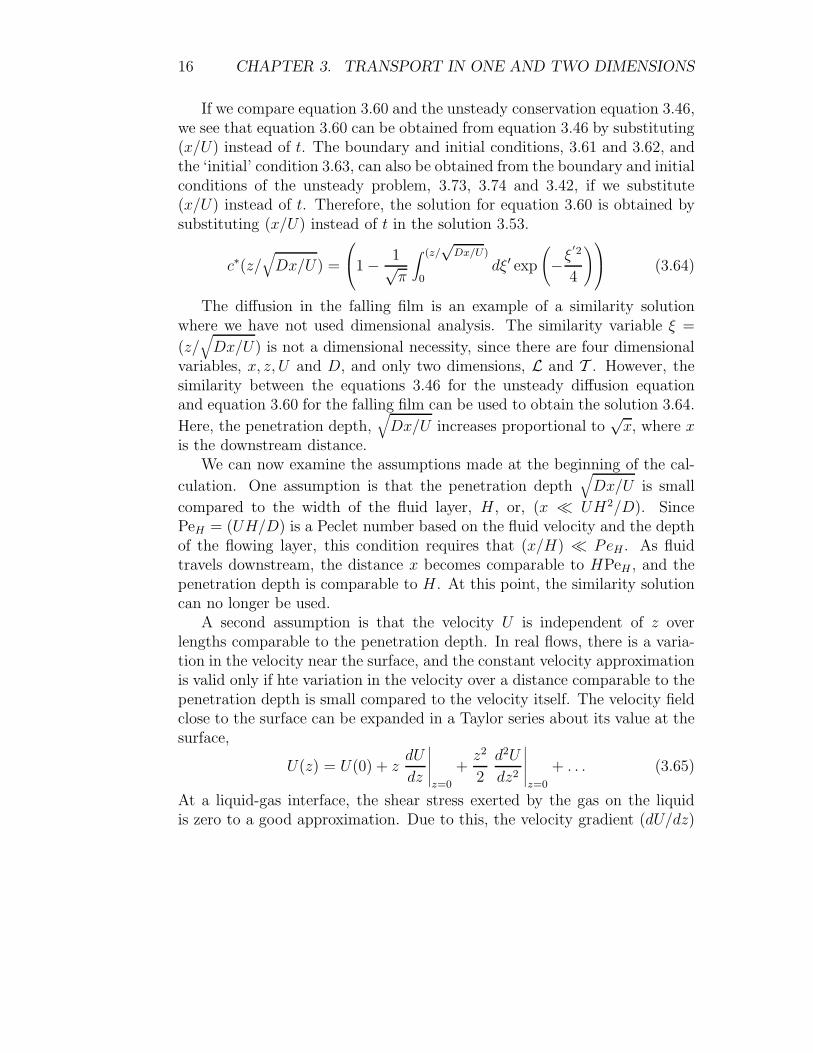
If we compare equation 3.60 and the unsteady conservation equation 3.46,we see that equation 3.60 can be obtained from equation 3.46 by substituting(x/U) instead of t. The boundary and initial conditions, 3.61 and 3.62, andthe ‘initial’ condition 3.63, can also be obtained from the boundary and initialconditions of the unsteady problem, 3.73, 3.74 and 3.42, if we substitute(x/U) instead of t. Therefore, the solution for equation 3.60 is obtained bysubstituting (x/U) instead of t in the solution 3.53.
c∗(z/√
Dx/U) =
1 − 1√π
∫ (z/√
Dx/U)
0dξ′ exp
(
−ξ′2
4
)
(3.64)
The diffusion in the falling film is an example of a similarity solutionwhere we have not used dimensional analysis. The similarity variable ξ =
(z/√
Dx/U) is not a dimensional necessity, since there are four dimensionalvariables, x, z, U and D, and only two dimensions, L and T . However, thesimilarity between the equations 3.46 for the unsteady diffusion equationand equation 3.60 for the falling film can be used to obtain the solution 3.64.
Here, the penetration depth,√
Dx/U increases proportional to√
x, where xis the downstream distance.
We can now examine the assumptions made at the beginning of the cal-
culation. One assumption is that the penetration depth√
Dx/U is small
compared to the width of the fluid layer, H , or, (x ≪ UH2/D). SincePeH = (UH/D) is a Peclet number based on the fluid velocity and the depthof the flowing layer, this condition requires that (x/H) ≪ PeH . As fluidtravels downstream, the distance x becomes comparable to HPeH , and thepenetration depth is comparable to H . At this point, the similarity solutioncan no longer be used.
A second assumption is that the velocity U is independent of z overlengths comparable to the penetration depth. In real flows, there is a varia-tion in the velocity near the surface, and the constant velocity approximationis valid only if hte variation in the velocity over a distance comparable to thepenetration depth is small compared to the velocity itself. The velocity fieldclose to the surface can be expanded in a Taylor series about its value at thesurface,
U(z) = U(0) + zdU
dz
∣
∣
∣
∣
∣
z=0
+z2
2
d2U
dz2
∣
∣
∣
∣
∣
z=0
+ . . . (3.65)
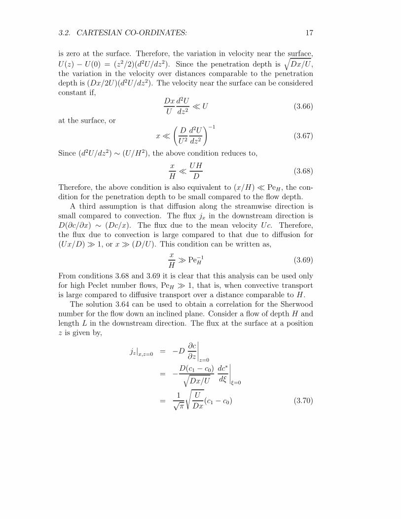
At a liquid-gas interface, the shear stress exerted by the gas on the liquidis zero to a good approximation. Due to this, the velocity gradient (dU/dz)
3.2. CARTESIAN CO-ORDINATES: 17
is zero at the surface. Therefore, the variation in velocity near the surface,
U(z) − U(0) = (z2/2)(d2U/dz2). Since the penetration depth is√
Dx/U ,the variation in the velocity over distances comparable to the penetrationdepth is (Dx/2U)(d2U/dz2). The velocity near the surface can be consideredconstant if,
Dx
U
d2U
dz2≪ U (3.66)
at the surface, or
x ≪(
D
U2
d2U
dz2
)−1
(3.67)
Since (d2U/dz2) ∼ (U/H2), the above condition reduces to,
x
H≪ UH
D(3.68)
Therefore, the above condition is also equivalent to (x/H) ≪ PeH , the con-dition for the penetration depth to be small compared to the flow depth.
A third assumption is that diffusion along the streamwise direction issmall compared to convection. The flux jx in the downstream direction isD(∂c/∂x) ∼ (Dc/x). The flux due to the mean velocity Uc. Therefore,the flux due to convection is large compared to that due to diffusion for(Ux/D) ≫ 1, or x ≫ (D/U). This condition can be written as,
x
H≫ Pe−1
H (3.69)
From conditions 3.68 and 3.69 it is clear that this analysis can be used onlyfor high Peclet number flows, PeH ≫ 1, that is, when convective transportis large compared to diffusive transport over a distance comparable to H .
The solution 3.64 can be used to obtain a correlation for the Sherwoodnumber for the flow down an inclined plane. Consider a flow of depth H andlength L in the downstream direction. The flux at the surface at a positionz is given by,
jz|x,z=0 = −D∂c
∂z
∣
∣
∣
∣
∣
z=0
= −D(c1 − c0)√
Dx/U
dc∗
dξ
∣
∣
∣
∣
∣
ξ=0
=1√π
√
U
Dx(c1 − c0) (3.70)
18 CHAPTER 3. TRANSPORT IN ONE AND TWO DIMENSIONS
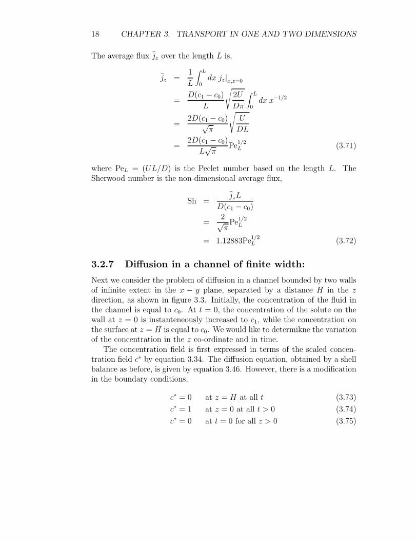
The average flux jz over the length L is,
jz =1
L
∫ L
0dx jz|x,z=0
=D(c1 − c0)
L
√
2U
Dπ
∫ L
0dx x−1/2
=2D(c1 − c0)√
π
√
U
DL
=2D(c1 − c0)
L√
πPe
1/2L (3.71)
where PeL = (UL/D) is the Peclet number based on the length L. TheSherwood number is the non-dimensional average flux,
Sh =jzL
D(c1 − c0)
=2√π
Pe1/2L
= 1.12883Pe1/2L (3.72)
3.2.7 Diffusion in a channel of finite width:
Next we consider the problem of diffusion in a channel bounded by two wallsof infinite extent in the x − y plane, separated by a distance H in the zdirection, as shown in figure 3.3. Initially, the concentration of the fluid inthe channel is equal to c0. At t = 0, the concentration of the solute on thewall at z = 0 is instanteneously increased to c1, while the concentration onthe surface at z = H is equal to c0. We would like to determikne the variationof the concentration in the z co-ordinate and in time.
The concentration field is first expressed in terms of the scaled concen-tration field c∗ by equation 3.34. The diffusion equation, obtained by a shellbalance as before, is given by equation 3.46. However, there is a modificationin the boundary conditions,
c∗ = 0 at z = H at all t (3.73)
c∗ = 1 at z = 0 at all t > 0 (3.74)
c∗ = 0 at t = 0 for all z > 0 (3.75)

3.2. CARTESIAN CO-ORDINATES: 19
c*=1T*=1u*=1x
x
zz
∆z+ z
z=0
c*=0T*=0u*=0x
z=L
Figure 3.3: Configuration for similarity solution for unidirectional transport.
In this case, it is not possible to reduce the problem using a similarity trans-form, because there is an additional length scale L in the problem, and sothe z coordinate can be scaled by H . A scaled z coordinate is defined asz∗ = (z/L), and the diffusion equation in terms of this coordinate is
∂c∗
∂t=
D
L2
∂2c∗
∂z∗2(3.76)
The above equation suggests that it is appropriate to define a scaled timecoordinate t∗ = (Dt/L2), and the conservation equation in terms of thisscaled time coordinate is
∂c∗
∂t∗=
∂2c∗
∂z∗2(3.77)
The boundary conditions, in terms of the scaled coordinates z∗ and t∗, are
c∗ = 0 at z∗ = 1 at all t∗ (3.78)
c∗ = 1 at z∗ = 0 at all t∗ > 0 (3.79)
c∗ = 0 at t∗ = 0 for all z∗ > 0 (3.80)
We briefly note that similar problems can be framed for heat and momen-tum transfer. In the heat transfer problem, the two plates and the fluid are

20 CHAPTER 3. TRANSPORT IN ONE AND TWO DIMENSIONS
initially at temperature T0. At t = 0, the temperature of the bottom plate isinstanteneously increased to T1. In the momentum transfer problem, the fluidand the two plates are initially at rest. At t = 0, a constant velocity ux = Uis imparted to the bottom plate. In both cases, non-dimensional concentra-tion, temperature and velocity fields can be defined according to equations3.34, 3.35 and 3.36. The conservation equations for the scaled temperatureand velocity fields are identical to equation 3.77, except that t∗ = (tα/H2)for the heat transfer problem, and t∗ = (tν/H2) for the momentum transferproblem. The boundary and initial conditions for T ∗ and u∗
x are also iden-tical to equations 3.78, 3.79 and 3.80. Therefore, the solutions for the T ∗
and u∗x are identical to those obtained here for c∗, except for the definition of
the dimensionless time t∗ which contains the thermal diffusivity in the heattransfer problem, and the momentum diffusivity in the momentum transferproblem.
The solution method involves separating the concentration field into asteady and transient part. In the long time limit, t∗ → ∞, the concentrationfield will attain a steady state value c∗s which is independent of time. Thissteady state concentration field is obtained by solving 3.77 with the timederivative set equal to zero, and the solution for the steady concentrationfield is a linear concentration profile in equation 3.39,
c∗s = (1 − z∗) (3.81)
The concentration can be separated into a steady and a transient part,
c∗ = c∗s + c∗t , (3.82)
where c∗t is the difference between the actual concentration and the concen-tration at steady state. The reason for this decomposition will become cleara little later.
The conservation equation for the unsteady concentration field is iden-tical to that for the original concentration field, because (∂c∗s/∂t∗) = 0 and(∂2c∗s/∂z∗2) = 0,
∂c∗t∂t∗
=∂2c∗t∂z∗2
(3.83)
However, the boundary condition for c∗t is different from that for the c∗, andis obtained by subtracting c∗s from c∗ at the boundaries,
c∗t = 0 at z∗ = 1 at all t∗ (3.84)
3.2. CARTESIAN CO-ORDINATES: 21
c∗t = 0 at z∗ = 0 at all t∗ > 0 (3.85)
c∗t = −c∗s at t∗ = 0 for all z∗ > 0 (3.86)
Equation 3.83 can be solved by the method of ‘separation of variables’,where the unsteady concentration field is expressed as two functions, one ofwhich is only a function of t∗, while the other is only a function of z∗.
c∗t = Θ(t∗)Z(z∗) (3.87)
This is inserted into the conservation equation 3.83, and the equation isdivided by the production ΘZ, to obtain
1
Θ
dΘ
dt∗=
1
Z
d2Z
dz∗2(3.88)
In equation 3.88, the left side is only a function of t∗, while the right sideis only a function of z∗. From this, it can be inferred, as follows, that thesetwo functions have to be constants independent of z∗ and t∗. To infer this,assume that these two functions are not constants, and that the left sidevaries as t∗ is varied, and the right side varies as z∗ is varied. In this case,if we keep z∗ a constant and vary t∗, then the left side of 3.88 varies, whilethe right side remains a constant, and so the equality is destroyed. The onlyway for the equality to hold, if the left side is only a function of t∗ and theright side is only a function of z∗, is if the two sides are constants.
The solution for Z is first obtained by solving
1
Z
d2Z
dz∗2= −α2 (3.89)
where α is a positive constant. The reason for choosing the right side of3.89 to be negative will become apparent a little later. The solution for thisequation is
Z = C1 sin (αz∗) + C2 cos (αz∗) (3.90)
where C1 and C2 are constants to be determined from the boundary con-ditions. The boundary condition c∗u = 0 (Z = 0) at z∗ = 0 is satisfied forC2 = 0. The boundary condition cau = 0 at z∗ = 1 is satisfied if α = (nπ),where n is an integer. Therefore, the solution for Z which satisfied theboundary conditions in the z∗ coordinate is
Z = C1 sin (nπz∗) (3.91)

22 CHAPTER 3. TRANSPORT IN ONE AND TWO DIMENSIONS
where n is an integer.The solution for Θ can now be obtained from the equation
1
Θ
dΘ
dt∗= −α2 = −n2π2 (3.92)
This equation is solved to obtain
Θ = C3 exp (−n2π2t∗) (3.93)
The final solution for c∗t = Θ(t∗)Z(z∗) is
c∗t = C exp (−n2π2t∗) sin (nπz∗) (3.94)
The solution 3.94 contains the integer n which is as yet unspecified, and thesolution 3.94 satisfies the equation 3.83 for any value of n. The most generalsolution is one which contains a linear combination of the solution 3.94 fordifferent values of n,
c∗t =∞∑
n=1
Cn exp (−n2π2t∗) sin (nπz∗) (3.95)
The values of the coefficients Cn have to be determined from the initialcondition that has not been used so far,
c∗t = −(1 − z∗) for t∗ = 0∞∑
n=1
Cn sin (nπz∗) = −(1 − za) (3.96)
The coefficients can be determined because the functions sin (nπz∗) satisfy‘orthogonality conditions’,
∫ 1
0dz∗ sin (nπz∗) sin (mπz∗) = 0 for n 6= m
= (1/2) for n = m (3.97)
To use this condition, the left and right sides of 3.98 are multiplied bysin (mπz∗), and integrated over the interval 0 ≤ z∗ ≤ 1, to obtain
Cm = −2∫ 1
0dz∗ sin (mπz∗)(1 − z∗)
= − 2
mπfor odd n (3.98)

3.2. CARTESIAN CO-ORDINATES: 23
Therefore, the final solution for the concentration field, which includes thesteady part (c∗s = (1 − z∗)) and the transient part is,
c∗z = (1 − z∗) −∞∑
n=1
2
nπsin (nπz∗) exp (−n2π2t∗) (3.99)
It is now time to examine the reason for choosing the constant on the rightside of 3.89 as a negative number. If we had chosen the right side of 3.89 tobe positive, the solution for Z consists of an exponentially growing and anexponentially decaying function. In this case, it can easily be verified thatthe boundary condtions c∗t = 0 at z∗ = 0 and at z∗ = 1 can be satisfied onlyif C1 = 0 and C2 = 0. In addition, the solution for Θ in equation 3.93 wouldhave been a function that is exponentially increasing in time, and therefore,there is no steady solution in this case. Since we have chosen the constantto be negative, the unsteady solution c∗t decays exponentially in time, andgoes to zero in the long time limit. Also, the solutions for Z(z∗) are sinefunctions, which can be chosen to satisfy the conditions c∗t = 0 at z∗ = 0 andz∗ = 1.
Further, the separating the concentration field into a steady and a tran-sient part is also now clear. The transient part of the concentration field hashomogeneous boundary conditions (c∗t = 0) at both the spatial boundaries,z∗ = 0 and z∗ = 1. However, the initial condition (c∗t = −c∗s at t∗ = 0)is inhomogeneous. Therefore, there is no forcing for the transient part ofthe concentration field at the boundaries, but there is forcing at the initialtime t∗ = 0. The concentration field generated by the forcing at t∗ = 0 thendecays exponentially with time.
The homogeneous spatial boundary conditions c∗t = 0 at z∗ = 0 andz∗ = 1 is also essential for another reason. In equation 3.91, we were able toobtain discrete values for the constant α = nπ only because the solution wasa sine function with Z = 0 at z∗ = 0 and 1. This enabled us to get a discrete‘spectrum’ of solutions with discrete eignevalues (nπ) and a correspondingset of basis functions sin (nπz∗). The solution Z(z∗) was then written as alinear combination of these eigen functions.
The ‘orthogonality’ conditions 3.97 for determining the constants Cn inequation 3.98 can be physically interpreted as follows. We define the basisfunctions Sn = sin (nπz∗), and we define the inner product
〈Sn, Sm〉 =∫ 1
0dz∗ sin (nπz∗) sin (mπz∗) (3.100)

24 CHAPTER 3. TRANSPORT IN ONE AND TWO DIMENSIONS
This inner product is non-zero only when n = m, and is zero when n 6= m,
〈Sn, Sm〉 =δnm
2(3.101)
where ‘Kronecker delta’ δnm = 1 for n = m, and δnm = 0 for n 6= m. Thebasis functions Sn are analogous to the basis vectors in a three-dimensionalco-ordinate system, while the ‘inner product’ is analogous to the dot productof unit vectors. The dot product of basis vector with another basis vectoris zero, sinc they are perpendicular to each other. In a similar manner, theinner product of two different basis functions is zero, and they are orthogonalto each other. However, there is an infinite number of basis functions for thesolution 3.99 for c∗, in contrast to the three unit vectors in three dimensionalspace.
The concept of inner products can be used to express the orthogonalityconditions in a compact manner. In this, the solution 3.95 for c∗t can bewritten as,
c∗t (z∗, t∗) =
∞∑
n=0
CnSn exp (−n2π2t∗) (3.102)
At t∗ = 0, the initial condition is c∗t = −c∗s = −(1 − z∗). Therefore,
∞∑
n=0
CnSn = −(1 − z∗) (3.103)
We take the inner product of both right and left sides with the basis functionSm.
∞∑
n=0
Cn〈Sm, Sn〉 = −〈(1 − z∗), Sm〉 (3.104)
Due to the orthogonality relation 3.101, the above equation reduces to
∞∑
n=0
Cn(δmn/2) = (Cm/2) = −〈(1 − z∗), Sm〉 (3.105)
In the summation on the left, δmn is zero only when m = n, and so theentire summation reduces to (Cm/2). Thus, the orthogonality condition 3.105enables us to determine all the constants in the expansion 3.95, and constructthe final solution.
Physically, we are expanding the solution Z(z∗) in a set of basis functionsSn = sin (nπz∗), which consists of a set of sine functions as shown in figure

3.2. CARTESIAN CO-ORDINATES: 25
??. This is a complete basis set, and any function can be expressed as a linearcombination of these basis functions. The basis functions are also orthogonal,because the inner product of two different basis functions (equation 3.100)is zero. This orthogonality condition is used to obtain the coefficients inthe expansion for Z(z∗). This procedure, of expanding the solutions in acomplete and orthogonal basis set, and using the orthogonality relations todetermine the terms in the expansions, will be used whenever the separationof variables procedure is carried out.
The solution 3.99 for c∗ is a summation over an infinite set of basisfunctions Sn, and so an exact solution requires the evaluation of an infi-nite number of terms. However, the nth term in the series is proportionalto exp (−n2π2t∗). Therefore, at a fixed time t∗, it is possible to get a goodnumerical approximation c∗≈ by truncating the series at a finite value of n.The value of n required to obtain the desired accuracy can be estimated asfollows. The error Ec∗(p), which is the difference between the exact solu-tion c∗ and the approximate solution c∗≈ obtained by truncating the series atn = p − 1, and neglecting terms for n ≥ p, is,
Ec∗(p) = c∗ − c∗≈
=∞∑
n=p
2
nπsin (nπz) exp (−n2π2t∗) (3.106)
Since the modulus of sin (nπz∗), the upper bound on the incurred in theapproximation is,
E∗c
max(p) =∞∑
n=p
2
nπexp (−n2π2t∗) (3.107)
For large values of n, the above summation can be approximated by anintegral,
E∗c
max(p) =∫ ∞
pdn(
2
nπexp (−n2π2t∗)
)
≤∫ ∞
(p/π√
t∗)dn′
(
2
n′πexp (−n
′2))
(3.108)
The function E∗c
max(p) is shown as a function of (p/π√
t∗) in figure 3.4.This upper bound on the error decreases quite rapidly with an increase in(p/π
√t∗). It is less than 0.05 for p ≥ 1.1π
√t∗, and it is less than 0.01

26 CHAPTER 3. TRANSPORT IN ONE AND TWO DIMENSIONS
0 0.2 0.4 0.6 0.8 1 1.2 1.4 1.6 1.8 2(p/(π √t∗ ))
0
0.5
1
1.5
2
2.5
Ec∗m
ax(p
)
Figure 3.4: The upper bound on the error, E∗c
max(p) (equation 3.108), as afunction of (p/π
√t∗).

3.2. CARTESIAN CO-ORDINATES: 27
for p ≥ 1.52π√
t∗. Thus, good numerical solutions can be obtained with arelatively small number of terms in the series expansion equation 3.99.
The numerical solutions for c∗(z∗, t∗), equation 3.99, are shown as a func-tion of z∗ for different values of t∗ in figure 3.5. The solid lines show theresults when the series is truncated after 20 terms, while the dashed linesshow the results when the series is truncated after 5 terms. There is verylittle difference between the two results for t∗ ≥ 0.01, indicating that it issufficient to include just five terms in the series even at very short times,t∗ = 0.01. However, the effect of truncation is clearly observed for t∗ < 0.01,where the result obtained by truncation after five terms displays an oscilla-tory behaviour, and it has not yet converged. In contrast, smooth variationsare obtained when 20 terms are included in the series. It is also seen that thesolution for t∗ = 1 is indistinguishable from the linear solution for t∗ → ∞,and the maximum difference between the solution at t∗ = 1 and t∗ → ∞ is10−4. This shows that the system has attained steady state, to a very goodapproximation, at t∗ = 1.
3.2.8 Oscillatory flow
This example is used to illustrate the use of complex variables in problemswhere the forcing on the fluid is oscillatory in time. Consider the flow betweentwo flat plates at z = 0 and z = H , shown in figure 3.6, with the modificationthat the plate has an oscillatory velocity U = U cos (ωt). The differentialequation for the velocity field is given by equation 3.29, with fx = 0. Asusual, the scaled co-ordinate and velocity are defined as z∗ = (z/H) and u∗
x =(ux/U). However, the scaled time co-ordinate is defined a little differentlyin the present case. Since there is a time period (2π/ω) associated with theoscillation of the bottom plate, the scaled time can be defined as t∗ = ωt.With this, the momentum conservation equation, 3.29, is,
ωH2
ν
∂u∗x
∂t∗=
∂2u∗x
∂z∗2(3.109)
where Reω = (ωH2/ν) is a Reynolds number based on the frequency ofoscillations and the fluid thickness H . The boundary conditions in this case,analogous to 3.38 and 3.38, are,
u∗x = cos (t∗) at z∗ = 0 (3.110)
u∗x = 0 at z∗ = 1 (3.111)

28 CHAPTER 3. TRANSPORT IN ONE AND TWO DIMENSIONS
-0.2 0 0.2 0.4 0.6 0.8 1c∗
0
0.1
0.2
0.3
0.4
0.5
0.6
0.7
0.8
0.9
1
z∗
Figure 3.5: Numerical solutions for c∗(z∗, t∗), equation 3.99, as a function forc∗ for t∗ = 0.001, t∗ = 0.003, t∗ = 0.01, t∗ = 0.03, t∗ = 0.1, t∗ = 0.3, t∗ = 1.0and t∗ → ∞.

3.2. CARTESIAN CO-ORDINATES: 29
u*=0x~
x
zz
∆z+ z
z=0u*=1x~
z−−>Infinity
u =U cos( t)x ωFigure 3.6: Oscillatory flow at a flat surface.
The solution procedure is simplified if the boundary condition is recast asfollows. The ‘complex’ velocity field u†
x is defined as a velocity field thatsatisfies the same differential equation as 3.109,
Reω∂u†
x
∂t∗=
∂2u†x
∂z∗2(3.112)
but which satisfies the boundary conditions
u†x = exp (ıt∗) at z∗ = 0 (3.113)
u†x = 0 at z∗ = H (3.114)
where ı is the square root of −1. The solution to the differential equation3.109, with the boundary condition 3.110 and 3.111, is the real part of thesolution to the differential equation 3.112 with the boundary conditions 3.113and 3.114. Since dealing with exponential functions is easier than dealingwith sines and cosines, it is more convenient to solve equation 3.112 withboundary conditions 3.113 and 3.114, for u†
x, and then take the real part ofthe solution to obtain the solution u∗
x of equation 3.109.The differential equation 3.112 for the velocity field is a linear differen-
tial equation, since all terms in the equation contain only the first power of

30 CHAPTER 3. TRANSPORT IN ONE AND TWO DIMENSIONS
u†x. This first order differential equation is driven by a wall which is oscil-
latory wall velocity with frequency ω. When a linear system is driven bywall motion of frequency ω, the response of the system also has the samefrequency ω. (This is not true if the system is non-linear, since forcing of acertain frequency will generate response at different harmonics of this basefrequency). Therefore, the time dependence of the velocity field in the fluidcan be considered to be of the form
u†x = ux(z
∗) exp (ıt∗) (3.115)
When this form is inserted into the differential equation 3.112, and dividedby exp (ıt∗), the resulting equation is an ordinary differential equation for u∗
x.
ıReωu∗x =
∂2u∗x
∂z∗2(3.116)
The boundary conditions for u†x (3.113 and 3.114), when expressed in terms
of τx, become,
u∗x = 1 at z∗ = 0 (3.117)
u∗x = 0 at z∗ = 1 (3.118)
This equation is easily solved to obtain
u∗x(z
∗) = C1 exp (√
ıReωz∗) + C2 exp (−√
ıReωz∗) (3.119)
The constants C1 and C2 are determined from the boundary conditions 3.117and 3.118,
u∗x(z
∗) =exp (
√ıReωz∗) − exp (
√ıReω(2 − z∗))
1 − exp (2√
ıReω)(3.120)
The physical velocity field, which is the real part of the product of u∗x and
exp (ıt∗), is
u∗x(z
∗) = Real
[
exp (√
ıReωz∗) − exp (√
ıReω(2 − z∗))
1 − exp (2√
ıReω)exp (ıt∗)
]
(3.121)
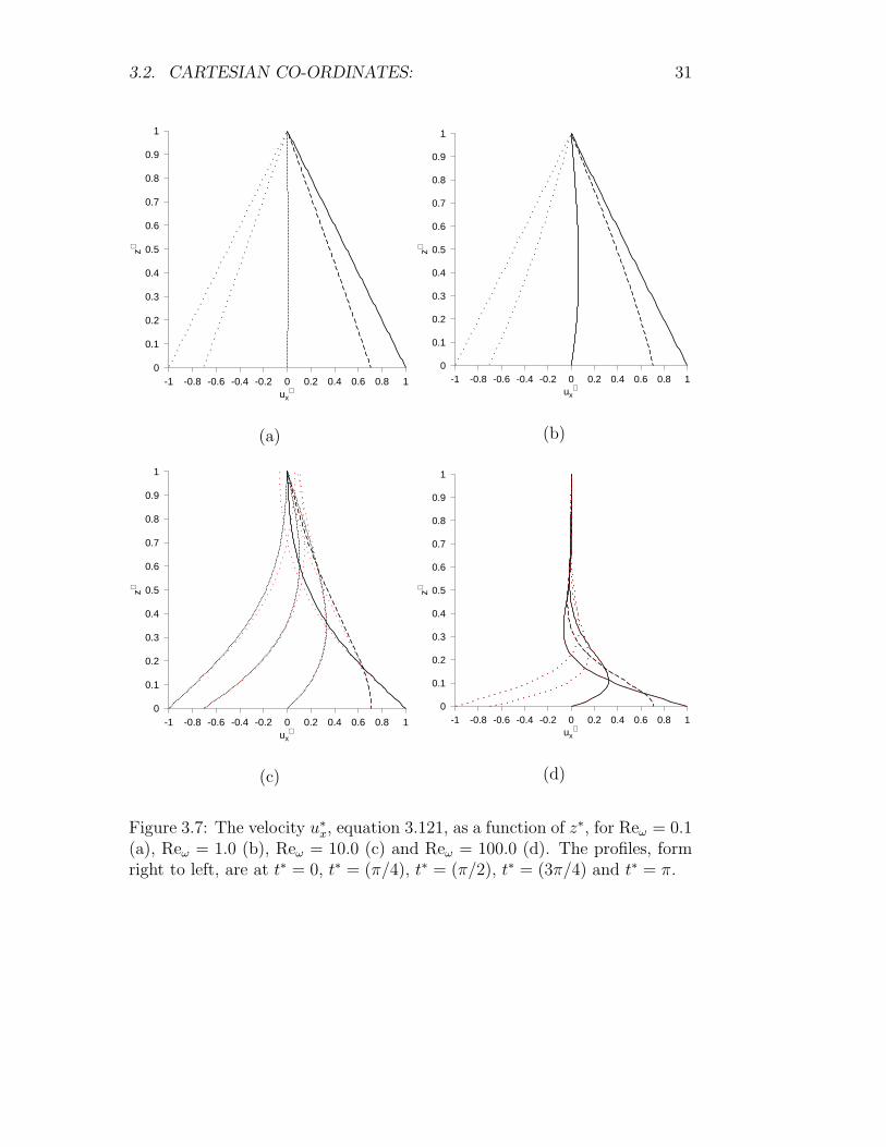
The numerical solutions for the velocity u∗x are shown as a function of z∗
in figure ?? for Reω = 0.1, 1.0, 10.0 and 100.0. It is clear that the velocity
3.2. CARTESIAN CO-ORDINATES: 31
-1 -0.8 -0.6 -0.4 -0.2 0 0.2 0.4 0.6 0.8 1ux
∗
0
0.1
0.2
0.3
0.4
0.5
0.6
0.7
0.8
0.9
1z∗
(a)
-1 -0.8 -0.6 -0.4 -0.2 0 0.2 0.4 0.6 0.8 1ux
∗
0
0.1
0.2
0.3
0.4
0.5
0.6
0.7
0.8
0.9
1
z∗
(b)
-1 -0.8 -0.6 -0.4 -0.2 0 0.2 0.4 0.6 0.8 1ux
∗
0
0.1
0.2
0.3
0.4
0.5
0.6
0.7
0.8
0.9
1
z∗
(c)
-1 -0.8 -0.6 -0.4 -0.2 0 0.2 0.4 0.6 0.8 1ux
∗
0
0.1
0.2
0.3
0.4
0.5
0.6
0.7
0.8
0.9
1
z∗
(d)
Figure 3.7: The velocity u∗x, equation 3.121, as a function of z∗, for Reω = 0.1
(a), Reω = 1.0 (b), Reω = 10.0 (c) and Reω = 100.0 (d). The profiles, formright to left, are at t∗ = 0, t∗ = (π/4), t∗ = (π/2), t∗ = (3π/4) and t∗ = π.

32 CHAPTER 3. TRANSPORT IN ONE AND TWO DIMENSIONS
profiles are nearly linear functions of z∗ for Reω = 0.1. In contrast, the fluidmotion is confined to a thin layer near the moving plate for Reω = 100.0,and there is almost no motion in the bulk of the fluid. The physical reasonfor this is as follows.
In the limit Reω → 0, the solution for the fluid velocity, 3.120, is
u∗x(z
∗) = (1 − z∗) cos (t∗) (3.122)
The physical reason for this result is as follows. The Reynolds number Reω
can be interpreted as the product of the frequency ω, and the time requiredfor the momentum to diffuse across the length of the channel, (H2/ν). ForReω ≪ 1, the time period (2π/ω) of variation of the velocity of the bottomplate is long compared to the time required for momentum to diffuse acrossthe channel. In this case, the velocity profile at any instant is the linear veloc-ity profile for a steady flow, in which the velocity at z∗ = 0 is (u∗
x = cos (t∗),the instanteneous velocity of the bottom plate at that instant. Therefore,we recover the linear profile for the steady flow between two plates, but withthe velocity amplitude varying in time proportional to cos (t∗).
In the limit ω∗ ≫ 1, the fluid velocity field is given by
u∗x(z
∗) = Real(exp (−√
ıReωz∗) exp (ıt∗))
= exp (−√
Reω/2z∗)(cos (√
Reω/2z∗) cos (t∗) − sin (√
Reω/2z∗) sin (t∗))(3.123)
In this case, the velocity field decreases over a distance z∗ ∼ (1/√
Reω/2) fromthe surface. This is because the frequency of oscillation is large comparedto the time required for diffusion of momentum across the channel, and themomentum diffuses only to a distance comparable to (H/
√Reω). Beyond
this distance, the momentum generated during the positive and negativeparts of a cycle cancel out, and the fluid velocity approaches zero. Thus, the‘penetration depth’ of the fluid velocity field is proportional to (H/
√Reω) in
the limit Reω ≫ 1.
3.3 Effect of bulk flow and reaction in mass
transfer
In this section, the special effects of bulk flow and reactions on the solutionsfor unidirection mass transfer problems are examined.
3.3. EFFECT OF BULK FLOW AND REACTION IN MASS TRANSFER33
g
v (x)z
z+ z∆
x
z
z=0
z=L
z
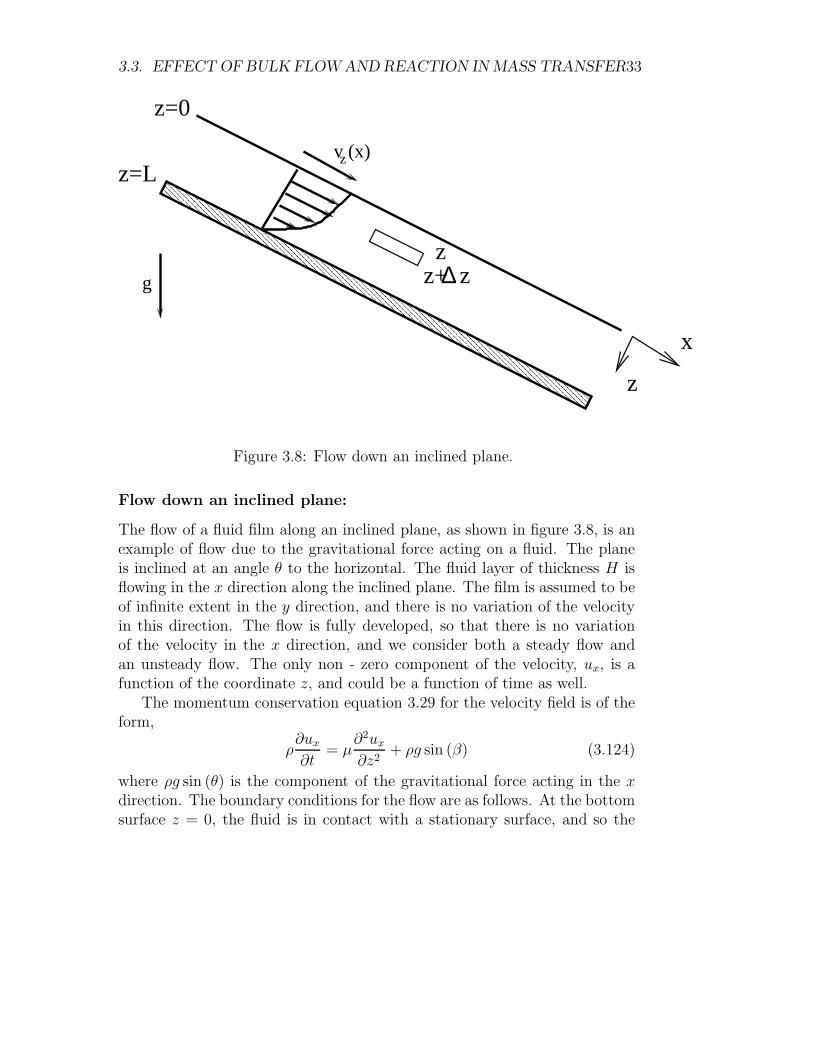
Figure 3.8: Flow down an inclined plane.
Flow down an inclined plane:
The flow of a fluid film along an inclined plane, as shown in figure 3.8, is anexample of flow due to the gravitational force acting on a fluid. The planeis inclined at an angle θ to the horizontal. The fluid layer of thickness H isflowing in the x direction along the inclined plane. The film is assumed to beof infinite extent in the y direction, and there is no variation of the velocityin this direction. The flow is fully developed, so that there is no variationof the velocity in the x direction, and we consider both a steady flow andan unsteady flow. The only non - zero component of the velocity, ux, is afunction of the coordinate z, and could be a function of time as well.
The momentum conservation equation 3.29 for the velocity field is of theform,
ρ∂ux
∂t= µ
∂2ux
∂z2+ ρg sin (β) (3.124)
where ρg sin (θ) is the component of the gravitational force acting in the xdirection. The boundary conditions for the flow are as follows. At the bottomsurface z = 0, the fluid is in contact with a stationary surface, and so the

34 CHAPTER 3. TRANSPORT IN ONE AND TWO DIMENSIONS
fluid velocity is zero at this surface.
ux = 0 at z = 0 (3.125)
At the top surface z = H , the liquid is in contact with a gas. Since thegas viscosity is small compared to the viscosity of the liquid, the shear stressexerted by the gas on the liquid is small. Therefore, we can use the ‘zeroshear stress’ condition at the top surface,
τxz = µ∂ux
∂z= 0 at z = H (3.126)
Thus, the gradient of the velocity in the z direction is zero at the free surface.The scaled z co-ordinate in equation 3.124 can be defined as z∗ = (z/H),
as before. How do we define a scaled velocity u∗x, since there is no prescribed
velocity at the boundaries? The scaling for the velocity can be determinedfrom the momentum conservation equation ?? itself, since this equation con-tains a ‘source’ of momentum due to the gravitational force. If we substitutez = z∗H , and divide the entire equation by ρg sin (θ), we obtain,
∂u∗x
∂t∗=
∂2u∗x
∂z∗2+ 1 (3.127)
where the scaled velocity u∗x = (µux/(H2ρg sin (θ))), and t∗ = (tν/H2) is the
scaled time. Equation 3.127 is a linear partial differential equation for u∗x,
which contains an inhomogeneous term, 1, due to the body force. In contrast,the boundary conditions for the scaled velocity u∗
x are both homogeneous,
u∗x = 0 at z∗ = 0 (3.128)
∂u∗x
∂z∗= 0 at z∗ = 1 (3.129)
Therefore, in the present problem, there is no forcing at the boundaries, andthe flow is driven by forcing within the flow itself due to the gravitationalflow. In contrast, in the flow between two flat plates in section ??, there is noforcing within the flow, and the flow is driven by the motion of the boundary.
At steady state, the time derivative in equation 3.127 is set equal to zero,
∂2u∗x
∂z∗2+ 1 = 0 (3.130)

3.3. EFFECT OF BULK FLOW AND REACTION IN MASS TRANSFER35
This solution of this equation, which satisfies the boundary conditions 3.128and 3.129, is,
u∗x = z∗ − z∗2
2(3.131)
The dimensional velocity can be easily determined from the above,
ux =ρg sin (θ)
µ
(
zH − z2
2
)
(3.132)
Various average quantities can be determined once this velocity profile isknown.
1. the maximum velocity, uxm, is clearly at x = 0
uxm =ρgH2 sin (θ)
2µ(3.133)
2. The total flow rate is determined from
Q =∫ H
0dz∫ W
0dyux
=ρgWH3 sin (θ)
3µ(3.134)
3. The mean velocity can be calculated from
ux =Q
h
=ρgWH2 sin (θ)
3µ(3.135)
4. The film thickness δ can be expressed in terms of the flow rate as
H =
(
3µQ
ρgW sin (θ)
)1/3
(3.136)
5. The total force on the inclined surface in the z direction is given by
F =∫ L
0dz∫ W
0dy τxz|x=h (3.137)
= ρghLW sin (θ) (3.138)
This is just equal to the weight of the fluid in the z direction understeady flow conditions.

36 CHAPTER 3. TRANSPORT IN ONE AND TWO DIMENSIONS
Next, we consider the start-up of the flow in an initially stationary filmof fluid down an inclined plane. The film is initially horizontal, and at t = 0,the film is inclined at an angle θ with respect to the horizontal. As before,there is no variation of the velocity in the streamwise x direction, but there isa flow development in time. The momentum conservation equation is 3.127,with boundary conditions 3.128 and 3.129. In addition, at the initial timet∗ = 0, the fluid is stationary, and so the initial condition is,
u∗x = 0 at t∗ = 0 for all z∗ > 0 (3.139)
The unsteady problem is solved by the method of separation of variables.First, the velocity is separated into two parts, the steady part u∗
xs and thetransient part u∗
xt,u∗
x = u∗xs + u∗
xt (3.140)
The equation for the steady velocity field, 3.130, is subtracted from the equa-tion for the total velocity field, 3.127, to obtain the equation for the transientpart of the velocity field.
∂u∗xt
∂t=
∂2u∗x
∂z∗2(3.141)
The boundary conditions for the total velocity and the steady velocity field,3.128 and 3.129, are both homogeneous, the boundary conditions for thetransient velocity field are also homogeneous,
u∗xt = 0 at z∗ = 0 (3.142)
∂u∗xt
∂z∗= 0 at z∗ = 1 (3.143)
Finally, the initial condition for u∗xt is obtained by subtracting the steady
solution u∗xs (equation 3.131) from the initial condition 3.139,
u∗xt = −(z∗ − (z∗2/2)) at t∗ = 0 for all z∗ (3.144)
As in the case of the transient flow in a channel in section ??, the transientpart of the velocity field has homogeneous boundary conditions, but theinitial condition is inhomogeneous.
The separation of variables procedure provides the following solution forthe transient part of the velocity field,
u∗xt =
∞∑
n=1
(Cn sin (αnz∗) + Dn sin (αnz
∗)) exp (−α2nt∗) (3.145)

3.3. EFFECT OF BULK FLOW AND REACTION IN MASS TRANSFER37
where the coefficients Cn, Dn and the eigenvalues αn are chosen so that theboundary conditions 3.142 and 3.143, and the initial condition 3.144, aresatisfied. The boundary condition 3.142 is satisfied only if Dn = 0, for alln, while the boundary condition 3.143 is satisfied if αn = (2n + 1)π/2 forn = 1, 2, . . .. Therefore, the solution for u∗
xt which satisfies the boundaryconditions at z∗ = 0 and z∗ = 1 is,
u∗xt =
∞∑
n=1
Cn sin ((2n + 1)πz∗/2) exp (−((2n + 1)/2)2π2t∗) (3.146)
The coefficients Cn determined from the initial condition at t∗ = 0, equa-tion 3.144.
u∗xt(z
∗, t∗ = 0) = −(z∗ − z∗2/2)
=∞∑
n=1
Cn sin ((2n + 1)πz∗/2) (3.147)
In the solution 3.147, the functions sin ((2n + 1)πz∗/2) form a set of basisfunctions which are orthogonal to each other. The orthogonality relation is,
∫ 1
0dz∗ sin ((2n + 1)πz∗/2) sin ((2m + 1)πz∗/2) =
δmn
2(3.148)
This orthogonality relation can be used to determine the coefficients Cn inequation 3.147,
∫ 1
0dz∗(−(z∗ − z∗2/2)) sin ((2m + 1)πz∗/2)
=∫ 1
0dz∗ sin ((2m + 1)πz∗/2)
∞∑
n=1
Cn sin ((2n + 1)πz∗/2)
= Cm/2 (3.149)
Thus, the coefficients Cm are,
Cm = − 1
π3((2n + 1)/2)3(3.150)
This, the final solution for the unsteady velocity field is,
u∗x = (z∗−z∗2/2)−
∞∑
n=1
(π3((2n+1)/2)3)−1 sin ((2n + 1)πz∗/2) exp (−((2n + 1)/2)2π2t∗)
(3.151)

38 CHAPTER 3. TRANSPORT IN ONE AND TWO DIMENSIONS
The above analytical results are valid only if the flow is laminar andthe streamlines are smooth, so that the flow can be considered steady. Theseconditions are satisfied for the slow viscous flow of a thin film. As the velocityincreases or the film thickness increases, it has been found that there is atransition from a laminar flow ith straight streamlines to a laminar flow withrippling and then to a turbulent flow. The conditions under which thesetransitions occur is determined by the ‘Reynolds number’, Re = (4ρhux/µ).A laminar flow without rippling is observed for Re < 10, while there isrippling for 10 < Re < 1000. The flow becomes turbulent when the Reynoldsnumber increases beyond about 1000.
3.3.1 Viscous heating in a channel:
There is a dissipation of energy during the shear flow of a viscous liquid dueto fluid friction, and this energy increases the temperature of the fluid. Weconsider the specific example of a pressure-driven flow in a channel betweentwo infinite flat plates located at z = 0 and z = H . The temperature atboth the bounding surfaces is T0, but there is an increase in the temperaturewithin the channel due to the heat generated by viscous dissipation. Wewould like to find out the temperature within the channel. At steady state,the velocity profile in the channel is given by,
ux = − 1
2µ
dp
dxz(H − z)
= 4U
(
z
H−(
z
H
)2)
(3.152)
where (dp/dx) is the pressure gradient, and U is the maximum velocity atthe center of the channel.
The rate of dissipation of energy due to fluid friction will be calculatedlater when we derive the mass, momentum and energy balance equations fora fluid. For a laminar shear flow where the velocity is in the x direction andthe velocity variation is in the z direction, the rate of dissipation of energy(per unit volume per unit time), Se in equation 3.15, is given by,
Se = τxydux
dz
= µ
(
dux
dz
)2
(3.153)

3.3. EFFECT OF BULK FLOW AND REACTION IN MASS TRANSFER39
where τxy is the shear stress, and (dux/dy) is the strain rate. Using thisvelocity profile in equation 3.152, we find that the dissipation rate per unitvolume, Se, is,
Se = 16U2
(
z
H−(
z
H
)2)2
(3.154)
At steady state, the energy balance equation, 3.19, reduces to,
kd2T
dz2+
16µU2
H2
(
1 − 2z
h
)2
= 0 (3.155)
The boundary conditions are,
T = T0 at z = 0 (3.156)
T = T0 at z = H (3.157)
It is natural to define a scaled z co-ordinate, z∗ = (z/H), and a scaledtemperature, T ∗ = ((T − T0)/T0). Defined this way, the scaled temperatureis the ratio of the local temperature rise due to viscous heating and the walltemperature. With this non-dimensionalisation, the energy balance equationbecomes,
d2T ∗
dz∗2+ 16Br(1 − 2z∗)2 = 0 (3.158)
with boundary conditions,
T ∗ = 0 at z∗ = 0 (3.159)
T ∗ = 0 at z∗ = 1 (3.160)
where the Brinkman number is,
Br =µU2
kT0
(3.161)
Equation 3.158 can be easily solved, subject to boundary conditions 3.159and 3.160, to obtain,
T ∗ = Br
(
8z∗(1 − z∗)(1 − 2z∗ + 2z∗2)
3
)
(3.162)
The profile of the scaled temperature, divided by Br, is shown as a functionof the scaled z co-ordinate in figure 3.3.1. The temperature profile is very

40 CHAPTER 3. TRANSPORT IN ONE AND TWO DIMENSIONS
0 0.1 0.2 0.3 0.4 0.5(T∗ /Br)
0
0.1
0.2
0.3
0.4
0.5
0.6
0.7
0.8
0.9
1
z∗
Figure 3.9: The ratio (T ∗/Br) of the scaled temperature T ∗ = ((T −T0)/T0),as a function of z∗ a channel.

3.3. EFFECT OF BULK FLOW AND REACTION IN MASS TRANSFER41
flat at the center of the channel, because the strain rate (dux/dz) decreasesto zero at the center, and the rate of generation also decreases to zero. Therate of generation of heat is a maximum near the wall, where the strain rateis a maximum.
From equation 3.162 for the temperature profile, the fractional increasein the temperature within the channel is given by the Brinkman number.For Br ≪ 1, the temperature rise in the channel is small compared to thewall temperature, and so change in temperature due to viscous heating canbe neglected. Viscous heating also results in a flux of energy across the wallof the channel, which is given by,
qz = −kdT
dz
= −kT0
H
dT ∗
dz∗
=8kT0(1 − 2z∗)3Br
3H
=8µU2(1 − 2z∗)3
3H(3.163)
The heat flux is negative at the bottom surface at z∗ = 0, because heat istransferred downwards from the fluid to the wall. At z∗ = 1, the heat flux ispositive because heat is transferred upwards to the wall. In both cases, themagnitude of the heat flux is given by (8µU2/3H).
Recall that in dimensional analysis of the heat transfer in a heat exchangerin chapter 1, we had assumed that there is no conversion of mechanical energyto heat energy. The present calculation shows that this assumption is validonly when the flux qz due to viscous heating, (8µU2/3H), is small comparedto the flux due to the temperature difference across the wall of the heatexchanger. When the heat flux due to viscous heating is comparable to thatdue to the temperature difference across the wall of the tube, it is necessaryto include the viscous heating in the energy balance equation, and the Nusseltnumber will be a function of the Brinkman number as well.
3.3.2 Diffusion with homogeneous reaction
A gaseous reactant A dissolves in a liquid B, and undergoes a first orderreaction A + B → AB, in a tank of height L, as shown in figure 3.10. Themass balance equation, ?? has to be modified in this case due to the presence

42 CHAPTER 3. TRANSPORT IN ONE AND TWO DIMENSIONS
of a ‘consumption’ term due to chemical reaction. The mass balance equationat steady state takes the form
jAz|z − jAz|z+∆z − kcAS∆z = 0 (3.164)
This can be reduced to a differential equation by dividing throughout byS∆z, and taking the limit ∆z → 0,
djAz
dz− kCA = 0 (3.165)
If the concentration of A is small, the flux of A is given by
jAz = −DABdcA
dz(3.166)
Inserting this into the concentration equation 3.165, we get
−DABd2cA
dz2+ kCA = 0 (3.167)
The boundary conditions are
cA = cA0 at z = 0
jAz = 0 at z = H (3.168)
The solution that satisfied both these conditions is
CA
CA0=
cosh ((kL2/DAB)1/2(1 − (z/L)))
cosh (kL2/DAB)1/2(3.169)
3.3.3 Diffusion in a stagnant film
Water evaporates from a container through a stagnant air film through aglass tube into dry air flowing at the top of the tube, as shown in figure 3.11.If the mole fraction at the surface of the liquid surface is the saturation molefraction xWs, and the dry air flowing past the tube does not contain anywater, what is the concentration profile of water in the glass tube?
Though the air in the tube is stationary, the mean velocity across anyhorizontal surface in the tube is not zero, because of the flow of water vapour

3.3. EFFECT OF BULK FLOW AND REACTION IN MASS TRANSFER43
z
z=0
z=L
zz+ z∆
c=c at z=0
j =0 at z=Lz
Figure 3.10: Diffison with homogeneous chemical reaction.

44 CHAPTER 3. TRANSPORT IN ONE AND TWO DIMENSIONS
Water
x
z
z=L
z=0
Dry air
Figure 3.11: Diffusion with bulk flow.

3.4. CYLINDRICAL CO-ORDINATES: 45
across the surface. The flux of water across a surface, jWz, contains a com-ponent due to the bulk flow, as well as a component due to the diffusion ofwater across the surface.
jWz = −cDWAdxW
dz+ xW (jWz + jAz) (3.170)
The last term on the right side of equation 3.170 is the flux of water dueto the bulk flow, where the total molar flow rate is the sum of the fluxes ofwater (jWz) and air (jAz). In this particular case, the flux of air is identicallyzero, and so the flux of water vapour across a surface is given by
jWz = − c
1 − xW
dxW
dz(3.171)
The mass balance equation is obtained by writing a flux balance across asection of thickness ∆z of the tube, which at steady state provides,
jWz|z+∆z − jWz|z = 0 (3.172)
If the above equation is divided by ∆z the differential equation for the fluxin the limit ∆z → 0 is
djWz
dz=
d
dz
(
1
1 − xW
dxW
dz
)
= 0 (3.173)
This equation is solved to obtain
− log (1 − xW ) = A1z + A2 (3.174)
The constants A1 and A2 are determined from the boundary conditions xW =xWs at z = 0 and x = 0 at z = l,
(1 − xW )
(1 − xWs)=
(
(1 − xWf )
(1 − xWs)
)z/l
(3.175)
3.4 Cylindrical co-ordinates:
3.4.1 Balance laws:
In the previous section, we had used a Cartesian co-ordinate system to anal-yse the transport between two flat plates. The Cartesian co-ordinate system

46 CHAPTER 3. TRANSPORT IN ONE AND TWO DIMENSIONS
was convenient for this geometry, because the boundaries were surfaces onwhich one of the co-ordinates (the z co-ordinate) is a constant. Due to this,the boundary conditions were applied at a constant value of z. In the caseof systems with cylindrical geometry, such as the flow through a pipe, heatconduction across the surface of a tube, or the mass transfer in a cylindri-cal pore on a catalyst surface, the use of a Cartesian co-ordinate system iscomplicated, because none of the co-ordinates is a constant on the cylindri-cal surface. It is more convenient to use a cylindrical co-ordinate system,as shown in figure 3.12. This co-ordinate system has cylindrical symmetryabout an ‘axis’, which is the z axis in figure 3.12. The co-ordinates in thecylindrical co-ordinate system are (r, θ, z), where r is the distance of a pointfrom the z axis, and θ is the angle between the position vector and the xco-ordinate. The third co-ordinate, z, is identical to that in a Cartesian co-ordinate system. In our analysis of unidirectional transport, we will assumethat there is variation of concentration, temperature or velocity only in ther direction and in time, and there is no dependence on θ and z.
First, we derive a heat balance equation for the temperature variation ina cylindrical shell of thickness ∆r and height ∆z at radius r. The terms inthe balance equation 3.11 for the energy in the cylindrical shell are as follows.
(
Accumulation of energyin the shell
)
= ρCp(T (x, y, z, t+∆t)−T (x, y, x, t))2πr∆r∆z
(3.176)The total energy entering the shell at r is the product of the heat flux, thesurface area, and the time interval ∆t,
(
Input ofenergy into shell
)
= − (qr(2πr∆z∆t))|r (3.177)
where qr is the heat flux in the radial direction. Similarly, the total energyleaving the shell at r + ∆r is
(
Output ofenergy from shell
)
= (qr(2πr∆z∆t))|r+∆r (3.178)
The source of energy in the differential volume is,
(
Source ofenergy from shell
)
= Se(2πr∆r∆z∆t) (3.179)

3.4. CYLINDRICAL CO-ORDINATES: 47
r
z
∆z
R
∆ r r T*=0
Figure 3.12: Heat diffusion into a cylinder.

48 CHAPTER 3. TRANSPORT IN ONE AND TWO DIMENSIONS
where Se is the amount of energy generated per unit volume per unit time.When these are inserted into the conservation equation 3.11, and divided by2πr∆r∆z∆t, the net energy balance for the shell is
ρCp(T (x, y, z, t + ∆t) − T (x, y, x, t))
∆t=
1
r∆r
(
(rqr)|r − (rqr)|r+∆r
)
+ Se
(3.180)Taking the limit ∆r → 0 and ∆t → 0, the partial differential equation forthe temperature field is
ρCp∂T
∂t= −1
r
∂
∂r(rqr) + Se (3.181)
The heat flux qr is related to the temperature gradient in the radial directionby the Fourier’s law for heat conduction,
qr = −k∂T
∂r(3.182)
With this, the energy balance equation becomes,
ρCp∂T
∂t=
1
r
∂
∂r
(
rk∂T
∂r
)
+ Se (3.183)
When the thermal conductivity is independent of position, the energy balanceequation reduces to,
∂T
∂t= α
1
r
∂
∂r
(
r∂T
∂r
)
+ (Se/ρCp) (3.184)
where α = (k/ρCp) is the thermal diffusivity.It is important to note that there is a variation in the surface area of the
shell as r varies. This leads to a more complicated form for the diffusionterm in 3.184, in comparison to the second derivative with respect to z inthe diffusion from a flat plane, 3.20.
Similar to equation 3.184, the mass conservation equation for a cylindricalco-ordinate system, analogous to equation 3.10 for a Cartesian co-ordinatesystem, is,
∂c
∂t= D
1
r
∂
∂r
(
r∂c
∂r
)
+ S (3.185)
where D is the mass diffusivity and S is the rate of increase of mass per unitvolume per unit time.

3.4. CYLINDRICAL CO-ORDINATES: 49
In section ??, the momentum conservation equation was written for thevelocity ux, which is a constant in the x direction, but is a function of thedirection z between the two plates. In a cylindrical co-ordinate system, thereare two velocity components perpendicular to r, the θ co-ordinate uθ and thez co-ordinate uz. Momentum balance equations could be written in eitherof these two directions. A momentum balance equation in the z directionis solved when there is a flow along the axis of the cylindrical co-ordinatesystem, such as the flow in a pipe. The velocity uθ is non-zero when thereis a flow around the axis of the cylindrical co-ordinate system, with circularstreamlines. The momentum balance for uθ is similar to the energy and massbalance equations 3.184 and 3.185,
ρ∂uθ
∂t= µ
1
r
∂
∂r
(
r∂uθ
∂r
)
+ fθ (3.186)
where fθ is the force per unit volume acting in the θ direction.
3.4.2 Heat transfer across the wall of a pipe:
Consider a cylindrical pipe with inner radius Ri and outer radius Ro, asshown in figure ??. The inner surface is at temperature Ti, while the outersurface is at temperature To. We would like to determine the heat flux acrossthe wall of the pipe, which has thermal conductivity k at steady state.
The scaled temperature and distance are defined as T ∗ = (T−Ti)/(To−Ti)and r∗ = (r/Ri). The heat balance equation at steady state is,
1
r∗∂
∂r∗
(
r∗∂T ∗
∂r∗
)
= 0 (3.187)
and the boundary conditions are,
T ∗ = 0 at r∗ = 1 (3.188)
T ∗ = 1 at r∗ = (Ro/Ri) (3.189)
This can be easily solved to obtain,
T ∗ =log (r∗)
log (Ro/Ri)(3.190)

50 CHAPTER 3. TRANSPORT IN ONE AND TWO DIMENSIONS
Thus, we obtain a logarithmic variation in the temperature along the radiusof the tube. The heat flux, qr, is given by,
qr = −k∂T
∂r
= −k(To − Ti)
Ri
∂T ∗
∂r∗
= − k(To − Ti)
r∗Ri log (Ro/Ri)(3.191)
The total heat transfer rate across the tube wall (per unit length of the tube)is obtained by integrating the heat flux over the surface. At which surfaceshould this be calculated, the inner surface, the outer surface or somewherein between? The answer is that it does not matter which surface we use, theheat transfer rate is independent of the radius of the surface. This is becausein the conservation equation 3.187, there is no generation or consumptionof heat in the tube wall, and the temperature is at steady state. Therefore,the heat transferred per unit time is the same across any cylindrical surfacein the wall of the tube. If we consider a cylindrical surface of radius r andlength L, the heat transferred across this surface per unit time, Q, is (2πrL)times the heat flux,
Q = (2πrL) ×(
− k(To − Ti)
r∗Ri log (Ro/Ri)
)
=2πk(To − Ti)L
log (Ro/Ri)(3.192)
It is convenient to define an ‘average’ radial heat flux based on the thicknessof the tube wall, (Ro − Ri),
qr =Q
2πL(Ro − Ri)(3.193)
Based on this definition, the average heat flux from equation 3.192 is,
qr = − k(To − Ti)
(Ro − Ri) log (Ro/Ri)(3.194)

3.4. CYLINDRICAL CO-ORDINATES: 51
3.4.3 Heat conduction from a wire:
In our discussion of heat conduction into an infinite medium in a Cartesianco-ordinate system, a similarity solution was used because there are no lengthand time scales in the problem. Such a solution cannot be used for the con-duction from a cylinder into an infinite medium, because the radius of thecylinder also provides a length scale which can be used to non-dimensionalisedistances. However, there is one special situation where the similarity solu-tion procedure can be used, which is the heat conduction from a thin wire.This problem is of relevance in real applications, because resistance heatingis a common method for heating fluids. The problem is as follows.
A resistance heating appratus for a fluid consists of a thin wire immersedin a fluid. In order to design the appratus, it is necessary to determine thetemperature in the fluid as a function of he heat flux from the wire. For thepurposes of the calculation, the wire can be considered of infinite length sothat the heat conduction problem is effectively a two dimensional problem.In addition, the thickness of the wire is considered small compared to anyother length scales in the problem, so that the wire is a line source of heat.The wire and the fluid are initially at a temperature T0. At time t = 0, thecurrent is switched on so that the wire acts as a source of heat, and the heattransmitted per unit length of the wire is Q. The thermal conductivity ofthe liquid is K.
There is an important difference between the above problem and theproblem of conduction into an infintite medium in Cartesian co-ordinates.In the latter, the temperature at the surface was instanteneously increasedto from T0 to T1 at time t = 0. In the above problem, we have specified theheat produced per unit length of the wire, Q. This is because the thicknessof the wire is small compared to any other length scales, and we take thelimit where the radius of the wire goes to zero. (As indicated above, if theradius of the wire is finite, it is possible to scale all lengths by the radiusof the wire, and a similarity solution cannot be used). As the thicknessgoes to zero, the surface area of the wire goes to zero, and so the heat flux(ratio of heat generated and surface area) will go to infinity. An infiniteheat flux implies an infinite temperature gradient, and so it is not possible tospecify the temperature itself at the surface of the wire. Rather than usinga boundary condition at the surface, we will use the condition that the totalheat generated per unit length is Q in order to determine the constants inthe solution.

52 CHAPTER 3. TRANSPORT IN ONE AND TWO DIMENSIONS
The scaled temperature is defined as T ∗ = ((T − T∞)/T∞), so that thescaled temperature is zero in the limit r → ∞. The heat conduction equationin the fluid is,
∂T ∗
∂t= α
(
1
r
d
drrdT ∗
dr
)
(3.195)
One of the boundary conditions are that T ∗ → 0 in the limit r → ∞. Theother boundary condition is a flux condition. The total heat transmitted, perunit length, of the wire is Q. Therefore, the flux from a cylindrical surface ofradius r is Q/(2πr). Therefore, the requirement at the wire surface, in thelimit r → 0, is that
−KT∞dT ∗
dr=
Q
2πr(3.196)
where Q is a constant.To solve for the temperature field, note that there is no length scale in
the problem (the wire is infinitesimal in thickness, and the boundaries areat infinity). Therefore, a similarity solution can be used with the similar-ity variable ξ = (r/
√αt). The heat conduction equation, in terms of this
variable, isd2T ∗
dξ2+
(
1
ξ+
ξ
2
)
dT ∗
dξ= 0 (3.197)
This equation can be solved to obtain the
dT ∗
dξ=
C
ξexp (−ξ2/4) (3.198)
The temperature can be obtained by integrating the above equation withrespect to ξ, and realising that T = 0 as ξ → ∞.
T ∗ =∫ ξ
∞dξ′
C
ξ′exp (−ξ′2/4) (3.199)
The above equation shows that the temperature at the surface of the wire isundefined, because the integral in equation 3.199 increases proportional tolog (ξ) as ξ → ∞. This was anticipated when we framed the problem, wherewe defined the total heat generated per unit length of the wire, and not thetemperature at the wire itself.
The constant C can be determined from the flux condition, in the limitr → 0(ξ → 0),
KdT ∗
dr= − Q
2πr(3.200)

3.4. CYLINDRICAL CO-ORDINATES: 53
When expressed in terms of ξ, this is equivalent to
dT ∗
dξ= − Q
2πKξ(3.201)
Substituting solution 3.198 into the above equation, we find that the constantC = (Q/2πK). Therefore, the solution for the temperature field is,
T ∗ =Q
2πk
∫ ξ
∞dξ′
1
ξ′exp (−ξ′2/4) (3.202)
The solution (T ∗/(Q/2πk)) is shown as a function of (r/√
αt) in figure ??.
3.4.4 Heat conduction into a cylinder:
A cylindrical container of radius R containing fluid with temperature T1 isdipped into a bath at temperature T0. Assume that the bath is large enoughthat the conduction of heat into the fluid does not appreciably change thetemperature of the bath, and that there is no resistance to heat transfer in thewalls of the container. The temperature in the cylinder is to be determinedas a function of time and position is to be determined.
The conservation equation 3.184 can be scaled as follows. The scaledradius and time are defined as r∗ = (r/R) and t∗ = (tR2/α), since R is thelength scale in the radial direction. The scaled temperature is defined as,T ∗ = (T − T0)/(T1 − T0). The conservation equation 3.184, expressed inthese coordinates, is
∂T ∗
∂t∗=
1
r∗∂
∂r∗
(
r∗∂T ∗
∂r∗
)
(3.203)
since there is no heat generation within the cylinder.The boundary condition at the surface of the cylinder, r∗ = 1, is,
T ∗ = 0at r∗ = 1 for all t∗ (3.204)
At the center of the cylinder r∗ = 0, we specify a ‘symmetry condition’,that the temperature gradient, (∂T ∗/∂r∗) = 0. The reason for this is asfollows. Consider a section of the cylinder through a plane passing throughthe axis, as shown in figure ?? Since the temperature field is axisymmetric,the temperature is the same at equal distances on the right and left of theaxis. If the derivative (∂T ∗/∂r∗) is not zero, then the slope of the temperature

54 CHAPTER 3. TRANSPORT IN ONE AND TWO DIMENSIONS
profile at the axis from the left will be the opposite of the slope from theright, and so the slope at the center will not be uniquely defined. There isa discontinuity in the slope when the axis is approached from left and right.The slope will be continuous only if (∂T ∗/∂r∗) = 0 at r∗ = 0. Therefore,symmetry requires that
∂T ∗
∂r∗= 0at r∗ = 0 for all t∗(3.205)
At time t∗ = 0, the temperature is T0 throughout the cylinder except at thecylinder wall, and so the initial condition is,
T ∗ = 1 at t∗ = 0 for all r∗ < 1 (3.206)
The spatial boundary conditions at r∗ = 1 and r∗ = 0, equations 3.204and 3.205, both homogeneous, whereas the initial condition 3.206 is inho-mogeneous. As we had discussed in relation to the separation of variablesin Cartesian co-ordinates, the separation of variables procedure provides adiscrete set of eigenvalues and basis functions only if we have homogeneousboundary conditions in the spatial co-ordinates. Equations 3.204 and 3.205provide the required homogeneous boundary conditions in the present prob-lem.
Equation ?? is solved using the method of separation of variables. Thefinal steady state solution is one in which the temperature is uniform, T ∗ = 0,throughout the cylinder. The unsteady solution is solved using the substitu-tion
T ∗ = R(r∗)T (t∗) (3.207)
where R is a function of the radial coordinate, and T is a function of time.The form 3.207 is inserted into the temperature equation, 3.203, and theresulting equation is divided by R(r∗)T (t∗) to obtain
1
T∂T∂t∗
=1
R1
r∗∂
∂r∗
(
r∗∂R∂r∗
)
(3.208)
The left side of the above equation is only a function of time, while the rightside is only a function of r∗. Therefore, the equality can only be satisfiedif both sides are equal to constants. From our earlier experience of theseparation of variables in Cartesian co-ordinates, we know that this constant

3.4. CYLINDRICAL CO-ORDINATES: 55
has to be negative, so that the function T (t∗) decreases to zero in the limitt∗ → ∞. The right side of the above equation is first solved,
1
R
(
d2Rdr∗2
+1
r∗dRdr∗
)
= −β2 (3.209)
The solution for equation 3.199 can be obtained by recasting the equation as
r∗2 d2Rdr∗2
+ r∗dRdr∗
+ β2r∗R = 0 (3.210)
The two linearly independent solutions of the above equation 3.210, arespecial functions called ‘Bessel functions’, The Bessel functions Jn(x) andYn(x), are linearly independent solutions of the equation,
x2 d2y
dx2+ x
dy
dx+ (x2 − n2)y = 0 (3.211)
In equation 3.210, if we substitute x = βr∗, we find that the equation reducesto,
x2 d2Rdx2
+ xdRdx
+ x2R = 0 (3.212)
The solutions to this equation are ‘zeroeth order’ Bessel functions, with n =0,
R = C1J0(αr∗) + C2Y0(βr∗) (3.213)
There is no analytical solutions for these functions, and it is necessary toevaluate these numerically. The Bessel functions J0(x) and Y0(x) are shownas a function of x in figure 3.4.4. The Bessel functions have an oscillatorydependence on x, but the maximum amplitude of the oscillations decreasesand the period increases as x increases. The Bessel function J0(x) has amaximum value of 1 at x = 0. The Bessel function Y0(x) goes to −∞ forx → 0.
The values of the constants C1 and C2 are determined from the boundaryconditions at r∗ = 0 and r∗ = 1. From equation 3.205, (dR/dr∗) = 0 atr∗ = 0. From figure 3.4.4, it is observed that the derivative of J0(x) iszero, whereas the radial derivative of Y0(x) approaches infinity for r∗ → 0.Therefore, the boundary condition at r∗ = 0 can be satisfied only if C2 = 0.
The second boundary condition, T ∗ = 0 at r∗ = 1, is used to determinethe value of β in equation ??,
J0(β) = 0 (3.214)

56 CHAPTER 3. TRANSPORT IN ONE AND TWO DIMENSIONS
0 1 2 3 4 5 6 7 8 9 10x
-2
-1
0
1
J 0(x
), Y
0(x)
Figure 3.13: The Bessel functions, J0(x) and Y0(x) as a function of x.

3.4. CYLINDRICAL CO-ORDINATES: 57
Since J0(β) is an oscillatory function of β, there are multiple solutions forequation 3.214, which are the points where J0(x) crosses zero in figure 3.4.4.The first few solutions are, β1 = 2.40483, β2 = 5.52008, β3 = 8.65373,β4 = 11.79150 and β5 = 14.93090. Thus, the requirement that R(r∗) = 0 atr∗ = 1 results in a discrete set values for the ‘eigenvalue’ βn. This is analogousto the discrete values of βn = (nπ) in the unsteady heat conduction betweentwo parallel plates in section ??.
The equation for T ,1
TdTdt∗
= −β2n (3.215)
can be solved to obtainT = exp (−α2
nt∗) (3.216)
With this, the solution for the temperature field is
T ∗ =∞∑
n=1
AnJ0(βnr∗) exp (−β2nt∗) (3.217)
The coefficients An in equation 3.217 are chosen to satisfy the initialcondition at t∗ = 0,
∞∑
n=1
AnJ0(βnr∗) = 1 (3.218)
The values of the coefficients can be determined using orthogonality condi-tions for the Bessel functions, which in this case are
∫ 1
0r∗dr∗J0(βnr
∗)J0(βmr∗) =1
2(J1(βn))2 for m = n
= 0 for m 6= n (3.219)
In order to determine the coefficients, the right and left sides of 3.199 aremultiplied by r∗J0(βmr∗), and integrated from r∗ = 0 to r∗ = 1, to obtain
1
2(J1(βn))2An =
∫ 1
0r∗dr∗J0(βnr∗)
=J1(βn)
βn(3.220)
This provides the solution for An,
An =2
βnJ1(βn)(3.221)

58 CHAPTER 3. TRANSPORT IN ONE AND TWO DIMENSIONS
This, the final solution for the temperature field is,
T ∗ =∞∑
n=0
2
βnJ1(βn)J0(βnr∗) exp (−β2
nt∗) (3.222)
When we had solved the unsteady temperature profile in between twoflat plates in section ??, we had expressed the solution in terms of ‘basisfunctions’ Ψn = sin (nπz∗). In the present problems, the basis functions are,
Ψn = J0(βnr∗) (3.223)
where βn are the solutions of equation 3.214. The inner product, equivalentof equation 3.100, is,
〈Ψn, Ψm〉 =∫
x dx J0(βnx)J0(βmx) (3.224)
The orthogonality relation, equivalent to equation 3.101, is,
〈Ψn, Ψm〉 =J1(βm)δmn
2(3.225)
In the equivalent mass transfer problem, a cylinder of radius with uniformconcentration c = c1 is immersed into a fluid with concentration c = c0
at time t = 0, and it is necessary to find the variation of concentrationwith time in the cylinder. The scaled concentration field is defined as c∗ =(c − c0)/(c1 − c0). The concentration equation is identical to 3.222, withc∗ substituted for T ∗, and t∗ = (tD/R2), where D is the mass diffusioncoefficient.
In the equivalent momentum transfer problem, a fluid in a cylindricalcontainer is rotating with constant velocity uθ = rΩ. At t = 0, the wall ofthe container at r = R is instanteneously brought to rest, uθ = 0. We wouldlike to find out the velocity profile within the cylinder. The scaled velocityfield is defined as u∗
θ = (uθ/rΩ).

3.5. EFFECT OF PRESSURE ON MOMENTUM TRANSPORT 59
3.5 Effect of pressure on momentum trans-
port
The momentum balance condition states that the rate of change of momen-tum is equal to the applied force.
[
Rate ofmomentum in
]
−[
Rate ofmomentum out
]
+
[
Sum of forcesacting on the system
]
= 0
(3.226)This balance equation is written for a control volume of fluid which is in theform of a thin shell. Momentum enters or leaves the control volume due tofluid flow into or out of the control volume, or due to the stresses acting onthe surface due to viscosity. The forces acting on the system are usually thegravitational force or the centrifugal force. Momentum balances are usuallyeasy to apply only if the streamlines are straight. Applying momentumbalances to systems with curved streamlines is more difficult, as we shall seein the last example of this section.
The procedure for solving problems with momentum balance is to writethe momentum balance equation for a shell of finite thickness, and thenlet the thickness go to zero. In this limit, the difference equations for thevelocity field across a finite shell reduces to differential equations for thevelocity fields. These can then be solved, subject to appropriate boundaryconditions, in order to determine the velocity fields.
The boundary conditions generally involve specifying the velocity or stressfields at the boundaries of the flow. These conditions depend on the surfaceadjoining the liquid at its boundaries.
1. If there is a solid surface adjacent to the fluid, the appropriate boundarycondition is the ‘no slip’ condition which states that the velocity of thefluid at the surface is equal to the velocity of the surface itself.
2. At a liquid - gas interface, the momentum flux, and consequently thevelocity gradient, in the liquid side is assumed to be zero, because theviscosity of the gas is small compared to that of the liquid.
3. At a liquid - liquid interface, the momentum flux and the velocity arecontinuous across the interface.

60 CHAPTER 3. TRANSPORT IN ONE AND TWO DIMENSIONS
r
x
∆x
∆ rrR
Figure 3.14: Flow in a circular tube.
3.5.1 Flow through a pipe:
The flow through a circular tube is often encountered in engineering applica-tions, and the laminar flow can be analysed using shell momentum balances.The cylindrical coordinate system that is used for the analysis is shown infigure 3.14.
Consider a cylindrical shell of thickness ∆r and length ∆x. The balanceequation for the x component of the momentum can be written as,
Rate of changeof x momentum
= Sum of forces l (3.227)
The rate of change of momentum in a time interval ∆t within the differentialvolume under consideration can be written as,
Rate of changeof x momentum
=∆(ρux)
∆t(2πr∆r∆z (3.228)
where ∆(ρux) is the change in the momentum per unit volume in the timeinterval ∆t.
There are four bounding surfaces for the differential volume under con-sideration, two or which are at perpendicular to the x axis and located atx and x + ∆x, and two of which are perpendicular to the radial co-ordinateand are located at r and r + ∆r. The forces acting on the surfaces at x andx + ∆x can be separated into two parts, the first due to the pressure actingon the surfaces, and the second due to the flux of momentum due to fluid
3.5. EFFECT OF PRESSURE ON MOMENTUM TRANSPORT 61
motion. The forces due to fluid pressure can be written as,
Force due to pressureon surface at x
= p(r, θ, x)(2πr∆r)
Force due to pressureon surface at x + ∆x
= −p(r, θ, x + ∆x)(2πr∆r) (3.229)
Note that there is a negative sign for the force at x+∆x, because the pressurealways acts along the inward unit normal at the surface, and the inward unitnormal at x + ∆x is in the negative x direction. There is an additional forcedue to the flow of momentum into the differential volume through the surfaceat x and the flow of momentum out of the differential volume through thesurface at x + ∆x. This force is given by the product of the momentum flux(momentum transported per unit area per unit time) and the surface area.The momentum flux is the product of the momentum density (ρux) (per unitvolume) and the normal velocity to the surface ux. This is analogous to themass flux, which is the product of the concentration (mass density) c andthe normal velocity. Therefore, the force due to the flow of momentum is,
Force due to momentum flowon surface at x
= ((ρux)ux(2πr∆r)
Force due to momentum flowon surface at x + ∆x
= −p(r, θ, x + ∆x)(2πr∆r)(3.230)
Note that the force at (x + ∆x) is negative, since momentum leaves thedifferential volume at this surface. We can now add up all the contributionsto get
−2πrLτrz|r+2πrLτrz|r+∆r+2πr∆rρv2z
∣
∣
∣
z=0−2πr∆rρv2
z
∣
∣
∣
z=L+2πr∆rLρg+2πr∆r(p(r, x, t)−p(r, x+∆x, t))
(3.231)Since the fluid is considered to be incompressible, vz is equal at z = 0 andz = L. Therefore, the momentum flux due to fluid motion cancels out, andwe can divide by 2πL∆r and take the limit ∆r → 0 to get
ρ∂ux
∂t=
1
r
∂(rτrz)
∂r− ∂p
∂x(3.232)
Using Newton’s law of viscosity, τzr = µ(∂uz/∂r), we obtain the momentumconservation equation,
ρ∂uz
∂t= −∂p
∂z+ µ
1
r
∂
∂r
(
r∂uz
∂r
)
(3.233)

62 CHAPTER 3. TRANSPORT IN ONE AND TWO DIMENSIONS
Steady flow:
At steady state, the momentum conservation equation in the pipe reducesto,
−∂p
∂z+ µ
1
r
∂
∂r
(
r∂uz
∂r
)
(3.234)
The boundary conditions are the no-slip condition at the wall of the pipe(r = R),
uz = 0 at r = R (3.235)
and the symmetry condition at the axis of the tube,
∂uz
∂r= 0 at r = 0 (3.236)
The above equation can be integrated quite easily of the pressure is inde-pendent of r (no pressure variation in the radial direction). We will seelater, when we derive the momentum balance equation in the r direction,that the pressure variation in the r diretion is, indeed, zero, when there isno radial velocity ur. Physically, the reasoning is as follows. Just as theaxial momentum balance equation 3.233 balances the shear stresses (due tothe variation of uz in the radial direction), the acceleration term on the left(due to the time derivative of uz on the left) and the axial pressure gradient,the radial momentum balance equation will balance the stresses in the radialdirection (due to the variation of ur in the radial and axial directions), theacceleration term (due to the time derivative of ur) and the radial pressuregradient. However, ur is identically zero throughout the pipe, because flowis only in the axial (z) direction. Therefore, the pressure is invariant in theradial direction, and (∂p/∂r) = 0.
Since the pressure is only a function of z, equation 3.234 can be integratedto obtain,
uz =r2
4µ
∂p
∂z+ C1 log (r) + C2 (3.237)
The boundary condition 3.236 is satisfied only if C1 = 0, and C2 = −(R2/4µ)∂p∂z
from boundary condition 3.235. Therefore, the final expression for the veloc-ity field is,
uz = − 1
4µ
∂p
∂z(R2 − r2) (3.238)

3.5. EFFECT OF PRESSURE ON MOMENTUM TRANSPORT 63
This is the familiar parabolic velocity profile for the flow in a tube, calledthe Hagen-Poiseuille flow. Note that the velocity is positive when the pres-sure gradient is negative, that is, when the pressure decreases along the zdirection. The maximum value of the velocity at the center of the tube is,
umax = −R2
4µ
∂p
∂z(3.239)
The velocity profile 3.238 can also be expressed in terms of the maximumvelocity as,
uz = umax
(
1 −(
r
R
)2)
(3.240)
The shear stress is,
τzr = µ∂uz
∂r
= −2µumaxr
R2(3.241)
The shear stress is zero at the center of the tube, and it increases linearlywith radius. At the wall, the wall shear stress is given by,
τzr|r=R = −2µumax
R(3.242)
Note that the above shear stress is negative because it is the force per unitarea at a surface whose outward unit normal is in the radial direction. At thewall, this represents the force per unit area exerted on the fluid by the wall,which is in the −z direction. There is a force of equal magnitude exertedby the fluid on the wall, which is in the +z direction in accordance withNewton’s third law.
The volumetric flow rate is the product of the flow velocit and the cross-sectional area of the tube. In this case, the velocity is varying in the rdirection, and so it is necessary to integrate the velocity vz(r) times thedifferential area of a circular strip, (2πrdr) (figure ??) from r = 0 to r = R.
Q =∫ R
0uz2πr dr
−πR4
8µ
∂p
∂z(3.243)

64 CHAPTER 3. TRANSPORT IN ONE AND TWO DIMENSIONS
The average velocity u is defined as the ratio of the flow rate Q and thecross-sectional area (πR2),
u =Q
πR2= −R2
8µ
∂p
∂z(3.244)
The maximum velocity equation 3.240 is two times the average velocity 3.244,
umax = 2u (3.245)
The friction factor for the flow through a pipe is defined as the ratio ofthe wall shear stress and (ρu2/2),
f =τrz|r=R
(ρu2/2)(3.246)
Using equation 3.242 for the wall shear stress, we find that the friction factoris,
f =2µumax
R(ρu2/2)(3.247)
Using equation 3.245 for the relation between umax and u, we find that thefriction factor is,
f =16µ
ρumaxR=
16
Re(3.248)
where Re = (ρumaxR/µ), the Reynolds number based on the maximum fluidvelocity and the radius of the tube. The Reynolds number can also be ex-pressed as Re = (ρuD/µ), which is the Reynolds number based on the aver-age velocity and the tube diameter, because u = (umax/2) and D = 2R.
The friction factor correlation 3.248 is valid only when the flow in thetube is in the laminar regime, that is, when the Reynolds number is lessthan 2100. When the Reynolds number increases beyond 2100, there is aspontaneous transition to a turbulent flow, in which the friction factor issignificantly higher than that in a laminar flow. The solution 3.248 for alaminar flow is a valid solution for the momentum balance equation evenwhen the Reynolds number is higher than 2100. However, this solution be-comes unstable when the Reynolds number is higher than 2100, and naturallyoccuring disturbances in the flow cause a spontaneous transition to a morecomplicated ‘turbulent’ velocity profile. The distinction between the two isas follows. In the laminar flow, the streamlines within the flow are straight

3.5. EFFECT OF PRESSURE ON MOMENTUM TRANSPORT 65
and parallel to each other, and there is no motion in the cross-stream direc-ton. The transport of momentum in the cross-stream (radial) direction isby momentum diffusion, caused by the fluctuating velocity of the molecules.We had discussed this mechanism in detail in chapter 2. In contrast, in aturbulent flow, there are significant velocity fluctuations in both the stream-wise and the cross-stream directions, though the cross-stream velocity is zeroon average. The momentum transport is caused by the motion of correlatedregions within the fluid called ‘eddies’. This mechanism of momentum trans-port is more efficient than the molecular mechanism, and so this results in ahigher friction factor than that in a laminar flow. Due to this efficient cross-stream momentum transport, the velocity profile in a turbulent flow is alsomuch flatter and plug-like than the parabolic velocity profile in a laminarflow.
Oscillatory flow in a pipe
Oscillatory flows in tubes are of practical importance in physiological fluiddynamics, where the pumping of the heart causes a periodic variation inthe flow velocity along the arteries. Here, we study the simple exampleof the velocity profile due to an oscillatory pressure gradient, (δp/δz) =p cos (ωt). However, the solution procedure can be used for a more generaltime-periodic variation with frequency ω, because any periodic modulationcan be expressed as a sum of sine waves with frequencies that are integermultiples of ω.
We consider an unsteady (time-periodic) but fully developed flow alongthe tube, where the velocity is dependent on time but is independent of thez co-ordinate. The momentum conservation equation 3.233 for the presentcase is,
ρ∂uz
∂t=
µ
r
∂
∂r
(
r∂uz
∂r
)
− K cos (ωt) (3.249)
The boundary conditions at the center and the wall of the tube are the sameas those for a steady flow, 3.235 and 3.236. It is natural to define a scaledradial co-ordinate as r∗ = (r/R). The scaled time can be defined as t∗ = (ωt),since ω is the frequency of the pressure wave. How do we scale the velocityuz? It is clear that the magnitude of the velocity is related to K, which isthe amplitude of the pressure fluctuations. Therefore, we express equation
66 CHAPTER 3. TRANSPORT IN ONE AND TWO DIMENSIONS
3.249 in terms of r∗ and t∗, and divide throughout by K, to obtain,
ρω
K
∂uz
∂t∗=
µ
KR2
1
r∗∂
∂r∗
(
r∗∂uz
∂r∗
)
− cos (t∗) (3.250)
It is clear that all terms in the above equation are dimensionless, and there-fore, we can define a scaled velocity either as u∗
z = (µuz/KR2), or as u∗z =
(ρωuz/K). The former is obtained by balancing the viscous and pressureforces, and is appropriate for low Reynolds numbers where inertial forces arenegligible. The latter is obtained by balancing inertial and pressure forces,and is appropriate when the Reynolds number is large so that viscous forcesare negligible. We will proceed using the scaling obtained by balancing theviscous and pressure forces, and return later to consider the situation whenthe Reynolds number is large. Using a scaled velocity u∗
z = (µuz/KR2),equation 3.250 becomes,
Reω∂u∗
z
∂t∗=
1
r∗∂
∂r∗
(
r∗∂u∗
z
∂r∗
)
− cos (t∗) (3.251)
where Reω = (ρωR2/µ) is the Reynolds number based on the frequency ofoscillations and the tube radius.
As in the case of an oscillatory flow past a flat plate in section ??, it ismore convenient to solve the equation 3.251 with an inhomogenous term ofthe form exp (ıt), and then take the real part of this to obtain the solutionfor u∗
z. Therefore, we define a complex velocity field u†z as the solution of the
equation,
Reω∂u†
z
∂t∗=
1
r∗∂
∂r∗
(
r∗∂u†
z
∂r∗
)
− exp (ıt∗) (3.252)
with boundary conditions
u†z = 0 at r∗ = 1 (3.253)
∂u†z
∂r∗= 0 at r∗ = 0 (3.254)
Clearly, equation 3.251 is the real part of equation 3.252, and the boundaryconditions 3.235 and 3.236 are the real parts of the boundary conditions 3.253and 3.254. Therefore, the solution u∗
z is the real part of the complex velocityu†
z.

3.5. EFFECT OF PRESSURE ON MOMENTUM TRANSPORT 67
Since the equation 3.252 is a linear inhomogeneous equation for u†z with a
time-periodic forcing proportional to exp (ıt∗), the solution u†z is also periodic
in time with the sale frequency,
u†z = uz(r) exp (ıt) (3.255)
where uz(r) is only a function of the radial co-ordinate. Substituting thesolution 3.255 into the equation 3.252, and dividing the resulting equationby the common factor exp (ıt∗), the equation for uz becomes
(
1
r∗d
dr∗r∗
dux
dr∗
)
− ıReωuz = 1 (3.256)
The solution for ux for the inhomogeneous equation 3.256 can be divided intoa general and a particular solution, uz = ug
z + upz. The homogeneous solution
is the solution of the equation,(
1
r∗d
dr∗r∗
dugz
dr∗
)
− ıReωugz = 0 (3.257)
while the particular solution is any one solution of the inhomogeneous equa-tion 3.256.
The simplest particular solution, which satisfies the equation 3.256, isjust a constant, up
z = −ıRe−1ω . Equation 3.257 for the general solution can
be solved using the substitution r† =√−ıReωr∗, to obtain,
r†2∂2ug
z
∂r†2+ r†
∂ugz
∂r†+ r†2ug
z = 0 (3.258)
The above equation is the Bessel equation of zeroeth order discussed earlier,and the solution of this equation is,
ugz = C1J0(
√
−ıReωr∗) + C2Y0(√
−ıReωr∗) (3.259)
where J0 and Y0 are the Bessel functions of zeroeth order, and C1 and C2 areconstants. Therefore, the final solution of equation 3.256 is,
uz = C1J0(√
−ıReωr∗) + C2Y0(√
−ıReωr∗) − ıRe−1ω (3.260)
The constants C1 and C2 in equation 3.256 are evaluated from the bound-ary conditions 3.253 and 3.254. The constant C2 is zero form the boundary
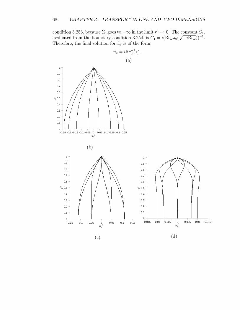
68 CHAPTER 3. TRANSPORT IN ONE AND TWO DIMENSIONS
condition 3.253, because Y0 goes to −∞ in the limit r∗ → 0. The constant C1,evaluated from the boundary condition 3.254, is C1 = ı(ReωJ0(
√−ıReω))−1.
Therefore, the final solution for uz is of the form,
uz = ıRe−1ω (1−
(a)
-0.25 -0.2 -0.15 -0.1 -0.05 0 0.05 0.1 0.15 0.2 0.25ux
∗
0
0.1
0.2
0.3
0.4
0.5
0.6
0.7
0.8
0.9
1
z∗
(b)
-0.15 -0.1 -0.05 0 0.05 0.1 0.15ux
∗
0
0.1
0.2
0.3
0.4
0.5
0.6
0.7
0.8
0.9
1
z∗
(c)
-0.015 -0.01 -0.005 0 0.005 0.01 0.015ux
∗
0
0.1
0.2
0.3
0.4
0.5
0.6
0.7
0.8
0.9
1
z∗
(d)

3.5. EFFECT OF PRESSURE ON MOMENTUM TRANSPORT 69
The velocity u∗z, equation 3.121, as a function of r∗, for Reω = 0.1 (a),
Reω = 1.0 (b), Reω = 10.0 (c) and Reω = 100.0 (d). The profiles, form rightto left, are at t∗ = 0, t∗ = (π/4), t∗ = (π/2), t∗ = (3π/4) and t∗ = π.
One way to obtain the solution in the limit of low Reynolds number, wecan use a Taylor series expansion of the solution 3.262 in the small parameterReω. Another method is to use an expansion of the equation 3.256 itself. Thelatter is useful even in more complicated situations where we are not ableto obtain an analytical solution for the velocity field, and it provides ourfirst encounter with the techniques of ‘regular’ and ‘singular’ perturbationexpansions. Therefore, we go through the analysis of the equation 3.256 inthe limits Reω ≪ 1 and Reω ≫ 1 in some detail.
In the limit Reω ≪ 1, we can obtain an approximate solution by consid-ering the limit Reω → 0 in equation 3.256. The solution uz in a series inReω,
uz = u(0)z + Reωu(1)
z + Re2ωu(2)
z + . . . (3.262)
This expansion is inserted into equation 3.256, to obtain,
ıReω(u(0)z + Reωu(1)
z + Re(2)ω ) =
1
r∗∂
∂r∗
(
r∗∂
∂r∗(u(0)
z + Reωu(1)z + Re2
ωu(2)z )
)
− 1
(3.263)We collect the coefficients of Re0
ω, Re1ω, Re2
ω, . . . in equation 3.263 to obtain,
1
r∗∂
∂r∗
(
r∗∂u(0)
z
∂r∗
)
− 1+
Reω
(
1
r∗∂
∂r∗
(
r∗∂u(1)
z
∂r∗
)
− ıu(0)z
)
+
Re2ω
(
1
r∗∂
∂r∗
(
r∗∂u(2)
z
∂r∗
)
− ıu(1)z
)
+
. . . = 0 (3.264)
In the limit Reω → 0, the first term on the left side of equation 3.264 isO(1) (independent of Reω), the second is O(Reω) (proportional to Reω), thethird term on the left is O(Re2
ω) (proportional to Re2ω), in the limit Reω → 0.
Here the symbol O(Reiω) (called ‘order of Reω power i’) indicates that that
term goes to zero as the ith power of the small parameter Reω in the limitReω → 0. If equation 3.264 is to be satisfied in the limit Reω → 0, thenthe individual coefficients of of Re0
ω, Re1ω, Re2
ω, . . . on the left side of equation

70 CHAPTER 3. TRANSPORT IN ONE AND TWO DIMENSIONS
3.264 should all be equal to zero. Therefore, we obtain a series of equations,
1
r∗∂
∂r∗
(
r∗∂u(0)
z
∂r∗
)
− 1 = 0 (3.265)
1
r∗∂
∂r∗
(
r∗∂u(1)
z
∂r∗
)
− ıu(0)z = 0 (3.266)
1
r∗∂
∂r∗
(
r∗∂u(2)
z
∂r∗
)
− ıu(1)z = 0 (3.267)
It is necessary to expand the boundary conditions also in a series in Reω.In the present example, this expansion is quite easy, because the bound-ary conditions 3.253 and 3.254 are homogeneous. Therefore, the boundaryconditions are of the form,
u(i)z = 0 at r∗ = 1 (3.268)
and∂u(i)
z
∂r∗= 0 at r∗ = 0 (3.269)
for i = 0, 1, 2, . . ..Equations 3.265, 3.266, and 3.267 can be solved sequentially to obtain
solutions for u(0)z , u(1)
z , u(2)z . The solutions are,
u(0)z = −(1 − r∗2)
4(3.270)
u(1)z =
ı(3 − 4r∗2 + r∗4)
64(3.271)
u(2)z =
(19 − 27r∗2 + 9r∗4 + r∗6)
2304(3.272)
Therefore, the final solution for u∗z in the limit Reω → 0, obtained by multi-
plying uz (equations 3.270, 3.271 and 3.272) by exp (ıt∗) and taking the realpart, is,
u∗z = −(1 − r∗2) cos (t∗)
4− Reω(3 − 4r∗2 + r∗4) sin (t∗)
64
+Re2
ω(19 − 27r∗2 + 9r∗4 + r∗6) cos (θ)
2304+ . . . (3.273)

3.5. EFFECT OF PRESSURE ON MOMENTUM TRANSPORT 71
Thus, this procedure, referred to as a ‘regular perturbation’ expansion, pro-vides a solution for the velocity field as a series in the small parameter Reω.
For zero Reynolds number, the velocity field is,
u∗z = −(1 − r∗2)
4cos (t∗) (3.274)
or the dimensional velocity field uz is,
uz = −K cos (ωt)R2
4µ
(
1 − r2
R2
)
(3.275)
This solution is identical to the steady solution 3.238, with the pressure gra-dient given by (K cos (ωt)), which is the instanteneous value of the pressuregradient at time t. The steady solution is recovered because the inertialterm on the left side of equation 3.233 has been neglected in the limit ofsmall Reynolds number. Physically, the Reynolds number Reω = (ωR2/ν)can be considered as the ratio of two time scales, the time period of oscilla-tion of the pressure field ω−1 and the time scale for momentum diffusion overa distance R, which is (R2/ν). When the Reynolds number is small, the timescale for momentum diffusion is small compared to the period of oscillationof the pressure field. Therefore, the velocity field responds instanteneouslyto the change in the pressure, and we obtain a solution that is identical tothe steady solution for the instanteneous value of the pressure gradient.
Next, we consider the limit Reω ≫ 1. In the high Reynolds number limit,it is necessary to scale the velocity by the inertial scale (ρω/K) in equation3.250, since we would expect a balance between the inertial forces and thepressure gradient when the viscous forces are small compared to the inertialforces. The non-dimensional velocity is defined as u∗∗
z = (ρuzω/K), and theequation 3.250 becomes,
∂u∗∗z
∂t∗=
1
Reω
1
r∗∂
∂r∗
(
r∗∂u∗∗
z
∂r∗
)
− cos (t∗) (3.276)
The substitutionu∗∗
z = Realu∗∗z exp (ıt∗)(3.277)
is used to obtain an ordinary differential equation for u∗∗,
ıu∗∗z =
1
Reω
1
r∗∂
∂r∗
(
r∗∂u∗∗
z
∂r∗
)
− 1 (3.278)
72 CHAPTER 3. TRANSPORT IN ONE AND TWO DIMENSIONS
A naive approximation in this limit would be to just neglect the viscousterm on the right in comparison to the inertial term on the left in equation3.278, to obtain,
ıu∗∗z = −1 (3.279)
This provides the solution for the velocity field as,
u∗∗z = ı (3.280)
This solution has to satisfy the boundary conditions 3.253 and 3.254. Bound-ary condition 3.254 is satisfied, but it is clear that we cannot satisfy boundarycondition 3.253, because we do not have any constants in the solution 3.280!Why?
The mathematical reason can be explained by examining the approxima-tion made in going from equation 3.278 to 3.279. Equation 3.278 is a secondorder differential equation in r∗, and so the solution of this equation willcontain two constants which are fixed by the boundary conditions. However,in going from equation 3.278 to 3.279, we neglected the highest derivative,because of the small factor Re−1
ω . In doing so, we have converted a differen-tial equation into an algebraic equation, and there are no constants in thesolution.
The physical reason for the inability to satisfy the no-slip condition atthe pipe wall is as follows. The velocity at the wall will decrease to zero onlyif the wall exerts a stress on the fliud, that is, if there is momentum diffusionfrom the wall to the fluid. In going from equation 3.278 to 3.279, we haveneglected the momentum diffusion, and so there is no shear stress exertedby the pipe wall on the fluid. Due to this, we are not able to satisfy theno-slip boundary condition. However, in the real pipe flow, there is a no-slipcondition at the surface which is satisfied by the actual flow. How can thisparadox be resolved?
We had neglected the momentum diffusion term in equation 3.279 becausethe Reynolds number Reω is small. The Reynolds number, Reω = (ωR2/ν),is the ratio of the time required for diffusion over a lenght scale R, ∼ (ν/R2),and the period of oscillation, ∼ ω−1. Even when this number is large, diffu-sion is still taking place, but the length scale to which momentum diffusesis smaller than R. Therefore, there is an ‘inner length scale’ at the wall ofthe pipe, which is the length scale over which diffusion takes place. Overa time period ∼ ω−1, this length scale is obviously (ν/ω)1/2 ∼ (RRe−1/2
ω ).Therefore, if we scale the distance from the wall by this inner length scale,
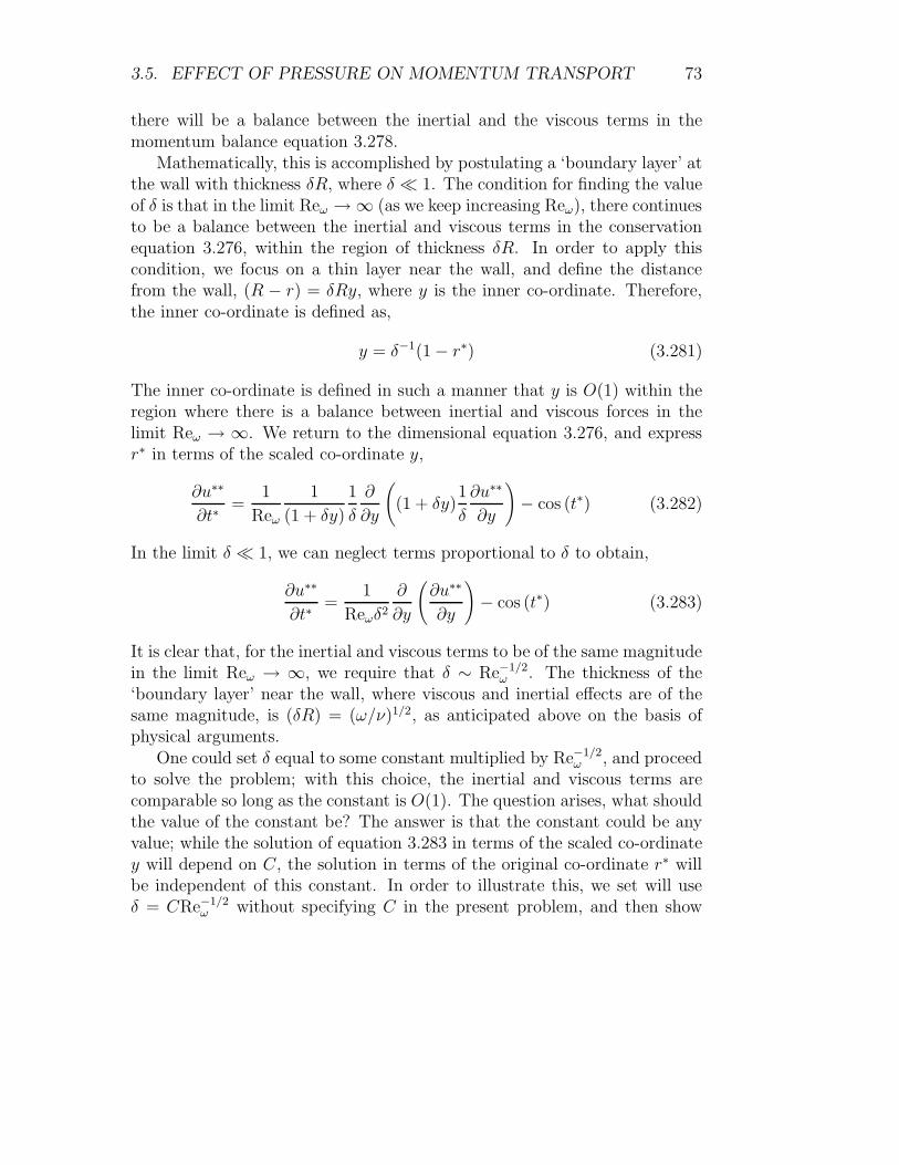
3.5. EFFECT OF PRESSURE ON MOMENTUM TRANSPORT 73
there will be a balance between the inertial and the viscous terms in themomentum balance equation 3.278.
Mathematically, this is accomplished by postulating a ‘boundary layer’ atthe wall with thickness δR, where δ ≪ 1. The condition for finding the valueof δ is that in the limit Reω → ∞ (as we keep increasing Reω), there continuesto be a balance between the inertial and viscous terms in the conservationequation 3.276, within the region of thickness δR. In order to apply thiscondition, we focus on a thin layer near the wall, and define the distancefrom the wall, (R − r) = δRy, where y is the inner co-ordinate. Therefore,the inner co-ordinate is defined as,
y = δ−1(1 − r∗) (3.281)
The inner co-ordinate is defined in such a manner that y is O(1) within theregion where there is a balance between inertial and viscous forces in thelimit Reω → ∞. We return to the dimensional equation 3.276, and expressr∗ in terms of the scaled co-ordinate y,
∂u∗∗
∂t∗=
1
Reω
1
(1 + δy)
1
δ
∂
∂y
(
(1 + δy)1
δ
∂u∗∗
∂y
)
− cos (t∗) (3.282)
In the limit δ ≪ 1, we can neglect terms proportional to δ to obtain,
∂u∗∗
∂t∗=
1
Reωδ2
∂
∂y
(
∂u∗∗
∂y
)
− cos (t∗) (3.283)
It is clear that, for the inertial and viscous terms to be of the same magnitudein the limit Reω → ∞, we require that δ ∼ Re−1/2
ω . The thickness of the‘boundary layer’ near the wall, where viscous and inertial effects are of thesame magnitude, is (δR) = (ω/ν)1/2, as anticipated above on the basis ofphysical arguments.
One could set δ equal to some constant multiplied by Re−1/2ω , and proceed
to solve the problem; with this choice, the inertial and viscous terms arecomparable so long as the constant is O(1). The question arises, what shouldthe value of the constant be? The answer is that the constant could be anyvalue; while the solution of equation 3.283 in terms of the scaled co-ordinatey will depend on C, the solution in terms of the original co-ordinate r∗ willbe independent of this constant. In order to illustrate this, we set will useδ = CRe−1/2
ω without specifying C in the present problem, and then show

74 CHAPTER 3. TRANSPORT IN ONE AND TWO DIMENSIONS
that the final solution does not depend on C. When we use this procedurein our later analysis of boundary layer theory, we will just use the simplestchoice C = 1.
Substituting δ = CRe−1/2ω in equation 3.283, we obtain,
∂u∗∗
∂t∗=
1
C
∂
∂y
(
∂u∗∗
∂y
)
− cos (t∗) (3.284)
As usual, we use the substitution u∗∗ = Real(u∗∗(y) exp (ıt∗)), to obtain anequation for u∗∗(y),
ı(y) =1
C
∂2
∂y2− 1 (3.285)
This is easily solved to obtain,
u∗∗ = ı + C1 exp (√
ıCy) + C2 exp−(√
ıCy) (3.286)
The constants in equation 3.286 are evaluated from the boundary condi-tions, which are to be re-expressed in terms of the scaled co-ordinate y. Theboundary condition 3.253, expressed in terms of y, is
u∗∗ = 0 at y = 0 (3.287)
The second boundary condition 3.254 is applied at r∗ = 0 which is equivalentto y = δ−1. In the limit δ → 0(Reω → ∞), this is equivalent to,
∂u∗∗
∂y= 0 for y → ∞ (3.288)
Using these two conditions, the constant C1 = 0 and C2 = −ı in equation3.286, and therefore, the final solution for u∗∗ is,
u∗∗ = ı(1 − exp (−√
ıCy)) (3.289)
Substituting y = (1− r∗)/δ and δ =√
CReω, the solution for u∗∗ in terms ofr∗ is,
u∗∗ = ı(1 − exp (−√
ıRe−1/2ω (1 − r∗)) (3.290)
As we had anticipated earlier, the solution for u∗∗ in terms of r∗ is indepen-dent of the constant C used in the definition of δ. Therefore, without lossof generality, we can set this constant to any value. In practice, it is mostconvenient to set this equal to 1.
The solution for u∗∗ is,
u∗∗ = Real(u∗∗)
= − sin (t∗)(1 − exp (−(1 − r∗)/√
2Reω) cos ((1 − r∗)/√
2Reω)) + cos (t∗) sin ((1 − r∗)/√
2Re(3.291)

3.6. SPHERICAL CO-ORDINATES: 75
3.6 Spherical co-ordinates:
The spherical co-ordinate system is used to analyse transport in or aroundobjects with spherical symmetry, such as spherical particles, bubbles or dropsimmersed in a fluid. If we were analysing the mass or energy transport froma spherical particle immersed in a fluid, it is preferable to have a co-ordinatesystem in which the surface of the particle is a surface on which one of theco-ordinates is a constant, so that boundary conditions can be easily appliedthere. The surface of a sphere in a Cartesian co-ordinate system is describedby the equation x2+y2+z2 = R2; clearly, this is not a convenient descriptionfor applying boundary conditions. In the spherical co-ordinate system, shownin figure ??, the three co-ordinates are the radius r, the distance from theorigin, the azimuthal angle θ, which is the angle made by the position vectorwith the z axis, and meridional angle φ, the angle made by the (projection ofthe position vector on the x− y plane) with the x axis. Surfaces of constantr are now spherical surfaces with radius r.
3.6.1 Balance equation:
Here, we consider one-dimensional transport, in which there is a variationof the concentration or temperature fields only in the radial direction. Inorder to obtain a balance equation, we consider a spherical shell bounded bytwo surfaces at r and r + ∆r. The volume of the shell is 4πr2∆r, while thesurface area is 4πr2. The terms in the mass balance equation, 3.1, for thisshell, are as follows. The accumulation of mass in the shell in a time ∆t is,
(
Accumulation of massin the shell
)
= (c(r, t + ∆t) − c(r, t))4πr2∆r (3.292)
The total mass entering the shell at r is the product of the mass flux, thesurface area, and the time interval ∆t,
(
Input ofmass into shell
)
= −(
jr(4πr2∆t))∣
∣
∣
r(3.293)
where jr is the mass flux in the radial direction. Similarly, the total massleaving the shell at r + ∆r is
(
Output ofmass from shell
)
=(
jr(4πr2∆t))∣
∣
∣
r+∆r(3.294)

76 CHAPTER 3. TRANSPORT IN ONE AND TWO DIMENSIONS
The source of mass in the differential volume is,(
Source ofmass in shell
)
= S(4πr2∆r∆t) (3.295)
where S is the amount of mass generated per unit volume per unit time.Substituting these into the balance condition ??, and dividing thoughout
by 4πr2δrδt, we obtain,
(c(r, t + ∆t) − c(r, t))
∆t=
1
r2∆r
(
(r2jr)∣
∣
∣
r− (r2jr)
∣
∣
∣
r+∆r
)
+ S (3.296)
Note that, as in the case of the cylindrical co-ordinate system, the surfacearea 4πr2 is a function of the radius r, and this surface area is different forthe surfaces at r and r + ∆r. Therefore, the factors r2 in the numerator anddenominator of the first two terms on the right side of equation 3.296 cannotbe cancelled. Taking the limit ∆r → 0 and ∆t → 0, the partial differentialequation for the concentration field is
∂c
∂t= − 1
r2
∂
∂r
(
r2jr
)
+ S (3.297)
The mass flux jr is related to the concentration gradient in the radial directionby the Fourier’s law for heat conduction,
jr = −D∂c
∂r(3.298)
With this, the mass balance equation becomes,
∂c
∂t=
1
r2
∂
∂r
(
r2D∂c
∂r
)
+ S (3.299)
When the diffusion coefficient is independent of position, the mass balanceequation reduces to,
∂c
∂t= D
1
r2
∂
∂r
(
r2 ∂c
∂r
)
+ S (3.300)
The energy balance equation for unidirectional transport in a sphericalco-ordinate system, derived in a similar manner, is,
∂T
∂t= α
1
r2
∂
∂r
(
r2∂T
∂r
)
+ Se (3.301)
where α = (k/ρCp) is the thermal diffusivity. The momentum balance equa-tion in a spherical co-ordinate system is more complicated, and so we deferdiscussion to a later chapter.

3.6. SPHERICAL CO-ORDINATES: 77
3.6.2 Steady diffusion from a sphere:
A spherical particle of radius R, with temperature T0 at the surface, is im-mersed in a fluid in which the temperature is T∞ far from the particle. Thesystem is at steady state, so that the temperature field does not vary withtime. We would like to find out the temperature variation in the fluid aroundthe particle, and the total amount of heat emitted by the particle per unittime.
The scaled radius and temperature are defined as, r∗ = (r/R) and T ∗ =(T − T∞)/(T0 − T∞). In terms of these scaled co-ordinates, the steady statebalance equation is,
1
r∗2
d
dr∗
(
r∗2 dT ∗
dr∗
)
= 0 (3.302)
with boundary conditions,
T ∗ = 0 for r∗ → ∞ (3.303)
T ∗ = 1 at r∗ = 1 (3.304)
Equation 3.302 is easily solved to obtain,
T ∗ =C1
r∗+ C2 (3.305)
where the constants, C1 and C2 are determined from the boundary conditions3.303 and 3.304. The final solution is,
T ∗ =1
r∗(3.306)
The dimensional temperature T is given by,
T = T∞ +(T0 − T∞)R
r(3.307)
The heat flux from the surface of the sphere is,
qr = −k∂T
∂r
= −k(T0 − T∞)
R
∂T ∗
∂r∗
=k(T0 − T∞)
Rr∗2(3.308)

78 CHAPTER 3. TRANSPORT IN ONE AND TWO DIMENSIONS
An important result is obtained if the temperature field is expressed interms of the total heat generated by the spherical surface, Q, instead of thetemperature at the surface. The total heat passing through any sphericalshell of radius r is the product of the heat flux and the radius of the shell,
Q = 4πr2qr
= 4πRk(T0 − T∞) (3.309)
From the energy balance condition, this is independent of the radius of theshell, since there is no generation or absorption of energy within the fluid.Using 3.309 to substitute for (T0 − T∞) in equation 3.307, we obtain,
T − T∞ =Q
4πKr(3.310)
When expressed in this manner, the temperature field does not depend onthe radius of the sphere R, but only on the total heat emitted by the sphereper unit time Q. Therefore, this solution is valid outside a sphere of anyradius, provided the total heat emitted per unit time is Q. Specifically, it isalso valid in the limit R → 0, the ‘point source’. The temperature field dueto a point source will be an important concept in our later discussion of theharmonic expansions.
3.6.3 Unsteady conduction in a sphere:
This problem is the analogue, in spherical co-ordinates, of the unsteady con-duction into a cylinder. A spherical particle of radius R and initial temper-ature T0 is immersed into a fluid with temperature T∞. The volume of thesurrounding fluid is considered to be large enough that the heat generatedfrom the particle does not increase the temperature of the fluid. We wouldlike to find out the variation of the temperature in the particle with time.
In the long time limit, we would expect the temperature of the particleto be equal to T∞. Therefore, we can define a scaled temperature T ∗ =(T − T∞)/(T0 − T∞), so that the scaled temperature is zero everywhere inthe long time limit. The scaled radius is defined as r∗ = (r/R), and thescaled time is t∗ = (tα/R2). With this, the unsteady energy balance equationbecomes,
∂T ∗
∂t∗=
1
r∗2
∂
∂r∗
(
r∗2 ∂T ∗
∂r∗
)
(3.311)

3.6. SPHERICAL CO-ORDINATES: 79
with the boundary condition at the surface of the sphere,
T ∗ = 0 at r∗ = 1 (3.312)
and initial condition that the temperature is equal to T0 everywhere withinthe sphere at t = 0,
T ∗ = 1 at
t∗ = 0 for r∗ < 1(3.313)Equation 3.311 is a second order differential equation in the radial co-
ordinate r∗, but we have specified only one boundary condition 3.312 at thesurface of the sphere. The second condition is the ‘symmetry’ condition atr∗ = 0, similar to the condition 3.205 at the axis of the cylindrical co-ordinatesystem. Since the temperature field is spherically symmetric, the derivativeof the temperature at the center will be independent of the direction ofapproach only if it is zero at the center,
∂T ∗
∂r∗= 0 at r∗ = 0 (3.314)
This is the symmetry condition at the origin of the spherical co-ordinatesystem.
Equation 3.311 is solved using the separation of variables procedure,where the temperature field is written as,
T ∗(r∗, t∗) = R(r∗)T (t∗) (3.315)
Using the separation of variables procedure (substitute the above expressionfor T ∗ into the conservation equation 3.311, and divide the equation by T ∗),we obtain equations for R and T ,
1
R1
r∗2
∂
∂r∗
(
r∗2∂R∂
)
= −β2 (3.316)
1
T∂T∂t∗
= −β2 (3.317)
where β is the eigenvalue to be determined from the boundary condition atthe surface of the sphere.
The equation 3.316 for R can be simplified as,
r∗2 ∂2R∂r∗2
+ 2r∗∂R∂r∗
+ β2r∗2R = 0 (3.318)
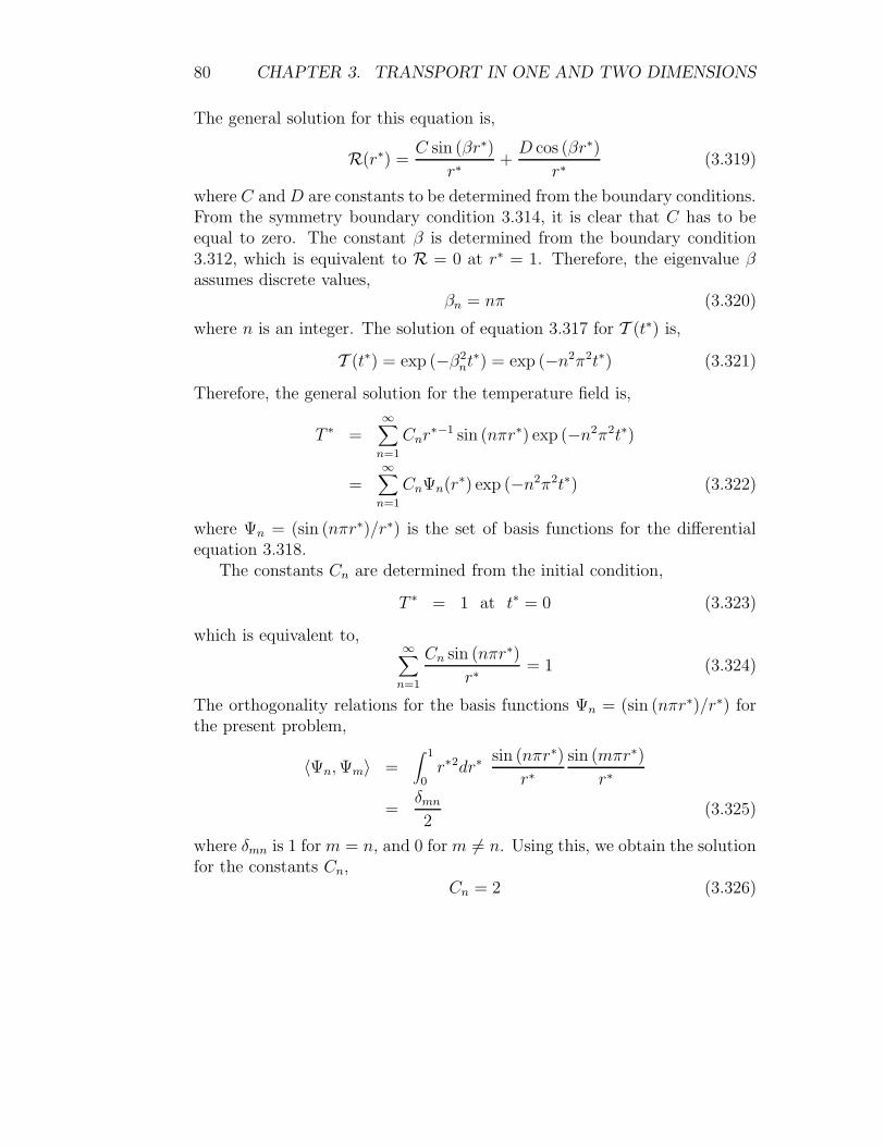
80 CHAPTER 3. TRANSPORT IN ONE AND TWO DIMENSIONS
The general solution for this equation is,
R(r∗) =C sin (βr∗)
r∗+
D cos (βr∗)
r∗(3.319)
where C and D are constants to be determined from the boundary conditions.From the symmetry boundary condition 3.314, it is clear that C has to beequal to zero. The constant β is determined from the boundary condition3.312, which is equivalent to R = 0 at r∗ = 1. Therefore, the eigenvalue βassumes discrete values,
βn = nπ (3.320)
where n is an integer. The solution of equation 3.317 for T (t∗) is,
T (t∗) = exp (−β2nt∗) = exp (−n2π2t∗) (3.321)
Therefore, the general solution for the temperature field is,
T ∗ =∞∑
n=1
Cnr∗−1 sin (nπr∗) exp (−n2π2t∗)
=∞∑
n=1
CnΨn(r∗) exp (−n2π2t∗) (3.322)
where Ψn = (sin (nπr∗)/r∗) is the set of basis functions for the differentialequation 3.318.
The constants Cn are determined from the initial condition,
T ∗ = 1 at t∗ = 0 (3.323)
which is equivalent to,∞∑
n=1
Cn sin (nπr∗)
r∗= 1 (3.324)
The orthogonality relations for the basis functions Ψn = (sin (nπr∗)/r∗) forthe present problem,
〈Ψn, Ψm〉 =∫ 1
0r∗2dr∗
sin (nπr∗)
r∗sin (mπr∗)
r∗
=δmn
2(3.325)
where δmn is 1 for m = n, and 0 for m 6= n. Using this, we obtain the solutionfor the constants Cn,
Cn = 2 (3.326)

3.6. SPHERICAL CO-ORDINATES: 81
3.6.4 Similarity solution for diffusion from a point source:
The scaled temperature is defined as T ∗ = ((T −T∞)/T∞), so that the scaledtemperature is zero in the limit r → ∞. The heat conduction equation inthe fluid is,
∂T ∗
∂t= α
(
1
r2
d
dr
(
r2dT ∗
dr
))
(3.327)
One of the boundary conditions are that T ∗ → 0 in the limit r → ∞,while the other is the flux condition at the source, which requires that thetotal amount of heat emitted per unit time is Q. Therefore, the flux from aspherical surface of radius r around the point source is (Q/(4πr2))
−KT∞dT ∗
dr=
Q
4πr2(3.328)
in the limit r → 0.As before, the equation ?? can be expressed in terms of a similarity
variable,d2T ∗
dξ2+
(
2
ξ+
ξ
2
)
dT ∗
dξ= 0 (3.329)
This equation can be solved to obtain the
dT ∗
dξ=
C
ξ2exp (−ξ2/4) (3.330)
The temperature can be obtained by integrating the above equation withrespect to ξ, and realising that T = 0 as ξ → ∞.
T ∗ =∫ ξ
∞dξ′
C
ξ′2 exp (−ξ′2/4)(3.331)
The above equation shows that the temperature at the surface of the wire isundefined, because the integral in equation ?? increases proportional to ξ−1
as ξ → ∞.The constant C can be determined from the flux condition, in the limit
r → 0(ξ → 0),
KdT ∗
dr= − Q
4πr2(3.332)
When expressed in terms of ξ, this is equivalent to
dT ∗
dξ= − Q
2πKξ(3.333)

82 CHAPTER 3. TRANSPORT IN ONE AND TWO DIMENSIONS
x
z
Figure 3.15: Flow of immiscible fluids.
Inserting solution ?? into the above equation, we find that the constantC = (Q/2πK). Therefore, the solution for the temperature field is,
T ∗ =Q
2πk
∫ ξ
∞dξ′
1
ξ′exp (−ξ′2/4) (3.334)
Adjacent flow of two immiscible liquids.
This is an example which illustrates the application of boundary conditionsbetween two immiscible liquids. Two immiscible liquids flow through a chan-nel of length L and width W under the influence of a pressure gradient, asshown in figure 3.15. The flow rates are adjusted such that the channel ishalf filled with fluid I (more dense phase) and half filled with fluid II (lessdense phase). It is necessary to find the distribution or velocity in this case.
The momentum balance is similar to that for the flow in a pressure gra-dient shown in the last example. The pressure balance reduces to
dτxz
dx+
p0 − pL
L= 0 (3.335)
This equation is valid in either phase I or phase II. Integration gives tworelations in the two phases.
τ (I)xz = −
(
p0 − pL
L
)
x + C(I)
τ (II)xz = −
(
p0 − pL
L
)
x + C(II) (3.336)

3.6. SPHERICAL CO-ORDINATES: 83
We can make use of one of the boundary conditions, that the stress is equalat the interface, to relate C(I) and C(II).
Atx = 0 τ (I)xz = τ (II)
xz
C(I) = C(II) (3.337)
Using Newton’s law of viscosity to relate the stress to the strain rate, we get
µ(I) dv(I)z
dx= −
(
p0 − pL
L
)
x + C(I)
µ(II)dv(II)z
dx= −
(
p0 − pL
L
)
x + C(II) (3.338)
This can be integrted to give
v(I)z = −
(
p0 − pL
2µ(I)L
)
x2 +C(I)x
µ(I)+ C
(I)2
v(II)z = −
(
p0 − pL
2µ(II)L
)
x2 +C(I)x
µ(I)+ C
(II)2
(3.339)
There are three constants in the above equations, which are determined usingthe three available boundary conditions.
Atx = 0 v(I)z = v(II)
z
Atx = −b v(I)z = 0
Atx = b v(II)z = 0 (3.340)
These boundary conditions provide three relationships between the constantsC(I), C
(I)2 and C
(II)2 .
C(I)2 = C
(II)2
0 = −(
p0 − pL
2µ(I)L
)
b2 − C(I)b
µ(I)+ C
(I)2
0 = −(
p0 − pL
2µ(II)L
)
b2 +C(I)b
µ(I)+ C
(I)2 (3.341)
These can be solved to obtain
C1 =(p0 − pL)b
2L
(
µ(I) − µ(II)
µ(I) + µ(II)
)
C(I)2 =
(p0 − pL)b2
2µ(I)L
(
2µ(I)
µ(I) + µ(II)
)
(3.342)

84 CHAPTER 3. TRANSPORT IN ONE AND TWO DIMENSIONS
Therefore, the velocity profiles in each layer are
v(I)z =
(p0 − pL)b2
2µ(I)L
[(
2µ(I)
µ(I) + µ(II)
)
+
(
µ(I) − µ(II)
µ(I) + µ(II)
)
x
b− x2
b2
]
v(I)z =
(p0 − pL)b2
2µ(II)L
[(
2µ(II)
µ(I) + µ(II)
)
+
(
µ(I) − µ(II)
µ(I) + µ(II)
)
x
b− x2
b2
]
(3.343)
Exercises
1. Consider a long and narrow channel two - dimensional of length L andheight H , where H ≪ L. The ends of the channel are closed so thatno fluid can enter or leave the channel. The bottom and side walls ofthe channel are stationary, while the top wall moves with a velocityV (t). Since the length of the channel is large compared to the height,the flow near the center can be considered as one dimensional. Nearthe ends, there will be some circulation due to the presence of the sidewalls, but this can be neglected far from the sides. For the flow farfrom the walls of the channel,
(a) Write the equations for the unidirectional flow. What are theboundary conditions? What restriction is placed on the velocityprofile due to the fact that the ends are closed and fluid cannotenter or leave the channel?
(b) If the wall is given a steady velocity V which is independent oftime, solve the equations (neglecting the time derivative term).Calculate the gradient of the pressure.
(c) If the wall is given an oscillating velocity V cos (ωt), obtain anordinary differential equation to obtain the velocity profile. Getan analytical solution for this which involves the constants of ite-gration. Use the boundary conditions to determine all unknownconstants.
2. In shell-and-tube heat exchangers, the tube side often has fins in orderto increase the conduction rate, as shown in figure 1. The fin canbe modeled, in two dimensions, as a rectangular block of length L,height H and with thermal conductivity k. One surface (outer wallof the tube of the heat exchanger) is at the temperature Tt, which isthe temperature of the tube side fluid. The other three surfaces are

3.6. SPHERICAL CO-ORDINATES: 85
at the temperature Ts, which is the temperature of the shell side fluid.Determine the heat flux from the fin as follows.
(a) Write down the conduction equation, ∇2T = 0, in two dimensions,and specify the boundary conditions.
(b) Define a non-dimensional temperature in such a way that bothboundary conditions are homogeneous along one of the co-ordinates.
(c) Use separation of variables to obtain separate the dependence ofT on the x and y co-ordinates.
(d) Write down the final solution for the temperature field which sat-isfies homogeneous boundary conditions.
(e) Determine the coefficients using orthogonality relations along theinhomogeneous direction. From this, calculate the heat flux as afunction of the temperature difference.
3. A rectangular channel of width W and height H is used for transportingfluid of density ρ and viscosity µ. If a steady pressure difference ∆p isapplied across the length L of the channel, determine the flow rate.
(a) First, obtain the momentum balance for the streamwise velocityfor a differential volume in the channel.
(b) Solve the equation using separation of variables to obtain the ve-locity. Note that the fluid velocity is zero on all the walls of thechannnel.
4. Consider a cylinder in a thin annular region, as shown in figure 3.16.The cylinder is pulled with a constant velocity V. The pressure is equalon both sides of the cylinder. Determine the fluid velocity, and the flowrate.
5. A fluid is contained in the annular region between two concentric cylin-ders of radius R1 and R2 moving with angular velocities Ω1 and Ω2.The gravitational field acts along the axis of the cylinders as shown infigure. The vessel is tall enough that the flow can be considered unidi-rectional when the distance from the bottom is large compared to thegap width (R1−R2). In this case, choose a coordinate system and writedown the mass and momentum conservation equations. Solve these for

86 CHAPTER 3. TRANSPORT IN ONE AND TWO DIMENSIONS
Outer radius R
Inner radius k R
V
Pressure pPressure p
Figure 3.16: Wire coating of dies.
the pressure and velocity fields. Can you find the equation for the freesurface?
6. Consider the unidirectional flow of a ‘power law fluid’ through a pipeof radius R, where the flow takes place only in the axial direction andthere is no radial flow. Use a polar coordinate system where the flowis in the x direction, and the radial vector is in the r direction. Theconstitutive relation for the shear stress τxr for this fluid is given by
τxr = kn
∣
∣
∣
∣
∣
dux
dr
∣
∣
∣
∣
∣
n−1 (dux
dr
)
(a) Use a momentum balance in the axial direction to determine equa-tion for the variation in the velocity as a function of the pressuregradient.
(b) What are the boundary conditions?
(c) Assume the pressure gradient is a constant, and solve the equationto obtain the velocity profile.
7. Consider the annular flow of two fluids in a tube, as shown in figure2, driven by a pressure difference applied across the ends of the tube.The tube radius is Ro, while the radius of the interface between thetwo fluids is Ri. The viscosities of the two fluids are µi and µo. Assumethat the densities of the two fluids are equal.

3.6. SPHERICAL CO-ORDINATES: 87
(a) Write down momentum balance equations for the two fluids. (Donot try to derive it, but use expressions already derived in thenotes).
(b) What are the boundary conditions, and the interface conditionsbetween the two fluids?
(c) How are the pressures and pressure gradients in the two fluidsrelated?
(d) Solve the momentum conservation equations to obtain the veloc-ity fields in the two fluids. From this, calculate the relationshipbetween friction factor and the Reynolds numbers based on theaverage velocity and viscosity of the two fluids.
8. A resistance heating appratus for a fluid consists of a thin wire im-mersed in a fluid. In order to design the appratus, it is necessary todetermine the temperature in the fluid as a function of he heat fluxfrom the wire. For the purposes of the calculation, the wire can beconsidered of infinite length so that the heat conduction problem iseffectively a two dimensional problem. In addition, the thickness ofthe wire is considered small compared to any other length scales in theproblem, so that the wire is a line source of heat. The wire and thefluid are initially at a temperature T0. At time t = 0, the current isswitched on so that the wire acts as a source of heat, and the heattransmitted per unit length of the wire is Q. The heat conduction inthe fluid is determined by the unsteady state heat conduction equation
∂tT = K∇2T (3.344)
and the heat flux (heat conducted per unit area) is
K∇T (3.345)
where K is the thermal conductivity of the fluid.
(a) Choose an appropriate coordinate system, and write down theunsteady heat conduction equation.
(b) What are the boundary conditions? Give special attention o theheat flux condition at the wire, and note that the wire is consideredto be of infinitesimal radius.
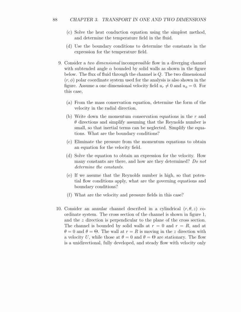
88 CHAPTER 3. TRANSPORT IN ONE AND TWO DIMENSIONS
(c) Solve the heat conduction equation using the simplest method,and determine the temperature field in the fluid.
(d) Use the boundary conditions to determine the constants in theexpression for the temperature field.
9. Consider a two dimensional incompressible flow in a diverging channelwith subtended angle α bounded by solid walls as shown in the figurebelow. The flux of fluid through the channel is Q. The two dimensional(r, φ) polar coordinate system used for the analysis is also shown in thefigure. Assume a one dimensional velocity field ur 6= 0 and uφ = 0. Forthis case,
(a) From the mass conservation equation, determine the form of thevelocity in the radial direction.
(b) Write down the momentum conservation equations in the r andθ directions and simplify assuming that the Reynolds number issmall, so that inertial terms can be neglected. Simplify the equa-tions. What are the boundary conditions?
(c) Eliminate the pressure from the momentum equations to obtainan equation for the velocity field.
(d) Solve the equation to obtain an expression for the velocity. Howmany constants are there, and how are they determined? Do not
determine the constants.
(e) If we assume that the Reynolds number is high, so that poten-tial flow conditions apply, what are the governing equations andboundary conditions?
(f) What are the velocity and pressure fields in this case?
10. Consider an annular channel described in a cylindrical (r, θ, z) co-ordinate system. The cross section of the channel is shown in figure 1,and the z direction is perpendicular to the plane of the cross section.The channel is bounded by solid walls at r = 0 and r = R, and atθ = 0 and θ = Θ. The wall at r = R is moving in the z direction witha velocity U , while those at θ = 0 and θ = Θ are stationary. The flowis a unidirectional, fully developed, and steady flow with velocity only

3.6. SPHERICAL CO-ORDINATES: 89
φ
r
αWall
Wall
in the z direction. The equation for the velocity field in the z directionis,
µ
(
1
r
∂
∂r
(
r∂uz
∂r
)
+1
r2
∂2uz
∂θ2
)
= 0
where µ is the viscosity.
(a) What are the boundary conditions required for solving the aboveequation?
(b) Use separation of variables, by writing uz = F (r)T (θ), and obtainequations for F and T .
(c) Find the solution for T (θ) that satisfies the boundary conditions.
(d) Find the solution for F (r), and enforce boundary conditions tofind the final solution.
11. A piston damper assembly, shown in figure 1, consists of a cylindricalpiston rod moving through a stationary cylindrical sleeve which is filledwith fluid. The sleeve is closed at both ends so that the fluid cannotmove in or out of the sleeve. The radius of the piston rod is Rp, whilethe outer radius of the sleeve is Rs. The length of the sleeve L is largecompared to the radius Rs. The piston rod moves with a velocity Uwith respect to the sleeve. Consider the region away from the endsof the sleeve, where the flow is expected to be in only one direction(parallel to the walls).

90 CHAPTER 3. TRANSPORT IN ONE AND TWO DIMENSIONS
Figure 3.17:
(a) Which is the non-zero component of the velocity in this co-ordinatesystem, and which spatial co-ordinate does the velocity dependon? Write the boundary conditions in the center region awayfrom the ends of the sleeve, where the flow is expected to be uni-directional.
(b) What condition can be obtained about the velocity in the centerof the channel (away from the ends) from mass conservation?
(c) Use a shell balance to derive the momentum conservation equationfor the unidirectional flow in the center of the sleeve away fromthe ends.
(d) Solve the momentum conservation equation to determine the ve-locity field.
12. Consider the fully developed flow in a circular tube with velocity profile
ux = U(t)
(
1 − r2
R2
)
as shown in figure 1, where the maximum velocity U could be a functionof t, but is independent of the stream-wise co-ordinate x. There is

3.6. SPHERICAL CO-ORDINATES: 91
Pis
ton
Flu
id
RR ps
Sleeve
Closed end
Closed end
L
Figure 3.18:
viscous dissipation which generates heat within the fluid, and the heatgenerated per unit volume of the fluid per unit time is given by,
Q = µ
(
∂ux
∂r
)2
Due to this, there is a temperature variation across the tube, and thetemperature field is governed by the convection-diffusion equation,
ρCv
(
∂T
∂t+ u.∇T
)
= k∇2T + Q
The temperature at the wall of the tube is maintained at T = T0,and we assume that the temperature could be a function oftime, but the temperature field is ‘fully developed’ so thatthe temperature is independent of the flow (x) direction.
(a) Choose a suitable co-ordinate system, and write down the convection-diffusion equation for the time-dependent but ‘fully developed’temperature field.
(b) Scale the co-ordinates and time. What would you use to scale thetemperature?

92 CHAPTER 3. TRANSPORT IN ONE AND TWO DIMENSIONS
(c) Obtain the solution for the temperature at steady state, whereboth the maximum velocity U and temperature are independentof time.
(d) If the maximum velocity has a sinusoidal variation, U(t) = U cos (ωt),what is the value of the heat source Q? How would you express theinhomogeneous term in the time-dependent convection-diffusionequation for the temperature in order to obtain a solution?
(e) Determine the solution for the temperature field.
Rx
r
0T=T
T=T0
13. An ideal vortex is a flow with circular streamlines where the particlemotion is incompressible and irrotational. The velocity profile obeysthe equation in cylindrical coordinates:
vθ =Γ
2πr(3.346)
with vr = vz = 0. At the origin, the above equation indicates that thevelocity becomes infinite. But this is prohibited because viscous forcesbecome important and the flow is rotational in a small region near thecore.
Consider an ideal vortex in which the velocity is given by the aboveequation for t < 0, and the core velocity is constrained to be zero att = 0. Find the velocity profile for t > 0. Assume that vθ is the onlynon - zero velocity component.

3.6. SPHERICAL CO-ORDINATES: 93
14. A cubic solid of side a is initially held at a temperature T0. At timest ≥ 0, its lateral faces are held at temperatures TA, TB, T0 and T0 as il-lustrated in figure 3.19. The top and bottom faces are insulated so thatno heat is transferred through them. The cube has heat conductivityC, density ρ and thermal conductivity K.
(a) Solve for the steady state temperature in the cube.
(b) Show how the transient problem may be set up in a form to whichseparation of variables can be applied.
q=0
q=0
T0 T0
T
T
A
B
Figure 3.19: Conduction from a cube.
15. A rotating cylinder geometry consists of a cylinder of radius R andheight H , filled with fluid, with two end caps. The cylinder rotates withan angular velocity Ω, while the end caps are stationary. Determinethe fluid velocity field using separation of variables as follows.
(a) Choose a coordinate system for the problem. Clearly, the onlynon-zero component of the velocity is uφ. Determine the boundaryconditions for this component of the velocity.

94 CHAPTER 3. TRANSPORT IN ONE AND TWO DIMENSIONS
(b) Write down the mass balance condition for an incompressible fluid.For a uni-directional flow in which the density is a constant, whatdoes this reduce to?
(c) Use a shell balance to determine the conservation equation for thevelocity. Can you eliminate the pressure term using a result fromthe mass balance condition?
(d) Solve the conservation equation at steady state using the methodof separation of variables. Frame the orthogonality conditionswhich would be required to solve the problem.
Data:
(a) Bessel equation:
x2 d2y
dx2+ x
dy
dx+ (x2 − n2)y = 0
Solution:y = A1Jn(x) + A2Yn(x)
where Jn(x) is bounded for x → 0, and Yn(x) is bounded forx → ∞. tem Modified Bessel equation:
x2 d2y
dx2+ x
dy
dx− (x2 + n2)y = 0
Solution:y = A1In(x) + A2Kn(x)
where In(x) is bounded for x → 0, and Kn(x) is bounded forx → ∞.