Chapter 3 Solving Ordinary Differential Equations in R

Chapter 3Solving Ordinary Differential Equations in R

Abstract Both Runge-Kutta and linear multistep methods are available to solveinitial value problems for ordinary differential equations in the R packages deSolveand deTestSet. Nearly all of these solvers use adaptive step size control, some alsocontrol the order of the formula adaptively, or switch between different types ofmethods, depending on the local properties of the equations to be solved. We showhow to trigger the various methods using a variety of applications pointing, wherenecessary, to problems that may arise. For instance, many practical applicationsinvolve discontinuities. As the integration routines assume that a solution issufficiently differentiable over a time step, handing such discontinuities requiresspecial consideration. We give examples of how we can implement a nonsmoothforcing term, switching behavior, and problems that include sudden jumps in thedependent variables. Since much computational efficiency can be gained by usingthe correct method for a particular problem, we end this chapter by providing a fewguidelines as to how the most efficient solution method for a particular problem canbe found.

3.1 Implementing Initial Value Problems in R

The R package deSolve [26] has several built-in functions for computing anumerical solution of initial value problems for ODEs.

They comprise methods to solve stiff and non-stiff problems, that deal with full,banded or arbitrarily sparse Jacobians etc. . . The methods included and the originalsource are listed in Sect. A.3.

A simplified form of the syntax for solving ODEs is:

ode(y, times, func, parms, ...)

where times holds the times at which output is wanted, y holds the initialconditions, func is the name of the R function that describes the differentialequations, and parms contains the parameter values (or is NULL). Many additionalinputs can be provided, e.g. the absolute and relative error tolerances (defaults

DOI 10.1007/978-3-642-28070-2 3, © Springer-Verlag Berlin Heidelberg 201241K. Soetaert et al., Solving Differential Equations in R, Use R!,

42 3 Solving Ordinary Differential Equations in R

rtol = 1e-6, atol = 1e-6), the maximal number of steps (maxsteps),the integration method etc. The default integration method is lsoda. If we type?lsoda a help page is opened that contains a list of all options that can be changed.As all these options have a default value, we are not obliged to assign a value tothem, as long as we are content with the default.

3.1.1 A Differential Equation Comprising One Variable

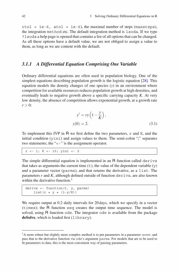
Ordinary differential equations are often used in population biology. One of thesimplest equations describing population growth is the logistic equation [28]. Thisequation models the density changes of one species (y) in an environment wherecompetition for available resources reduces population growth at high densities, andeventually leads to negative growth above a specific carrying capacity K. At verylow density, the absence of competition allows exponential growth, at a growth rater > 0:

y′ = ry(

1− yK

),

y(0) = 2. (3.1)

To implement this IVP in R we first define the two parameters, r and K, and theinitial condition (yini) and assign values to them. The semi-colon “;” separatestwo statements; the “<-” is the assignment operator.

r <- 1; K <- 10; yini <- 2

The simple differential equation is implemented in an R function called derivsthat takes as arguments the current time (t), the value of the dependent variable (y)and a parameter vector (parms), and that returns the derivative, as a list. Theparameters r and K, although defined outside of function derivs, are also knownwithin the derivative function.1

derivs <- function(t, y, parms)list(r * y * (1-y/K))

We require output at 0.2 daily intervals for 20 days, which we specify in a vector(times); the R function seq creates the output time sequence. The model issolved, using R function ode. The integrator ode is available from the packagedeSolve, which is loaded first (library).

1A more robust but slightly more complex method is to put parameters in a parameter vector, andpass that to the derivative function via ode’s argument parms. For models that are to be used tofit parameters to data, this is the most convenient way of passing parameters.

3.1 Implementing Initial Value Problems in R 43

0 5 10 15 20

2

4

6

8

10

12

logistic growth

time

Fig. 3.1 A simple initialvalue problem, solved twicewith different initialconditions. See text for the Rcode

library(deSolve)times <- seq(from = 0, to = 20, by = 0.2)out <- ode(y = yini, times = times, func = derivs,

parms = NULL)

The model output in out is a matrix consisting of two columns, first time, thenthe state variable value y. We print the first three lines of this matrix:

head(out, n = 3)

time 1[1,] 0.0 2.000000[2,] 0.2 2.339222[3,] 0.4 2.716436

We now solve the differential equation with a different initial condition, y(0) = 12,and store the output in matrix out2:

yini <- 12out2 <- ode(y = yini, times = times, func = derivs,

parms = NULL)

The output of these two solutions is easily plotted, using the deSolve’s functionplot with the solid lines twice as thick as the default (lwd=2) (Fig. 3.1). It showsfor the first solution an initial fast increase of the density, levelling off towards thecarrying capacity K. The second solution shows a gradual decrease towards K.

plot(out, out2, main = "logistic growth", lwd = 2)


3.1.2 Multiple Variables: The Lorenz Model

It is only slightly more complex to write a model that describes the dynamics ofmultiple variables.

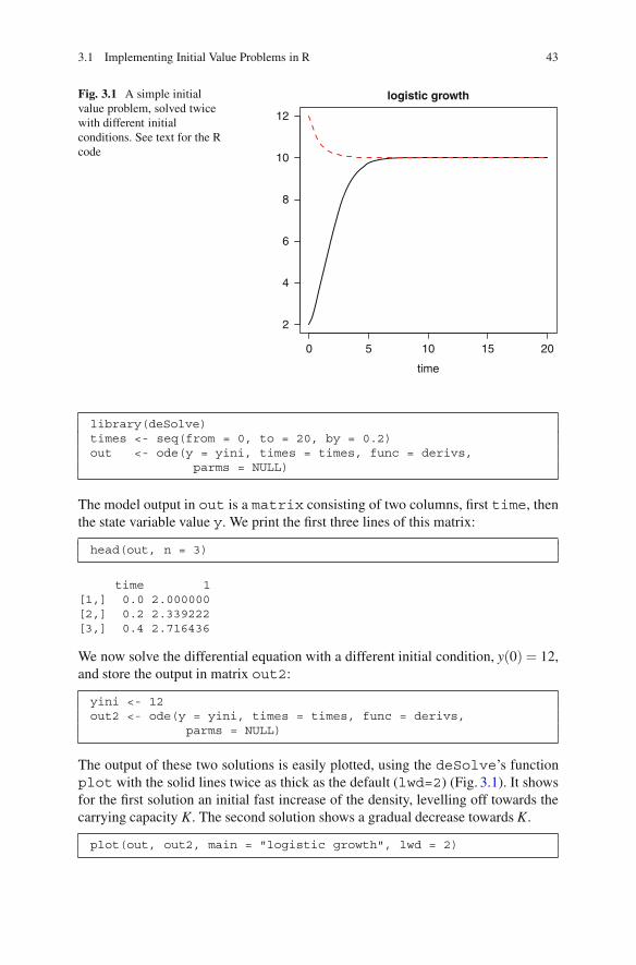
The Lorenz equations [18] were the first chaotic dynamical system of ordinarydifferential equations to be described. They consist of three ordinary differentialequations, expressing the dynamics of the variables, X , Y and Z that were assumedto represent idealized behavior of the Earth’s atmosphere. The model equations are:

X ′ = aX +YZ,

Y ′ = b(Y −Z),

Z′ = −XY + cY −Z, (3.2)

where X , Y and Z refer to the horizontal and vertical temperature distributionand convective flow, and a,b,c are parameters with values −8/3, −10 and 28respectively.

The R implementation starts by defining the parameter values and the initialcondition. For the latter, we create a three-valued vector using the function “c()”,naming the elements “X”, “Y” and “Z”. These names are handy, as we can use themin the derivative function so making the code more readable, but they also serve tolabel the output (see below).

a <- -8/3; b <- -10; c <- 28yini <- c(X = 1, Y = 1, Z = 1)

Within the derivative function (called Lorenz), we make the names of thevariables available by the construct with (as.list(y), {...}) . Note thatthis statement effectively embraces all other statements within the function (i.e. theclosing brackets “})” are the last before the curly braces terminating the function).

Similarly as in the previous example, the derivative function returns the deriva-tives, packed as a list, but now they are concatenated (c()) in a vector. Here it isextremely important 2 to return the values of the three derivatives, in the same orderas in which the initial conditions are defined. With yini containing the values ofvariablesX, Y and Z, the derivative vector should be returned as dX, dY, dZ.

Lorenz <- function (t, y, parms) {with(as.list(y), {

dX <- a * X + Y * ZdY <- b * (Y - Z)dZ <- -X * Y + c * Y - Zlist(c(dX, dY, dZ)) })

}

2it is the most common mistake that beginners make.

3.2 Runge-Kutta Methods 45

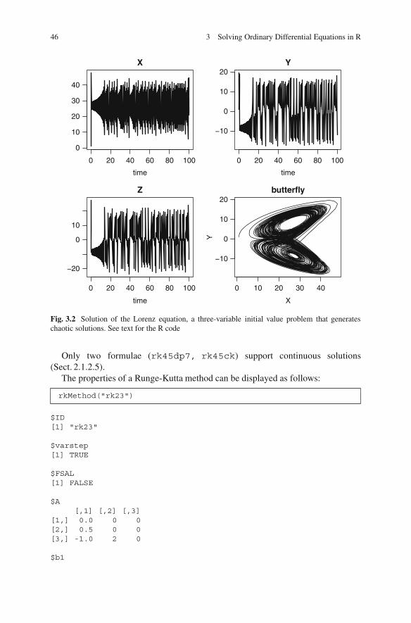
We solve the IVP for 100 days, producing output every 0.01 days; this small outputstep is necessary to obtain smooth figures. In general this does not affect the timestep of integration; this is usually determined by the solver.

times <- seq(from = 0, to = 100, by = 0.01)out <- ode(y = yini, times = times, func = Lorenz,

parms = NULL)

The output generated by the solvers from deSolve can conveniently be plottedusing deSolve’s method plot. This works slightly differently from R’s defaultplot method, as it depicts all variables at the same time, neatly arranged in severalrows and columns. Using this plot method saves a lot of R statements, especiallyif the model contains many variables.

The first statement in the code section below plots the three dependent variablesX, Y, Z in two rows and two columns. As we gave names to the initial conditions,the figures are correctly labeled (Fig. 3.2).

It is very simple to overrule this deSolve-specific plot function. By selectingspecific variables from out (here “X” and “Y”) rather than the entire output matrix,the default plotting method from R will be used. So, in the last statement, we depictvariable Y versus X to generate the famous “butterfly” (Fig. 3.2).

plot(out, lwd = 2)plot(out[,"X"], out[,"Y"], type = "l", xlab = "X",

ylab = "Y", main = "butterfly")

3.2 Runge-Kutta Methods

The R package deSolve contains a large number of Runge-Kutta methods(Sect. 2.1). With the following statement all implemented methods are shown:

rkMethod()

[1] "euler" "rk2" "rk4" "rk23" "rk23bs"[6] "rk34f" "rk45f" "rk45ck" "rk45e" "rk45dp6"[11] "rk45dp7" "rk78dp" "rk78f" "irk3r" "irk5r"[16] "irk4hh" "irk6kb" "irk4l" "irk6l" "ode23"[21] "ode45"

They comprise simple Runge-Kutta formulae (Heun’s method rk2, the classicalfourth order Runge-Kutta, rk4) and several explicit Runge-Kutta pairs of orders3(2) to orders 8(7). The embedded, explicit methods are according to Fehlberg [10](rk..f), Dormand and Prince [8, 9] (rk..dp.), Bogacki and Shampine [3](rk23bs, ode..) and Cash and Karp [7] (rk45ck).

The implicit Runge-Kutta’s (irk..) from this list are not optimally coded; abetter implicit Runge-Kutta is the (radau) method [11] that will be discussed inChaps. 4 and 5.


0 20 40 60 80 100

0

10

20

30

40

X

time

0 20 40 60 80 100

−10

0

10

20Y

time

0 20 40 60 80 100

−20

0

10

Z

time

0 10 20 30 40

−10

0

10

20butterfly

X

Y

Fig. 3.2 Solution of the Lorenz equation, a three-variable initial value problem that generateschaotic solutions. See text for the R code

Only two formulae (rk45dp7, rk45ck) support continuous solutions(Sect. 2.1.2.5).

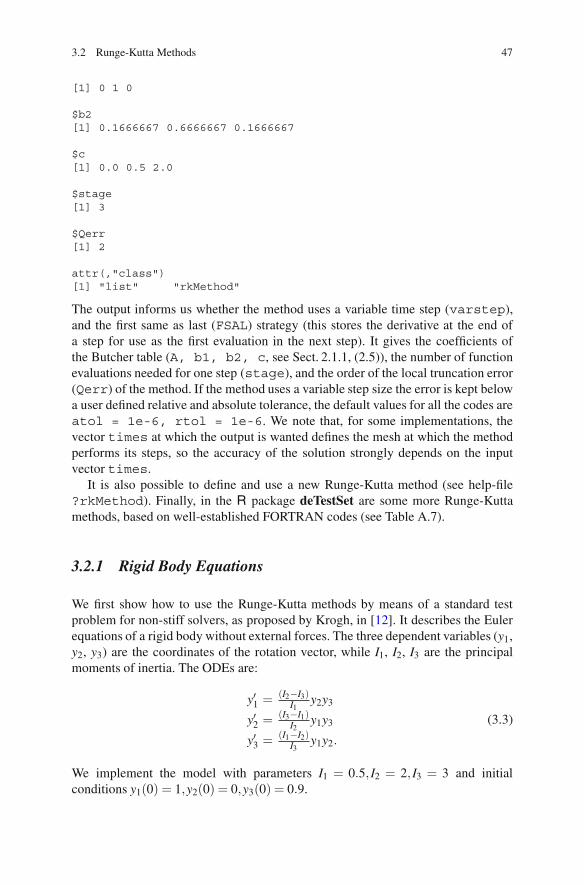
The properties of a Runge-Kutta method can be displayed as follows:

rkMethod("rk23")

$ID[1] "rk23"

$varstep[1] TRUE

$FSAL[1] FALSE

$A[,1] [,2] [,3]

[1,] 0.0 0 0[2,] 0.5 0 0[3,] -1.0 2 0

$b1


[1] 0 1 0

$b2[1] 0.1666667 0.6666667 0.1666667

$c[1] 0.0 0.5 2.0

$stage[1] 3

$Qerr[1] 2

attr(,"class")[1] "list" "rkMethod"

The output informs us whether the method uses a variable time step (varstep),and the first same as last (FSAL) strategy (this stores the derivative at the end ofa step for use as the first evaluation in the next step). It gives the coefficients ofthe Butcher table (A, b1, b2, c, see Sect. 2.1.1, (2.5)), the number of functionevaluations needed for one step (stage), and the order of the local truncation error(Qerr) of the method. If the method uses a variable step size the error is kept belowa user defined relative and absolute tolerance, the default values for all the codes areatol = 1e-6, rtol = 1e-6. We note that, for some implementations, thevector times at which the output is wanted defines the mesh at which the methodperforms its steps, so the accuracy of the solution strongly depends on the inputvector times.

It is also possible to define and use a new Runge-Kutta method (see help-file?rkMethod). Finally, in the R package deTestSet are some more Runge-Kuttamethods, based on well-established FORTRAN codes (see Table A.7).

3.2.1 Rigid Body Equations

We first show how to use the Runge-Kutta methods by means of a standard testproblem for non-stiff solvers, as proposed by Krogh, in [12]. It describes the Eulerequations of a rigid body without external forces. The three dependent variables (y1,y2, y3) are the coordinates of the rotation vector, while I1, I2, I3 are the principalmoments of inertia. The ODEs are:

y′1 = (I2−I3)I1

y2y3

y′2 = (I3−I1)I2

y1y3

y′3 = (I1−I2)I3

y1y2.

(3.3)

We implement the model with parameters I1 = 0.5, I2 = 2, I3 = 3 and initialconditions y1(0) = 1,y2(0) = 0,y3(0) = 0.9.


After loading the package deSolve and defining the initial conditions (yini),the model function is defined (rigidode). Although in previous examples, wemade the code more readable by using the names of the variables, here we use theirposition in the variable vector y, instead. Also, the parameter values are hard-coded.

library(deSolve)yini <- c(1, 0, 0.9)

rigidode <- function(t, y, parms) {dy1 <- -2 * y[2] * y[3]dy2 <- 1.25* y[1] * y[3]dy3 <- -0.5* y[1] * y[2]list(c(dy1, dy2, dy3))

}

The times at which output is wanted consists of a sequence of values, extendingover 20 days, and at 0.01 day intervals. The ODEs are solved with the Cash-KarpRunge-Kutta method (”rk45ck”), and the first three rows of this matrix are visuallyinspected (head).

times <- seq(from = 0, to = 20, by = 0.01)out <- ode (times = times, y = yini, func = rigidode,

parms = NULL, method = rkMethod("rk45ck"))head (out, n = 3)

time 1 2 3[1,] 0.00 1.0000000 0.00000000 0.9000000[2,] 0.01 0.9998988 0.01124950 0.8999719[3,] 0.02 0.9995951 0.02249603 0.8998875

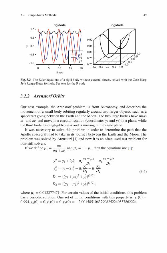
We could plot the three state variables, using deSolve’s plot method as in theprevious example. However, it is more instructive to plot all variables in one figureinstead (Fig. 3.3). We use R function matplot to do so. Rather than using thedefault settings of the function (points), we choose solid lines (type = "l",lty = "solid"), twice as thick as the default (lwd = 2) and with differentcolour for each state variable. The first column of out holds the time and is usedas the x-variable, while all except the first column (out[,-1]) are used as y-variables.

matplot(x = out[,1], y = out[,-1], type = "l", lwd = 2,lty = "solid", col = c("red", "blue", "black"),xlab = "time", ylab = "y", main = "rigidode")

legend("bottomright", col = c("red", "blue", "black"),legend = c("y1", "y2", "y3"), lwd = 2)

Another way of depicting the output is to plot the three coordinates of the rotationvector in a 3D plot. This can easily be done using the R package scatterplot3d [17].

library(scatterplot3d)scatterplot3d(out[,-1], type = "l", lwd = 2, xlab = "",

ylab = "", zlab = "", main = "rigidode")


0 5 10 15 20

−1.0

−0.5

0.0

0.5

1.0

rigidode

times

y

y1y2y3

rigidode

−1.0 −0.5 0.0 0.5 1.00.70

0.75

0.80

0.85

0.90

−1.0−0.5

0.00.5

1.0

Fig. 3.3 The Euler equations of a rigid body without external forces, solved with the Cash-Karp5(4) Runge-Kutta formula. See text for the R code

3.2.2 Arenstorf Orbits

Our next example, the Arenstorf problem, is from Astronomy, and describes themovement of a small body orbiting regularly around two larger objects, such as aspacecraft going between the Earth and the Moon. The two large bodies have massm1 and m2 and move in a circular rotation (coordinates y1 and y2) in a plane, whilethe third body has negligible mass and is moving in the same plane.

It was necessary to solve this problem in order to determine the path that theApollo spacecraft had to take in its journey between the Earth and the Moon. Theproblem was solved by Arenstorf [1] and now it is an often used test problem fornon-stiff solvers.

If we define μ1 =m1

m1 +m2and μ2 = 1− μ1, then the equations are [1]:

y′′1 = y1 + 2y′2 − μ2y1 + μ1

D1− μ1

y1 − μ2

D2

y′′2 = y2 − 2y′1 − μ2y2

D1− μ1

y2

D2

D1 = ((y1 + μ1)2 + y2

2)(3/2)

D2 = ((y1 − μ2)2 + y2

2)(3/2),

(3.4)

where μ1 = 0.012277471. For certain values of the initial conditions, this problemhas a periodic solution. One set of initial conditions with this property is: y1(0) =0.994,y2(0) = 0,y′1(0) = 0,y′2(0) =−2.00158510637908252240537862224.


Before solving these equations, we expand the second order equations in two firstorder ones (y3 = y′1 and y4 = y′2)

library(deSolve)Arenstorf <- function(t, y, p) {

D1 <- ((y[1] + mu1)ˆ2 + y[2]ˆ2)ˆ(3/2)D2 <- ((y[1] - mu2)ˆ2 + y[2]ˆ2)ˆ(3/2)dy1 <- y[3]dy2 <- y[4]dy3 <- y[1] + 2*y[4] - mu2*(y[1]+mu1)/D1 - mu1*(y[1]-mu2)/D2dy4 <- y[2] - 2*y[3] - mu2*y[2]/D1 - mu1*y[2]/D2return(list( c(dy1, dy2, dy3, dy4) ))

}mu1 <- 0.012277471mu2 <- 1 - mu1yini <- c(y1 = 0.994, y2 = 0,

dy1 = 0, dy2 = -2.00158510637908252240537862224)times <- seq(from = 0, to = 18, by = 0.01)

We solve the above IVP with the fifth order Dormand and Prince method(DOPRI5(4) [8]):

out <- ode(func = Arenstorf, y = yini, times = times,parms = 0, method = "ode45")

We can also solve the same problem with a second and third set of initial conditions:

yini2 <- c(y1 = 0.994, y2 = 0,dy1 = 0, dy2 = -2.0317326295573368357302057924)

out2 <- ode(func = Arenstorf, y = yini2, times = times,parms = 0, method = "ode45")

yini3 <- c(y1 = 1.2, y2 = 0,dy1 = 0, dy2 = -1.049357510)

out3 <- ode(func = Arenstorf, y = yini3, times = times,parms = 0, method = "ode45")

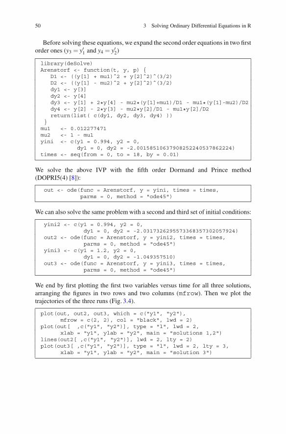
We end by first plotting the first two variables versus time for all three solutions,arranging the figures in two rows and two columns (mfrow). Then we plot thetrajectories of the three runs (Fig. 3.4).

plot(out, out2, out3, which = c("y1", "y2"),mfrow = c(2, 2), col = "black", lwd = 2)

plot(out[ ,c("y1", "y2")], type = "l", lwd = 2,xlab = "y1", ylab = "y2", main = "solutions 1,2")

lines(out2[ ,c("y1", "y2")], lwd = 2, lty = 2)plot(out3[ ,c("y1", "y2")], type = "l", lwd = 2, lty = 3,

xlab = "y1", ylab = "y2", main = "solution 3")

3.3 Linear Multistep Methods 51

0 5 10 15

−1.0

0.0

1.0

y1

time0 5 10 15

−1.0

0.0

1.0

y2

time

−1.0 −0.5 0.0 0.5 1.0

−1.0

0.0

1.0

solutions 1,2

y1

y2

−1.0 0.0 0.5 1.0

−0.6

−0.2

0.2

0.6

solution 3

y1

y2

Fig. 3.4 The Arenstorf problem, solved with the dopri5 Runge-Kutta method. See text for the Rcode

3.3 Linear Multistep Methods

The solvers vode [4], lsode [13], and lsodes [14] from the R packagedeSolve implement both variable-coefficient Adams methods as well as backwarddifferentiation formulas (the default) of variable order. The Adams methods arebetter suited for non-stiff problems, the BDF for stiff problems. In these codes, themaximal order for the Adams and BDF methods are 12 and 5 respectively. Whereasin the above-mentioned solvers, it is left to the user to specify whether to use a stiffor non-stiff method, the solver lsoda [19] will detect whether stiffness is presentor not, and trigger an appropriate change in the solution method if this property ofstiffness changes (see Sect. 2.7.3). This is such a robust procedure that lsoda is thedefault integration method chosen by ode.

In some cases, one may find it more efficient to select another integration methodrather than this default. Two implementations of the Adams methods are available,one that uses a predictor corrector implementation with a functional iteration asthe corrector (called “adams”), and a second that implements the implicit Adamsmethod (“impAdams”) by solving the implicit equation using chord iteration based


on the Jacobian (see Sect. 2.6). It is simplest to use the function ode with theappropriate method, to trigger a specific multistep method. For instance,

ode(y, times, func, parms, ...)ode(y, times, func, parms, method = "bdf", ...)ode(y, times, func, parms, method = "adams", ...)ode(y, times, func, parms, method = "impAdams", ...)ode(y, times, func, parms, method = vode, ...)

will use lsoda (the default method), the backward differentiation formula, andthe simple Adams and implicit Adams method (based on the code lsode), and themethod vode respectively. Note that it is allowed to pass both the name of thefunction, or the function itself.

Finally, more multistep methods are available from the package deTestSet: func-tions gamd [16] (implementing the generalized Adams methods), mebdfi [6] (themodified extended backward differentiation formula) and bimd[5] (implementingblock implicit methods). The calling sequence is:

library(deTestSet)ode(y, times, func, parms, method = gamd, ...)ode(y, times, func, parms, method = mebdfi, ...)ode(y, times, func, parms, method = bimd, ...)

or:

gamd(y, times, func, parms, ...)mebdfi(y, times, func, parms,...)bimd(y, times, func, parms,...)

These codes will be extensively used when we deal with solving DAEs, inChap. 5.

3.3.1 Seven Moving Stars

The Pleiades problem [12] is a celestial mechanics problem of seven stars, withmasses mi, in the two-dimensional plane of coordinates (x,y). The stars areconsidered to be point masses.

The only force acting on them is gravitational attraction, with gravitationalconstant G (units of m3kg−1s−2).

If ri j = (xi − x j)2 +(yi − y j)

2 is the square of the distance between stars i and j,then the second order equations describing their movement are given by:

x′′i = G ∑j �=i

m j(x j − xi)

r3/2i j

y′′i = G ∑j �=i

m j(y j − yi)

r3/2i j

,(3.5)


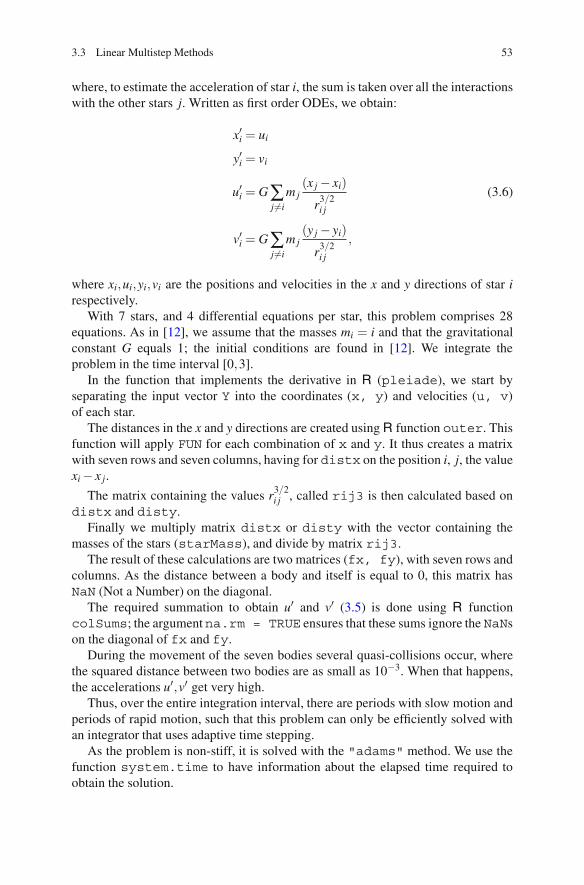
where, to estimate the acceleration of star i, the sum is taken over all the interactionswith the other stars j. Written as first order ODEs, we obtain:

x′i = ui

y′i = vi

u′i = G ∑j �=i

m j(x j − xi)

r3/2i j

(3.6)

v′i = G ∑j �=i

m j(y j − yi)

r3/2i j

,

where xi,ui,yi,vi are the positions and velocities in the x and y directions of star irespectively.

With 7 stars, and 4 differential equations per star, this problem comprises 28equations. As in [12], we assume that the masses mi = i and that the gravitationalconstant G equals 1; the initial conditions are found in [12]. We integrate theproblem in the time interval [0,3].

In the function that implements the derivative in R (pleiade), we start byseparating the input vector Y into the coordinates (x, y) and velocities (u, v)of each star.

The distances in the x and y directions are created using R function outer. Thisfunction will apply FUN for each combination of x and y. It thus creates a matrixwith seven rows and seven columns, having for distx on the position i, j, the valuexi − x j.

The matrix containing the values r3/2i j , called rij3 is then calculated based on

distx and disty.Finally we multiply matrix distx or disty with the vector containing the

masses of the stars (starMass), and divide by matrix rij3.The result of these calculations are two matrices (fx, fy), with seven rows and

columns. As the distance between a body and itself is equal to 0, this matrix hasNaN (Not a Number) on the diagonal.

The required summation to obtain u′ and v′ (3.5) is done using R functioncolSums; the argumentna.rm = TRUE ensures that these sums ignore the NaNson the diagonal of fx and fy.

During the movement of the seven bodies several quasi-collisions occur, wherethe squared distance between two bodies are as small as 10−3. When that happens,the accelerations u′,v′ get very high.

Thus, over the entire integration interval, there are periods with slow motion andperiods of rapid motion, such that this problem can only be efficiently solved withan integrator that uses adaptive time stepping.

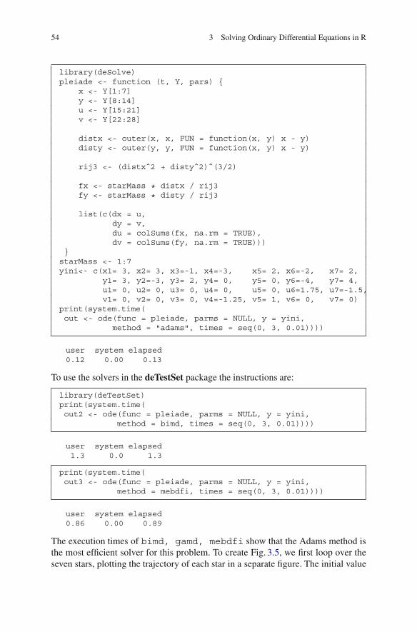
As the problem is non-stiff, it is solved with the "adams" method. We use thefunction system.time to have information about the elapsed time required toobtain the solution.


library(deSolve)pleiade <- function (t, Y, pars) {

x <- Y[1:7]y <- Y[8:14]u <- Y[15:21]v <- Y[22:28]

distx <- outer(x, x, FUN = function(x, y) x - y)disty <- outer(y, y, FUN = function(x, y) x - y)

rij3 <- (distxˆ2 + distyˆ2)ˆ(3/2)

fx <- starMass * distx / rij3fy <- starMass * disty / rij3

list(c(dx = u,dy = v,du = colSums(fx, na.rm = TRUE),dv = colSums(fy, na.rm = TRUE)))

}starMass <- 1:7yini<- c(x1= 3, x2= 3, x3=-1, x4=-3, x5= 2, x6=-2, x7= 2,

y1= 3, y2=-3, y3= 2, y4= 0, y5= 0, y6=-4, y7= 4,u1= 0, u2= 0, u3= 0, u4= 0, u5= 0, u6=1.75, u7=-1.5,v1= 0, v2= 0, v3= 0, v4=-1.25, v5= 1, v6= 0, v7= 0)

print(system.time(out <- ode(func = pleiade, parms = NULL, y = yini,

method = "adams", times = seq(0, 3, 0.01))))

user system elapsed0.12 0.00 0.13

To use the solvers in the deTestSet package the instructions are:

library(deTestSet)print(system.time(out2 <- ode(func = pleiade, parms = NULL, y = yini,

method = bimd, times = seq(0, 3, 0.01))))


print(system.time(out3 <- ode(func = pleiade, parms = NULL, y = yini,

method = mebdfi, times = seq(0, 3, 0.01))))


The execution times of bimd, gamd, mebdfi show that the Adams method isthe most efficient solver for this problem. To create Fig. 3.5, we first loop over theseven stars, plotting the trajectory of each star in a separate figure. The initial value


0 1 2 3

−4

−2

0

2

star 1

x

y

1.5 2.0 2.5 3.0

−3.2

−2.8

−2.4

star 2

x

y

−3 −2 −1 0

2.0

3.0

4.0

5.0

star 3

x

y

−3 −2 −1 0

−2.5

−1.5

−0.5

star 4

x

y

0.0 0.5 1.0 1.5 2.0

0.0

1.0

2.0

star 5

x

y

−2 −1 0 1

−4

−3

−2

−1

star 6

x

y

−0.5 0.5 1.5

1.0

2.0

3.0

4.0

star 7

x

y

−3 −1 1 2 3

−4

0

2

4

ALL

x

y

1

2

3

4 5

6

7

0.0 1.0 2.0 3.0

−20

−10

0

stars 1, 7

time

velo

city

u1u7

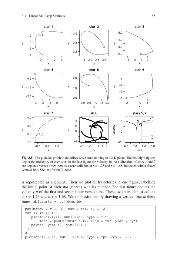
Fig. 3.5 The pleiades problem describes seven stars moving in a 2-D plane. The first eight figuresdepict the trajectory of each star; in the last figure the velocity in the x-direction of stars 1 and 7are depicted versus time; there is a near-collision at t = 1.23 and t = 1.68, indicated with a dottedvertical line. See text for the R code

is represented as a point. Then we plot all trajectories in one figure, labellingthe initial point of each star (text) with its number. The last figure depicts thevelocity u of the first and seventh star versus time. These two stars almost collideat t = 1.23 and at t = 1.68. We emphasise this by drawing a vertical line at thesetimes; abline(v =...) does this.

par(mfrow = c(3, 3), mar = c(4, 4, 3, 2))for (i in 1:7) {

plot(out[,i+1], out[,i+8], type = "l",main = paste("star ",i), xlab = "x", ylab = "y")

points (yini[i], yini[i+7])}

#plot(out[, 2:8], out[, 9:15], type = "p", cex = 0.5,


main = "ALL", xlab = "x", ylab = "y")text(yini[1:7], yini[8:14], 1:7)#matplot(out[,"time"], out[, c("u1", "u7")], type = "l",

lwd = 2, col = c("black", "grey"), lty = 1,xlab = "time", ylab = "velocity", main = "stars 1, 7")

abline(v = c(1.23, 1.68), lty = 2)legend("bottomright", col = c("black", "grey"), lwd = 2,

legend = c("u1", "u7"))

3.3.2 A Stiff Chemical Example

We now implement an example, slightly adapted from [15], describing ozoneconcentrations in the atmosphere. This example serves two purposes: (1) it providesa stiff problem (see Sect. 2.5) and (2) we use it to demonstrate how to use externaldata in a differential equation model.

The model describes the following three chemical reactions between oxygen(O2), ozone (O3), atomic oxygen (O), nitrogen oxide (NO), and nitrogen dioxide(NO2):

NO2 + hvr1(t)−−→ NO+O

O+O2r2−→ O3

NO+O3r3−→ O2 +NO2.

(3.7)

The first reaction is the photo-dissociation of NO2 to form NO and O. This reactiondepends on solar radiation (hv), and therefore its rate (r1(t)) changes drastically atsunrise and sunset. The second reaction describes the production of ozone, whichproceeds at a rate= r2. In the third reaction, NO reacts with ozone (rate r3).

The Earth’s ozone levels are of great interest as at high concentrations it isharmful to humans and animals, and because ozone is also a green-house gas.

According to the mass action law [2], the speed of the reaction is proportional tothe product of the concentrations of the participating molecules. Thus, for r1, r2 andr3 we can write:

r1(t) = k1(t)[NO2]

r2 = k2[O]

r3 = k3[NO][O3].

(3.8)

For the derivation of r2 we assumed the oxygen concentration to be constant, which,in the Earth’s atmosphere is not too crude an assumption.

Based on these rates, the differential equations expressing the dynamics for theconcentrations of O, NO, NO2, and O3 (here written as ([O], . . . , [O3]) are [15]:

[O]′ = k1(t)[NO2]− k2[O]

[NO]′ = k1(t)[NO2]− k3[NO][O3]+σ[NO2]

′ = k3[NO][O3]− k1(t)[NO2]

[O3]′ = k2[O]− k3[NO][O3].

(3.9)


Here σ is the emission rate of nitrogen oxide, which we assume constant, while thereaction rate k1 depends linearly on the solar radiation, hv(t), according to:

k1(t) = k1a + k1bhv(t). (3.10)

As the solar radiation is not constant, this rate changes with time. In the next sectionwe will show how to efficiently implement the solar radiation into this model.

3.3.2.1 External Variables

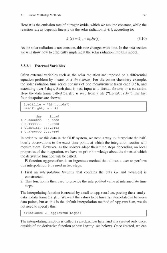
Often external variables such as the solar radiation are imposed on a differentialequation problem by means of a time series. For the ozone chemistry example,the solar radiation time series consists of one measurement taken each 0.5 h, andextending over 5 days. Such data is best input as a data.frame or a matrix.Here the data.frame called Light is read from a file (“Light.rda”); the firstfour datapoints are shown:

load(file = "Light.rda")head(Light, n = 4)

day irrad1 0.0000000 0.00002 0.3333333 0.00003 0.3541667 164.24434 0.3750000 204.7486

In order to use this data in the ODE system, we need a way to interpolate the half-hourly observations to the exact time points at which the integration routine willrequire them. However, as the solvers adapt their time steps depending on localproperties of the integration, we have no prior knowledge about the times at whichthe derivative function will be called.

R function approxfun is an ingenious method that allows a user to performthis interpolation. It is used in two steps:

1. First an interpolating function that contains the data (x- and y-values) isconstructed.

2. This function is then used to provide the interpolated value at intermediate timesteps.

The interpolating function is created by a call to approxfun, passing the x- and y-data in data.frame Light. We want the values to be linearly interpolated in betweendata points, but as this is the default interpolation method of approxfun, we donot need to specify this.

irradiance <- approxfun(Light)

The interpolating function is called irradiance here, and it is created only once,outside of the derivative function (chemistry, see below). Once created, we can


simply call function irradiance with the appropriate time-value to retrieve thesolar radiation at that time. To show that this actually works, the next statementcalculates the irradiances at specific time points (0,0.25,0.5,0.75,1):

irradiance(seq(from = 0, to = 1, by = 0.25))

[1] 0.0000 0.0000 698.8911 490.4644 0.0000

Within the derivative function, we will use irradiance to interpolate the timeseries to the requested time of the simulation (as given by input argument t).

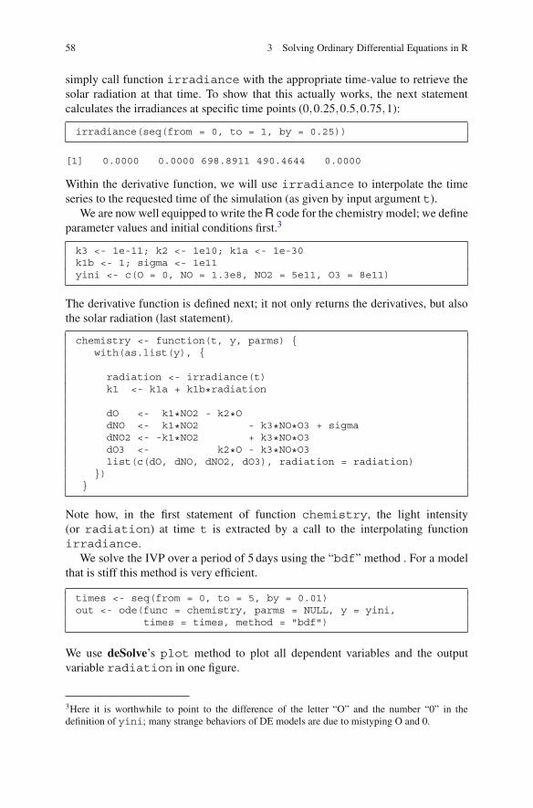
We are now well equipped to write the R code for the chemistry model; we defineparameter values and initial conditions first.3

k3 <- 1e-11; k2 <- 1e10; k1a <- 1e-30k1b <- 1; sigma <- 1e11yini <- c(O = 0, NO = 1.3e8, NO2 = 5e11, O3 = 8e11)

The derivative function is defined next; it not only returns the derivatives, but alsothe solar radiation (last statement).

chemistry <- function(t, y, parms) {with(as.list(y), {

radiation <- irradiance(t)k1 <- k1a + k1b*radiation

dO <- k1*NO2 - k2*OdNO <- k1*NO2 - k3*NO*O3 + sigmadNO2 <- -k1*NO2 + k3*NO*O3dO3 <- k2*O - k3*NO*O3list(c(dO, dNO, dNO2, dO3), radiation = radiation)

})}

Note how, in the first statement of function chemistry, the light intensity(or radiation) at time t is extracted by a call to the interpolating functionirradiance.

We solve the IVP over a period of 5 days using the “bdf” method . For a modelthat is stiff this method is very efficient.

times <- seq(from = 0, to = 5, by = 0.01)out <- ode(func = chemistry, parms = NULL, y = yini,

times = times, method = "bdf")

We use deSolve’s plot method to plot all dependent variables and the outputvariable radiation in one figure.

3Here it is worthwhile to point to the difference of the letter “O” and the number “0” in thedefinition of yini; many strange behaviors of DE models are due to mistyping O and 0.

3.4 Discontinuous Equations, Events 59

0 1 2 3 4 5

0

1000

2000

3000

4000

O

time0 1 2 3 4 5

0e+00

4e+11

8e+11

NO

time0 1 2 3 4 5

0e+00

4e+11

8e+11

NO2

time

0 1 2 3 4 5

4.0e+11

8.0e+11

1.2e+12

O3

time0 1 2 3 4 5

0

200

600

1000

radiation

time

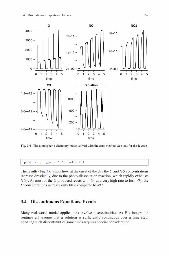
Fig. 3.6 The atmospheric chemistry model solved with the bdf method. See text for the R code

plot(out, type = "l", lwd = 2 )

The results (Fig. 3.6) show how, at the onset of the day the O and NO concentrationsincrease drastically, due to the photo-dissociation reaction, which rapidly exhaustsNO2. As most of the O produced reacts with O2 at a very high rate to form O3, theO concentrations increase only little compared to NO.

3.4 Discontinuous Equations, Events

Many real-world model applications involve discontinuities. As R’s integrationroutines all assume that a solution is sufficiently continuous over a time step,handling such discontinuities sometimes requires special consideration.


There are several levels of difficulty arising in discontinuous model systems.In the simplest case, it is just the forcing or external variables of the systemthat are not smooth. We gave an example of that in the previous section, whereozone degradation depended on light which was prescribed to the model by linearinterpolation between data points.

In this section we give several other examples. The first is a (pharmacokinetic)example of a patient taking a pill every day. This changes the dosing of the drug inthe blood in a discontinuous way. As these discontinuities affect the derivatives ofthe dependent variables they are quite easy to handle.

It is much more difficult to deal with events that cause sudden jumps in the valuesof the dependent variables. This is because the integration methods ignore all directchanges to the state variable values if they occur within the derivative function. Wegive an example of a patient injecting a drug at regular intervals.

In the above two examples, it is known in advance when the change will betriggered, as they occur at preset times. It is even more difficult to deal with suddenchanges that occur only when certain conditions are met. In such cases, a rootfunction is necessary to locate when these conditions arise, after which an eventfunction is called to perform the change. We exemplify this type of discontinuitywith an ODE describing a bouncing ball, and a model that describes temperaturechanges in a heat-controlled room.

Finally, it is not uncommon for solvers that take large steps to miss certainevents. As this leads to wrong solutions, it is important to recognise this, and totake appropriate action to avoid it happening.

3.4.1 Pharmacokinetic Models

In order to be effective, the concentration of a drug taken by a patient must be largeenough, yet too high concentrations may have serious side effects. Pharmacokineticmodels are non-pervasive tools to test the optimal frequency and dosing of drugintake. They represent absorption, distribution, decay and excretion of a drug [21].

Drugs can be dosed orally (pills), or directly injected in the blood. In the firstcase, the action will operate on the processes (absorption through the gut),while inthe latter case, the action will (almost) instantaneously alter the concentration in theblood.

3.4.1.1 A Two-Compartment Model Describing Oral Drug Intake

Consider a patient taking a pill every day at the same time. As the pill passes thegastro-intestinal tract, the drug enters the blood by absorption through the gut wall.The delivery of the drug to the gastro-intestinal tract proceeds for 1 h after which itceases until the next ingestion and so on.


Once in the blood, the drug distributes in the tissues, where it is chemicallyinactivated, so that it can be excreted from the body. An (overly) simple two-compartment model, representing drug concentration in the gut (y1) and in the blood(y2) can represent this process [24]:

y′1 = −ay1 + u(t)y′2 = ay1 − by2.

(3.11)

Here a is the absorption rate, b is the removal rate from the blood, and the term u(t)represents the daily delivery of the drug to the intestinal tract, which we assume tooccur over a period of 1 h.

The discontinuity in this model lies in the dosing of the drug to the intestine(u(t)), which takes a constant value for 1 h, after which it is 0 for the rest of the day.

We now implement the R code for this pharmacokinetic problem. We firstdefine parameters and initial conditions (starting with 0 concentration in boththe intestinal tract and blood) and then implement the derivative function(pharmacokinetics).

As the uptake is periodic, we can use the modulo function (%%) to represent theuptake of the drug:

a <- 6; b <- 0.6yini <- c(intestine = 0, blood = 0)

pharmacokinetics <- function(t, y, p) {if ( (24*t) %% 24 <= 1)

uptake <- 2else

uptake <- 0dy1 <- - a* y[1] + uptakedy2 <- a* y[1] - b *y[2]list(c(dy1, dy2))

}

The problem is solved in the usual way, and its output plotted:

times <- seq(from = 0, to = 10, by = 1/24)out <- ode(func = pharmacokinetics, times = times,

y = yini, parms = NULL)plot(out, lwd = 2, xlab = "day")

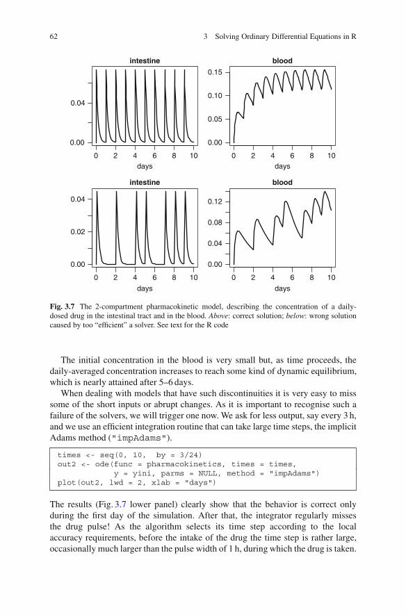
The upper panel of Fig. 3.7 shows the result. At the start of the solution, and foreach first hour of the day, the drug is ingested which causes a steep rise in theintestinal concentrations. As the drug enters the blood, its concentration in theintestine decreases exponentially, while initially increasing in the blood, where itis degraded. Since the inflow to the blood drops exponentially; at a certain point intime loss will exceed input and the concentration in the blood will start to decreaseuntil the next drug dose.


0 2 4 6 8 10

0.00

0.04

intestine

days0 2 4 6 8 10

0.00

0.05

0.10

0.15

blood

days

0 2 4 6 8 10

0.00

0.02

0.04

intestine

days

0 2 4 6 8 10

0.00

0.04

0.08

0.12

blood

days

Fig. 3.7 The 2-compartment pharmacokinetic model, describing the concentration of a daily-dosed drug in the intestinal tract and in the blood. Above: correct solution; below: wrong solutioncaused by too “efficient” a solver. See text for the R code

The initial concentration in the blood is very small but, as time proceeds, thedaily-averaged concentration increases to reach some kind of dynamic equilibrium,which is nearly attained after 5–6 days.

When dealing with models that have such discontinuities it is very easy to misssome of the short inputs or abrupt changes. As it is important to recognise such afailure of the solvers, we will trigger one now. We ask for less output, say every 3 h,and we use an efficient integration routine that can take large time steps, the implicitAdams method ("impAdams").

times <- seq(0, 10, by = 3/24)out2 <- ode(func = pharmacokinetics, times = times,

y = yini, parms = NULL, method = "impAdams")plot(out2, lwd = 2, xlab = "days")

The results (Fig. 3.7 lower panel) clearly show that the behavior is correct onlyduring the first day of the simulation. After that, the integrator regularly missesthe drug pulse! As the algorithm selects its time step according to the localaccuracy requirements, before the intake of the drug the time step is rather large,occasionally much larger than the pulse width of 1 h, during which the drug is taken.


Consequently it may easily miss this pulse until, by chance, it steps into anotherpulse interval.

When this kind of behavior is suspected, it is wise to restrict the size of the timestep. For this particular model, adding argument hmax = 1/24 or using a lowerabsolute tolerance atol = 1e-10 in the call to the ode function will fix theproblem.

3.4.1.2 A One-Compartment Model Describing Drug Injection

In the previous example, uptake of a pill changed the derivative of the intestinal drugconcentration. The differential equations differ when the drug is injected directly inthe blood stream. In this case, the concentration of the drug in the blood is quasi-instantaneously altered, and there is no need to describe the concentration in theintestinal tract. The model that describes the dynamics of the drug in the blood, inbetween injections reads:

b <- 0.6yini <- c(blood = 0)

pharmaco2 <- function(t, blood, p) {dblood <- - b * bloodlist(dblood)

}

Assume a patient who injects daily doses of a drug in her veins, each time increasingthe concentration by 40 units. The injection event causes the value of the statevariable to be altered not the derivative, as in previous example. Unfortunately, thesolvers in deSolve ignore any changes in the state variable values when made in thederivative function, so this is not so simple to implement.

The drug injections have to be specified in a special event data.frame

injectevents <- data.frame(var = "blood",time = 0:20,value = 40,method = "add")

head(injectevents)

var time value method1 blood 0 40 add2 blood 1 40 add3 blood 2 40 add4 blood 3 40 add5 blood 4 40 add6 blood 5 40 add


0 2 4 6 8 10

0

20

40

60

80

blood

days

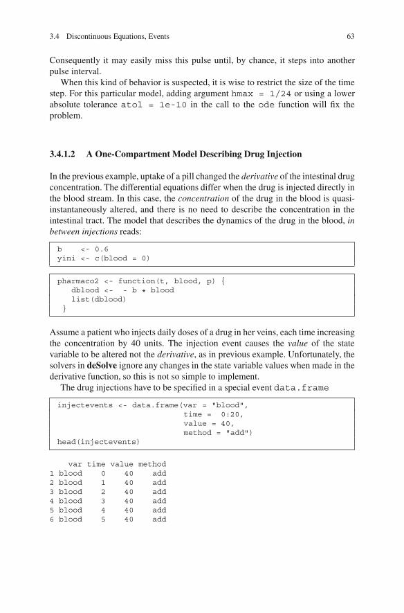
Fig. 3.8 The 1-compartmentpharmacokinetic model,describing the concentrationof a daily-dosed drug injecteddirectly in the blood stream.See text for the R code

The event is said to add the value 40 to the variable blood, at the prescribed time.Other methods of events are to replace with a value, or to multiply with avalue (see “events” help page of the package deSolve; ?events).

When the problem is solved, the existence of an event data.frame is specified bypassing to the solver, a list called events, which contains the data:

times <- seq(from = 0, to = 10, by = 1/24)out2 <- ode(func = pharmaco2, times = times, y = yini,

parms = NULL, method = "impAdams",events = list(data = injectevents))

The results (Fig. 3.8) show the instantaneous adjustment of the concentration in theblood upon injection of the drug, and the exponential decrease in between injections.

plot(out2, lwd = 2, xlab="days")

3.4.2 A Bouncing Ball

In the previous pharmacokinetic examples, it was known in advance when a certainevent was occurring. This allowed us to specify the events in a data.frame(Sect. 3.4.1.2), or to estimate the occurrence based on the simulation time (usingthe modulo function in Sect. 3.4.1.1). The events either consisted of a change in theproblem specification (the derivative), when inputing the drug in the intestinal tract(Sect. 3.4.1.1), or in a change in the value of the state variables when injecting thedrug directly (Sect. 3.4.1.2).

In many cases, we do not know in advance when a certain switch will occur, andlocating this will be part of the solution.

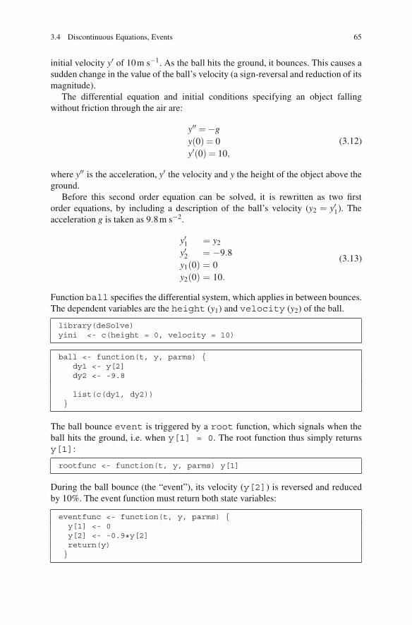
Consider the example of a bouncing ball [25], specified by its position abovethe ground (y). The ball is thrown vertically, from the ground (y(0) = 0), with


initial velocity y′ of 10m s−1. As the ball hits the ground, it bounces. This causes asudden change in the value of the ball’s velocity (a sign-reversal and reduction of itsmagnitude).

The differential equation and initial conditions specifying an object fallingwithout friction through the air are:

y′′ =−gy(0) = 0y′(0) = 10,

(3.12)

where y′′ is the acceleration, y′ the velocity and y the height of the object above theground.

Before this second order equation can be solved, it is rewritten as two firstorder equations, by including a description of the ball’s velocity (y2 = y′1). Theacceleration g is taken as 9.8m s−2.

y′1 = y2

y′2 = −9.8y1(0) = 0y2(0) = 10.

(3.13)

Function ball specifies the differential system, which applies in between bounces.The dependent variables are the height (y1) and velocity (y2) of the ball.

library(deSolve)yini <- c(height = 0, velocity = 10)

ball <- function(t, y, parms) {dy1 <- y[2]dy2 <- -9.8

list(c(dy1, dy2))}

The ball bounce event is triggered by a root function, which signals when theball hits the ground, i.e. when y[1] = 0. The root function thus simply returnsy[1]:

rootfunc <- function(t, y, parms) y[1]

During the ball bounce (the “event”), its velocity (y[2]) is reversed and reducedby 10%. The event function must return both state variables:

eventfunc <- function(t, y, parms) {y[1] <- 0y[2] <- -0.9*y[2]return(y)}


0

0

5 10 15 20

1

2

3

4

5

bouncing ball

time

heig

ht

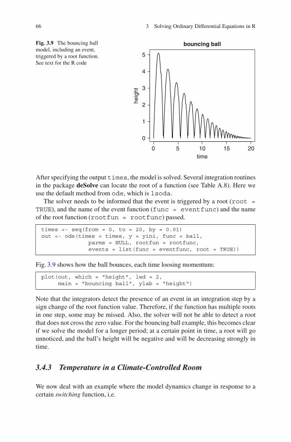
Fig. 3.9 The bouncing ballmodel, including an event,triggered by a root function.See text for the R code

After specifying the output times, the model is solved. Several integration routinesin the package deSolve can locate the root of a function (see Table A.8). Here weuse the default method from ode, which is lsoda.

The solver needs to be informed that the event is triggered by a root (root =TRUE), and the name of the event function (func = eventfunc) and the nameof the root function (rootfun = rootfunc) passed.

times <- seq(from = 0, to = 20, by = 0.01)out <- ode(times = times, y = yini, func = ball,

parms = NULL, rootfun = rootfunc,events = list(func = eventfunc, root = TRUE))

Fig. 3.9 shows how the ball bounces, each time loosing momentum:

plot(out, which = "height", lwd = 2,main = "bouncing ball", ylab = "height")

Note that the integrators detect the presence of an event in an integration step by asign change of the root function value. Therefore, if the function has multiple rootsin one step, some may be missed. Also, the solver will not be able to detect a rootthat does not cross the zero value. For the bouncing ball example, this becomes clearif we solve the model for a longer period; at a certain point in time, a root will gounnoticed, and the ball’s height will be negative and will be decreasing strongly intime.

3.4.3 Temperature in a Climate-Controlled Room

We now deal with an example where the model dynamics change in response to acertain switching function, i.e.


y′ = f1(x) if g(x) = 1y′ = f2(x) if g(x) = 0,

(3.14)

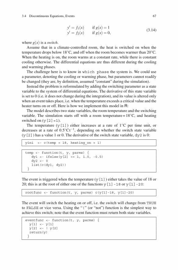
where g(x) is a switch.Assume that in a climate-controlled room, the heat is switched on when the

temperature drops below 18◦C, and off when the room becomes warmer than 20◦C.When the heating is on, the room warms at a constant rate, while there is constantcooling otherwise. The differential equations are thus different during the coolingand warming phases.

The challenge here is to know in which phase the system is. We could usea parameter, denoting the cooling or warming phase, but parameters cannot readilybe changed (they are, by definition, assumed “constant” during the simulation).

Instead the problem is reformulated by adding the switching parameter as a statevariable to the system of differential equations. The derivative of this state variableis set to 0 (i.e. it does not change during the integration), and its value is altered onlywhen an event takes place, i.e. when the temperature exceeds a critical value and theheater turns on or off. Here is how we implement this model in R:

The model describes two state variables, the room temperature and the switchingvariable. The simulation starts off with a room temperature = 18◦C, and heatingswitched on (y[2]=1).

The temperature (y[1]) either increases at a rate of 1◦C per time unit, ordecreases at a rate of 0.5◦Ct−1, depending on whether the switch state variable(y[2]) has a value 1 or 0. The derivative of the switch state variable, dy2 is 0:

yini <- c(temp = 18, heating_on = 1)

temp <- function(t, y, parms) {dy1 <- ifelse(y[2] == 1, 1.0, -0.5)dy2 <- 0list(c(dy1, dy2))

}

The event is triggered when the temperature (y[1]) either takes the value of 18 or20; this is at the root of either one of the functions y[1]-18 or y[1]-20:

rootfunc <- function(t, y, parms) c(y[1]-18, y[1]-20)

The event will switch the heating on or off, i.e. the switch will change from TRUEto FALSE or vice versa. Using the “!” (or “not”) function is the simplest way toachieve this switch; note that the event function must return both state variables.

eventfunc <- function(t, y, parms) {y[1] <- y[1]y[2] <- ! y[2]return(y)}


0 5 10 15 20

18.0

18.5

19.0

19.5

20.0

temp

time

0 5 10 15 20

0.0

0.2

0.4

0.6

0.8

1.0

heating_on

time

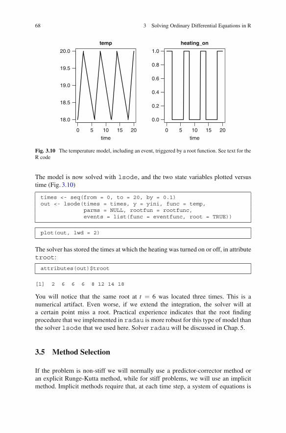
Fig. 3.10 The temperature model, including an event, triggered by a root function. See text for theR code

The model is now solved with lsode, and the two state variables plotted versustime (Fig. 3.10)

times <- seq(from = 0, to = 20, by = 0.1)out <- lsode(times = times, y = yini, func = temp,

parms = NULL, rootfun = rootfunc,events = list(func = eventfunc, root = TRUE))

plot(out, lwd = 2)

The solver has stored the times at which the heating was turned on or off, in attributetroot:

attributes(out)$troot

[1] 2 6 6 6 8 12 14 18

You will notice that the same root at t = 6 was located three times. This is anumerical artifact. Even worse, if we extend the integration, the solver will ata certain point miss a root. Practical experience indicates that the root findingprocedure that we implemented in radau is more robust for this type of model thanthe solver lsode that we used here. Solver radau will be discussed in Chap. 5.

3.5 Method Selection

If the problem is non-stiff we will normally use a predictor-corrector method oran explicit Runge-Kutta method, while for stiff problems, we will use an implicitmethod. Implicit methods require that, at each time step, a system of equations is

3.5 Method Selection 69

solved to give the required solution (see Sect. 2.6). If the problem is stiff and linearthen the algebraic equations to be solved are linear. In contrast, nonlinear equationsare typically solved iteratively, using a variant of Newton’s method [20]. Thisleads to a linear algebraic problem involving the Jacobian matrix at each iteration,and therefore multiple function evaluations per time step. Although in practice,the Jacobian will not be inverted (this is very inefficient), but rather Gaussianelimination will be used, this still requires quite a lot of computational overhead.On the other hand, as these multistep methods use previously computed values toevaluate the values at the next time step, they can attain high order of accuracy inless steps than taken by explicit methods, such as Runge-Kutta methods. The trade-off between number of steps and number of function evaluations per step, versusthe overhead induced by the calculations involving the Jacobian determine whichmethod is most efficient for a particular problem.

It will soon become very clear if we choose the wrong method. For instance,if an explicit method is chosen to solve a stiff problem, very small time stepswill be taken in order to maintain stability, and it will take a long time to solvethe problem. In such cases, the implicit bdf methods will be able to take muchlarger steps and solve the problem in a fraction of the time. In contrast, for non-stiff methods, the computational burden of Jacobian evaluation may overwhelmthe fewer function evaluations needed. This is especially the case for very largesets of equations (e.g. resulting from numerically approximating partial differentialequations, see Chap. 8), which, if they do not generate a stiff problem, may be muchmore efficiently solved with an explicit method.

It is generally not clear in advance which method may be best suited for aparticular problem, but as using the optimal method may significantly improveoverall performance, we give some rules of thumb to aid in the selection of themost appropriate method:

1. Use an implicit method only if the ODE problem is stiff; bdf, radau, mebdfi,gamd or bimd are best suited for very stiff problems, the adams methodsfor mildly stiff problems. The latter may also be more efficient for non-stiffproblems, although the explicit Runge-Kutta methods are contenders in thesecases.

2. If it is not known whether a problem is stiff, then use lsoda from the packagedeSolve or dopri5, cashkarp or dopri853 from the package deTestSet toprint when problems become stiff. To provoke the printing of these features, setargument verbose=TRUE.

3. The diagnostics of a solution generated by the solvers provide a user withinformation about the number of function evaluations, and, for implicit methods,of the number of Jacobian decompositions. The diagnostics of methodlsodawill tell the user which method was used, and when lsoda has switchedbetween methods during the simulation.

4. Performance can be readily assessed by timing a model solution, using R’sfunction system.time()method. So, as a crude approach, we can try severalmethods and simply take the one that requires least simulation time with a similar


accuracy (work precision diagrams described in Sect. 3.5.1.3 are very useful forthis purpose).

5. We can also assess performance by recording the number of function or Jacobianevaluations.

3.5.1 The van der Pol Equation

A commonly used example to demonstrate stiffness is the van der Pol problem (see[11]). It is defined by the following second order differential equation:

y′′ − μ(1− y2)y′+ y = 0, (3.15)

where μ is a parameter. We convert (3.15) in a first order system of ODEs by addingan extra variable, representing the first order derivative:

y′1 = y2

y′2 = μ(1− y21)y2 − y1.

(3.16)

Stiff problems are obtained for large μ , non-stiff for small μ ; the problems haveboth stiff and non-stiff parts for intermediate values of the parameter. We run themodel for μ = 1, 10, 1000, and using ode as the integrator:

yini <- c(y = 2, dy = 0)Vdpol <- function(t, y, mu)

list(c(y[2],mu * (1 - y[1]ˆ2) * y[2] - y[1]))

times <- seq(from = 0, to = 30, by = 0.01)nonstiff <- ode(func = Vdpol, parms = 1, y = yini,

times = times, verbose = TRUE)interm <- ode(func = Vdpol, parms = 10, y = yini,

times = times, verbose = TRUE)stiff <- ode(func = Vdpol, parms = 1000, y = yini,

times =0:2000, verbose = TRUE)

3.5.1.1 Printing the Diagnostics of the Solutions

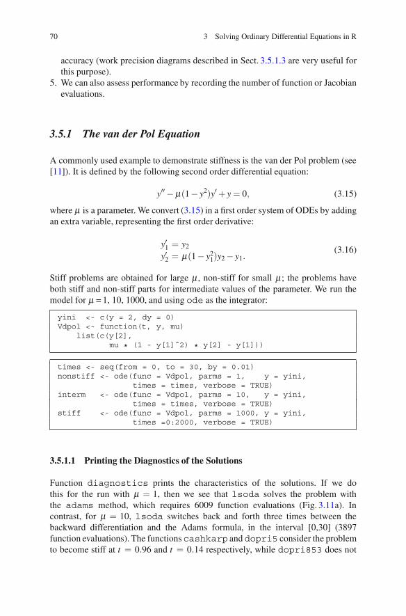
Function diagnostics prints the characteristics of the solutions. If we dothis for the run with μ = 1, then we see that lsoda solves the problem withthe adams method, which requires 6009 function evaluations (Fig. 3.11a). Incontrast, for μ = 10, lsoda switches back and forth three times between thebackward differentiation and the Adams formula, in the interval [0,30] (3897function evaluations). The functionscashkarp and dopri5 consider the problemto become stiff at t = 0.96 and t = 0.14 respectively, while dopri853 does not


0 5 10 15 20 25 30

−2

−1

0

1

2mu=1

time

ya b

c

0 5 10 15 20 25 30

−2

−1

0

1

2mu=10

time

y

0 500 1000 1500 2000

−2

−1

0

1

2mu=1000

time

y stiff − bdfnonstiff − adams

van der Pol equation

Fig. 3.11 Three solutions of the van der Pol equation, solved with method lsoda. The regionswhere the solver uses the adams or the backward differentiation formula are indicated

consider this problem to be stiff. Method switching by lsoda also occurs twicewhen μ = 1000, in the time interval [0, 2000] but here the region where the non-stiff method is used is very narrow (the thin grey line in Fig. 3.11c).

diagnostics(nonstiff)

--------------------lsoda return code--------------------

return code (idid) = 2Integration was successful.

--------------------INTEGER values--------------------

1 The return code : 22 The number of steps taken for the problem so far: 30043 The number of function evaluations for the problem so far: 6009


5 The method order last used (successfully): 76 The order of the method to be attempted on the next step: 77 If return flag =-4,-5: the largest component in error vector 08 The length of the real work array actually required: 529 The length of the integer work array actually required: 22

14 The number of Jacobian evaluations and LU decompositions so far: 015 The method indicator for the last succesful step,

1=adams (nonstiff), 2= bdf (stiff): 116 The current method indicator to be attempted on the next step,

1=adams (nonstiff), 2= bdf (stiff): 1

--------------------RSTATE values--------------------

1 The step size in t last used (successfully): 0.012 The step size to be attempted on the next step: 0.013 The current value of the independent variable which the solver hasreached: 30.00947

4 Tolerance scale factor > 1.0 computed when requesting too muchaccuracy: 0

5 The value of t at the time of the last method switch, if any: 0

3.5.1.2 Timings

We can also run the same model with different integrators, each time printing thetime it takes (in seconds) to solve the problem:

library(deTestSet)system.time(ode(func = Vdpol, parms = 10, y = yini,

times = times, method = "ode45") )


system.time(ode(func = Vdpol, parms = 10, y = yini,times = times, method = "adams"))


system.time(ode(func = Vdpol, parms = 10, y = yini,times = times, method = "bdf"))


system.time(radau(func = Vdpol, parms = 10, y = yini,times = times))



system.time(bimd(func = Vdpol, parms = 10, y = yini,times = times))


system.time(mebdfi(func = Vdpol, parms = 10, y = yini,times = times))


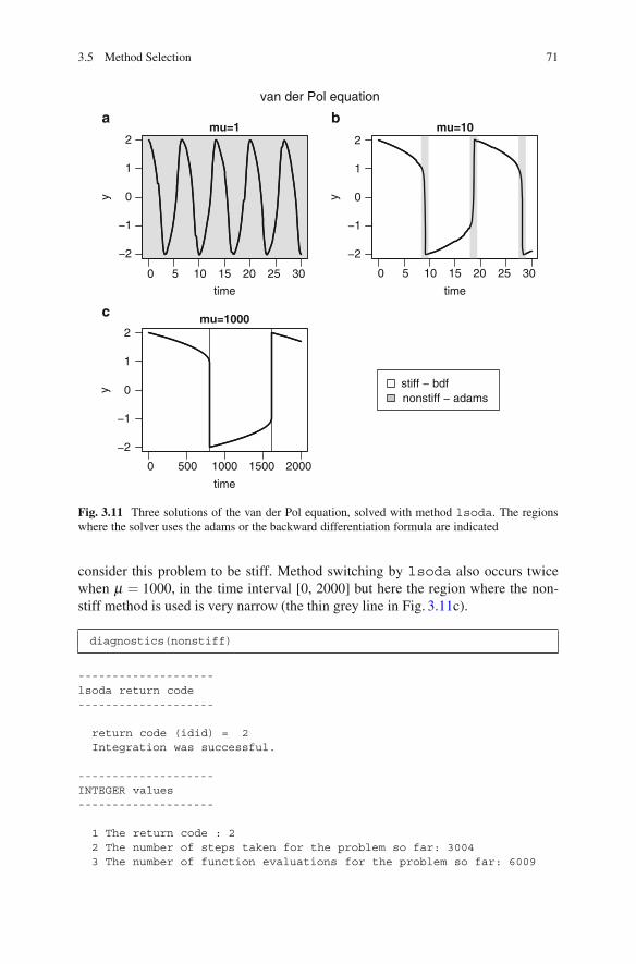
We ran the van der Pol problem with a number of different integration methods,each time using diagnostics to write the number of steps, function evaluations,Jacobian matrix decompositions and method switches performed by the integrators.Results are in Table 3.1. Clearly, the adams method which is most efficientfor solving the non-stiff problem (requires fewest function evaluations), becomescompletely unsuited in the stiff case, requiring more than eight million functionevaluations! The implicit methods (lsoda, bdf, impAdams, mebdfi) per-form rather well in all cases.

Table 3.1 Performance of various integration routines implemented in deSolve, based on the vander Pol equation with different values of parameter μMethod Steps Function Jacobian Switches to

evaluations evaluations adams

times=seq(0,30,0.1) μ = 1

lsoda 528 1173 0 0bdf 789 1070 64adams 675 744 0impAdams 539 811 55rk45ck 300 1802 0mebdfi 659 2439 71

times=seq(0,30,0.1) μ = 10


times=0:2000 μ = 1,000



4 6 8 10 12

0.02

0.05

0.10

0.20

0.50mu = 1

mescd

seco

nds

elap

sed

lsodabdfimpAdamsmebdfigamdradau

a

0 2 4 6 8

0.1

0.2

0.5

mu = 1000

mescd

seco

nds

elap

sed

lsodabdfimpAdamsmebdfigamdradau

b

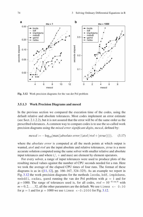
Fig. 3.12 Work precision diagrams for the van der Pol problem

3.5.1.3 Work Precision Diagrams and mescd

In the previous section we compared the execution time of the codes, using thedefault relative and absolute tolerances. Most codes implement an error estimate(see Sect. 2.1.2.2), but it is not assured that the error will be of the same order as theprescribed tolerances. A common way to compare codes is to use the so-called workprecision diagrams using the mixed error significant digits, mescd, defined by:

mescd :=− log10(max(|absolute error/(atol/rtol+ |ytrue|)|)), (3.17)

where the absolute error is computed at all the mesh points at which output iswanted, atol and rtol are the input absolute and relative tolerances, ytrue is a moreaccurate solution computed using the same solver with smaller relative and absoluteinput tolerances and where (/, + and max) are element by element operators.

For every solver, a range of input tolerances were used to produce plots of theresulting mescd values against the number of CPU seconds needed for a run. Herewe took the average of the elapsed CPU times of four runs. The format of thesediagrams is as in ([11, 12], pp. 166–167, 324–325). As an example we report inFig. 3.12 the work precision diagrams for the methods lsoda, bdf, impAdams,mebdfi, radau, gamd running the van der Pol problem with μ = 1 and forμ =1000. The range of tolerances used is, for all codes, rtol = 10−4+m/4 withm = 0,2, . . . ,32, all the other parameters are the default. We use times <- 0:30for μ = 1 and for μ = 1000 we use times <-0:2000 for Fig. 3.12.

3.6 Exercises 75

We want to emphasize that the reader should be careful when using thesediagrams for a mutual comparison of the solvers. The diagrams just show the resultof runs with the prescribed input on the specified computer. A more sophisticatedsetting of the input parameters, another computer or compiler, as well as anotherrange of tolerances, or even another choice of the input vector times may changethe diagrams considerably (not shown). For the van der Pol problem for μ = 1the impAdams is the most efficient code (Fig. 3.12a), while for μ = 1000 lsodaand bdf require the least computational time to compute a solution with a similarnumber of mescd (Fig. 3.12b).

3.6 Exercises

3.6.1 Getting Started with IVP

Solve the problem

y′ = y2 + t, (3.18)

with initial condition y(0)= 0.1 on the interval [0,1]; write the output to matrix out.Now solve the following equations

y′ = y2 − yt, (3.19)

andy′ = y2 + 1, (3.20)

with the same initial condition, and same output times. Save the output of theproblems (3.19) and (3.20) to matrices out2, and out3 respectively. Plot theoutput of the three models in one plot.

Solve the following second order equation for t ∈ [0,20].

y′′ =−0.1y. (3.21)

The initial conditions are y(0) = 1, y′(0) = 0. You will first need to rewritethis equation as two first order equations. Finally, solve the following differentialproblem using ode45

y′′+ 2y′+ 3y = cos(t)

y(0) = y′(0) = 0, (3.22)

in the interval [0,2π].


3.6.2 The Robertson Problem

This is a stiff problem consisting of three ordinary differential equations. It describesthe kinetics of an autocatalytic reaction given by [22]. The equations are:

y′1 =−k1y1 + k3y2y3

y′2 = k1y1 − k2y22 − k3y2y3

y′3 = k2y22. (3.23)

Solve the problem in R; use as initial conditions y1 = 1, y2 = 0, y3 = 0. The valuesfor the parameters are k1 = 0.04; k2 = 3.107; k3 = 1.104. First integrate the problemon the interval 0 ≤ t ≤ 40. Then integrate it in the interval 10−4 ≤ t ≤ 107.

Use for the second output times a logarithmic series:

times <- 10ˆ(seq(from = -4, to = 7, by = 0.1))

When plotting the outcome, scale the x-axis logarithmically.

3.6.3 Displaying Results in a Phase-Plane Graph

In (Sect. 3.2.1) the results of a three-equation model, the rigid body model, weredisplayed in a 3D phase plane, using the R package scatterplot3D.

3.6.3.1 The Rossler Equations

Produce a 3-D phase-plane plot of the following set of ODEs, which you solve onthe interval [0, 100] and with initial conditions equal to (1, 1, 1):

y′1 =−y2 − y3

y′2 = y1 + ay2

y′3 = b+ y3(y1 − c), (3.24)

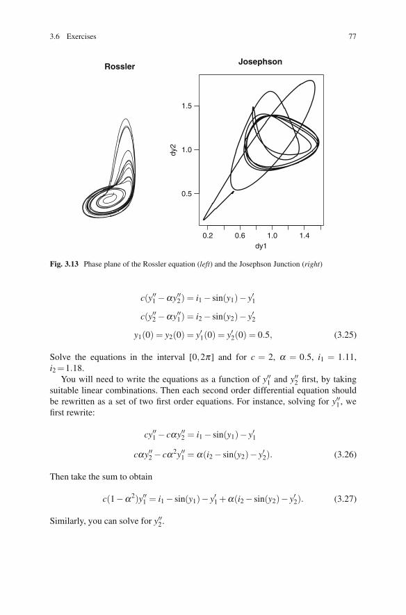
for a = 0.2, b = 0.2, c = 5. This system, called the Rossler equations, is due to [23];its output is in Fig. 3.13, left (use ?scatterplot3d to find out how to get rid ofthe axis and grid).

3.6.3.2 Josephson Junctions

The next example, again from [12] describes superconducting Josephson Junctions.The equations are:

3.6 Exercises 77

Rossler

0.2 0.6 1.0 1.4

0.5

1.0

1.5

Josephson

dy1

dy2

Fig. 3.13 Phase plane of the Rossler equation (left) and the Josephson Junction (right)

c(y′′1 −αy′′2) = i1 − sin(y1)− y′1

c(y′′2 −αy′′1) = i2 − sin(y2)− y′2

y1(0) = y2(0) = y′1(0) = y′2(0) = 0.5, (3.25)

Solve the equations in the interval [0,2π] and for c = 2, α = 0.5, i1 = 1.11,i2=1.18.

You will need to write the equations as a function of y′′1 and y′′2 first, by takingsuitable linear combinations. Then each second order differential equation shouldbe rewritten as a set of two first order equations. For instance, solving for y′′1, wefirst rewrite:

cy′′1 − cαy′′2 = i1 − sin(y1)− y′1

cαy′′2 − cα2y′′1 = α(i2 − sin(y2)− y′2). (3.26)

Then take the sum to obtain

c(1−α2)y′′1 = i1 − sin(y1)− y′1 +α(i2 − sin(y2)− y′2). (3.27)

Similarly, you can solve for y′′2.


0 5 10 15 20

2

4

6

8

10

y

time

unharvested2−day harvestharvest at 80% of K

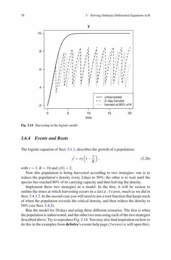
Fig. 3.14 Harvesting in the logistic model

3.6.4 Events and Roots

The logistic equation of Sect. 3.1.1, describes the growth of a population:

y′ = ry(

1− yK

), (3.28)

with r = 1, K = 10 and y(0) = 2.Now this population is being harvested according to two strategies: one is to

reduce the population’s density every 2 days to 50%; the other is to wait until thespecies has reached 80% of its carrying capacity and then halving the density.

Implement these two strategies in a model. In the first, it will be easiest tooutline the times at which harvesting occurs in a data.frame, much as we did inSect. 3.4.1.2. In the second case you will need to use a root function that keeps trackof when the population exceeds the critical density, and then reduce the density to50% (see Sect. 3.4.2).

Run the model for 20 days and using three different scenarios. The first is whenthe population is unharvested, and the other two runs using each of the two strategiesdescribed above. Try to reproduce Fig. 3.14. You may also find inspiration on how todo this in the examples from deSolve’s events help page (?events will open this).

References 79

3.6.5 Stiff Problems

Several stiff test problems are described in [27]. One of their problems, calledds1ode, is given by:

y′ =−σ(y3 − 1), (3.29)

where σ is a parameter that determines the stiffness of the problem. Solve theproblem in the interval [0, 10], with y(0) = 1.2 and for three values of σ , equalto 106, 1 and 10−1. Plot the three outputs in the same figure. Use functiondiagnostics to see how the integration was done (number of steps, methodselected, etc. . . ).

References

1. Arenstorf, R. F. (1963). Periodic solutions of the restricted three-body problem representinganalytic continuations of Keplerian elliptic motions. American Journal of Mathematics, 85,27–35.

2. Aris, R. (1965). Introduction to the analysis of chemical reactors. Englewood Cliffs: PrenticeHall.

3. Bogacki, P., & Shampine, L. F. (1989). A 3(2) pair of Runge–Kutta formulas. AppliedMathematics Letters, 2, 1–9.

4. Brown, P. N., Byrne, G. D., & Hindmarsh, A. C. (1989). VODE, a variable-coefficient ODEsolver. SIAM Journal on Scientific and Statistical Computing, 10, 1038–1051.

5. Brugnano, L., & Magherini, C. (2004). The BiM code for the numerical solution of ODEs.Journal of Computational and Applied Mathematics, 164–165, 145–158.

6. Cash, J. R., & Considine, S. (1992). An MEBDF code for stiff initial value problems. ACMTransactions on Mathematical Software, 18(2), 142–158.

7. Cash, J. R., & Karp, A. H. (1990). A variable order Runge–Kutta method for initial valueproblems with rapidly varying right-hand sides. ACM Transactions on Mathematical Software,16, 201–222.

8. Dormand, J. R., & Prince, P. J. (1980). A family of embedded Runge–Kutta formulae. Journalof Computational and Applied Mathematics, 6, 19–26.

9. Dormand, J. R., & Prince, P. J. (1981). High order embedded Runge–Kutta formulae. Journalof Computational and Applied Mathematics, 7, 67–75.

10. Fehlberg, E. (1967). Klassische Runge–Kutta formeln funfter and siebenter ordnung mitschrittweiten-kontrolle. Computing (Arch. Elektron. Rechnen), 4, 93–106.

11. Hairer, E., & Wanner, G. (1996). Solving ordinary differential equations II: Stiff anddifferential-algebraic problems. Heidelberg: Springer.

12. Hairer, E., Norsett, S. P., & Wanner, G. (2009). Solving ordinary differential equationsI: Nonstiff problems (2nd rev. ed.). Heidelberg: Springer.

13. Hindmarsh, A. C. (1980). LSODE and LSODI, two new initial value ordinary differentialequation solvers. ACM-SIGNUM Newsletter , 15, 10–11.

14. Hindmarsh, A. C. (1983). ODEPACK, a systematized collection of ODE solvers. InR. Stepleman (Ed.), Scientific computing: Vol. 1. IMACS transactions on scientific computation(pp. 55–64). Amsterdam: IMACS/North-Holland.

15. Hundsdorfer, W., & Verwer, J. G. (2003). Numerical solution of time-dependent advection-diffusion-reaction equations. Springer series in computational mathematics. Berlin: Springer.


16. Iavernaro, F., & Mazzia, F. (1998). Solving ordinary differential equations by generalizedAdams methods: Properties and implementation techniques. Applied Numerical Mathematics,28(2–4), 107–126. Eighth conference on the numerical treatment of differential equations(Alexisbad, 1997).

17. Ligges, U., & Machler, M. (2003). Scatterplot3d–an R package for visualizing multivariatedata. Journal of Statistical Software, 8(11), 1–20.

18. Lorenz, E. N. (1963). Deterministic non-periodic flows. Journal of Atmospheric Sciences, 20,130–141.

19. Petzold, L. R. (1983). Automatic selection of methods for solving stiff and nonstiff systemsof ordinary differential equations. SIAM Journal on Scientific and Statistical Computing, 4,136–148.

20. Press, W. H., Teukolsky, S. A., Vetterling, W. T., & Flannery, B. P. (2007). Numerical recipes(3rd ed). Cambridge: Cambridge University Press.

21. Reddy, M., Yang, R. S., Andersen, M. E., & Clewell, H. J., III (2005). Physiologically basedpharmacokinetic modeling: Science and applications. Hoboken: Wiley.

22. Robertson, H. H. (1966). The solution of a set of reaction rate equations. In J. Walsh (Ed.),Numerical analysis: An introduction (pp. 178–182). London: Academic Press.

23. Rossler, O. E. (1976). An equation for continous chaos. Physics Letters A, 57(5), 397–398.24. Shampine, L. F. (1994). Numerical solution of ordinary differential equations. New York:

Chapman and Hall.25. Shampine, L. F., Gladwell, I., & Thompson, S. (2003). Solving ODEs with MATLAB.

Cambridge: Cambridge University Press.26. Soetaert, K., Petzoldt, T., & Setzer, R. W. (2010). Solving differential equations in R: Package

deSolve. Journal of Statistical Software, 33(9), 1–25.27. van Dorsselaer, J. L. M., & Spijker, M. N. (1994). The error committed by stopping the newton

iteration in the numerical solution of stiff initial value problems. IMA journal of NumericalAnalysis, 14, 183–209.

28. Verhulst, P. (1838). Notice sur la loi que la population poursuit dans son accroissement.Correspondance Mathematique et Physique, 10, 113–121.

http://www.springer.com/978-3-642-28069-6

Chapter 3 Solving Ordinary Differential Equations in R

Documents

Transcript of Chapter 3 Solving Ordinary Differential Equations in R