Chapter 3 Quanto Multiple-reset Options
25
18 Chapter 3 Quanto Multiple-reset Options 3.1 Framework The content of this chapter is as follows: 3.2 is the price and risk analysis of Type I quanto multiple-reset option; 3.3 is the price and risk analysis of Type II quanto multiple-reset option; 3.4 is the price and risk analysis of Type III quanto multiple-reset option; 3.5 is the price and risk analysis of Type IV quanto multiple-reset option. 3.2 Price and Risk Analysis of Type I Quanto Multiple-reset Option 3.2.1 Pricing Model First of all, we interpret the final payoff of the Type I quanto multiple-reset put. Let { } 1 2 , ,..., n tt t is the date at which the exercise price will be resetted, called the reset date, and 1 n T t + = , which is the maturity of this put. ( ) I QRP T represents the final payoff of the Type I quanto multiple-reset put, which can be written as follows: In which, The Type I quanto multiple-reset put is the multiple-reset put whose final value is computed in foreign currency first at the maturity date, and transferred into the value denominated in domestic currency by the current exchange rate. Consequently, this kind of quanto multiple-reset put is suitable for the investor who invests their money in foreign stocks and pays more attention to the risk of the foreign stock price than the exchange rate. Based on the definition of the final payoff in Eq(3- 1) and (3- 2), we can use the Martingale Pricing method to price the fair price of the Type I quanto multiple-reset { } ( ) () ( ) ( ),0 I n QRP T XT Max K t ST = ⋅ - (3- 1) 1 1 ( ) (( ), ( ),..., ( ), ) n n n Kt Max S t St St K - = (3- 2)
Transcript of Chapter 3 Quanto Multiple-reset Options
18
Chapter 3 Quanto Multiple-reset Options
3.1 Framework
The content of this chapter is as follows: 3.2 is the price and risk analysis of Type
I quanto multiple-reset option; 3.3 is the price and risk analysis of Type II quanto
multiple-reset option; 3.4 is the price and risk analysis of Type III quanto
multiple-reset option; 3.5 is the price and risk analysis of Type IV quanto
multiple-reset option.
3.2 Price and Risk Analysis of Type I Quanto Multiple-reset Option
3.2.1 Pricing Model
First of all, we interpret the final payoff of the Type I quanto multiple-reset put.
Let { }1 2, ,..., nt t t is the date at which the exercise price will be resetted, called the
reset date, and 1nT t += , which is the maturity of this put. ( )IQRP T represents the
final payoff of the Type I quanto multiple-reset put, which can be written as follows:
In which,
The Type I quanto multiple-reset put is the multiple-reset put whose final value is
computed in foreign currency first at the maturity date, and transferred into the value
denominated in domestic currency by the current exchange rate. Consequently, this
kind of quanto multiple-reset put is suitable for the investor who invests their money
in foreign stocks and pays more attention to the risk of the foreign stock price than the
exchange rate.
Based on the definition of the final payoff in Eq(3- 1) and (3- 2), we can use the
Martingale Pricing method to price the fair price of the Type I quanto multiple-reset
{ }( ) ( ) ( ) ( ),0I
nQRP T X T Max K t S T= ⋅ − (3- 1)
1 1( ) ( ( ), ( ),..., ( ), )n n nK t Max S t S t S t K−= (3- 2)
19
put as follows:13
In which, ( )dN ⋅ represents the d-dimensional cdf of joint stndard normal,
iA∑ represents each of the correlation matrix in the d-dimensional cdf of joint
stndard normal. All the parameters in Eq(3- 3) are illustrated as follows:
1
2
( )( )2 ,
sf j i
A
j
s j i
r t t
d i jt t
σ
σ
− −= <
− (3- 4)
2
2
0ln( ) ( )2
sf i
A
K
s i
Sr t
Kdt
σ
σ
+ +=
(3- 5)
2
2
( )( )2 ,
sf i h
A
h
s i h
r t t
d h it t
σ
σ
+ −= <
−
(3- 6)
3
2
( )( )2 ,
sf j i
A
j
s j i
r t t
d i jt t
σ
σ
+ −= <
− (3- 7)
4
2
0ln( ) ( )2
sf j
A
j
s j
Sr t
Kdt
σ
σ
+ −= (3- 8)
13 The detailed derivation is illustrated in Appendix A.
2 2 2
2
1 1
1
3 3
3
4 4
4
5
1 1
( )0 0 0 1 1 1
1
1 1 1
1 1 1
0
0 1 1
( , , ..., ; )
( , ..., ; )
( , ..., ; )
( , ..., ; )
( , ...,
f i
f
A A A
i k i A
nI r T t A A
n i i n Ai
A A
n i i n A
r T A A
n n A
A
n
N d d d
QRP X S e N d d
N d d
Ke N d dX
S N d
−
− −
− + + +=
− + + +
−
+ +
+
∑ ⋅ = ⋅ − − ∑ − − − ∑
⋅ − − ∑+
− − −
∑
5
51; )A
n Ad +
∑
(3- 3)
20
5
2
0ln( ) ( )2
sf j
A
j
s j
Sr t
Kdt
σ
σ
+ += (3- 9)
1 1
2 1
1 2
2 1
1 2
1 1
1 3
1 ...
1 ...
1
i i i i
i i n i
i i i i
i i n i
i i i i
n i n i
A A
t t t t
t t t t
t t t t
t t t t
t t t t
t t t t
+ +
+ +
+ +
+ +
+ +
+ +
− −
− −
− − = = − −
− − − −
∑ ∑
M M O M
L
(3- 10)
1 1
1 1
2
1 1
1
2
1
1
1
i i i
i i
i i i
i i
i i i i
i i
A
t t t t
t t
t t t t
t t t
t t t t
t t t
−
−
− −
− −
− − = −
− − −
∑
L
L
M M O M
L
(3- 11)
1 1
2 1
1 2
2 1
1 2
1 1
54
1
1
1
n
n
n n
A A
t t
t t
t t
t t
t t
t t
+
+
+ +
= =
∑ ∑
L
L
M M O M
L
(3- 12)
If we let 1n = , the reset date be 0t and the maturity of the put be 1nT t += and
put them back into Eq(3- 3), we’ll have the pricing formula of the Type I quanto
single-reset put as follows:
We can compare the Eq(3- 13) with the result in Jiang(2004), and we can find
0 32 1
4 4
4
5 5
5
( )
0 0 0 2 2
2 1 2
0
0 2 1 2
( ) ( ) ( )
( , ; )
( , ; )
f
f
r T t AA AI
k
r T A A
A
A A
A
QRP X S N d e N d N d
Ke N d dX
S N d d
− −
−
= ⋅ ⋅ − − −
⋅ − − ∑ +
− − − ∑
(3- 13)
21
the two pricing formulas are consistent.
On the other hand, we can rewrite Eq(3- 3) as follows:
Based on Eq(3- 14), we can find that the Type I quanto multiple-reset put( IQRP )
is composed of the n units of Contingent Forward-Start Put14 and a conditional
quanto put15. In order to more easily explain how the 2 kinds of options affect the
Type I quanto multiple-reset put, we take a numerical example to illustrate it.
We assume that there exist two kinds of Type I quanto reset option with exercise
price both equal to 5 and whose maturity dates are both the day after three months.
One of them is a Type I quanto single-reset option whose reset date is the day after a
month, represented by *
IQRP . The other one is a Type I quanto double-reset option
whose reset date is the last day of the first and second month, represented by IQRP .
The domestic and foreign risk-free rates are 1.5% and 4.5%. The initial price of the
foreign stock and exchange rate are 5 and 32.5. The data of the volatility of the
foreign stock and exchange rate are as follows: 50%Sσ = , 35%Xσ = , , 0.5S Xρ = . We
substitute all of the parameters we assume into Eq(3- 13), Eq(3- 3)~(3- 12) and Eq(2-
14 That is
I
AiQRP .
15 That is I
BQRP .
2 2 2
2
1 1
1
3 32 2 2
2 3
( )
0 1 1
1 1 10 0
0 1 1 1 1 1
( , , ..., ; )
( , ..., ; )
( , , ..., ; ) ( , ..., ; )
f i
IAi
r T t A A A
i k i A
A AI
n i i n A
A AA A A
i k i A n i i n A
QRP
S e N d d d
N d dQRP X
S N d d d N d d
− −
−
− + + +
− − + + +
∑ ⋅ − − − ∑= ∑ ⋅ − − ∑ 144444444444424444444444 3
( ) { }{ }
4 4
4
5 5
5
1
1
1 1 1
0
0 1 1 1
1
{ ( ) ( ),..., ( ), }
( , ..., ; )
( , ..., ; )
( ) ( ( ) ( )
f
IB
i n
IAi
n
i
r T A A
n n A
A A
n n A
QRP
nI I
Ai B
i
rT Q
i S t Max S t S t K
QRP
Ke N d dX
S N d d
QRP QRP
e E X T S t S T I
=
−
+ +
+ +
=
+−
=
⋅ − − ∑ +
− − − ∑
= +
= ⋅ − ⋅
∑
∑
44
14444444244444443
144444444442444 3
( ) { }{ }1
1
{ ( ),..., ( ), }( ) ( ( )
n
IB
n
i
rT Q
K Max S t S t K
QRP
e E X T K S T I
=
+−
=+ ⋅ − ⋅
∑4444444
144444444424444444443
(3- 14)
22
15) to find the fair price of the Type I quanto single-reset put( *
IQRP ), Type I quanto
multiple-reset put( IQRP ) and Type I quanto put( IQP ) as follows:
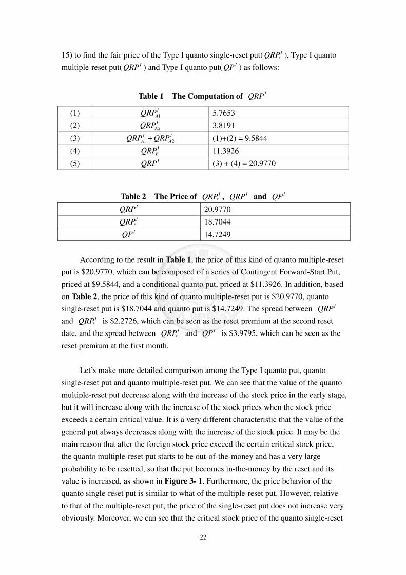
Table 1 The Computation of IQRP
(1) 1
I
AQRP 5.7653
(2) 2
I
AQRP 3.8191
(3) 1 2
I I
A AQRP QRP+ (1)+(2) = 9.5844
(4) I
BQRP 11.3926
(5) IQRP (3) + (4) = 20.9770
Table 2 The Price of *
IQRP , IQRP and IQP IQRP 20.9770
*
IQRP 18.7044 IQP 14.7249
According to the result in Table 1, the price of this kind of quanto multiple-reset
put is $20.9770, which can be composed of a series of Contingent Forward-Start Put,
priced at $9.5844, and a conditional quanto put, priced at $11.3926. In addition, based
on Table 2, the price of this kind of quanto multiple-reset put is $20.9770, quanto
single-reset put is $18.7044 and quanto put is $14.7249. The spread between IQRP
and *
IQRP is $2.2726, which can be seen as the reset premium at the second reset
date, and the spread between *
IQRP and IQP is $3.9795, which can be seen as the
reset premium at the first month.
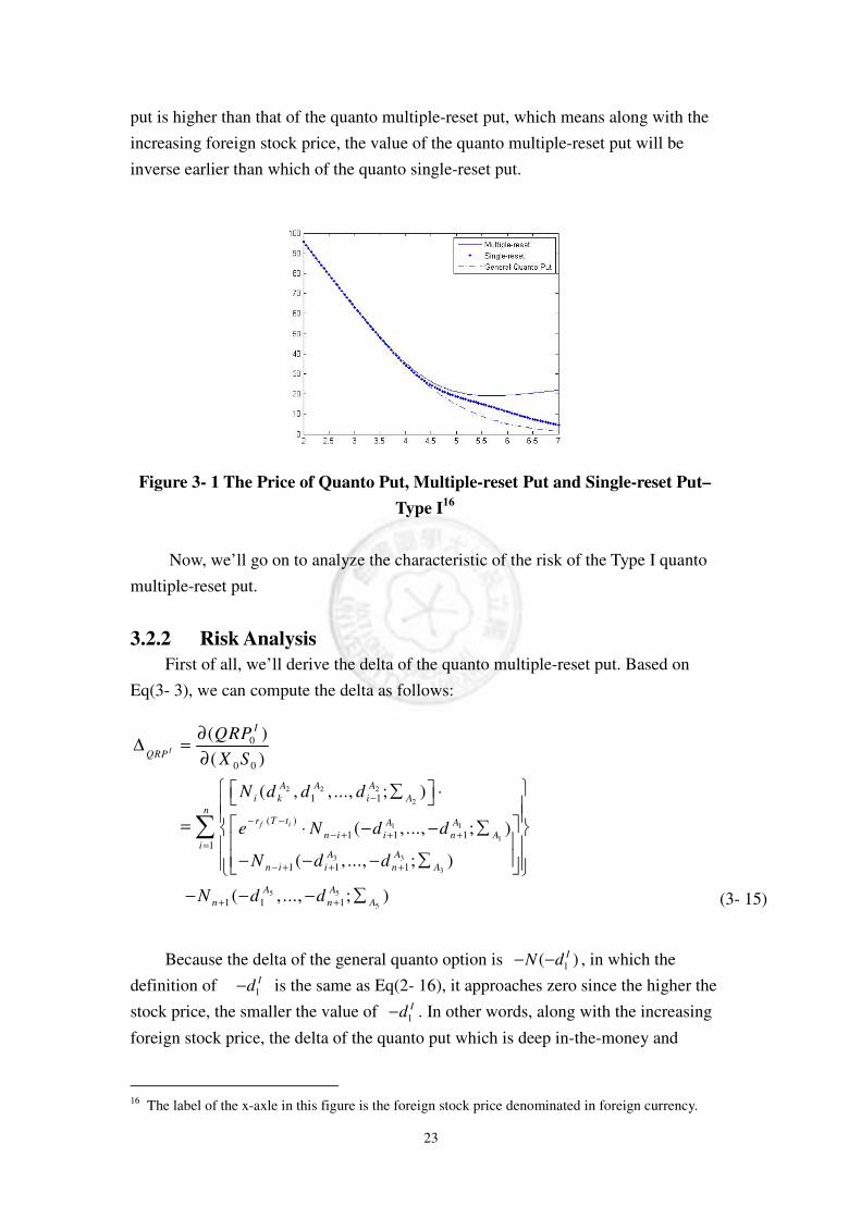
Let’s make more detailed comparison among the Type I quanto put, quanto
single-reset put and quanto multiple-reset put. We can see that the value of the quanto
multiple-reset put decrease along with the increase of the stock price in the early stage,
but it will increase along with the increase of the stock prices when the stock price
exceeds a certain critical value. It is a very different characteristic that the value of the
general put always decreases along with the increase of the stock price. It may be the
main reason that after the foreign stock price exceed the certain critical stock price,
the quanto multiple-reset put starts to be out-of-the-money and has a very large
probability to be resetted, so that the put becomes in-the-money by the reset and its
value is increased, as shown in Figure 3- 1. Furthermore, the price behavior of the
quanto single-reset put is similar to what of the multiple-reset put. However, relative
to that of the multiple-reset put, the price of the single-reset put does not increase very
obviously. Moreover, we can see that the critical stock price of the quanto single-reset
23
put is higher than that of the quanto multiple-reset put, which means along with the
increasing foreign stock price, the value of the quanto multiple-reset put will be
inverse earlier than which of the quanto single-reset put.
Figure 3- 1 The Price of Quanto Put, Multiple-reset Put and Single-reset Put–
Type I16
Now, we’ll go on to analyze the characteristic of the risk of the Type I quanto
multiple-reset put.
3.2.2 Risk Analysis
First of all, we’ll derive the delta of the quanto multiple-reset put. Based on
Eq(3- 3), we can compute the delta as follows:
Because the delta of the general quanto option is 1( )IN d− − , in which the
definition of 1
Id− is the same as Eq(2- 16), it approaches zero since the higher the
stock price, the smaller the value of 1
Id− . In other words, along with the increasing
foreign stock price, the delta of the quanto put which is deep in-the-money and
16 The label of the x-axle in this figure is the foreign stock price denominated in foreign currency.
2 2 2
2
1 1
1
3 3
3
5 5
5
0
0 0
1 1
( )
1 1 11
1 1 1
1 1 1
( )
( )
( , , ..., ; )
( , ..., ; )
( , ..., ; )
( , ..., ; )
I
f i
I
QRP
A A A
i k i A
nr T t A A
n i i n Ai
A A
n i i n A
A A
n n A
QRP
X S
N d d d
e N d d
N d d
N d d
−
− −
− + + +=
− + + +
+ +
∂∆ =
∂
∑ ⋅ = ⋅ − − ∑ − − − ∑
− − − ∑
∑
(3- 15)
24
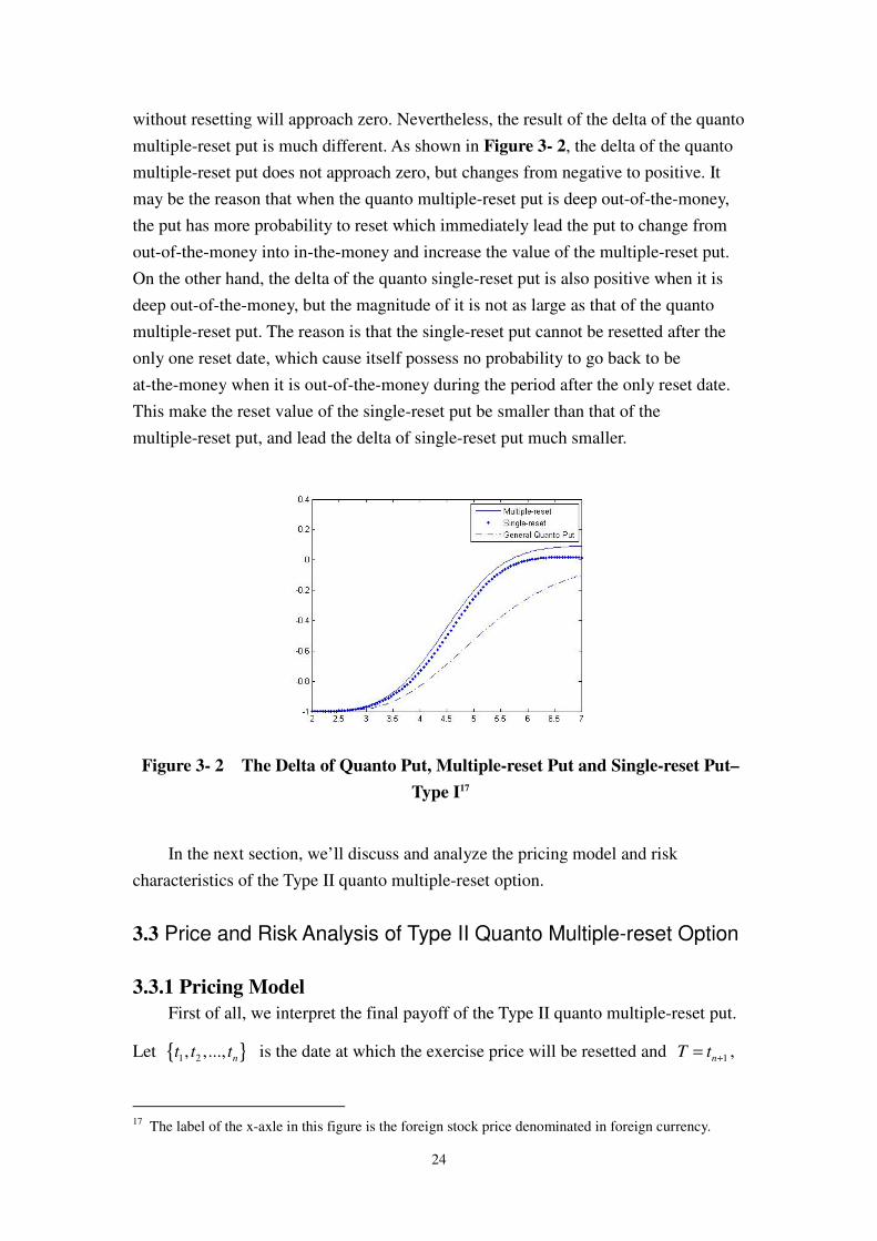
without resetting will approach zero. Nevertheless, the result of the delta of the quanto
multiple-reset put is much different. As shown in Figure 3- 2, the delta of the quanto
multiple-reset put does not approach zero, but changes from negative to positive. It
may be the reason that when the quanto multiple-reset put is deep out-of-the-money,
the put has more probability to reset which immediately lead the put to change from
out-of-the-money into in-the-money and increase the value of the multiple-reset put.
On the other hand, the delta of the quanto single-reset put is also positive when it is
deep out-of-the-money, but the magnitude of it is not as large as that of the quanto
multiple-reset put. The reason is that the single-reset put cannot be resetted after the
only one reset date, which cause itself possess no probability to go back to be
at-the-money when it is out-of-the-money during the period after the only reset date.
This make the reset value of the single-reset put be smaller than that of the
multiple-reset put, and lead the delta of single-reset put much smaller.
Figure 3- 2 The Delta of Quanto Put, Multiple-reset Put and Single-reset Put–
Type I17
In the next section, we’ll discuss and analyze the pricing model and risk
characteristics of the Type II quanto multiple-reset option.
3.3 Price and Risk Analysis of Type II Quanto Multiple-reset Option
3.3.1 Pricing Model
First of all, we interpret the final payoff of the Type II quanto multiple-reset put.
Let { }1 2, ,..., nt t t is the date at which the exercise price will be resetted and 1nT t += ,
17 The label of the x-axle in this figure is the foreign stock price denominated in foreign currency.
25
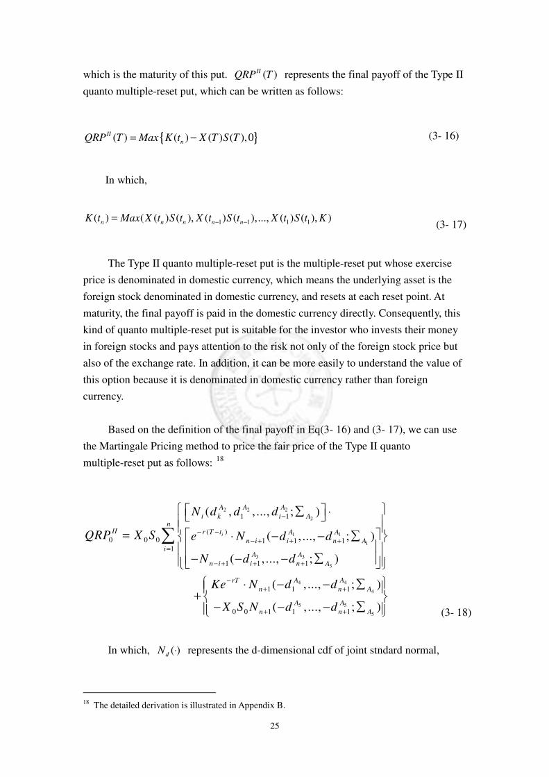
which is the maturity of this put. ( )IIQRP T represents the final payoff of the Type II
quanto multiple-reset put, which can be written as follows:
In which,
The Type II quanto multiple-reset put is the multiple-reset put whose exercise
price is denominated in domestic currency, which means the underlying asset is the
foreign stock denominated in domestic currency, and resets at each reset point. At
maturity, the final payoff is paid in the domestic currency directly. Consequently, this
kind of quanto multiple-reset put is suitable for the investor who invests their money
in foreign stocks and pays attention to the risk not only of the foreign stock price but
also of the exchange rate. In addition, it can be more easily to understand the value of
this option because it is denominated in domestic currency rather than foreign
currency.
Based on the definition of the final payoff in Eq(3- 16) and (3- 17), we can use
the Martingale Pricing method to price the fair price of the Type II quanto
multiple-reset put as follows: 18
In which, ( )dN ⋅ represents the d-dimensional cdf of joint stndard normal,
18 The detailed derivation is illustrated in Appendix B.
{ }( ) ( ) ( ) ( ),0II
nQRP T Max K t X T S T= − (3- 16)
1 1 1 1( ) ( ( ) ( ), ( ) ( ),..., ( ) ( ), )n n n n nK t Max X t S t X t S t X t S t K− −= (3- 17)
2 2 2
2
1 1
1
3 3
3
4 4
4
5
1 1
( )0 0 0 1 1 1
1
1 1 1
1 1 1
0 0 1 1
( , , ..., ; )
( , ..., ; )
( , ..., ; )
( , ..., ; )
( , ...,
i
A A A
i k i An
II r T t A A
n i i n Ai
A A
n i i n A
A ArT
n n A
A
n
N d d d
QRP X S e N d d
N d d
Ke N d d
X S N d d
−
− −
− + + +=
− + + +
−+ +
+
∑ ⋅ = ⋅ − − ∑
− − − ∑
⋅ − − ∑+
− − −
∑
5
51; )A
n A+
∑
(3- 18)
26
iA∑ represents each of the correlation matrix in the d-dimensional cdf of joint
stndard normal. All the parameters in Eq(3- 18) are illustrated as follows:
1
2
( )( )2 ,
sxj i
A
j
SX j i
r t t
d i jt t
σ
σ
− −= <
− (3- 19)
2
2
0 0ln( ) ( )2SX
iA
K
SX i
X Sr t
Kdt
σ
σ
+ += (3- 20)
2
2
( )( )2 ,
SXi h
A
h
SX i h
r t t
d h it t
σ
σ
+ −= <
− (3- 21)
3
2
( )( )2 ,
sxj i
A
j
sx j i
r t t
d i jt t
σ
σ
+ −= <
− (3- 22)
4
2
0 0ln( ) ( )2sx
jA
j
sx j
X Sr t
Kdt
σ
σ
+ −= (3- 23)
5
2
0 0ln( ) ( )2sx
jA
j
sx j
X Sr t
Kdt
σ
σ
+ += (3- 24)
The definition of sxσ is the same as Eq(2- 4), and 1A∑ ,
2A∑ ,3A∑ ,
4A∑
and 5A∑ is the same as Eq(3- 10)~(3- 12).
If we let 1n = , the reset date be 0t and the maturity of the put be 1nT t += and
put them back into Eq(3- 18), we’ll have the pricing formula of the Type II quanto
single-reset put as follows:

27
We can compare the Eq(3- 25) with the result in Jiang(2004), and we can find
the two pricing formulas are consistent.
On the other hand, we can rewrite Eq(3- 18) as follows:
Similar to the prior section, based on Eq(3- 14), we can find that the Type II
quanto multiple-reset put( IIQRP ) is composed of the n units of Contingent
Forward-Start Put19 and a conditional quanto put20. Similarly, in order to more easily
explain how the 2 kinds of options affect the Type II quanto multiple-reset put, we
take the same numerical example to illustrate it. In this example, because of the
exercise price denominated in domestic currency, we assume the initial exercise price
19 That is
II
AiQRP .
20 That is II
BQRP .
0 32 1
4 4
4
5 5
5
( )
0 0 0 2 2
2 1 2
0 0 2 1 2
( ) ( ) ( )
( , ; )
( , ; )
r T t AA AII
k
A ArT
A
A A
A
QRP X S N d e N d N d
Ke N d d
X S N d d
− −
−
= ⋅ ⋅ − − −
⋅ − − ∑ +
− ⋅ − − ∑
(3- 25)
2 2 2
2
1 1
1
3 32 2 2
2 3
( )
0 1 1
1 1 10 0
0 1 1 1 1 1
( , ,..., ; )
( ,..., ; )
( , ,..., ; ) ( ,..., ; )
i
IIAi
r T t A A A
i k i A
A AIIn i i n A
A AA A A
i k i A n i i n A
QRP
S e N d d d
N d dQRP X
S N d d d N d d
− −
−
− + + +
− − + + +
∑ ⋅ −
− − ∑ = ∑ ⋅ − − ∑ 14444444444442444444444 3
( ) { }{ }
4 4
4
5 5
5
1 1
1
1 1 1
0 0 1 1 1
1
{ ( ) ( ) ( ) ( ),..., ( ) ( ), }
( ,..., ; )
( ,..., ; )
( ( ) ( ) ( ) ( )
IIB
i i n n
n
i
A ArT
n n A
A A
n n A
QRP
nII II
Ai B
i
rT Q
i i X t S t Max X t S t X t S t K
Q
Ke N d d
X S N d d
QRP QRP
e E X t S t X T S T I
=
−+ +
+ +
=
+−
=
⋅ − − ∑ +
− ⋅ − − ∑
= +
= − ⋅
∑
∑
444
144444424444443
( ) { }{ }1 1
1
{ ( ) ( ),..., ( ) ( ), }( ( ) ( )
IIAi
n n
IIB
n
i
RP
rT Q
K Max X t S t X t S t K
QRP
e E K X T S T I
=
+−
=+ − ⋅
∑14444444444444244444444444443
14444444444244444444443
(3- 26)
28
is 05 162.5K X= × = . Substitute all of the parameters we assume into Eq(3- 13),
Eq(3- 3)~(3- 12) and Eq(2- 15) and we’ll find the fair price of the Type II quanto
single-reset put( *
IIQRP ), Type II quanto multiple-reset put( IIQRP ) and Type II quanto
put( IIQP ) as follows:
Table 3 The Computation of IIQRP
(1) 1
II
AQRP 8.9683
(2) 2
II
AQRP 5.8968
(3) 1 2
II II
A AQRP QRP+ (1)+(2) = 14.8651
(4) II
BQRP 17.7289
(5) IIQRP (3) + (4) = 32.5940
Table 4 The Price of *
IIQRP , IIQRP and IIQP IIQRP 32.5940
*
IIQRP 29.0463 IIQP 20.4631
According to the result in Table 3, the price of this kind of quanto multiple-reset
put is $32.5490, which can be composed of a series of Contingent Forward-Start Put,
priced at $14.8651, and a conditional quanto put, priced at $17.7289. In addition,
based on Table 4, the price of this kind of quanto multiple-reset put is $32.5740,
quanto single-reset put is $29.0463 and quanto put is $20.4631. The spread between IIQRP and *
IIQRP is $3.5477, which can be seen as the reset premium at the second
reset date, and the spread between *
IIQRP and IIQP is $8.5832, which can be seen
as the reset premium at the first month.
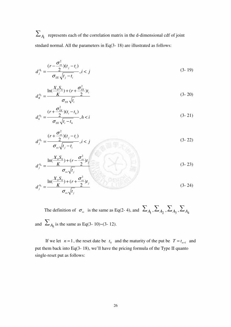
Similar to the prior section, let’s make more detailed comparison among the
Type II quanto put, quanto single-reset put and quanto multiple-reset put. Also, as
shown in Figure 3- 3, we can see that the value of the quanto multiple-reset put
decrease along with the increase of the stock price in the early stage, but it will
increase along with the increase of the stock prices when the stock price exceeds a
certain critical value. It is a very different characteristic that the value of the general
put always decreases along with the increase of the stock price. The main reason is the
same as which we explain in the prior section, so we don’t describe it again.
29
Figure 3- 3 The Price of Quanto Put, Multiple-reset Put and Single-reset Put–
Type II21
Now, we’ll go on to analyze the characteristic of the risk of the Type II quanto
multiple-reset put.
3.3.2 Risk Analysis
Similarly, we’ll derive the delta of the quanto multiple-reset put. Based on Eq(3-
18), we can compute the delta as follows:
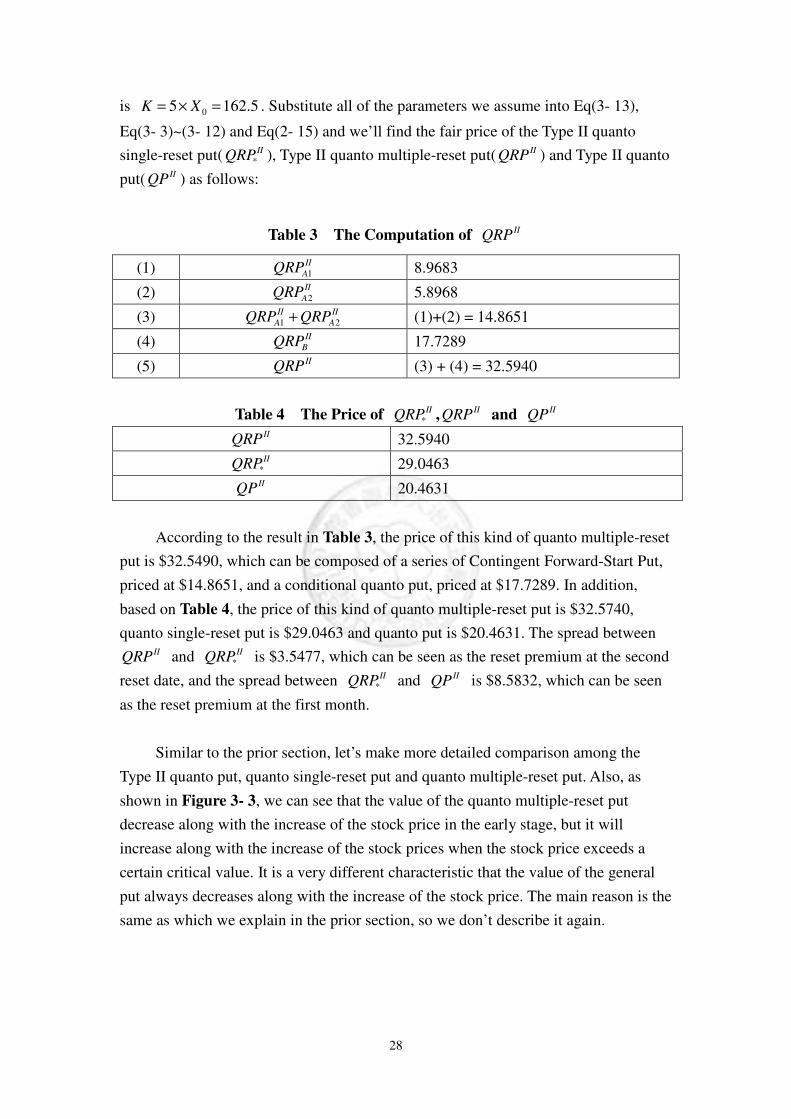
The relationship among the delta of Type II quanto put, Type II quanto
single-reset put and Type II multiple-reset put is shown in Figure 3- 4.
21 The label of the x-axle in this figure is the foreign stock price denominated in domestic currency.
2 2 2
2
1 1
1
3 3
3
5 5
5
0
0 0
1 1
( )
1 1 11
1 1 1
1 1 1
( )
( )
( , , ..., ; )
( , ..., ; )
( , ..., ; )
( , ..., ; )
II
i
II
QRP
A A A
i k i An
r T t A A
n i i n Ai
A A
n i i n A
A A
n n A
QRP
X S
N d d d
e N d d
N d d
N d d
−
− −
− + + +=
− + + +
+ +
∂∆ =
∂
∑ ⋅ = ⋅ − − ∑
− − − ∑
− − − ∑
∑
(3- 27)
30
Figure 3- 4 The Delta of Quanto Put, Multiple-reset Put and Single-reset Put–
Type II22
We can see that the delta of the quanto multiple-reset put does not approach zero
when it is deep out-of-the-money, but changes from negative to positive. On the other
hand, the delta of the quanto single-reset put is also positive when it is deep
out-of-the-money, but the magnitude of it is not as large as that of the quanto
multiple-reset put. The main reason is the same as which we explain in the prior
section, so we don’t describe it again.
In the next section, we’ll discuss and analyze the pricing model and risk
characteristics of the Type III quanto multiple-reset option.
3.4 Price and Risk Analysis of Type III Quanto Multiple-reset Option
3.4.1 Pricing Model
Equally, we interpret the final payoff of the Type III quanto multiple-reset put.
Let { }1 2, ,..., nt t t is the date at which the exercise price will be resetted and 1nT t += ,
which is the maturity of this put. ( )IIIQRP T represents the final payoff of the Type
III quanto multiple-reset put, which can be written as follows:
22 The label of the x-axle in this figure is the foreign stock price denominated in domestic currency.
{ }( ) ( ) ( ),0III
nQRP T Max K t S Tχ= ⋅ − (3- 28)
31
In which, χ represents the fixed exchange rate decided initially and
The Type III quanto multiple-reset put is the multiple-reset put whose exercise
price is resetted at each reset point. At maturity, the final payoff is liquidated by
foreign currency and transferred into the domestic value by the fixed exchange rate
decided at the beginning. Consequently, this kind of quanto multiple-reset put is equal
to a multiple-reset put whose underlying asset is the foreign stock and transferred into
domestic value by a fixed rate. By this kind of quanto multiple-reset put, we can not
only protect the put value against the decline of foreign stock price, which cause the
value of the put decrease, but also capture the capital gain of the rise of the foreign
stock price. Therefore, the Type III quanto multiple-reset put is suitable for the
investor who invests their money in foreign stocks and pays attention to the risk not
only of the foreign stock price but also of the exchange rate.
Based on the definition of the final payoff in Eq(3- 28) and (3- 29), we can use
the Martingale Pricing method to price the fair price of the Type III quanto
multiple-reset put as follows23:
In which, ( )dN ⋅ represents the d-dimensional cdf of joint stndard normal,
iA∑ represents each of the correlation matrix in the d-dimensional cdf of joint
stndard normal. All the parameters in Eq(3- 30) are illustrated as follows:
23 The detailed derivation is illustrated in Appendix C.
1 1( ) ( ( ), ( ),..., ( ), )n n nK t Max S t S t S t K−= (3- 29)
, 2 2 2
2
1 1
1
3 3
3
4 4
4
( )
1 1
( )0 1 1 1
1
0 1 1 1
1 1 1
0
( , , ..., ; )
( , ..., ; )
( , ..., ; )
( , ..., ; )
f S X S X i
i
r r t A A A
i k i An
r T t A A
n i i n Ai
III A A
n i i n A
A ArT
n n A
e N d d d
S e N d d
QRP N d d
Ke N d d
S
ρ σ σ
χ
− − +
−
− −
− + + +=
− + + +
−+ +
∑ ⋅ ⋅ − − ∑
= − − − ∑
⋅ − − ∑+
−
∑
, 5 5
5
( )
1 1 1( , ..., ; )f S X S Xr r T A A
n n Ae N d dρ σ σ− − +
+ +
− − ∑
(3- 30)
32
1
2
,( )( )2 ,
sf S X s X j i
A
j
s j i
r t t
d i jt t
σρ σ σ
σ
− − −= <
− (3- 31)
2
2
0,ln( ) ( )
2s
f S X s X iA
K
s i
Sr t
Kdt
σρ σ σ
σ
+ − += (3- 32)
2
2
,( )( )2 ,
sf S X s X i h
A
h
s i h
r t t
d h it t
σρ σ σ
σ
− + −= <
−
(3- 33)
3
2
,( )( )2 ,
sf S X s X j i
A
j
s j i
r t t
d i jt t
σρ σ σ
σ
− + −= <
− (3- 34)
4
2
0,ln( ) ( )
2s
f S X s X jA
j
s j
Sr t
Kdt
σρ σ σ
σ
+ − −= (3- 35)
5
2
0,ln( ) ( )
2s
f S X s X jA
j
s j
Sr t
Kdt
σρ σ σ
σ
+ − += (3- 36)
The definitions of 1A∑ ,
2A∑ ,3A∑ ,
4A∑ and5A∑ are the same as Eq(3-
10)~(3- 12).
If we let 1n = , the reset date be 0t and the maturity of the put be 1nT t += and
put them back into Eq(3- 30), we’ll have the pricing formula of the Type III quanto
single-reset put as follows:
We can compare the Eq(3- 37) with the result in Jiang(2004), and we can find
, 0 2
0 31
4 4
4
, 5 5
5
( )
0
( )
2 2
0 2 1 2
( )
0 2 1 2
( )
( ) ( )
( , ; )
( , ; )
f S X S X
f S X S X i
r r t A
k
r T t AA
A AIII rT
A
r r t A A
A
S e N d
e N d N d
QRP Ke N d d
S e N d d
ρ σ σ
ρ σ σ
χ
− − +
− −
−
− − +
⋅ ⋅ − − −
= ⋅ + ⋅ − − ∑
− ⋅ − − ∑
(3- 37)
33
the two pricing formulas are consistent.
On the other hand, we can rewrite Eq(3- 30) as follows:
Similar to the prior section, based on Eq(3- 38), we can find that the Type III
quanto multiple-reset put( IIIQRP ) is composed of the n units of Contingent
Forward-Start Put24 and a conditional quanto put25. Similarly, in order to more easily
explain how the 2 kinds of options affect the Type III quanto multiple-reset put, we
take the same numerical example to illustrate it. In this example, we assume the fixed
rate decided at the beginning is 0 32.5Xχ = = . Substitute all of the parameters we
assume into Eq(3- 37), Eq(3- 30)~(3- 36) and Eq(2- 24) and we’ll find the fair price
of the Type III quanto single-reset put( *
IIIQRP ), Type III quanto multiple-reset
put( IIIQRP ) and Type III quanto put( IIIQP ) as follows:
Table 5 The Computation of IIIQRP
(1) 1
III
ARP26 0.1779
24 That is
III
AiRP .
25 That is III
BRP .
26 The values of 1
III
ARP , 2
III
ARP and III
BRP are denominated in foreign currency.
, 2 2 2
2
1 1
1
3 3
3
( )
1 1
( )0 1 1 1
1
1 1 1
0
( , , ..., ; )
( , ..., ; )
( , ..., ; )
f S X S X i
i
IIIAi
r r t A A A
i k i An
r T t A A
n i i n Ai
A A
n i i n AIII
RP
rT
n
e N d d d
S e N d d
N d d
QRP
Ke N
ρ σ σ
χ
− − +
−
− −
− + + +=
− + + +
−
∑ ⋅ ⋅ − − ∑ − − − ∑
=
⋅+
∑
144444444424444444443
( )
4 4
4
, 5 5
5
B
1 1 1
( )
0 1 1 1
1
{ ( ) ( ),
( , ..., ; )
( , ..., ; )
( ( ) ( )
f S X S X
III
i n
A A
n A
r r T A A
n n A
RP
nII II
Ai B
i
rT Q
i S t Max S t
d d
S e N d d
RP RP
e E S t S T I
ρ σ σ
χ
χ
+ +
− − +
+ +
=
+−
=
− − ∑
− − − ∑
= ⋅ +
− ⋅
=
∑
144444444424444444443
{ }{ }
( ) { }{ }
1
1
..., ( ), }1
{ ( ),..., ( ), }( ( )
IIIAi
n
IIIB
n
S t K
i
RP
rT Q
K Max S t S t K
RP
e E K S T I
=
+−
=
+ − ⋅
∑144444444424444444443
1444444442444444443
(3- 38)
34
(2) 2
III
ARP 0.1121
(3) 1 2
III III
A ARP RP+ (1) + (2) = 0.2900
(4) III
BRP 0.3942
(5) IIIQRP [ ](3) (4)χ ⋅ + = 22.2356
Table 6 The Price of *
IIIQRP , IIIQRP and IIIQP IIIQRP 22.2356
*
IIIQRP 19.8926 IIIQP 15.0265
According to the result in Table 5, the price of this kind of quanto multiple-reset
put is $22.2356, which can be composed of a series of Contingent Forward-Start Put,
priced at 0.2900, which is denominated in foreign currency, and a conditional quanto
put, priced at 0.3942, which is also denominated in foreign currency. In addition,
based on Table 6, the price of this kind of quanto multiple-reset put is $22.2356,
quanto single-reset put is $19.8926 and quanto put is $15.0625. The spread between IIIQRP and *
IIIQRP is $2.1523, which can be seen as the reset premium at the
second reset date, and the spread between *
IIIQRP and IIIQP is $4.8701, which can
be seen as the reset premium at the first month.
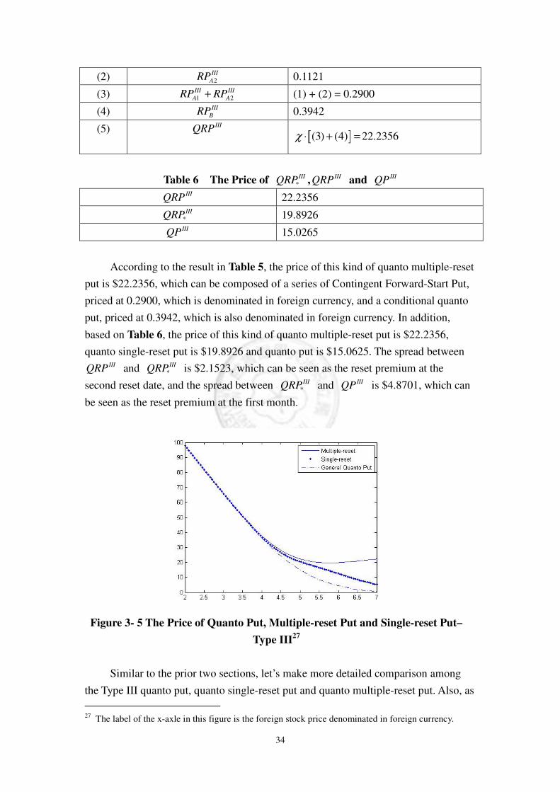
Figure 3- 5 The Price of Quanto Put, Multiple-reset Put and Single-reset Put–
Type III27
Similar to the prior two sections, let’s make more detailed comparison among
the Type III quanto put, quanto single-reset put and quanto multiple-reset put. Also, as
27 The label of the x-axle in this figure is the foreign stock price denominated in foreign currency.
35
shown in Figure 3- 5, we can see that the value of the quanto multiple-reset put
decrease along with the increase of the stock price in the early stage, but it will
increase along with the increase of the stock prices when the stock price exceeds a
certain critical value. It is a very different characteristic that the value of the general
put always decreases along with the increase of the stock price. The main reason is the
same as which we explain in the prior section, so we don’t describe it again.
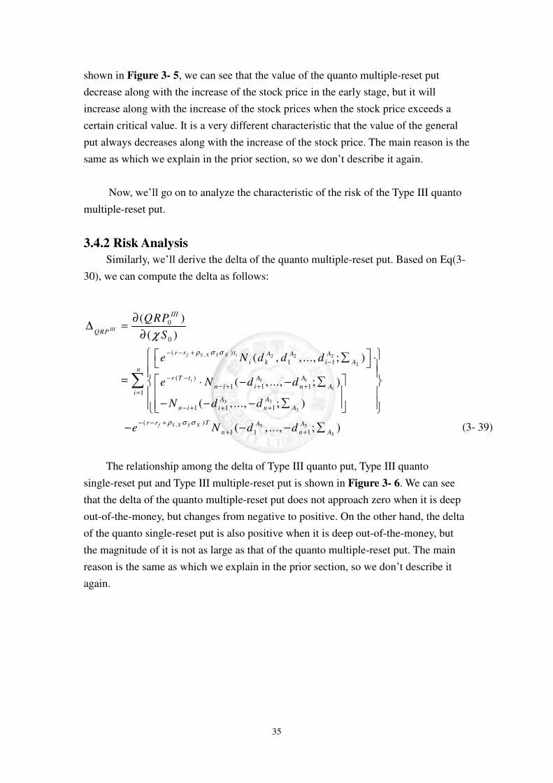
Now, we’ll go on to analyze the characteristic of the risk of the Type III quanto
multiple-reset put.
3.4.2 Risk Analysis
Similarly, we’ll derive the delta of the quanto multiple-reset put. Based on Eq(3-
30), we can compute the delta as follows:
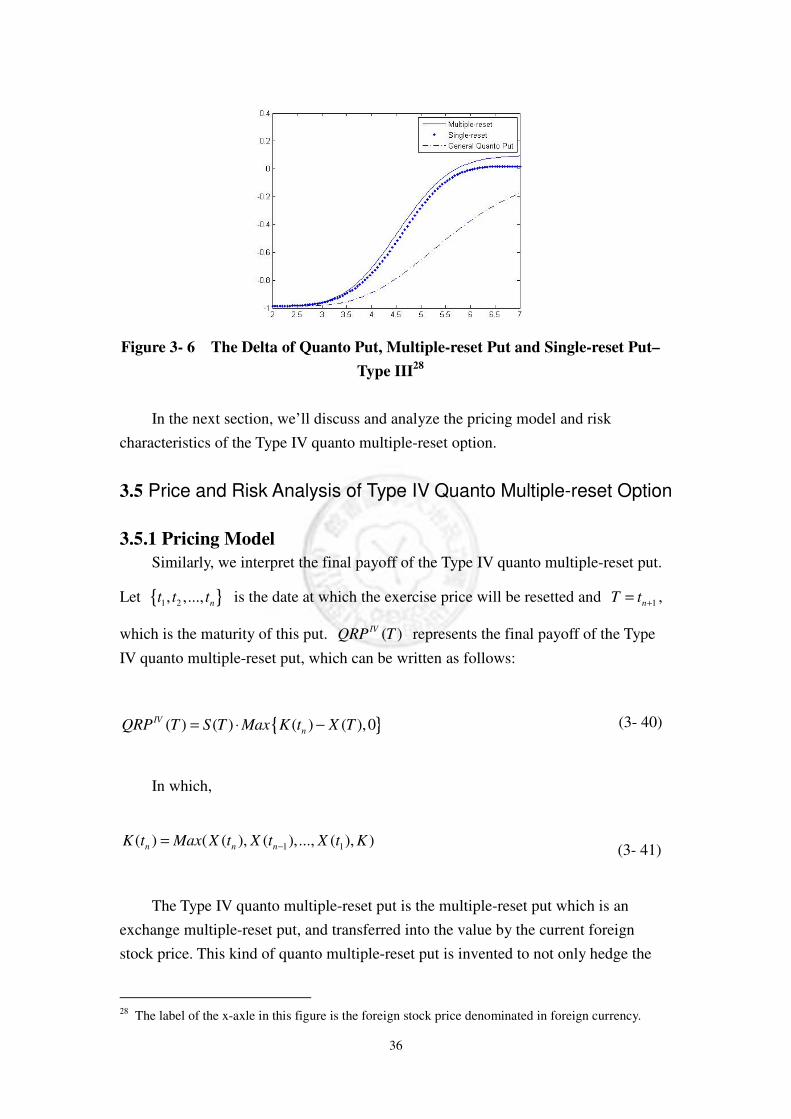
The relationship among the delta of Type III quanto put, Type III quanto
single-reset put and Type III multiple-reset put is shown in Figure 3- 6. We can see
that the delta of the quanto multiple-reset put does not approach zero when it is deep
out-of-the-money, but changes from negative to positive. On the other hand, the delta
of the quanto single-reset put is also positive when it is deep out-of-the-money, but
the magnitude of it is not as large as that of the quanto multiple-reset put. The main
reason is the same as which we explain in the prior section, so we don’t describe it
again.
, 2 2 2
2
1 1
1
3 3
3
,
0
0
( )
1 1
( )
1 1 11
1 1 1
( )
1
( )
( )
( , , ..., ; )
( , ..., ; )
( , ..., ; )
III
f S X S X i
i
f S X S X
III
QRP
r r t A A A
i k i An
r T t A A
n i i n Ai
A A
n i i n A
r r T
n
QRP
S
e N d d d
e N d d
N d d
e N
ρ σ σ
ρ σ σ
χ
− − +
−
− −
− + + +=
− + + +
− − +
+
∂∆ =
∂
∑ ⋅
= ⋅ − − ∑ − − − ∑
−
∑
5 5
51 1( , ..., ; )A A
n Ad d +− − ∑
(3- 39)
36
Figure 3- 6 The Delta of Quanto Put, Multiple-reset Put and Single-reset Put–
Type III28
In the next section, we’ll discuss and analyze the pricing model and risk
characteristics of the Type IV quanto multiple-reset option.
3.5 Price and Risk Analysis of Type IV Quanto Multiple-reset Option
3.5.1 Pricing Model
Similarly, we interpret the final payoff of the Type IV quanto multiple-reset put.
Let { }1 2, ,..., nt t t is the date at which the exercise price will be resetted and 1nT t += ,
which is the maturity of this put. ( )IVQRP T represents the final payoff of the Type
IV quanto multiple-reset put, which can be written as follows:
In which,
The Type IV quanto multiple-reset put is the multiple-reset put which is an
exchange multiple-reset put, and transferred into the value by the current foreign
stock price. This kind of quanto multiple-reset put is invented to not only hedge the
28 The label of the x-axle in this figure is the foreign stock price denominated in foreign currency.
{ }( ) ( ) ( ) ( ),0IV
nQRP T S T Max K t X T= ⋅ − (3- 40)
1 1( ) ( ( ), ( ),..., ( ), )n n nK t Max X t X t X t K−= (3- 41)
37
downward exchange risk but also allow the investor to capture the capital gain from
the appreciation of the exchange rate. Consequently, it is suitable for the investor who
invests their money in foreign stocks and pays more attention to the risk of the
exchange rate than the foreign stock price.
Based on the definition of the final payoff in Eq(3- 40) and (3- 41), we can use
the Martingale Pricing method to price the fair price of the Type IV quanto
multiple-reset put as follows29:
Similarly, in which, ( )dN ⋅ represents the d-dimensional cdf of joint stndard
normal, iA∑ represents each of the correlation matrix in the d-dimensional cdf of
joint stndard normal. All the parameters in Eq(3- 42) are illustrated as follows:
1
2
,( )( )2 ,
Xf S X s X j i
A
j
X j i
r r t t
d i jt t
σρ σ σ
σ
− − + −= <
− (3- 43)
2
2
0,ln( ) ( )
2X
f S X S X iA
K
X i
Xr r t
Kdt
σρ σ σ
σ
+ − + += (3- 44)
2
2
,( )( )2 ,
Xf S X S X i h
A
h
X i h
r r t t
d h it t
σρ σ σ
σ
− + + −= <
− (3- 45)
3
2
,( )( )2 ,
Xf S X S X j i
A
j
X j i
r r t t
d i jt t
σρ σ σ
σ
− + + −= <
− (3- 46)
29 The detailed derivation is illustrated in Appendix D.
2 2 2
2
, 1 1
1
3 3
3
, 4
1 1
( )( )0 0 0 1 1 1
1
1 1 1
( )
1 1
0
( , ,..., ; )
( ,..., ; )
( ,..., ; )
( ,...,
f S X S X i
f S X S X
A A A
i k i A
nIV r r T t A A
n i i n Ai
A A
n i i n A
r r T A
n n
N d d d
QRP S X e N d d
N d d
Ke N d dS
ρ σ σ
ρ σ σ
−
− − + −
− + + +=
− + + +
− − +
+ +
∑ ⋅ = ⋅ − − ∑ − − − ∑
⋅ − −+
∑
4
4
5 5
5
1
0 1 1 1
; )
( ,..., ; )
A
A
A A
n n AX N d d+ +
∑
− − − ∑
(3- 42)
38
4
2
0,ln( ) ( )
2X
f S X S X jA
j
X j
Xr r t
Kdt
σρ σ σ
σ
+ − − += (3- 47)
5
2
0,ln( ) ( )
2X
f S X S X jA
j
X j
Xr r t
Kdt
σρ σ σ
σ
+ − + += (3- 48)
The definitions of 1A∑ ,
2A∑ ,3A∑ ,
4A∑ and5A∑ are the same as Eq(3-
10)~(3- 12).
If we let 1n = , the reset date be 0t and the maturity of the put be 1nT t += and
put them back into Eq(3- 42), we’ll have the pricing formula of the Type IV quanto
single-reset put as follows:
We can compare the Eq(3- 49) with the result in Jiang(2004), and we can find
the two pricing formulas are consistent.
On the other hand, we can rewrite Eq(3- 49) as follows:
, 0 32 1
, 4 4
4
5 5
5
( )( )
0 0 0 2 2
( )
2 1 2
0
0 2 1 2
( ) ( ) ( )
( , ; )
( , ; )
f S X S X
f S X S X
r r T t AA AIV
k
r r T A A
A
A A
A
QRP S X N d e N d N d
Ke N d dS
X N d d
ρ σ σ
ρ σ σ
− − + −
− − +
= ⋅ ⋅ − − −
⋅ − − ∑ +
− − − ∑
(3- 49)
39
Based on Eq(3- 50), we can find that the Type IV quanto multiple-reset
put( IVQRP ) is composed of the n units of Contingent Forward-Start Put30 and a
conditional quanto put31. Similarly, in order to more easily explain how the 2 kinds of
options affect the Type IV quanto multiple-reset put, we take the same numerical
example to illustrate it. In this example, because K is the exercise price of the
exchange rate put, we assume it is 0 32.5K X= = . Substitute all of the parameters we
assume into Eq(3- 49), Eq(3- 42)~(3- 48) and Eq(2- 28) and we’ll find the fair price
of the Type IV quanto single-reset put( *
IVQRP ), Type IV quanto multiple-reset
put( IVQRP ) and Type IV quanto put( IVQP ) as follows:
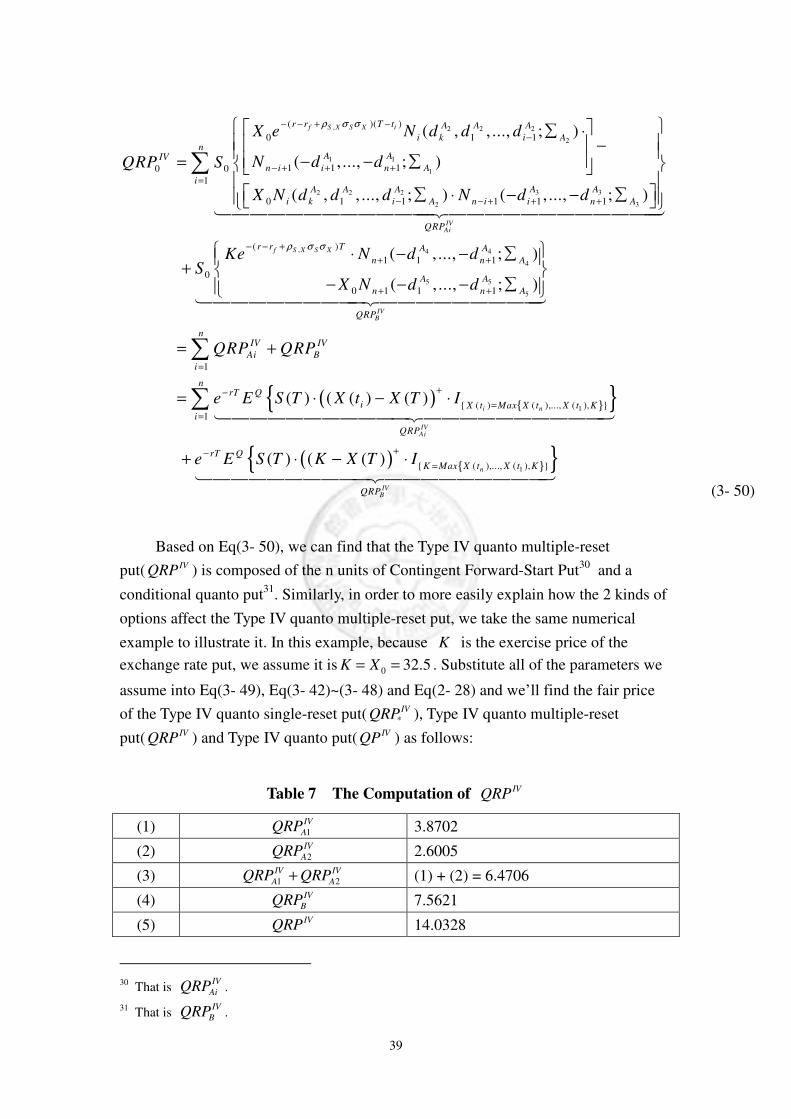
Table 7 The Computation of IVQRP
(1) 1
IV
AQRP 3.8702
(2) 2
IV
AQRP 2.6005
(3) 1 2
IV IV
A AQRP QRP+ (1) + (2) = 6.4706
(4) IV
BQRP 7.5621
(5) IVQRP 14.0328
30 That is
IV
AiQRP .
31 That is IV
BQRP .
, 2 2 2
2
1 1
1
3 32 2 2
2 3
( )( )
0 1 1
1 1 10 0
0 1 1 1 1 1
( , , ..., ; )
( , ..., ; )
( , , ..., ; ) ( , ..., ; )
f S X S X i
IVAi
r r T t A A A
i k i A
A AIV
n i i n A
A AA A A
i k i A n i i n A
QRP
X e N d d d
N d dQRP S
X N d d d N d d
ρ σ σ− − + −
−
− + + +
− − + + +
∑ ⋅ − − − ∑= ∑ ⋅ − − ∑ 144444444 2
( )
, 4 4
4
5 5
5
1
( )
1 1 1
0
0 1 1 1
1
{ ( ) ( )
( , ..., ; )
( , ..., ; )
( ) ( ( ) ( )
f S X S X
IVB
i n
n
i
r r T A A
n n A
A A
n n A
QRP
nIV IV
Ai B
i
rT Q
i X t Max X t
Ke N d dS
X N d d
QRP QRP
e E S T X t X T I
ρ σ σ
=
− − +
+ +
+ +
=
+−
=
⋅ − − ∑ +
− − − ∑
= +
= ⋅ − ⋅
∑
∑
4444 4444444444443
144444444424444444443
{ }{ }
( ) { }{ }
1
1
,..., ( ), }1
{ ( ),..., ( ), }( ) ( ( )
IVAi
n
IVB
n
X t K
i
QRP
rT Q
K Max X t X t K
QRP
e E S T K X T I
=
+−
=+ ⋅ − ⋅
∑14444444444244444444443
144444444424444444443
(3- 50)
40
Table 8 The Price of *
IVQRP , IVQRP and IVQP IVQRP 14.0328
*
IVQRP 12.4890 IVQP 10.1264
According to the result in Table 7, the price of this kind of quanto multiple-reset
put is $14.0328, which can be composed of a series of Contingent Forward-Start Put,
priced at $6.4706, which is denominated in foreign currency, and a conditional quanto
put, priced at $7.5621, which is also denominated in foreign currency. In addition,
based on Table 8, the price of this kind of quanto multiple-reset put is $14.0328,
quanto single-reset put is $12.4890 and quanto put is $10.1264. The spread between IIIQRP and *
IIIQRP is $2.5438, which can be seen as the reset premium at the
second reset date, and the spread between *
IIIQRP and IIIQP is $2.3626, which can
be seen as the reset premium at the first month.
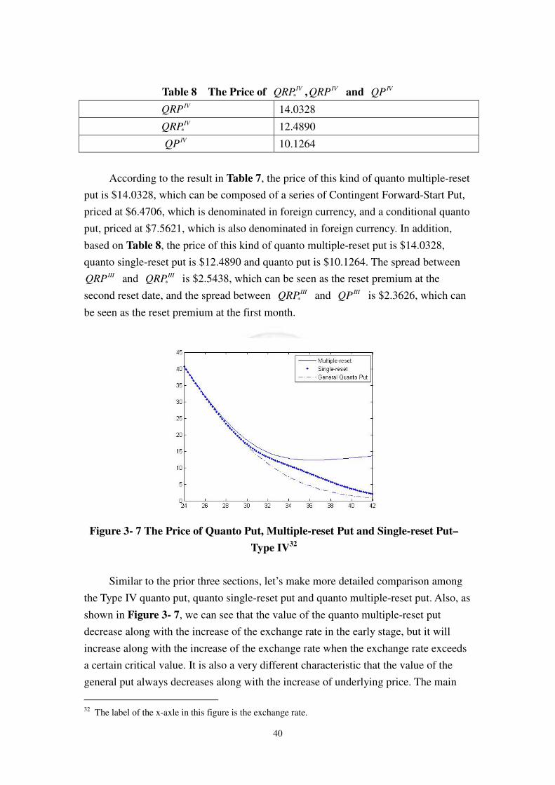
Figure 3- 7 The Price of Quanto Put, Multiple-reset Put and Single-reset Put–
Type IV32
Similar to the prior three sections, let’s make more detailed comparison among
the Type IV quanto put, quanto single-reset put and quanto multiple-reset put. Also, as
shown in Figure 3- 7, we can see that the value of the quanto multiple-reset put
decrease along with the increase of the exchange rate in the early stage, but it will
increase along with the increase of the exchange rate when the exchange rate exceeds
a certain critical value. It is also a very different characteristic that the value of the
general put always decreases along with the increase of underlying price. The main
32 The label of the x-axle in this figure is the exchange rate.
41
reason is the same as which we explain in the prior three sections, so we don’t
describe it again.
Now, we’ll go on to analyze the characteristic of the risk of the Type IV quanto
multiple-reset put.
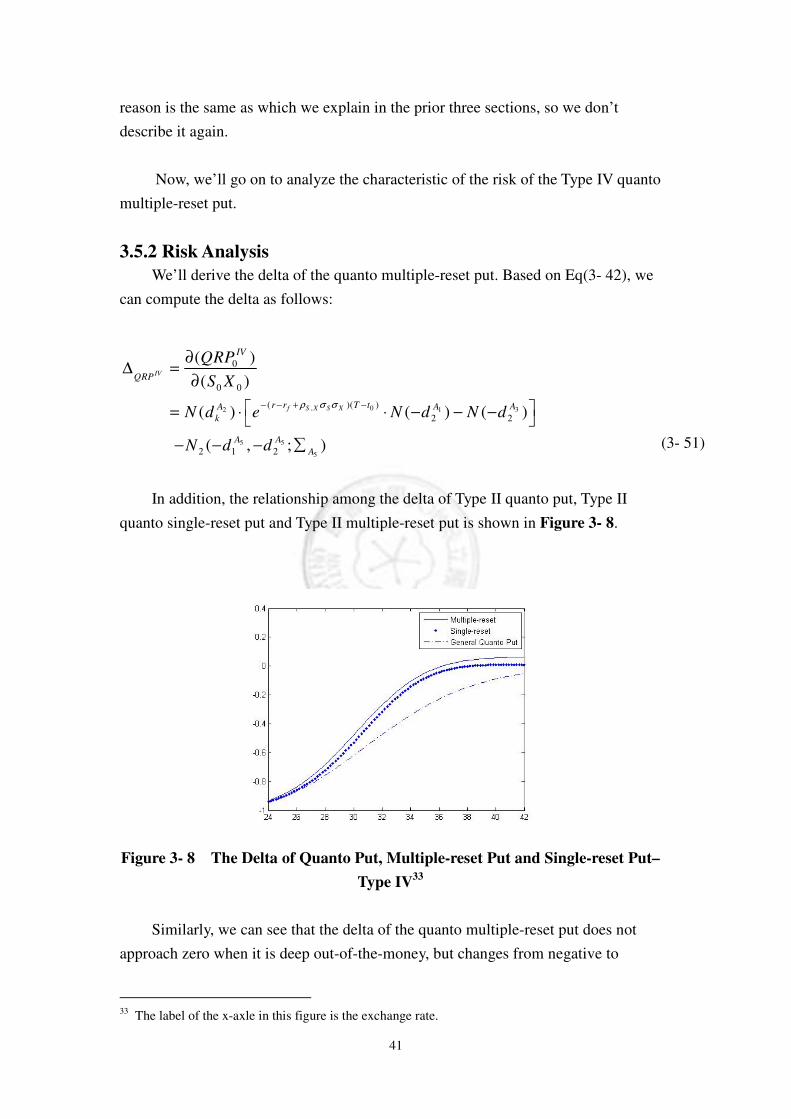
3.5.2 Risk Analysis
We’ll derive the delta of the quanto multiple-reset put. Based on Eq(3- 42), we
can compute the delta as follows:
In addition, the relationship among the delta of Type II quanto put, Type II
quanto single-reset put and Type II multiple-reset put is shown in Figure 3- 8.
Figure 3- 8 The Delta of Quanto Put, Multiple-reset Put and Single-reset Put–
Type IV33
Similarly, we can see that the delta of the quanto multiple-reset put does not
approach zero when it is deep out-of-the-money, but changes from negative to
33 The label of the x-axle in this figure is the exchange rate.
, 0 32 1
5 5
5
0
0 0
( )( )
2 2
2 1 2
( )
( )
( ) ( ) ( )
( , ; )
IV
f S X S X
IV
QRP
r r T t AA A
k
A A
A
QRP
S X
N d e N d N d
N d d
ρ σ σ− − + −
∂∆ =
∂
= ⋅ ⋅ − − −
− − − ∑
(3- 51)

42
positive. On the other hand, the delta of the quanto single-reset put is also positive
when it is deep out-of-the-money, but the magnitude of it is not as large as that of the
quanto multiple-reset put. The main reason is the same as which we explain in the
prior three sections, so we don’t describe it again.