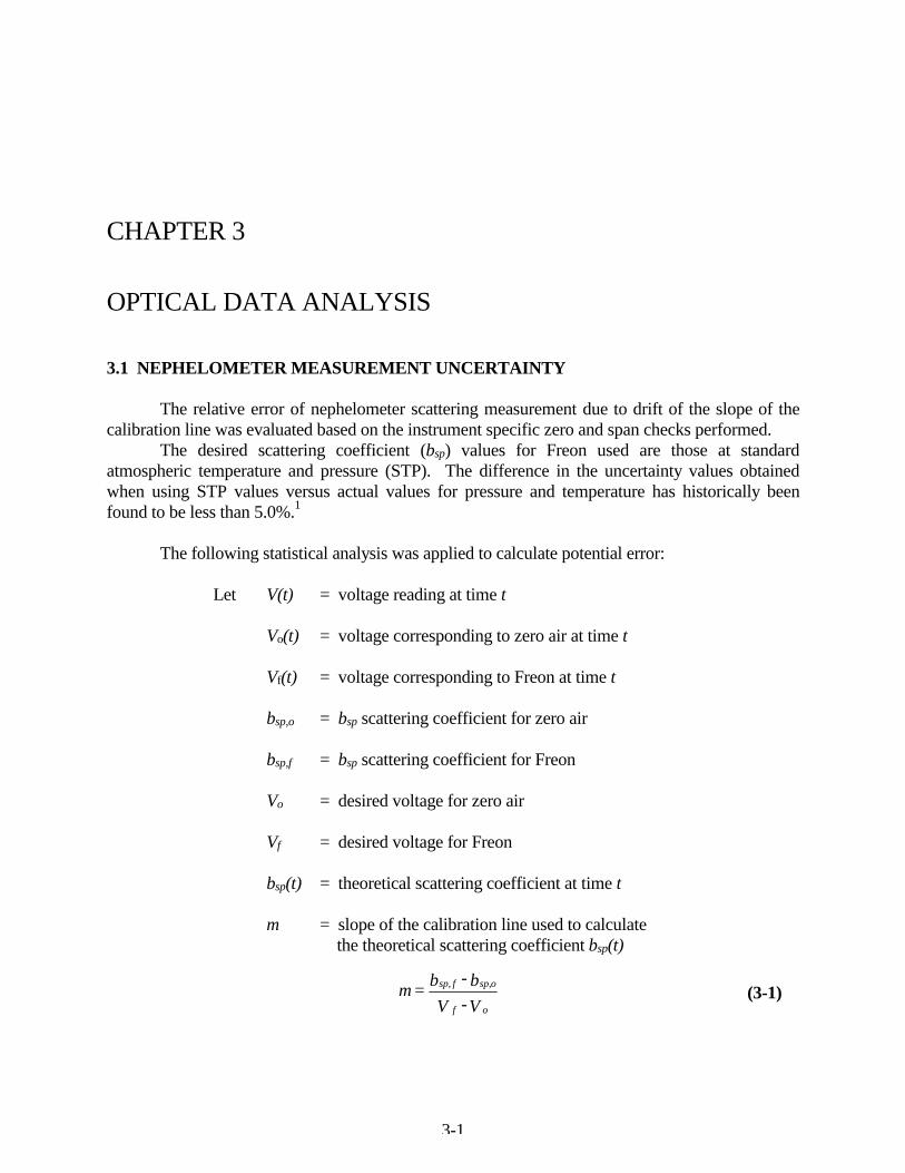
3-1

CHAPTER 3 OPTICAL DATA ANALYSIS 3.1 NEPHELOMETER MEASUREMENT UNCERTAINTY The relative error of nephelometer scattering measurement due to drift of the slope of the calibration line was evaluated based on the instrument specific zero and span checks performed. The desired scattering coefficient (bsp) values for Freon used are those at standard atmospheric temperature and pressure (STP). The difference in the uncertainty values obtained when using STP values versus actual values for pressure and temperature has historically been found to be less than 5.0%.1 The following statistical analysis was applied to calculate potential error: Let V(t) = voltage reading at time t Vo(t) = voltage corresponding to zero air at time t Vf(t) = voltage corresponding to Freon at time t bsp,o = bsp scattering coefficient for zero air bsp,f = bsp scattering coefficient for Freon Vo = desired voltage for zero air Vf = desired voltage for Freon bsp(t) = theoretical scattering coefficient at time t m = slope of the calibration line used to calculate the theoretical scattering coefficient bsp(t)

V - Vb - b = m

of

osp,fsp, (3-1)

3-2

Given a voltage reading V(t), the theoretical bsp at time t is:

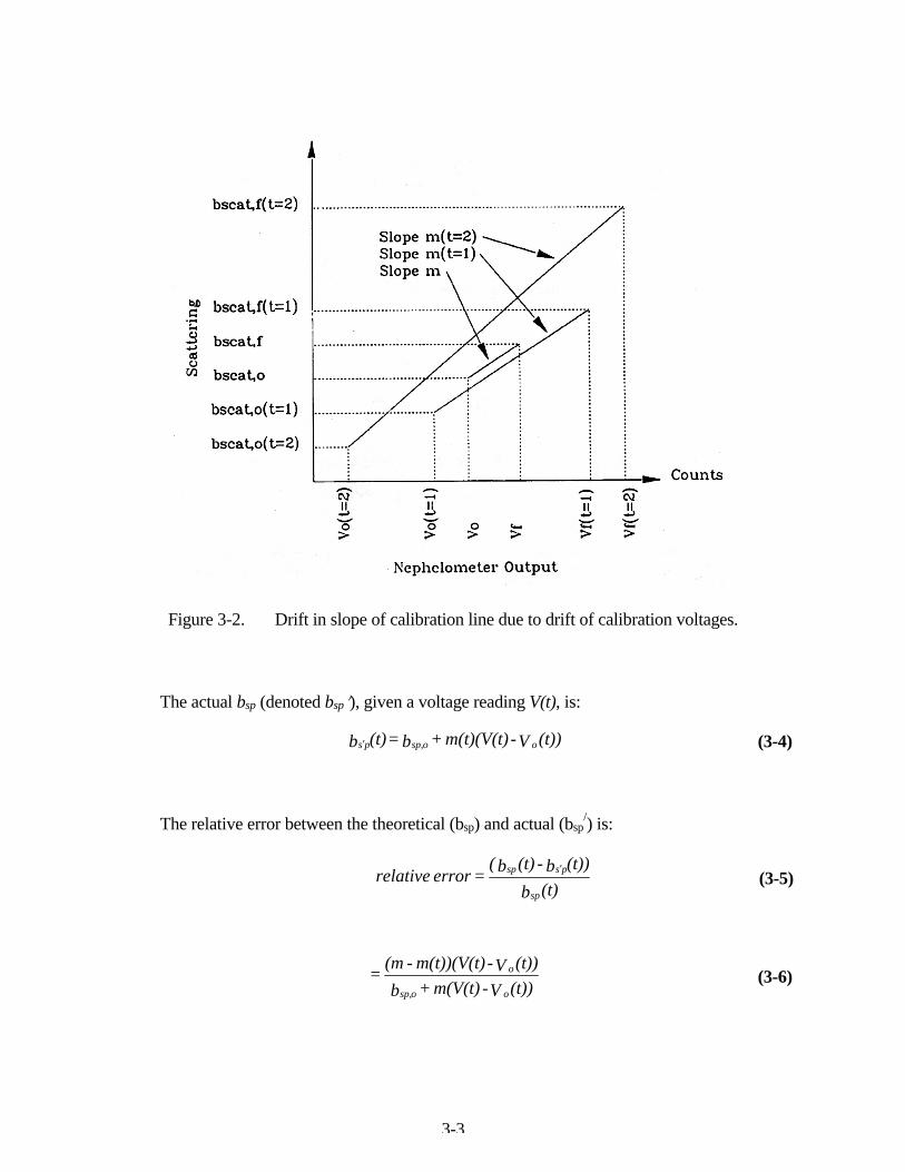
assuming that Vo(t) and V(t) are known without error. This is reasonable because these values are usually calculated by interpolating between automatic zero readings. The slope of the calibration line is not constant as is defined above but changes (drifts) with time. Figure 3-1 illustrates the drift in the zero air and span voltages with time. Figure 3-2 illustrates how these drifting voltages cause the slope of the calibration line to drift. The actual slope of the calibration line at time t is:

Figure 3-1. Drift in the zero air and Freon voltages with time.

(t))V - m(V(t) + b = (t)b oosp,sp (3-2)

(t)V - (t)V()b - b(

= m(t)of

osp,fsp, (3-3)

3-3

Figure 3-2. Drift in slope of calibration line due to drift of calibration voltages. The actual bsp (denoted bspN), given a voltage reading V(t), is:

The relative error between the theoretical (bsp) and actual (bsp

/) is:

(t)b(t))b - (t)b(

= error relativesp

pssp ′ (3-5)

(t))V - m(t)(V(t) + b = (t)b oosp,ps′ (3-4)

(t))V - m(V(t) + b(t))V - m(t))(V(t) - (m =

oosp,

o (3-6)

3-4

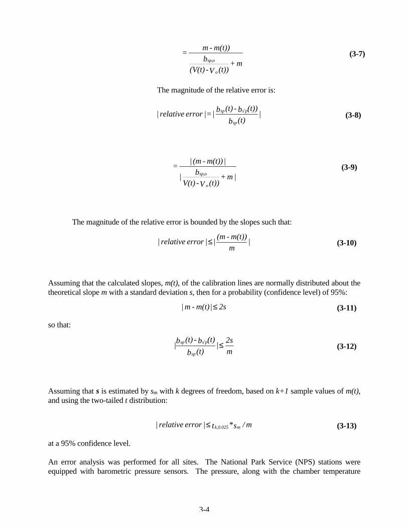
The magnitude of the relative error is:

The magnitude of the relative error is bounded by the slopes such that:

Assuming that the calculated slopes, m(t), of the calibration lines are normally distributed about the theoretical slope m with a standard deviation s, then for a probability (confidence level) of 95%:

so that:

Assuming that s is estimated by sm with k degrees of freedom, based on k+1 sample values of m(t), and using the two-tailed t distribution:

at a 95% confidence level. An error analysis was performed for all sites. The National Park Service (NPS) stations were equipped with barometric pressure sensors. The pressure, along with the chamber temperature

m +

(t))V - (V(t)b

m(t)) - m =

o

osp, (3-7)

|m +

(t))V - V(t)b|

|m(t)) - (m| =

o

osp, (3-9)

|(t)b

(t))b - (t)b| = |error relative|sp

pssp ′ (3-8)

|mm(t)) - (m| |error relative| ≤ (3-10)

2s |m(t) - m| ≤ (3-11)

m2s |

(t)b(t)b - (t)b|

sp

pssp ≤′ (3-12)

m/ s*t |error relative| mk,0.025≤ (3-13)

3-5

during Freon calibration, was used to calculate the expected Freon scattering value. For each NPS station, an error analysis was performed with Freon values obtained by both the altitude method and the pressure/temperature method. Results of the error analysis for each site are summarized in Table 3-1. Table 3-1. Summary of the error analysis for 1990 PREVENT study nephelometers.

Site Location Relative Error Percent (%)

Method

Dog Mountain 14.3 Altitude South Mountain 12.5 Altitude Tahoma Woods 9.0 Pressure/Temperature Tahoma Woods 9.0 Altitude Paradise 34.5 Altitude Carbon River 5.1 Pressure/Temperature Carbon River 6.9 Altitude Marblemount 32.0 Pressure/Temperature Marblemount 30.7 Altitude Newhalem 15.6 Altitude

3.1.1 Nephelometer Station Meteorological and Support Sensors Meteorological and support sensors (nephelometer inlet and chamber thermocouples) were checked for correct operation prior to installation and during the take-down. All sensors performed well. No periodic checks of sensor operation were made throughout the PREVENT study. 3.1.2 Nephelometer Operating Temperature Considerations The three NPS nephelometers (Tahoma, Carbon River, and Marblemount) operated with sample chamber temperatures that were kept as close as possible to the ambient temperature. This was accomplished by the following: C Inlet canes were kept short and were covered with reflective (silver) tape. C Nephelometers were housed in small (4'l x 4'w x 8'h) stand-alone shelters

equipped with a high air flow fan (1500 cfm). The fan circulated ambient air through the shelter, after first passing through a moisture trap and a dust filter. The inside of the shelter was maintained at temperatures very close to ambient.

C Nephelometers were equipped with medium size muffin fans (150 cfm)

3-6

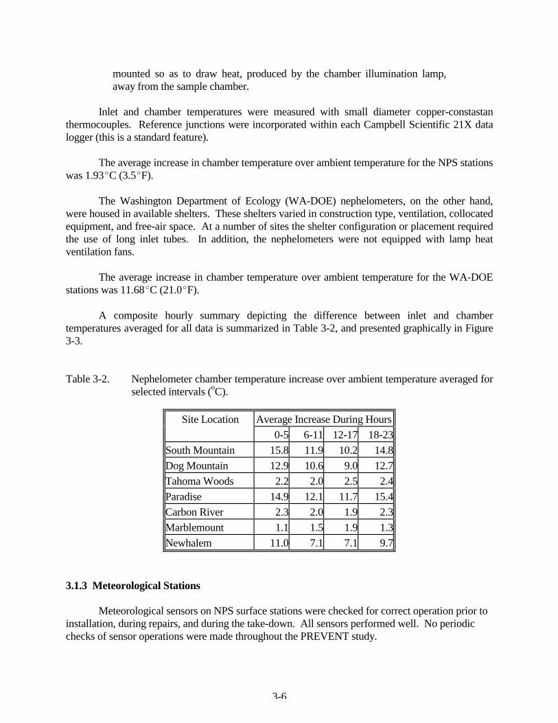
mounted so as to draw heat, produced by the chamber illumination lamp, away from the sample chamber.

Inlet and chamber temperatures were measured with small diameter copper-constastan thermocouples. Reference junctions were incorporated within each Campbell Scientific 21X data logger (this is a standard feature). The average increase in chamber temperature over ambient temperature for the NPS stations was 1.93EC (3.5EF). The Washington Department of Ecology (WA-DOE) nephelometers, on the other hand, were housed in available shelters. These shelters varied in construction type, ventilation, collocated equipment, and free-air space. At a number of sites the shelter configuration or placement required the use of long inlet tubes. In addition, the nephelometers were not equipped with lamp heat ventilation fans. The average increase in chamber temperature over ambient temperature for the WA-DOE stations was 11.68EC (21.0EF). A composite hourly summary depicting the difference between inlet and chamber temperatures averaged for all data is summarized in Table 3-2, and presented graphically in Figure 3-3. Table 3-2. Nephelometer chamber temperature increase over ambient temperature averaged for

selected intervals (oC).

Site Location Average Increase During Hours 0-5 6-11 12-17 18-23South Mountain 15.8 11.9 10.2 14.8Dog Mountain 12.9 10.6 9.0 12.7Tahoma Woods 2.2 2.0 2.5 2.4Paradise 14.9 12.1 11.7 15.4Carbon River 2.3 2.0 1.9 2.3Marblemount 1.1 1.5 1.9 1.3Newhalem 11.0 7.1 7.1 9.7

3.1.3 Meteorological Stations Meteorological sensors on NPS surface stations were checked for correct operation prior to installation, during repairs, and during the take-down. All sensors performed well. No periodic checks of sensor operations were made throughout the PREVENT study.

3-7

Figure 3-3. Composite hourly summary, (inlet-chamber) temperature.

3-8

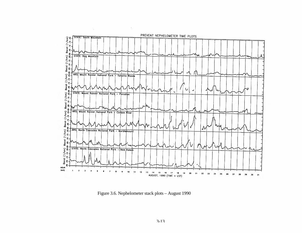
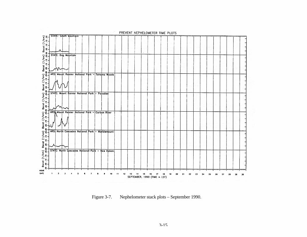
3.2 DESCRIPTIONS OF DATA PRESENTATIONS - NEPHELOMETER Hourly averaged nephelometer readings (bscat) are depicted by month for all monitoring stations in a plotting order which provides easy comparison between sites in similar regions. "Stack plots" for June, July, August and September are shown in Figures 3-4 through 3-7, respectively. Nephelometer data for the entire study period is summarized by site in seasonal summary plots (Figures 3-8 through 3-14). The plots and statistics are based on one-hour, averaged data. Data recovery statistics reported are for instrument operational periods, as opposed to the study period. Table 3-3 summarizes the standard visual range frequency of occurrence statistics which appear on the seasonal summary reports. Table 3-3. PREVENT study nephelometer data summary for the complete monitoring period.

Site Location

Frequency of Occurrence

10% 50% 90% bscat SVR bscat SVR bscat SVR

South Mountain .041 99 .026 160 .015 294 Dog Mountain .049 83 .030 139 .017 259 Tahoma Woods .084 48 .045 91 .021 210 Paradise .049 81 .027 149 .014 296 Carbon River .089 45 .049 83 .027 158 Marblemount .073 56 .040 105 .024 185 Newhalem .066 61 .034 123 .021 209

bscat units = (km-1), includes Rayleigh SVR = standard visual range (km) (2% contrast

3-9

Figure 3-4. Nephelometer stack plots – June 1990

3-11

Figure 3-5. Nephelometer stack plots – July 1990

3-13

Figure 3.6. Nephelometer stack plots – August 1990

3-15

Figure 3-7. Nephelometer stack plots – September 1990.

3-16

Figure 3-8. Nephelometer seasonal summary – Tahoma Woods.

Figure 3-9. Nephelometer seasonal summary – Dog Mountain.

Figure 3-10. Nephelometer seasonal summary – Tahoma Woods.

Figure 3-11. Nephelometer seasonal summary – Paradise.

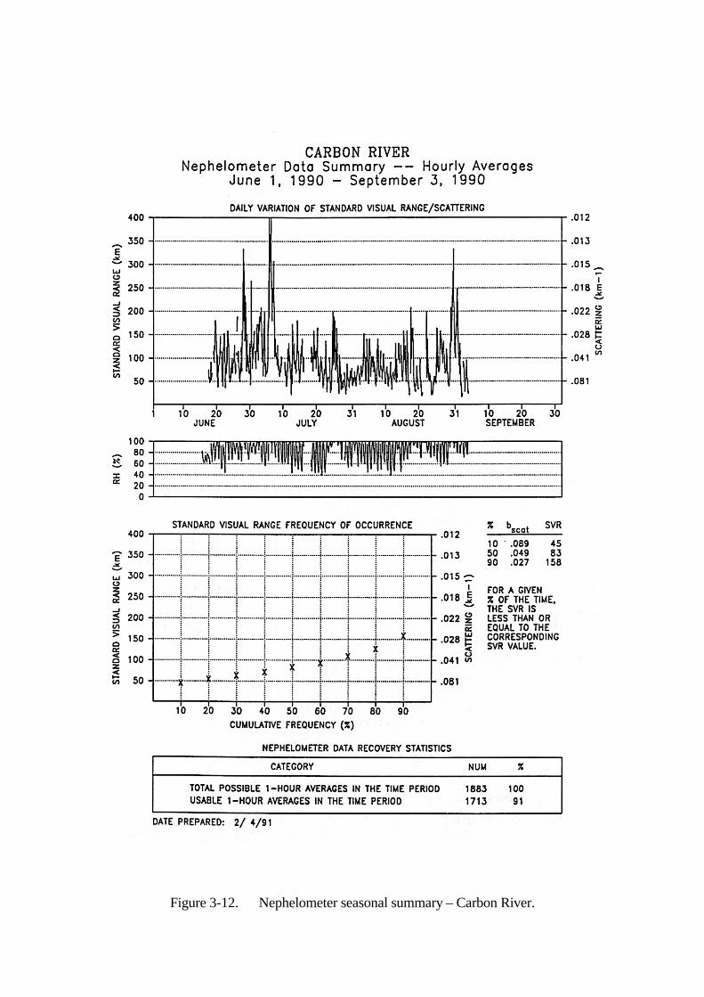
Figure 3-12. Nephelometer seasonal summary – Carbon River.

Figure 3-13. Nephelometer seasonal summary – Marblemount.

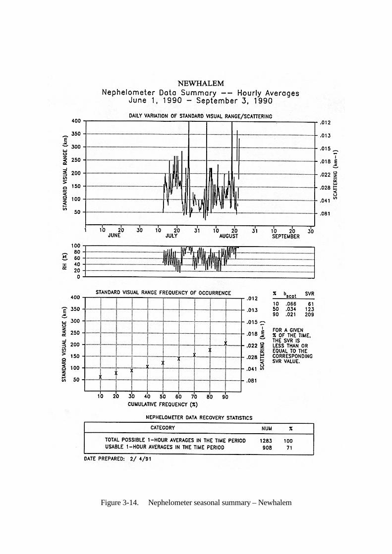
Figure 3-14. Nephelometer seasonal summary – Newhalem

REFERENCES 1. Molenar, J.V., D.S. Cismoski, and R.M. Tree, 1992. Intercomparison of ambient optical

monitoring techniques. Presented at the 85th Annual Meeting and Exhibition, Air and Waste Management. Kansas City, MO, Paper No. 92-60.09, June 21-26.