
CHAPTER 3: LARGE SAMPLE THEORY
118
CHAPTER 3: LARGE SAMPLE THEORY
Transcript of CHAPTER 3: LARGE SAMPLE THEORY

CHAPTER 3: LARGE SAMPLE THEORY

Introduction

•Why we need large sample theory For statistical inference, studying small or finite sample
property of statistics is usually difficult or tedious. A large sample (asymptotic) theory examines the limiting
behavior of a sequence of random variables, which usuallycan be well characterized by probability laws. Some well known results regarding sample mean:
Xn → µ,√
n(Xn − µ)→ N(0, σ2).
However, since Xn(ω) is a function on a probabilitymeasure space, it is important to be precise in terms ofwhat convergence mode.
In-class remark Non asymptotic results are also important, especially in high dimensional and machine learning
researches, but they are usually not exact.

Modes of Convergence

• Convergence almost surelyDefinition 3.1 Xn is said to converge almost surely to X, denotedby Xn →a.s. X, if there exists a set A ⊂ Ω such that P(Ac) = 0and for each ω ∈ A, Xn(ω)→ X(ω) in real space.
• Convergence in probabilityDefinition 3.2 Xn is said to converge in probability to X, denotedby Xn →p X, if for every ε > 0,
P(|Xn − X| > ε)→ 0.
• Convergence in moments/meansDefinition 3.3 Xn is said to converge in rth mean to X, denote byXn →r X, if
E[|Xn − X|r]→ 0 as n→∞ for functions Xn,X ∈ Lr(P),
where X ∈ Lr(P) means∫|X|rdP <∞.

• Equivalent condition for convergence almost surelySince
ω : Xn(ω)→ X(ω)c
= ∪ε>0 ∩n ω : supm≥n|Xm(ω)− X(ω)| > ε,
Xn →a.s. X if and only if
P(supm≥n|Xm − X| > ε)→ 0,
which is equivalent to
supm≥n|Xm − X| →p 0.

• Convergence in distributionDefinition 3.4 Xn is said to converge in distribution of X, denotedby Xn →d X or Fn →d F (or L(Xn)→ L(X) with L referring to the“law” or “distribution”), if the distribution functions Fn and Fof Xn and X satisfy
Fn(x)→ F(x) as n→∞ for each continuity point x of F.
In-class remark This convergence mode is unique to the sequence of random variables, and it plays the most
important role in statistical inference.

• Uniform integrabilityDefinition 3.5 A sequence of random variables Xn isuniformly integrable if
limλ→∞
lim supn→∞
E |Xn|I(|Xn| ≥ λ) = 0.
In-class remark This condition, although nothing to do with any specific convergence mode, is a useful condition toensure when studying the asymptotic limit of E[Xn], we only need to focus on the part where |Xn| < λ:Since
E[Xn] = E[XnI(|Xn| < λ)] + E[XnI(|Xn| ≥ λ)],
it holdslimλ→∞
lim supn|E[Xn]− E[XnI(|Xn| < λ)]| = 0.

• One sufficient condition to check the uniform integrability Liapunov condition: there exists a positive constant ε0 such
that lim supn E[|Xn|1+ε0 ] <∞. Usually, we choose ε0 = 0 so once the second moments of
Xn’s are uniformly bounded, Xn satisfies the uniformintegrability condition.
This is because
E[|Xn|I(|Xn| ≥ λ)] ≤ E[|Xn|1+ε0 |]λε0
.

• Remarks Convergence almost surely and convergence in probability
are the same as defined in measure theory. Two new definitions are ∗ convergence in rth mean and ∗
convergence in distribution. Mode, “convergence in distribution”, is very different from
the other modes since it only concerns the distribution ofXn, instead of the actual value/realization of Xn. Consider a sequence X,Y,X,Y,X,Y, .... where X and Y are
N(0, 1); the sequence converges in distribution to N(0, 1)but the other modes do not hold. “Convergence in distribution” is important for the
asymptotic statistical inference which mostly concernsabout the distribution behavior.

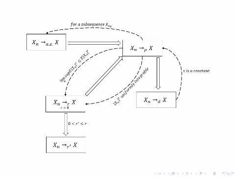
• Relationship among different modesTheorem 3.1A. If Xn →a.s. X, then Xn →p X.
B. If Xn →p X, then Xnk →a.s. X for some subsequence Xnk .
C. If Xn →r X, then Xn →p X.
D. If Xn →p X and |Xn|r is uniformly integrable, then Xn →r X.
E. If Xn →p X and lim supn E|Xn|r ≤ E|X|r, then Xn →r X.

F. If Xn →r X, then Xn →r′ X for any 0 < r′ ≤ r.
G. If Xn →p X, then Xn →d X.
H. Xn →p X if and only if for every subsequence Xnk thereexists a further subsequence Xnk,l such that Xnk,l →a.s. X.
I. If Xn →d c for a constant c, then Xn →p c.

Proof of Theorem 3.1
A and B follow from the results in the measure theory.
Prove C. It follows fromMarkov inequality: for any increasing function g(·) and random variable Y,
P(|Y| > ε) ≤ E[g(|Y|)g(ε)
].
Thus,
⇒P(|Xn − X| > ε) ≤ E[|Xn − X|r
εr]→ 0.
Prove D. It is sufficient to show that for any subsequence of Xn, there exists a further subsequence Xnk suchthat E[|Xnk − X|r]→ 0.
For any subsequence of Xn, from B, there exists a further subsequence Xnk such that Xnk →a.s. X. For any ε,there exists λ such that
lim supnk
E[|Xnk |rI(|Xnk |
r ≥ λ)] < ε.
We can further choose λ such that P(|X|r = λ) = 0 (why?). Thus
|Xnk |rI(|Xnk |
r ≥ λ)→a.s. |X|rI(|X|r ≥ λ).
By the Fatou’s Lemma, we conclude
E[|X|rI(|X|r ≥ λ)] ≤ lim supnk
E[|Xnk |rI(|Xnk |
r ≥ λ)] < ε.

Therefore,
E[|Xnk − X|r]
≤ E[|Xnk − X|rI(|Xnk |r< 2λ, |X|r < 2λ)]
+E[|Xnk − X|rI(|Xnk |r ≥ 2λ, or , |X|r ≥ 2λ)]
≤ E[|Xnk − X|rI(|Xnk |r< 2λ, |X|r < 2λ)]
+2rE[(|Xnk |r+ |X|r)I(|Xnk |
r ≥ 2λ, or , |X|r ≥ 2λ)],
where the last inequality follows from the inequality (x + y)r ≤ 2r(max(x, y))r ≤ 2r(xr + yr), x ≥ 0, y ≥ 0.
When nk is large, the second term is bounded by
2r
E[|Xnk |rI(|Xnk |
r ≥ λ)] + E[|X|rI(|X|r ≥ λ)]≤ 2r+1
ε.
Therefore, lim supn E[|Xnk − X|r] ≤ 2r+1ε since the first term vanishes by DCT. We have proved D.

Prove E. It is sufficient to show that for any subsequence of Xn, there exists a further subsequence Xnk suchthat E[|Xnk − X|r]→ 0.
For any subsequence of Xn, there exists a further subsequence Xnk such that Xnk →a.s. X. Define
Ynk = 2r(|Xnk |
r+ |X|r)− |Xnk − X|r ≥ 0.
By the Fatou’s Lemma, ∫lim inf
nkYnk dP ≤ lim inf
nk
∫Ynk dP.
It is equivalent to
2r+1E[|X|r] ≤ lim infnk
2rE[|Xnk |
r] + 2rE[|X|r]− E[|Xnk − X|r]
.

Prove F. We will use the Holder inequality:
∫|f(x)g(x)|dµ ≤
∫|f(x)|pdµ(x)
1/p ∫|g(x)|pdµ(x)
1/q,
p, q > 0,1
p+
1
q= 1.
Choose µ = P, f = |Xn − X|r′, g ≡ 1 and p = r/r′, q = r/(r− r′) in the Holder inequality to obtain
E[|Xn − X|r′] ≤ E[|Xn − X|r]r′/r → 0.

Prove G. Xn →p X. If P(X = x) = 0, then for any ε > 0,
P(|I(Xn ≤ x)− I(X ≤ x)| > ε)
= P(|I(Xn ≤ x)− I(X ≤ x)| > ε, |X − x| > δ)
+P(|I(Xn ≤ x)− I(X ≤ x)| > ε, |X − x| ≤ δ)≤ P(Xn ≤ x,X > x + δ) + P(Xn > x,X < x− δ)
+P(|X − x| ≤ δ)≤ P(|Xn − X| > δ) + P(|X − x| ≤ δ).
The first term converges to zero since Xn →p X. The second term can be arbitrarily small if δ is small, since
limδ→0
P(|X − x| ≤ δ) = P(X = x) = 0.
Thus, we obtain I(Xn ≤ x)→p I(X ≤ x) so Fn(x) = E[I(Xn ≤ x)]→ E[I(X ≤ x)] = F(x) by DCT.

Prove H. One direction follows from B.
We use the contradiction to prove the other direction. Suppose there exists ε > 0 such that P(|Xn − X| > ε) doesnot converge to zero. Thus, we can find a subsequence Xn′ such hat P(|Xn′ − X| > ε) > δ for some δ > 0.However, by the condition, there exists a further subsequence Xn′′ in Xn′ such that Xn′′ →a.s. X thenXn′′ →p X from A. Then P(|Xn′′ − X| > ε)→ 0, leading to a contradiction.
Prove I. Let X ≡ c. ThenP(|Xn − c| > ε) ≤ 1− Fn(c + ε) + Fn(c− ε)
Note that the RHS converges to1− FX(c + ε) + F(c− ε) = 0.

• Counter-examples
(Example 1) X1,X2, ... are i.i.d with standard normaldistribution. Then Xn →d X1 but Xn does not converge inprobability to X1.
(Example 2) Let Z be a random variable with a uniformdistribution in [0, 1]. Let Xn = I(m2−k ≤ Z < (m + 1)2−k) whenn = 2k + m where 0 ≤ m < 2k. Then it is shown that Xnconverges in probability to zero but not almost surely. Thisexample was also given in the second chapter.
(Example 3) Let Z be Uniform(0, 1) and letXn = 2nI(0 ≤ Z < 1/n). Then E[|Xn|r]]→∞ but Xn converges tozero almost surely.

•More results for convergence in rth meanTheorem 3.2 (Vitali’s theorem) Suppose that Xn ∈ Lr(P), i.e.,‖Xn‖r <∞, where 0 < r <∞ and Xn →p X. Then the followingare equivalent:
A. |Xn|r are uniformly integrable.
B. Xn →r X.
C. E[|Xn|r]→ E[|X|r].In-class remark The proof uses similar techniques in the proof of Theorem 3.1.

Integral inequalities

• Young’s inequality Let p, q > 0 and 1/p + 1/q = 1 (p and q arecalled conjugate numbers). Then for any a, b,
|ab| ≤ |a|p
p+|b|q
q, a, b > 0,
where the equality holds if and only if |a|p = |b|q.
Proof of Young’s inequality Since log x is concave,
log(1p|a|p +
1q|b|q) ≥ 1
plog |a|p +
1q
log |b|.
The equality holds iff |a|p = |b|q.In-class remark There is a geometric interpretation of the inequality by plotting the curve y = xp−1 in the square
[0, |a|]× [0, |b|].

• Holder inequality∫|f (x)g(x)|dµ(x) ≤
∫|f (x)|pdµ(x)
1p∫|g(x)|qdµ(x)
1q
.
Proof of Holder inequality In the Young’s inequality, leta = f (x)/
∫|f (x)|pdµ(x)
1/p b = g(x)/∫|g(x)|qdµ(x)
1/q, andthen integrate both sides of the inequality.
When µ = P, f = X(ω) and g = 1, µs−tr µr−s
t ≥ µr−ts where
µr = E[|X|r] and r ≥ s ≥ t ≥ 0. When p = q = 2, we obtain Cauchy-Schwartz inequality:∫
|f (x)g(x)|dµ(x) ≤∫
f (x)2dµ(x)
12∫
g(x)2dµ(x)
12
.

•Minkowski’s inequality r > 1,
‖X + Y‖r ≤ ‖X‖r + ‖Y‖r.
Proof of Minkowski’s inequality It follows from the Holderinequality that
E[|X + Y|r] ≤ E[(|X|+ |Y|)|X + Y|r−1]
≤ E[|X|r]1/rE[|X + Y|r]1−1/r + E[|Y|r]1/rE[|X + Y|r]1−1/r.
This implies that ‖ · ‖r forms a norm in the linear spaceX : ‖X‖r <∞. Such a normed space is denoted as Lr(P).

•Markov’s inequality For any ε > 0,
P(|X| ≥ ε) ≤ E[g(|X|)]g(ε)
,
where g ≥ 0 is a increasing function in [0,∞).Proof of Markov’s inequality It follows from
P(|X| ≥ ε) ≤ P(g(|X|) ≥ g(ε))
= E[I(g(|X|) ≥ g(ε))]
≤ E[g(|X|)g(ε)
].
When g(x) = x2 and X replaced by X − E[X], we obtainChebyshev’s inequality:
P(|X − E[X]| ≥ ε) ≤ Var(X)
ε2 .
It is the simplest result among the so-called concentrationinequalities (probability concentrated around its mean)and this holds for any distributions.

• Asymptotic limit of sample mean statistic Y1,Y2, ... are i.i.d with mean µ and variance σ2. Let
Xn = Yn. By the Chebyshev’s inequality,
P(|Xn − µ| > ε) ≤ Var(Xn)
ε2 =σ2
nε2 → 0.
As a result,Xn →p µ.
From the Liapunov condition with r = 1 and ε0 = 1,|Xn − µ| satisfies the uniform integrability condition. Thenfrom the Vitali’s theorem, we obtain
E[|Xn − µ|]→ 0.
In other words, the sample mean converges to the truemean in the first moment.

Convergence in Distribution

“Convergence in distribution is the most important mode ofconvergence for statistical inference.”
Recall Xn →d X if Fn(x)→ F(x) for x ∈ C(F), where C(F) is theset of all continuity points of F. Sometimes, we write C(X) forC(F).

Equivalent definitionsTheorem 3.3 (Portmanteau Theorem) The following conditionsare equivalent.
(a). Xn converges in distribution to X.
(b). For any bounded continuous function g(·),
E[g(Xn)]→ E[g(X)].
(c). For any open set G in R, lim infn P(Xn ∈ G) ≥ P(X ∈ G).
(d). For any closed set F in R, lim supn P(Xn ∈ F) ≤ P(X ∈ F).
(e). For any Borel set O in R with P(X ∈ ∂O) = 0 where ∂O isthe boundary of O, P(Xn ∈ O)→ P(X ∈ O).

Proof of Theorem 3.3
(a)⇒(b). Without loss of generality, assume |g(x)| ≤ 1. We choose [−M,M] such that P(|X| = M) = 0.
Since g is continuous in [−M,M], g is uniformly continuous in [−M,M].
We partition [−M,M] into finite intervals I1 ∪ ... ∪ Im such that within each interval Ik ,maxIk
g(x)− minIkg(x) ≤ ε and X has no mass at all the endpoints of Ik (why?).
Therefore, if choose any point xk ∈ Ik, k = 1, ...,m,
|E[g(Xn)]− E[g(X)]|≤ E[|g(Xn)|I(|Xn| > M)] + E[|g(X)|I(|X| > M)]
+|E[g(Xn)I(|Xn| ≤ M)]−m∑
k=1
g(xk)P(Xn ∈ Ik)|
+|m∑
k=1
g(xk)P(Xn ∈ Ik)−m∑
k=1
g(xk)P(X ∈ Ik)|
+|E[g(X)I(|X| ≤ M)]−m∑
k=1
g(xk)P(X ∈ Ik)|
≤ P(|Xn| > M) + P(|X| > M)
+2ε +m∑
k=1
|P(Xn ∈ Ik)− P(X ∈ Ik)|.
We obtain lim supn |E[g(Xn)]− E[g(X)]| ≤ 2P(|X| > M) + 2ε. Let M→∞ and ε→ 0 to complete the proof.

(b)⇒(c). For any open set G, define
g(x) = 1−ε
ε + d(x,Gc),
where d(x,Gc) is the minimal distance between x and Gc , i.e., infy∈Gc |x− y|.
For any y ∈ Gc ,d(x1,Gc
)− |x2 − y| ≤ |x1 − y| − |x2 − y| ≤ |x1 − x2|,
so d(x1,Gc)− d(x2,Gc) ≤ |x1 − x2|. Therefore,
|g(x1)− g(x2)| ≤ ε−1|d(x1,Gc)− d(x2,Gc
)| ≤ ε−1|x1 − x2|.
Thus, g(x) is continuous and bounded, so (b) implies
E[g(Xn)]→ E[g(X)].
Note 0 ≤ g(x) ≤ IG(x) solim inf
nP(Xn ∈ G) ≥ lim inf
nE[g(Xn)]→ E[g(X)].
Finally, let ε→ 0 then E[g(X)] converges to E[I(X ∈ G)] = P(X ∈ G).
(c)⇒(d). This is clear by considering G = Fc in (c). In fact, (c) and (d) are equivalent.

(c)&(d)⇒(e). For any O with P(X ∈ ∂O) = 0,
lim supn
P(Xn ∈ O) ≤ lim supn
P(Xn ∈ O) ≤ P(X ∈ O) = P(X ∈ O),
andlim inf
nP(Xn ∈ O) ≥ lim inf
nP(Xn ∈ Oo
) ≥ P(X ∈ Oo) = P(X ∈ O).
(e)⇒(a). Choose O = (−∞, x] with P(X ∈ ∂O) = P(X = x) = 0. Then (a) follows from the result in (e).

• Counter examples Let g(x) = x, a continuous but unbounded function. Let Xn
be a random variable taking value n with probability 1/nand value 0 with probability (1− 1/n). Then Xn →d 0.However, E[g(Xn)] = 1 does not converge to 0.
The continuity at boundary in (e) is also necessary: let Xnbe degenerate at 1/n and consider O = x : x > 0. ThenP(Xn ∈ O) = 1 but Xn →d 0.

Weak Convergence and Characteristic Function

Theorem 3.4 (Continuity Theorem) Let φn and φ denote thecharacteristic functions of Xn and X respectively. Then Xn →d Xis equivalent to φn(t)→ φ(t) for each t.
Proof of Theorem 3.4To prove⇒ direction, from (b) in Theorem 3.1, we have
φn(t) = E[eitXn ]→ E[eitX] = φ(t).
The proof of⇐ direction uses the Helly selection and result that Xn is asymptotically tight. We skip the proof.

• One simple exampleAssume X1, ...,Xn ∼ Bernoulli(p). Then
φXn(t) = E[eit(X1+...+Xn)/n] = (1 = p + peit/n)n
= (1− p + p + itp/n + o(1/n))n → eitp.
Note the limit is the c.f. of X = p. Thus, Xn →d p so Xnconverges in probability to p.

• Generalization to multivariate random vectors
Xn →d X if and only if E[expit′Xn]→ E[expit′X], wheret is any k-dimensional constant. Equivalently, t′Xn →d t′X for any t. Hence, to study the weak convergence of random vectors,
it is sufficient to study the weak convergence ofone-dimensional (any) linear combination of the randomvectors. This is the well-known Cramer-Wold’s device:
Theorem 3.5 (The Cramer-Wold device) Random vectorXn in Rk satisfy Xn →d X if and only t′Xn →d t′X in R for allt ∈ Rk.

Properties of Weak Convergence

Theorem 3.6 (Continuous mapping theorem) SupposeXn →a.s. X, or Xn →p X, or Xn →d X. Then for any continuousfunction g(·), g(Xn) converges to g(X) almost surely, or inprobability, or in distribution.

Proof of Theorem 3.6
Clearly, if Xn →a.s. X, then Xn(ω)→ X(ω) for ω ∈ A for some set A with P(A) = 1. Since g is continuous,g(Xn(ω))→ g(X(ω)) for ω ∈ A. That is, g(Xn)→a.s g(X).
If Xn →p X, then for any subsequence, there exists a further subsequence Xnk →a.s. X. Thus, g(Xnk )→a.s. g(X).Hence, g(Xn)→p g(X) according to (H) in Theorem 3.1.
To prove that g(Xn)→d g(X) when Xn →d X, we directly verify (b) in the Portmanteau Theorem.

• One remarkTheorem 3.6 concludes that g(Xn)→d g(X) if Xn →d X and g iscontinuous. In fact, this result still holds if P(X ∈ C(g)) = 1where C(g) contains all the continuity points of g. That is, if it isimpossible for X to take values at g’s discontinuity points, thecontinuous mapping theorem holds.

Theorem 3.7 (Slutsky theorem) Suppose Xn →d X, Yn →p yand Zn →p z for some constant y and z. ThenZnXn + Yn →d zX + y.
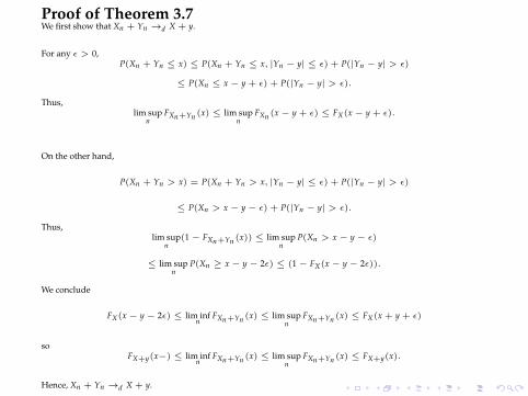
Proof of Theorem 3.7We first show that Xn + Yn →d X + y.
For any ε > 0,P(Xn + Yn ≤ x) ≤ P(Xn + Yn ≤ x, |Yn − y| ≤ ε) + P(|Yn − y| > ε)
≤ P(Xn ≤ x− y + ε) + P(|Yn − y| > ε).
Thus,lim sup
nFXn+Yn (x) ≤ lim sup
nFXn (x− y + ε) ≤ FX(x− y + ε).
On the other hand,
P(Xn + Yn > x) = P(Xn + Yn > x, |Yn − y| ≤ ε) + P(|Yn − y| > ε)
≤ P(Xn > x− y− ε) + P(|Yn − y| > ε).
Thus,lim sup
n(1− FXn+Yn (x)) ≤ lim sup
nP(Xn > x− y− ε)
≤ lim supn
P(Xn ≥ x− y− 2ε) ≤ (1− FX(x− y− 2ε)).
We conclude
FX(x− y− 2ε) ≤ lim infn
FXn+Yn (x) ≤ lim supn
FXn+Yn (x) ≤ FX(x + y + ε)
soFX+y(x−) ≤ lim inf
nFXn+Yn (x) ≤ lim sup
nFXn+Yn (x) ≤ FX+y(x).
Hence, Xn + Yn →d X + y.

To complete the proof, we note
P(|(Zn − z)Xn| > ε) ≤ P(|Zn − z| > ε2) + P(|Zn − z| ≤ ε2
, |Xn| >1
ε).
As a result,lim sup
nP(|(Zn − z)Xn| > ε) ≤ lim sup
nP(|Zn − z| > ε
2)
+ lim supn
P(|Xn| ≥1
2ε) ≤ P(|X| ≥
1
2ε).
This implies (Zn − z)Xn →p 0.
Clearly, zXn →d zX soZnXn = (Zn − z)Xn + zXn →d zX
from the proof in the first half. Using the first half’s proof again, we obtain
ZnXn + Yn →d zX + y.

• Alternative Proof
First, show (Xn, Yn)→d (X, y).
|φ(Xn,Yn)(t1, t2)− φ(X,y)(t1, t2)| = |E[eit1Xn eit2Yn ]− E[eit1Xeit2y]|
≤ |E[eit1Xn (eit2Yn − eit2y)]| + |eit2y||E[eit1Xn ]− E[eit1X
]|
≤ E[|eit2Yn − eit2y|] + |E[eit1Xn ]− E[eit1X]| → 0.
Similarly, (Zn,Xn)→d (z,X). Since g(z, x) = zx is continuous,
ZnXn →d zX.
Since (ZnXn, Yn)→d (zX, y) and g(x, y) = x + y is continuous,
ZnXn + Yn →d zX + y.

• Examples
Suppose Xn →d N(0, 1). Then by continuous mappingtheorem, X2
n →d χ21.
The condition Yn →p y, where y is a constant, is necessary.For example, let Xn = X ∼ N(0, 1) then Xn →d −X. LetYn = X so Yn →p X. However Xn + Yn = 2X does notconverge in distribution to −X + X = 0.

Let X1,X2, ... be a random sample from a normaldistribution with mean µ and variance σ2 > 0,
√n(Xn − µ)→d N(0, σ2),
s2n =
1n− 1
n∑i=1
(Xi − Xn)2 →a.s σ2.
Thus, √n(Xn − µ)
sn→d
1σ
N(0, σ2) ∼= N(0, 1).
In other words, in a large sample, tn−1 can beapproximated by a standard normal distribution.

Representation of Weak Convergence

Theorem 3.8 (Skorohod’s Representation Theorem) Let Xnand X be random variables in a probability space (Ω,A,P) andXn →d X. Then there exists another probability space (Ω, A, P)and a sequence of random variables Xn and X defined on thisspace such that Xn and Xn have the same distributions, X and Xhave the same distributions, and moreover, Xn →a.s. X.

• The proof relies on quantile function
F−1(p) = infx : F(x) ≥ p.
Proposition 3.1
(a) F−1 is left-continuous.
(b) If X has continuous distribution function F, then
F(X) ∼ Uniform(0, 1).
(c) Let ξ ∼ Uniform(0, 1) and let X = F−1(ξ). Then for all x,X ≤ x = ξ ≤ F(x). Thus, X has distribution function F.

Proof of Proposition 3.1
(a) Clearly, F−1 is nondecreasing. Suppose pn increases to p then F−1(pn) increases to some y ≤ F−1(p). ThenF(y) ≥ pn so F(y) ≥ p. We have F−1(p) ≤ y so y = F−1(p).
(b) Note that X ≤ x ⊂ F(X) ≤ F(x). It gives
F(x) ≤ P(F(X) ≤ F(x)).
On the other hand,F(X) ≤ F(x)− ε ⊂ X ≤ x
givesP(F(X) ≤ F(x)− ε) ≤ F(x).
Thus, P(F(X) ≤ F(x)−) ≤ F(x). Since X is continuous, we conclude P(F(X) ≤ F(x)) = F(x).
(c) This follows fromP(X ≤ x) = P(F−1
(ξ) ≤ x) = P(ξ ≤ F(x)) = F(x).

Proof of Theorem 3.8
Let (Ω, A, P) be ([0, 1],B ∩ [0, 1], λ). Define Xn = F−1n (ξ), X = F−1(ξ), where ξ ∼ Uniform(0, 1). Xn has a
distribution Fn which is the same as Xn .
For any t ∈ (0, 1) such that there is at most one value x such that F(x) = t (it is easy to see this if t is the continuouspoint of F−1), for any z < x, F(z) < t so when n is large, Fn(z) < t and F−1
n (t) ≥ z. We thus havelim infn F−1
n (t) ≥ z so lim infn F−1n (t) ≥ x = F−1(t).
From F(x + ε) > t, Fn(x + ε) > t so F−1n (t) ≤ x + ε. Thus, lim supn F−1
n (t) ≤ x + ε and lim supn F−1n (t) ≤ x.
This implies that F−1n (t)→ F−1(t) for almost every t ∈ (0, 1). Thus, Xn →a.s. X.

• Usefulness of representation theorem
For example, if Xn →d X and one wishes to show somefunction of Xn, denote by g(Xn), converges in distributionto g(X), we can use the following “detour” steps:
find a representation, Xn and X, which shares the samedistribution with Xn and X respectively. Furthermore, Xnconverges to X almost surely; establish the desired result for Xn and X. In this case,
g(Xn)→d g(X); since the distributions of g(Xn) and g(X) are identical to
g(Xn) and g(X) respectively, g(Xn)→d g(X) holds.

• Diagram of the proof using resprentation
↓ Xn →d X ? ⇒ ? g(Xn) →d g(X) ↑↓ ⇑ ↑↓ g(Xn) →d g(X) ↑↓ ⇑ ↑↓ Xn →a.s. X ⇒ g(Xn) →a.s. g(X) ↑→ → → → → → →

Summation of Independent Random Variables

• Some preliminary lemmasProposition 3.2 (Borel-Cantelli Lemma) For any events An,
∞∑i=1
P(An) <∞
implies P(An, i.o.) = P(An occurs infinitely often) = 0; orequivalently, P(∩∞n=1 ∪m≥n Am) = 0.Proof of Propositon 3.2
P(An, i.o) ≤ P(∪m≥nAm) ≤∑m≥n
P(Am)→ 0, as n→∞.

• One important result of the first Borel-cantelli lemmaIf for a sequence of random variables, Zn, and for any ε > 0,∑
n P(|Zn| > ε) <∞, then |Zn| > ε only occurs finite times.Hence,
Zn →a.s. 0.

Proposition 3.3 (Second Borel-Cantelli Lemma) For asequence of independent events A1,A2, ...,
∑∞n=1 P(An) =∞
implies P(An, i.o.) = 1.Proof of Proposition 3.3 Consider the complement of An, i.o.
P(∪∞n=1 ∩m≥n Acm) = lim
nP(∩m≥nAc
m) = limn
∏m≥n
(1− P(Am))
≤ lim supn
exp−∑m≥n
P(Am) = 0.

• Equivalence lemmaProposition 3.4 Assume that X1, ...,Xn are i.i.d with finitemean. Define Yn = XnI(|Xn| ≤ n). Then
∞∑n=1
P(Xn 6= Yn) <∞.

Proof of Proposition 3.4 Since E[|X1|] <∞,
∞∑n=1
P(|X| ≥ n) =
∞∑n=1
nP(n ≤ |X| < (n + 1)) ≤∞∑
n=1
E[|X|] <∞.
From the Borel-Cantelli Lemma, P(Xn 6= Yn, i.o) = 0.
For almost every ω ∈ Ω, when n is large enough,
Xn(ω) = Yn(ω).
That is, the asymptotic behavior of Xn is the same as the oneof Yn.

Weak Law of Large Number

Theorem 3.9 (Weak Law of Large Number, WLLN) IfX,X1, ...,Xn are i.i.d with mean µ (so E[|X|] <∞ and µ = E[X]),then Xn →p µ.
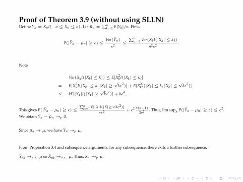
Proof of Theorem 3.9 (without using SLLN)Define Yn = XnI(−n ≤ Xn ≤ n). Let µn =
∑nk=1 E[Yk]/n. First,
P(|Yn − µn| ≥ ε) ≤Var(Yn)
ε2≤∑n
k=1 Var(XkI(|Xk| ≤ k))
n2ε2.
Note
Var(XkI(|Xk| ≤ k)) ≤ E[X2k I(|Xk| ≤ k)]
= E[X2k I(|Xk| ≤ k, |Xk| ≥
√kε2
)] + E[X2k I(|Xk| ≤ k, |Xk| ≤
√kε2
)]
≤ kE[|Xk|I(|Xk| ≥√
kε2)] + kε4
,
This gives P(|Yn − µn| ≥ ε) ≤∑n
k=1 E[|X|I(|X|≥√
kε2)]
nε2 + ε2 n(n+1)2n2 . Thus, lim supn P(|Yn − µn| ≥ ε) ≤ ε2 .
We obtain Yn − µn →p 0.
Since µn → µ, we have Yn →p µ.
From Proposition 3.4 and subsequence arguments, for any subsequence, there exits a further subsequence,
Ynk →a.s. µ so Xnk →a.s. µ. Thus, Xn →p µ.

Strong Law of Large Number

Theorem 3.10 (Strong Law of Large Number, SLLN) IfX1, ...,Xn are i.i.d with mean µ then Xn →a.s. µ.

Proof of Theorem 3.10
Without loss of generality, we assume Xn ≥ 0 since if this is true, the result also holds for any Xn byXn = X+
n − X−n .
By equivalence lemma, it is sufficient to show Yn →a.s. µ, where Yn = XnI(Xn ≤ n). NoteE[Yn] = E[X1I(X1 ≤ n)]→ µ so
n∑k=1
E[Yk]/n→ µ.
Therefore, if we denote Sn =∑n
k=1(Yk − E[Yk]), then it suffices to show Sn/n→a.s. 0.
Note
Var(Sn) =n∑
k=1
Var(Yk) ≤n∑
k=1
E[Y2k ] ≤ nE[X2
1I(X1 ≤ n)].
By the Chebyshev’s inequality,
P(|Sn
n| > ε) ≤
1
n2ε2Var(Sn) ≤
E[X21I(X1 ≤ n)]
nε2.
For any α > 1, let un = [αn].
∞∑n=1
P(|Sun
un| > ε) ≤
∞∑n=1
1
unε2E[X2
1I(X1 ≤ un)]
≤1
ε2E[X2
1
∑un≥X1
1
un].

Since for any x > 0,∑
un≥xµn−1 < 2∑
n≥log x/ logα α−n ≤ Kx−1 for some constant K,
∞∑n=1
P(|Sun
un| > ε) ≤
K
ε2E[X1] <∞,
we conclude Sun/un →a.s. 0.For any k, we can find un < k ≤ un+1 . Thus, since X1,X2, ... ≥ 0,
Sun
un
un
un+1≤
Sk
k≤
Sun+1
un+1
un+1
un.
It gives
µ/α ≤ lim infk
Sk
k≤ lim sup
k
Sk
k≤ µα.
Since α is arbitrary number larger than 1, let α→ 1 and we obtain limk Sk/k = µ.

Central Limit Theorems

• Preliminary result of c.f.Proposition 3.5 Suppose E[|X|m] <∞ for some integer m ≥ 0.Then
|φX(t)−m∑
k=0
(it)k
k!E[Xk]|/|t|m → 0, as t→ 0.
Proof of Proposition 3.5Note
eitx=
m∑k=1
(itx)k
k!+
(itx)m
m![eitθx − 1],
where θ ∈ [0, 1]. We have
|φX(t)−m∑
k=0
(it)k
k!E[Xk
]|/|t|m ≤ E[|X|m|eitθX − 1|]/m!→ 0,
as t→ 0.

• Classical CLTTheorem 3.11 (Central Limit Theorem) If X1, ...,Xn are i.i.dwith mean µ and variance σ2 then
√n(Xn − µ)→d N(0, σ2).
Proof of Theorem 3.11 Denote Yn =√
n(Xn − µ).
φYn (t) =φX1−µ(t/
√n)n.
Note φX1−µ(t/√
n) = 1− σ2t2/2n + o(1/n) so
φYn (t)→ exp−σ2t2
2.

Theorem 3.12 (Multivariate Central Limit Theorem) IfX1, ...,Xn are i.i.d random vectors in Rk with mean µ andcovariance Σ = E[(X−µ)(X−µ)′], then
√n(Xn−µ)→d N(0,Σ).
Proof of Theorem 3.12 It is directly from applying the Cramer-Wold’s device.

• Liaponov CLTTheorem 3.13 (Liapunov Central Limit Theorem) LetXn1, ...,Xnn be independent random variables with µni = E[Xni]and σ2
ni = Var(Xni). Let µn =∑n
i=1 µni, σ2n =
∑ni=1 σ
2ni. If
n∑i=1
E[|Xni − µni|3]
σ3n
→ 0,
then∑n
i=1(Xni − µni)/σn →d N(0, 1).

• Lindeberg-Feller CLTTheorem 3.14 (Lindeberg-Fell Central Limit Theorem) LetXn1, ...,Xnn be independent random variables with µni = E[Xni]and σ2
ni = Var(Xni). Let σ2n =
∑ni=1 σ
2ni. Then both
n∑i=1
(Xni − µni)/σn →d N(0, 1)
andmax
σ2
ni/σ2n : 1 ≤ i ≤ n
→ 0
if and only if the Lindeberg condition
1σ2
n
n∑i=1
E[|Xni − µni|2I(|Xni − µni| ≥ εσn)]→ 0 for all ε > 0
holds.
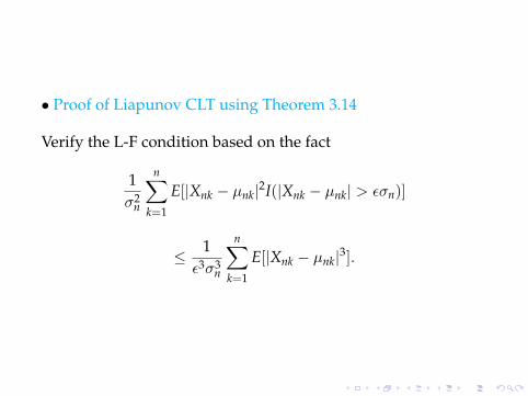
• Proof of Liapunov CLT using Theorem 3.14
Verify the L-F condition based on the fact
1σ2
n
n∑k=1
E[|Xnk − µnk|2I(|Xnk − µnk| > εσn)]
≤ 1ε3σ3
n
n∑k=1
E[|Xnk − µnk|3].

•Weighted CLTTheorem 3.14.2 (Weighted Central Limit Theorem) LetX1, ...,Xn be i.i.d with mean µ and variance σ2. For anysequence of weights wn1, ...,wnn satisfying
maxi|wni|√∑ni=1 w2
ni
→ 0,
it holds ∑ni=1 wni(Xi − µ)
σ√∑n
i=1 w2ni
→d N(0, 1).

• Proof of Theorem 3.14.2 by verifying the L-F condition:
Let σ2n = σ2 ∑n
i=1 w2ni .
1
σ2n
n∑k=1
E[|wnk(Xk − µ)|2I(|wnk(Xk − µ)| > εσn)]
≤1
σ2n
n∑k=1
w2nkE[|(Xk − µ)|2I(|Xk − µ| >
εσn
maxk |wnk|)]
=1
σ2E[|(X1 − µ)|2I(|X1 − µ| >
εσn
maxk |wnk|)]
→ 0.

• Examples
This is one example from a simple linear regressionXj = α+ βzj + εj for j = 1, 2, ... where zj are knownnumbers not all equal and the εj are i.i.d with mean zeroand variance σ2.
βn =
n∑j=1
Xj(zj − zn)/
n∑j=1
(zj − zn)2
= β +
n∑j=1
εj(zj − zn)/
n∑j=1
(zj − zn)2.
Assume
maxj≤n
(zj − zn)2/
n∑j=1
(zj − zn)2 → 0.
⇒√
n√∑n
j=1(zj−zn)2
n (βn − β)→d N(0, σ2) by weighted CLT.

The example is taken from the randomization test forpaired comparison. Let (Xj,Yj) denote the values of jthpairs with Xj being the result of the treatment andZj = Xj − Yj. Conditional on |Zj| = zj, Zj = |Zj|sgn(Zj) isindependent taking values ±|Zj|with probability 1/2,when treatment and control have no difference. Conditional on z1, z2, ... (zj can be very different among
pairs), the randomization t-test is the t-statistic√n− 1Zn/sz where s2
z is 1/n∑n
j=1(Zj − Zn)2. Note (Rj = sgn(Zj))
Zn = n−1n∑
j=1
zjRj, s2z = n−1
n∑j=1
z2j − (n−1
n∑j=1
zjRj)2.
When
maxj≤n
z2j /
n∑j=1
z2j → 0,
this statistic has an asymptotic normal distribution N(0, 1)(by weighted CLT).

Delta Method
Theorem 3.15 (Delta method) For random vector X and Xn inRk , if there exists two constant an and µ such thatan(Xn − µ)→d X and an →∞, then for any function g : Rk 7→ Rl
such that g has a derivative at µ, denoted by∇g(µ)
an(g(Xn)− g(µ))→d ∇g(µ)X.

Proof of Theorem 3.15
By the Skorohod representation, we can construct Xn and X such that Xn ∼d Xn and X ∼d X (∼d means the samedistribution) and an(Xn − µ)→a.s. X.Since g is differentiable at µ,
an(g(Xn)− g(µ))→a.s. ∇g(µ)X.
Thus,an(g(Xn)− g(µ))→d ∇g(µ)X.
Since an(g(Xn)− g(µ)) has the same distribution as an(g(Xn)− g(µ)), we conclude
an(g(Xn)− g(µ))→d ∇g(µ)X.

• Examples
Let X1,X2, ... be i.i.d with fourth moment ands2
n = (1/n)∑n
i=1(Xi − Xn)2. Denote mk as the kth moment ofX1 for k ≤ 4. Note that s2
n = (1/n)∑n
i=1 X2i − (
∑ni=1 Xi/n)2
and√
n[(
Xn(1/n)
∑ni=1 X2
i
)−(
m1m2
)]→d N
(0,(
m2 −m1 m3 −m1m2m3 −m1m2 m4 −m2
2
)),
the Delta method with g(x, y) = y− x2 gives theasymptotic distribution for
√n(s2
n − Var(X1)).

Let (X1,Y1), (X2,Y2), ... be i.i.d bivariate samples withfinite fourth moment. One estimate of the correlationamong X and Y is
ρn =sxy√s2
xs2y
,
where sxy = (1/n)∑n
i=1(Xi − Xn)(Yi − Yn),s2
x = (1/n)∑n
i=1(Xi − Xn)2 and s2y = (1/n)
∑ni=1(Yi − Yn)2.
To derive the large sample distribution of ρn, first obtainthe large sample distribution of (sxy, s2
x, s2y) using the Delta
method then further apply the Delta method withg(x, y, z) = x/√yz.

The example is taken from the Pearson’s Chi-squarestatistic. Suppose that one subject falls into K categorieswith probabilities p1, ..., pK, where p1 + ...+ pK = 1. ThePearson’s statistic is defined as
χ2 = nK∑
k=1
(nk
n− pk)
2/pk,
which can be treated as∑(observed count− expected count)2/expected count.
Note√
n(n1/n− p1, ...,nK/n− pK) has an asymptoticmultivariate normal distribution. Then we can apply thecontinuous mapping theorem, instead of the Deltamethod, to g(x1, ..., xK) =
∑Ki=1 x2
k .

U-statistics

• DefinitionDefinition 3.6 A U-statistics associated with h(x1, ..., xr) isdefined as
Un =1
r!(n
r
)∑β
h(Xβ1 , ...,Xβr),
where the sum is taken over the set of all unordered subsets βof r different integers chosen from 1, ...,n.

• Examples
One simple example is h(x, y) = xy. ThenUn = (n(n− 1))−1∑
i 6=j XiXj.
Un = E[h(X1, ...,Xr)|X(1), ...,X(n)].
Un is the summation of non-independent randomvariables. If define h(x1, ..., xr) as (r!)−1∑
(x1,...,xr)h(x1, ..., xr), then
h(x1, ..., xr) is permutation-symmetric
Un =1(nr
) ∑β1<...<βr
h(β1, ..., βr).
h is called the kernel of the U-statistic Un.

• CLT for U-statisticsTheorem 3.16 Let µ = E[h(X1, ...,Xr)]. If E[h(X1, ...,Xr)
2] <∞,then
√n(Un − µ)−
√n
n∑i=1
E[Un − µ|Xi]→p 0.
Consequently,√
n(Un − µ) is asymptotically normal with meanzero and variance r2σ2, where, with X1, ...,Xr, X1, ..., Xr i.i.dvariables,
σ2 = Cov(h(X1,X2, ...,Xr), h(X1, X2, ..., Xr)).

• Some preparation Linear space of r.v.:let S be a linear space of random
variables with finite second moments that contain theconstants; i.e., 1 ∈ S and for any X,Y ∈ S, aX + bY ∈ Snwhere a and b are constants. Projection: for random variable T, a random variable S is
called the projection of T on S if E[(T − S)2] minimizesE[(T − S)2], S ∈ S.

Proposition 3.7 Let S be a linear space of random variableswith finite second moments. Then S is the projection of T on Sif and only if S ∈ S and for any S ∈ S, E[(T − S)S] = 0. Everytwo projections of T onto S are almost surely equal. If the linearspace S contains the constant variable, then E[T] = E[S] andCov(T − S, S) = 0 for every S ∈ S.

Proof of Proposition 3.7
For any S and S in S,E[(T − S)
2] = E[(T − S)
2] + 2E[(T − S)S] + E[(S− S)
2].
If S satisfies that E[(T − S)S] = 0, then E[(T − S)2] ≥ E[(T − S)2]. That is, S is the projection of T on S.
If S is the projection, for any constant α, E[(T − S− αS)2] is minimized at α = 0. Calculate the derivative atα = 0 to obtain E[(T − S)S] = 0.
If T has two projections S1 and S2 , then E[(S1 − S2)2] = 0. Thus, S1 = S2, a.s. If the linear space S contains the
constant variable, choose S = 1 gives 0 = E[(T − S)S] = E[T]− E[S]. Clearly,
Cov(T − S, S) = E[(T − S)S] = 0.

• Equivalence with projectionProposition 3.8 Let Sn be linear space of random variables withfinite second moments that contain the constants. Let Tn berandom variables with projections Sn on to Sn. IfVar(Tn)/Var(Sn)→ 1 then
Zn ≡Tn − E[Tn]√
Var(Tn)− Sn − E[Sn]√
Var(Sn)→p 0.

Proof of Proposition 3.8
Clearly, E[Zn] = 0. Note that
Var(Zn) = 2− 2Cov(Tn, Sn)√
Var(Tn)Var(Sn).
Since Sn is the projection of Tn , Cov(Tn, Sn) = Cov(Tn − Sn, Sn) + Var(Sn) = Var(Sn). We have
Var(Zn) = 2(1−
√Var(Sn)
Var(Tn))→ 0.
By the Markov’s inequality, we conclude that Zn →p 0.

• Conclusion
if Sn is the summation of i.i.d random variables such that
(Sn − E[Sn])/√
Var(Sn)→d N(0, σ2),
so is(Tn − E[Tn])/
√Var(Tn).
The limit distribution of U-statistics is derived using thislemma.

• Proof of Theorem 3.16
Let X1, ..., Xr be random variables with the same distribution as X1 and they are independent of X1, ...,Xn .Denote Un by
∑ni=1 E[U − µ|Xi].
We show that Un is the projection of Un on the linear space
Sn =
g1(X1) + ... + gn(Xn) : E[gk(Xk)2] <∞, k = 1, ..., n
, which contains the constant variables. Clearly,
Un ∈ Sn . For any gk(Xk) ∈ Sn ,
E[(Un − Un)gk(Xk)] = E[E[Un − Un|Xk]gk(Xk)] = 0.
From
Un =r
n
n∑i=1
E[h(X1, ..., Xr−1,Xi)− µ|Xi],
we calculate
Var(Un) =r2
nCov(E[h(X1, ..., Xr−1,X1)|X1], E[h(X1, ..., Xr−1,X1)|X1]) =
r2σ2
n.

Furthermore,
Var(Un)
=
(n
r
)−2 ∑β
∑β′
Cov(h(Xβ1, ...,Xβr ), h(Xβ′1
, ...,Xβ′r))
=
(n
r
)−2 r∑k=1
∑β and β′ share k components
Cov(h(X1,X2, ..,Xk,Xk+1, ...,Xr), h(X1,X2, ...,Xk, Xk+1, ..., Xr)).
Thus,
Var(Un) =r∑
k=1
r!
k!(r− k)!
(n− r)(n− r + 1) · · · (n− 2r + k + 1)
n(n− 1) · · · (n− r + 1)ck.
That is, Var(Un) = r2n Cov(h(X1,X2, ...,Xr), h(X1, X2, ..., Xr)) + O( 1
n2 ).
Thus,Var(Un)/Var(Un)→ 1
soUn − µ√Var(Un)
−Un√
Var(Un)
→p 0.
We obtain the result.

• Example
In a bivariate i.i.d sample (X1,Y1), (X2,Y2), ..., one statisticof measuring the agreement is called Kendall’s τ -statistic
τ =4
n(n− 1)
∑∑i<j
I
(Yj − Yi)(Xj − Xi) > 0− 1.
⇒ τ + 1 is a U-statistic of order 2 with the kernel
2I (y2 − y1)(x2 − x1) > 0 .
⇒√
n(τn + 1− 2P((Y2 − Y1)(X2 − X1) > 0)) has anasymptotic normal distribution with mean zero.

Rank Statistics

• Some definitions X(1) ≤ X(2) ≤ ... ≤ X(n) is called order statistics The rank statistics, denoted by R1, ...,Rn are the ranks of Xi
among X1, ...,Xn. Thus, if all the X’s are different,Xi = X(Ri). When there are ties, Ri is defined as the average of all
indices such that Xi = X(j) (sometimes called midrank). Only consider the case that X’s have continuous densities.

•More definitions
a rank statistic is any function of the ranks a linear rank statistic is a rank statistic of the special form∑n
i=1 a(i,Ri) for a given matrix (a(i, j))n×n. if a(i, j) = ciaj, then such statistic with form
∑ni=1 ciaRi is
called simple linear rank statistic: c and a’s are called thecoefficients and scores.

• Examples In two independent sample X1, ...,Xn and Y1, ...,Ym, a
Wilcoxon statistic is defined as the summation of all theranks of the second sample in the pooled data X1, ...,Xn,Y1, ...,Ym, i.e.,
Wn =
n+m∑i=n+1
Ri.
Other choices for rank statistics: for instance, the van derWaerden statistic
∑n+mi=n+1 Φ−1(Ri).

• Properties of rank statisticsProposition 3.9 Let X1, ...,Xn be a random sample fromcontinuous distribution function F with density f . Then
1. the vectors (X(1), ...,X(n)) and (R1, ...,Rn) are independent;2. the vector (X(1), ...,X(n)) has density n!
∏ni=1 f (xi) on the set
x1 < ... < xn;3. the variable X(i) has density
(n−1i−1
)F(x)i−1(1− F(x))n−if (x);
for F the uniform distribution on [0, 1], it has meani/(n + 1) and variance i(n− i + 1)/[(n + 1)2(n + 2)];
4. the vector (R1, ...,Rn) is uniformly distributed on the set ofall n! permutations of 1, 2, ...,n;
5. for any statistic T and permutation r = (r1, ..., rn) of1, 2, ...,n,
E[T(X1, ...,Xn)|(R1, ..,Rn) = r] = E[T(X(r1), ..,X(rn))];
6. for any simple linear rank statistic T =∑n
i=1 ciaRi ,
E[T] = ncnan, Var(T) =1
n− 1
n∑i=1
(ci − cn)2n∑
i=1
(ai − an)2.

• CLT of rank statisticsTheorem 3.17 Let Tn =
∑ni=1 ciaRi such that
maxi≤n|ai−an|/
√√√√ n∑i=1
(ai − an)2 → 0, maxi≤n|ci−cn|/
√√√√ n∑i=1
(ci − cn)2 → 0.
Then (Tn − E[Tn])/√
Var(Tn)→d N(0, 1) if and only if for everyε > 0,
∑(i,j)
I
√n|ai − an||ci − cn|√∑n
i=1(ai − an)2∑n
i=1(ci − cn)2> ε
× |ai − an|2|ci − cn|2∑n
i=1(ai − an)2∑n
i=1(ci − cn)2 → 0.

•More on rank statistics a simple linear signed rank statistic
n∑i=1
aR+i
sign(Xi),
where R+1 , ...,R
+n , absolute rank, are the ranks of |X1|, ..., |Xn|.
In a bivariate sample (X1,Y1), ..., (Xn,Yn),∑n
i=1 aRibSi
where (R1, ...,Rn) and (S1, ...,Sn) are respective ranks of(X1, ...,Xn) and (Y1, ...,Yn).

Martingale

Definition 3.7 Let Yn be a sequence of random variables andFn be sequence of σ-fields such that F1 ⊂ F2 ⊂ .... SupposeE[|Yn|] <∞. Then the pairs (Yn,Fn) is called a martingale if
E[Yn|Fn−1] = Yn−1, a.s.
(Yn,Fn) is a submartingale if
E[Yn|Fn−1] ≥ Yn−1, a.s.
(Yn,Fn) is a supmartingale if
E[Yn|Fn−1] ≤ Yn−1, a.s.

• Some notes on definition Y1, ...,Yn are measurable in Fn. Sometimes, we say Yn is
adapted to Fn. One simple example: Yn = X1 + ...+ Xn, where X1,X2, ...
are i.i.d with mean zero, and Fn is the σ-filed generated byX1, ...,Xn.

• Convex function of martingalesProposition 3.9 Let (Yn,Fn) be a martingale. For anymeasurable and convex function φ, (φ(Yn),Fn) is asubmartingale.
Proof of Proposition 3.9
Clearly, φ(Yn) is adapted toFn . It is sufficient to show
E[φ(Yn)|Fn−1] ≥ φ(Yn−1).
This follows from the well-known Jensen’s inequality: for any convex function φ,
E[φ(Yn)|Fn−1] ≥ φ(E[Yn|Fn−1]) = φ(Yn−1).

• Jensen’s inequalityProposition 3.10 For any random variable X and any convexmeasurable function φ,
E[φ(X)] ≥ φ(E[X]).

Proof of Proposition 3.10
Claim that for any x0 , there exists a constant k0 such that for any x, φ(x) ≥ φ(x0) + k0(x− x0) (called supportinghyperplane).
By the convexity, for any x′ < y′ < x0 < y < x,
φ(x0)− φ(x′)
x0 − x′≤φ(y)− φ(x0)
y− x0≤φ(x)− φ(x0)
x− x0.
Thus,φ(x)−φ(x0)
x−x0is bounded and decreasing as x decreases to x0 . Let the limit be k+0 then we have
φ(x)−φ(x0)x−x0
≥ k+0 . That is,
φ(x) ≥ k+0 (x− x0) + φ(x0).
Similarly,φ(x′)− φ(x0)
x′ − x0≤φ(y′)− φ(x0)
y′ − x0≤φ(x)− φ(x0)
x− x0.
Thenφ(x′)−φ(x0)
x′−x0is increasing and bounded as x′ increases to x0 . Let the limit be k−0 to obtain
φ(x′) ≥ k−0 (x′ − x0) + φ(x0).
Clearly, k+0 ≥ k−0 . Combining those two inequalities,
φ(x) ≥ φ(x0) + k0(x− x0)
for k0 = (k+0 + k−0 )/2.
Finally, we choose x0 = E[X] then φ(X) ≥ φ(E[X]) + k0(X − E[X]).

• Decomposition of submartingale Yn = (Yn − E[Yn|Fn−1]) + E[Yn|Fn−1]
any submartingale can be written as the summation of amartingale and a random variable predictable in Fn−1.

• Convergence of martingalesTheorem 3.18 (Martingale Convergence Theorem) Let(Xn,Fn) be submartingale. If K = supn E[|Xn|] <∞, thenXn →a.s. X where X is a random variable satisfying E[|X|] ≤ K.
Corollary 3.1 If Fn is increasing σ-field and denote F∞ as theσ-field generated by ∪∞n=1Fn, then for any random variable Zwith E[|Z|] <∞, it holds
E[Z|Fn]→a.s. E[Z|F∞].

• CLT for martingaleTheorem 3.19 (Martingale Central Limit Theorem) Let(Yn1,Fn1), (Yn2,Fn2), ... be a martingale. DefineXnk = Ynk − Yn,k−1 with Yn0 = 0 thus Ynk = Xn1 + ...+ Xnk.Suppose that ∑
k
E[X2nk|Fn,k−1]→p σ
2
where σ is a positive constant and that∑k
E[X2nkI(|Xnk| ≥ ε)|Fn,k−1]→p 0
for each ε > 0. Then ∑k
Xnk →d N(0, σ2).

Notations in Asymptotic Arguments

• op(1) and Op(1)
Xn = op(1) denotes that Xn converges in probability to zero, Xn = Op(1) denotes that Xn is bounded in probability; i.e.,
limM→∞
lim supn
P(|Xn| ≥M) = 0.
for a sequence of random variable rn, Xn = op(rn) meansthat |Xn|/rn →p 0 and Xn = Op(rn) means that |Xn|/rn isbounded in probability.

• Algebra in op(1) and Op(1)
op(1) + op(1) = op(1) Op(1) + Op(1) = Op(1),
Op(1)op(1) = op(1) (1 + op(1))−1 = 1 + op(1)
op(Rn) = Rnop(1) Op(Rn) = RnOp(1)
op(Op(1)) = op(1).
If a real function R(·) satisfies that R(h) = o(|h|p) as h→ 0, then
R(Xn) = op(|Xn|p).
If R(h) = O(|h|p) as h→ 0, then R(Xn) = Op(|Xn|p).

READING MATERIALS: Lehmann and Casella, Section 1.8,Ferguson, Part 1, Part 2, Part 3 12-15


![[--------------------- ---------------------] Chapter 8 Interval Estimation n Interval Estimation of a Population Mean: Large-Sample Case Large-Sample.](https://static.fdocuments.in/doc/165x107/56649e895503460f94b8e9b8/-chapter-8-interval-estimation.jpg)


