Chapter 3 HIGHER ORDER SLIDING MODES

Chapter 3

HIGHER ORDER SLIDING

MODES

L. FRIDMAN� and A. LEVANT�� Chihuahua Institute of Technology, Chihuahua, Mexico.�� Institute for Industrial Mathematics, Beer-Sheva, Israel.

3.1 Introduction

One of the most important control problems is control under heavy un-certainty conditions. While there are a number of sophisticated methodslike adaptation based on identi�cation and observation, or absolute stabilitymethods, the most obvious way to withstand the uncertainty is to keep someconstraints by "brutal force". Indeed any strictly kept equality removes one"uncertainty dimension". The most simple way to keep a constraint is toreact immediately to any deviation of the system stirring it back to the con-straint by a su�ciently energetic e�ort. Implemented directly, the approachleads to so-called sliding modes, which became main operation modes in thevariable structure systems (VSS) [55]. Having proved their high accuracy androbustness with respect to various internal and external disturbances, theyalso reveal their main drawback: the so-called chattering e�ect, i.e. danger-ous high-frequency vibrations of the controlled system. Such an e�ect wasconsidered as an obvious intrinsic feature of the very idea of immediate pow-erful reaction to a minutest deviation from the chosen constraint. Anotherimportant feature is proportionality of the maximal deviation from the con-

1

2 CHAPTER 3. HIGHER ORDER SLIDING MODES

straint to the time interval between the measurements (or to the switchingdelay).

To avoid chattering some approaches were proposed [15, 51]. The mainidea was to change the dynamics in a small vicinity of the discontinuitysurface in order to avoid real discontinuity and at the same time to preservethe main properties of the whole system. However, the ultimate accuracyand robustness of the sliding mode were partially lost. Recently inventedhigher order sliding modes (HOSM) generalize the basic sliding mode ideaacting on the higher order time derivatives of the system deviation from theconstraint instead of in uencing the �rst deviation derivative like it happensin standard sliding modes. Keeping the main advantages of the originalapproach, at the same time they totally remove the chattering e�ect andprovide for even higher accuracy in realization. A number of such controllerswere described in the literature [16, 34, 35, 38, 3, 5].

HOSM is actually a movement on a discontinuity set of a dynamic sys-tem understood in Filippov's sense [22]. The sliding order characterizes thedynamics smoothness degree in the vicinity of the mode. If the task is toprovide for keeping a constraint given by equality of a smooth function sto zero, the sliding order is a number of continuous total derivatives of s(including the zero one) in the vicinity of the sliding mode. Hence, the rthorder sliding mode is determined by the equalities

s = _s = �s = ::: = s(r�1) = 0: (3.1)

forming an r-dimensional condition on the state of the dynamic system. Thewords "rth order sliding" are often abridged to "r-sliding".

The standard sliding mode on which most variable structure systems(VSS) are based is of the �rst order ( _s is discontinuous). While the standardmodes feature �nite time convergence, convergence to HOSM may be asymp-totic as well. r-sliding mode realization can provide for up to the rth orderof sliding precision with respect to the measurement interval [35, 38, 41]. Inthat sense r-sliding modes play the same role in sliding mode control theoryas Runge - Kutta methods in numerical integration. Note that such utmostaccuracy is observed only for HOSM with �nite-time convergence.

Trivial cases of asymptotically stable HOSM are easily found in manyclassic VSSs. For example there is an asymptotically stable 2-sliding modewith respect to the constraint x = 0 at the origin x = _x = 0 (at the one pointonly) of a 2-dimensional VSS keeping the constraint x+ _x = 0 in a standard

3.1. INTRODUCTION 3

1-sliding mode. Asymptotically stable or unstable HOSMs inevitably appearin VSSs with fast actuators [23, 25, 26, 27, 30]. Stable HOSM reveals itselfin that case by spontaneous disappearance of the chattering e�ect. Thus,examples of asymptotically stable or unstable sliding modes of any order arewell known [16, 14, 50, 35, 30]. On the contrary, examples of r-sliding modesattracting in �nite time are known for r = 1 (which is trivial), for r = 2[34, 16, 17, 35, 4, 5] and for r = 3 [30]. Arbitrary order sliding controllerswith �nite-time convergence were only recently presented [38, 41]. Any newtype of higher-order sliding controller with �nite-time convergence is uniqueand requires thorough investigation.

The main problem in implementation of HOSMs is increasing informationdemand. Generally speaking, any r-sliding controller keeping s = 0 needss; _s; :::; s(r�1) to be available. The only known exclusion is a so-called "super-twisting" 2-sliding controller [35, 37], which needs only measurements of s.First di�erences of s(r�2) having been used, measurements of s; _s; :::; s(r�2)

turned out to be su�cient, which solves the problem only partially. A re-cently published robust exact di�erentiator with �nite-time convergence [37]allows that problem to be solved in the theoretical way. In practice, however,the di�erentiation error proves to be proportional to "(2

�k); where k < r is thedi�erentiation order and " is the maximal measurement error of s. Yet theoptimal one is proportional to "(r�k)=r (s(r) is supposed to be discontinuous,but bounded [37]). Nevertheless, there is another way to approach HOSM.

It was mentioned above that r-sliding mode realization provides for up tothe rth order of sliding precision with respect to the switching delay � , but theopposite is also true [35]: keeping jsj = O(� r) implies js(i)j = O(� r�i); i =0; 1; :::; r � 1; to be kept, if s(r) is bounded. Thus, keeping jsj = O(� r)corresponds to approximate r-sliding. An algorithm providing for ful�llmentof such relation in �nite time, independent on � ; is called rth order real-sliding algorithm [35]. Few second order real sliding algorithms [35, 52] di�erfrom 2-sliding controllers with discrete measurements. Almost all rth orderreal sliding algorithms known to date require measurements of s; _s; :::; s(r�2)

with r > 2: The only known exceptions are two real-sliding algorithms of thethird order [7, 39] which require only measurements of s.

De�nitions of higher order sliding modes (HOSM) and order of slidingare introduced in Section 3.2 and compared with other known control theorynotions in Section 3.3. Stability of relay control systems with higher slidingorders is discussed in Section 3.4. The behavior of sliding mode systems withdynamic actuators is analyzed from the sliding-order viewpoint in Section 3.5.


A number of main 2{sliding controllers with �nite time convergence are listedin Section 3.6. A family of arbitrary-order sliding controllers with �nite-timeconvergence is presented in Section 3.7. The main notions are illustrated bysimulation results.

3.2 De�nitions of higher order sliding modes

Regular sliding mode features few special properties. It is reached in �nitetime, which means that a number of trajectories meet at any sliding point.In other words, the shift operator along the phase trajectory exists, but isnot invertible in time at any sliding point. Other important features arethat the manifold of sliding motions has a nonzero codimension and that anysliding motion is performed on a system discontinuity surface and may beunderstood only as a limit of motions when switching imperfections vanishand switching frequency tends to in�nity. Any generalization of the slidingmode notion has to inherit some of these properties.

Let us recall �rst what Filippov's solutions [21, 22] are of a discontinuousdi�erential equation

_x = v(x);

where x 2 Rn; v is a locally bounded measurable (Lebesgue) vector function.In that case, the equation is replaced by an equivalent di�erential inclusion

_x 2 V(x):

In the particular case when the vector-�eld v is continuous almost every-where, the set-valued function V(x) is the convex closure of the set of allpossible limits of v(y) as y ! x, while fyg are continuity points of v. Anysolution of the equation is de�ned as an absolutely continuous function x(t),satisfying the di�erential inclusion almost everywhere.

The following De�nitions are based on [34, 16, 17, 19, 35, 30]. Note thatthe word combinations "rth order sliding" and "r-sliding" are equivalent.

3.2.1 Sliding modes on manifolds

Let S be a smooth manifold. Set S itself is called the 1-sliding set withrespect to S. The 2-sliding set is de�ned as the set of points x 2 L, whereV(x) lies entirely in tangential space Tx to manifold S at point x (Fig.3.1).

3.2. DEFINITIONS OF HIGHER ORDER SLIDING MODES 5

De�nition 1 It is said that there exists a �rst (or second) order sliding modeon manifold S in a vicinity of a �rst (or second) order sliding point x, if inthis vicinity of point x the �rst (or second) order sliding set is an integralset, i.e. it consists of Filippov's sense trajectories.

Let S1 = S. Denote by S2 the set of 2-sliding points with respect tomanifold S. Assume that S2 may itself be considered as a su�ciently smoothmanifold. Then the same construction may be considered with respect to S2.Denote by S3 the corresponding 2-sliding set with respect to S2. S3 is calledthe 3-sliding set with respect to manifold S . Continuing the process, achievesliding sets of any order.

De�nition 2 It is said that there exists an r-sliding mode on manifold S in avicinity of an r-sliding point x 2 Sr, if in this vicinity of point x the r-slidingset Sr is an integral set, i.e. it consists of Filippov's sense trajectories.

3.2.2 Sliding modes with respect to constraint func-tions

Let a constraint be given by an equation s(x) = 0, where s : Rn ! R is asu�ciently smooth constraint function. It is also supposed that total timederivatives along the trajectories s; _s; �s; : : : ; s(r�1) exist and are single-valuedfunctions of x, which is not trivial for discontinuous dynamic systems. Inother words, this means that discontinuity does not appear in the �rst r � 1total time derivatives of the constraint function s. Then the rth order slidingset is determined by the equalities

s = _s = �s = : : : = s(r�1) = 0: (3.2)

Here (3.2) is an r-dimensional condition on the state of the dynamic system.

De�nition 3 Let the r-sliding set (3:2) be non-empty and assume that it islocally an integral set in Filippov's sense (i.e. it consists of Filippov's trajec-tories of the discontinuous dynamic system). Then the corresponding motionsatisfying (3:2) is called an r-sliding mode with respect to the constraint func-tion s (Fig.3.1).


Figure 3.1: Second order sliding mode trajectory

To exhibit the relation with the previous De�nitions, consider a mani-fold S given by the equation s(x) = 0. Suppose that s; _s; �s; : : : ; s(r�2) aredi�erentiable functions of x and that

rankfrs;r _s; : : : ;rs(r�2)g = r � 1 (3.3)

holds locally ( here rankV is a notation for the rank of vector set V). ThenSr is determined by (3.2) and all Si; i = 1; : : : ; r � 1 are smooth manifolds.If in its turn Sr is required to be a di�erentiable manifold, then the lattercondition is extended to

rankfrs;r _s; : : : ;rs(r�1)g = r (3.4)

Equality (3.4) together with the requirement for the corresponding deriva-tives of s to be di�erentiable functions of x will be referred to as the slidingregularity condition, whereas condition (3.3) will be called the weak slidingregularity condition.

With the weak regularity condition satis�ed and S given by equations = 0 De�nition 3 is equivalent to De�nition 2. If regularity condition (3.4)holds, then new local coordinates may be taken. In these coordinates thesystem will take the form

y1 = s; _y1 = y2; : : : ; _yr�1 = yr;

s(r) = _yr = �(y; �);

_� = (y; �); � 2 Rn�r:

3.2. DEFINITIONS OF HIGHER ORDER SLIDING MODES 7

Proposition 1 Let regularity condition (3:4) be ful�lled and r-sliding mani-fold (3:2) be non-empty. Then an r-sliding mode with respect to the constraintfunction s exists if and only if the intersection of the Filippov vector-set �eldwith the tangential space to manifold (3:2) is not empty for any r-slidingpoint.

Proof. The intersection of the Filippov set of admissible velocities withthe tangential space to the sliding manifold (3.2), mentioned in the Proposi-tion, induces a di�erential inclusion on this manifold. This inclusion satis�esall the conditions by Filippov [21, 22] for solution existence. Therefore man-ifold (3.2) is an integral one.�

Let now s be a smooth vector function, s : Rn ! Rm; s = (s1; : : : ; sm),

and also r = (r1; : : : ; rm), where ri are natural numbers.

De�nition 4 Assume that the �rst ri successive full time derivatives of siare smooth functions, and a set given by the equalities

si = _si = �si = : : : = s(ri�1)i = 0; i = 1; : : : ;m;

is locally an integral set in Filippov's sense. Then the motion mode existingon this set is called a sliding mode with vector sliding order r with respect tothe vector constraint function s.

The corresponding sliding regularity condition has the form

rankfrsi; : : : ;rs(ri�1)i ji = 1; : : : ;mg = r1 + : : :+ rm:

De�nition 4 corresponds to De�nition 2 in the case when r1 = : : : = rm andthe appropriate weak regularity condition holds.

A sliding mode is called stable if the corresponding integral sliding set isstable.

Remarks

1. These de�nitions also include trivial cases of an integral manifold in asmooth system. To exclude them we may, for example, call a sliding mode"not trivial" if the corresponding Filippov set of admissible velocities V (x)consists of more than one vector.2. The above de�nitions are easily extended to include non-autonomousdi�erential equations by introduction of the �ctitious equation _t = 1. Notethat this di�ers slightly from the Filippov de�nition considering time andspace coordinates separately.


3.3 Higher order sliding modes in control sys-

tems

Single out two cases: ideal sliding occurring when the constraint is ideallykept and real sliding taking place when switching imperfections are takeninto account and the constraint is kept only approximately.

3.3.1 Ideal sliding

All the previous considerations are translated literally to the case of a processcontrolled

_x = f(t; x; u); s = s(t; x) 2 R; u = U(t; x) 2 R;where x 2 Rn, t is time, u is control, and f; s are smooth functions. Controlu is determined here by a feedback u = U(t; x), where U is a discontinuousfunction. For simplicity we restrict ourselves to the case when s and u arescalars. Nevertheless, all statements below may also be formulated for thecase of vector sliding order.

Standard sliding modes satisfy the condition that the set of possible ve-locities V does not lie in tangential vector space T to the manifold s = 0, butintersects with it, and therefore a trajectory exists on the manifold with thevelocity vector lying in T . Such modes are the main operation modes in vari-able structure systems [54, 55, 12, 57] and according to the above de�nitionsthey are of the �rst order. When a switching error is present the trajectoryleaves the manifold at a certain angle. On the other hand, in the case ofsecond order sliding all possible velocities lie in the tangential space to themanifold, and even when a switching error is present, the state trajectory istangential to the manifold at the time of leaving.

To see connections with some well-known results of control theory, con-sider at �rst the case when

_x = a(x) + b(x)u; s = s(x) 2 R; u 2 R;where a; b; s are smooth vector functions. Let the system have a relativedegree r with respect to the output variable s [31] which means that Liederivatives Lbs; LbLas; : : : ; LbLr�2

a s equal zero identically in a vicinity of agiven point and LbLr�1

a s is not zero at the point. The equality of the relativedegree to r means, in a simpli�ed way, that u �rst appears explicitly only in

3.3. HIGHER ORDER SLIDING MODES IN CONTROL SYSTEMS 9

the rth total time derivative of s. It is known that in that case s(i) = Lias

for i = 1; : : : ; r � 1, regularity condition (3.4) is satis�ed automatically andalso @

@us(r) = LbLr�1

a s 6= 0. There is a direct analogy between the relativedegree notion and the sliding regularity condition. Loosely speaking, it maybe said that the sliding regularity condition (3.4) means that the "relativedegree with respect to discontinuity" is not less than r. Similarly, the rthorder sliding mode notion is analogous to the zero-dynamics notion [31].

The relative degree notion was originally introduced for the autonomouscase only. Nevertheless, we will apply this notion to the non-autonomouscase as well. As was already done above, we introduce for the purpose a�ctitious variable xn+1 = t; _xn+1 = 1. It has to be mentioned that someresults by Isidori will not be correct in that case, but the facts listed in theprevious paragraph will still be true.

Consider a dynamic system of the form

_x = a(t; x) + b(t; x)u; s = s(t; x); u = U(t; x) 2 R:Theorem 2 Let the system have relative degree r with respect to the out-put function s at some r-sliding point (t0; x0). Let, also, the discontinuousfunction U take on values from sets [K;1) and (�1;�K] on some sets ofnon-zero measure in any vicinity of any r-sliding point near point (t0; x0).Then it provides, with su�ciently large K, for the existence of r-sliding modein some vicinity of point (t0; x0). r-sliding motion satis�es the zero-dynamicsequations.

Proof. This Theorem is an immediate consequence of Proposition 1,nevertheless, we will detail the proof. Consider some new local coordinatesy = (y1; : : : ; yn), where y1 = s; y2 = _s; : : : ; yr = s(r�1). In these coordinatesmanifold Lr is given by the equalities y1 = y2 = : : : = yr = 0 and thedynamics of the system is as follows:

_y1 = y2; : : : ; _yr�1 = yr;_yr = h(t; y) + g(t; y)u; g(t; y) 6 =0;_� = 1(t; y) + 2(t; y)u; � = (yr+1; : : : ; yn):

(3.5)

Denote Ueq = �h(t; y)=g(t; y). It is obvious that with initial conditionsbeing on the r-th order sliding manifold Sr equivalent control u = Ueq(t; y)provides for keeping the system within manifold Sr. It is also easy to see thatthe substitution of all possible values from [�K;K] for u gives us a subset of


values from Filippov's set of the possible velocities. Let jUeqj be less than K0,then with K > K0 the substitution u = Ueq determines a Filippov's solutionof the discontinuous system which proves the Theorem.�

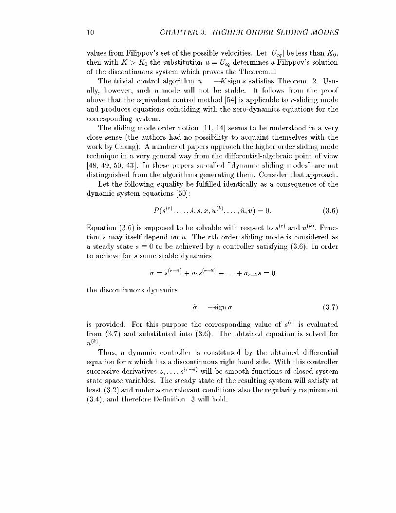
The trivial control algorithm u = �K sign s satis�es Theorem 2. Usu-ally, however, such a mode will not be stable. It follows from the proofabove that the equivalent control method [54] is applicable to r-sliding modeand produces equations coinciding with the zero-dynamics equations for thecorresponding system.

The sliding mode order notion [11, 14] seems to be understood in a veryclose sense (the authors had no possibility to acquaint themselves with thework by Chang). A number of papers approach the higher order sliding modetechnique in a very general way from the di�erential-algebraic point of view[48, 49, 50, 43]. In these papers so-called "dynamic sliding modes" are notdistinguished from the algorithms generating them. Consider that approach.

Let the following equality be ful�lled identically as a consequence of thedynamic system equations [50]:

P (s(r); : : : ; _s; s; x; u(k); : : : ; _u; u) = 0: (3.6)

Equation (3.6) is supposed to be solvable with respect to s(r) and u(k). Func-tion s may itself depend on u. The rth order sliding mode is considered asa steady state s � 0 to be achieved by a controller satisfying (3.6). In orderto achieve for s some stable dynamics

� = s(r�1) + a1s(r�2) + : : :+ ar�1s = 0

the discontinuous dynamics

_� = �sign � (3.7)

is provided. For this purpose the corresponding value of s(r) is evaluatedfrom (3.7) and substituted into (3.6). The obtained equation is solved foru(k).

Thus, a dynamic controller is constituted by the obtained di�erentialequation for u which has a discontinuous right hand side. With this controllersuccessive derivatives s; : : : ; s(r�1) will be smooth functions of closed systemstate space variables. The steady state of the resulting system will satisfy atleast (3.2) and under some relevant conditions also the regularity requirement(3.4), and therefore De�nition 3 will hold.

3.3. HIGHER ORDER SLIDING MODES IN CONTROL SYSTEMS 11

Hence, it may be said that the relation between our approach and theapproach by Sira-Ram��rez is a classical relation between geometric and alge-braic approaches in mathematics. Note that there are two di�erent slidingmodes in system (3.6), (3.7): a standard sliding mode of the �rst order whichis kept on the manifold � = 0, and an asymptotically stable r-sliding modewith respect to the constraint s = 0 which is kept in the points of the r-slidingmanifold s = _s = �s = : : : = s(r�1) = 0.

3.3.2 Real sliding and �nite time convergence

Recall that the objective is synthesis of such a control u that the constraints(t; x) = 0 holds. The quality of the control design is closely related tothe sliding accuracy. In reality, no approaches to this design problem mayprovide for ideal keeping of the prescribed constraint. Therefore, there is aneed to introduce some means in order to provide a capability for comparisonof di�erent controllers.

Any ideal sliding mode should be understood as a limit of motions whenswitching imperfections vanish and the switching frequency tends to in�nity(Filippov [21, 22]). Let " be some measure of these switching imperfections.Then sliding precision of any sliding mode technique may be featured by asliding precision asymptotics with "! 0 [35]:

De�nition 5 Let (t; x(t; ")) be a family of trajectories, indexed by " 2 R�,with common initial condition (t0; x(t0)), and let t � t0 (or t 2 [t0; T ]).Assume that there exists t1 � t0 (or t1 2 [t0; T ]) such that on every segment[t0; t00], where t0 � t1, (or on [t1; T ]) the function s(t; x(t; ")) tends uniformlyto zero with " tending to zero. In that case we call such a family a real-slidingfamily on the constraint s = 0. We call the motion on the interval [t0; t1] atransient process, and the motion on the interval [t1;1) (or [t1; T ]) a steadystate process.

De�nition 6 A control algorithm, dependent on a parameter " 2 R�, iscalled a real-sliding algorithm on the constraint s = 0 if, with "! 0, it formsa real-sliding family for any initial condition.

De�nition 7 Let (") be a real-valued function such that (")! 0 as "! 0.A real-sliding algorithm on the constraint s = 0 is said to be of order r (r > 0)with respect to (") if for any compact set of initial conditions and for any


time interval [T1; T2] there exists a constant C, such that the steady stateprocess for t 2 [T1; T2] satis�es

js(t; x(t; "))j � Cj (")jr:

In the particular case when (") is the smallest time interval of controlsmoothness, the words "with respect to " may be omitted. This is the casewhen real sliding appears as a result of switching discretization.

As follows from [35], with the r-sliding regularity condition satis�ed, inorder to get the rth order of real sliding with discrete switching it is nec-essary to get at least the rth order in ideal sliding (provided by in�niteswitching frequency). Thus, the real sliding order does not exceed the corre-sponding sliding mode order. The standard sliding modes provide, therefore,for the �rst order real sliding only. The second order of real sliding wasreally achieved by discrete switching modi�cations of the second order slid-ing algorithms [34, 16, 17, 18, 19, 35]. Any arbitrary order of real slidingcan be achieved by discretization of the same order sliding algorithms from[38, 39, 41]( see section 3.7).

Real sliding may also be achieved in a way di�erent from the discreteswitching realization of sliding mode. For example, high gain feedback sys-tems [47] constitute real sliding algorithms of the �rst order with respect tok�1, where k is a large gain. A special discrete-switching algorithm providingfor the second order real sliding were constructed in [52], another example ofa second order real sliding controller is the drift algorithm [18, 35]. A thirdorder real-sliding controller exploiting only measurements of s was recentlypresented [7].

It is true that in practice the �nal sliding accuracy is always achievedin �nite time. Nevertheless, besides the pure theoretical interest there arealso some practical reasons to search for sliding modes attracting in �nitetime. Consider a system with an r-sliding mode. Assume that with minimalswitching interval � the maximal r-th order of real sliding is provided. Thatmeans that the corresponding sliding precision jsj � � r is kept, if the r-thorder sliding condition holds at the initial moment. Suppose that the r-sliding mode in the continuous switching system is asymptotically stable anddoes not attract the trajectories in �nite time. It is reasonable to concludein that case that with � ! 0 the transient process time for �xed general caseinitial conditions will tend to in�nity. If, for example, the sliding mode wereexponentially stable, the transient process time would be proportional to

3.4. HIGHER ORDER SLIDING STABILITY IN RELAY SYSTEMS 13

r ln(��1). Therefore, it is impossible to observe such an accuracy in practice,if the sliding mode is only asymptotically stable. At the same time, thetime of the transient process will not change drastically if it was �nite fromthe very beginning. It has to be mentioned, also, that the authors are notaware of a case when a higher real-sliding order is achieved with in�nite-timeconvergence.

3.4 Higher order sliding stability in relay sys-

tems

In this section we present classical results by Tsypkin [53] (published inRussian in 1956) and Anosov (1959) [1]. They investigated the stability ofrelay control systems of the form

_y1 = y2; : : : ; _yl�1 = yl;_yl =

Pnj=1 al;jyj + k sign y1;

_yi =Pn

j=1 ai;jyj; i = l + 1; : : : ; n(3.8)

where ai;j = const; k 6= 0; and y1 = y2 = : : : = yl = 0 is the lth order slidingset.

The main result is as follows:

� for stability of equilibrium point of relay control system (3.8) with sec-ond order sliding (l = 2) three main cases are singled out: exponentiallystable, stable and unstable;

� it is shown that the equilibrium point of the system (3.8) is alwaysunstable with l � 3. Consequently, all higher order sliding modesarriving in the relay control systems are unstable with order of slidingmore than 2.

Consider the ideas of the proof.

3.4.1 2-sliding stability in relay systems

Consider a simple example of a second order dynamic system

_y1 = y2; _y2 = ay1 + by2 + k sign y1: (3.9)


The 2-sliding set is given here by y1 = y2 = 0. At �rst, let k < 0: Considerthe Lyapunov function

E =y222� a

y212+ jkjjy1j � b

2y1y2: (3.10)

Function E is an energy integral of system (3.9). Computing the derivativeof function E achieve

_E =b

2y22 +

b

2jy1j(jkj � ajy1j � by2sign y1):

It is obvious that for some positive �1 � �2, �1 � �2

�1jy1j+ �1y22 � E � �2jy1j+ �2y

22:

Thus, the inequalities � 2E � _E � � 1E or 1E � _E � 2E hold for b < 0or b > 0 respectively, in a small vicinity of the origin with some 2 � 1 > 0.

Let now k > 0. It is easy to see in that case that trajectories cannotleave the set y1 > 0, y2 = _y1 > 0 if a � 0. The same is true with y1 < k=jajif a < 0. Starting with in�nitisimally small y1 > 0, y2 > 0, any trajectoryinevitably leaves some �xed origin vicinity.

It allows three main cases to be singled out for investigation of stabilityof system (3.9).

� Exponentially stable case. Under the conditions

b < 0; k < 0 (3.11)

the equilibrium point y1 = y2 = 0 is exponentially stable.

� Unstable case. Under the condition

k > 0 or b > 0

the equilibrium point y1 = y2 = 0 is unstable.

� Critical case.k � 0; b � 0; bk = 0:

With b = 0; k < 0 the equilibrium point y1 = y2 = 0 is stable.

It is easy to show that if the matrix A consisting of ai;j; i; j > 2 is Hurvitzand conditions a2;2 < 0; k < 0 are true, the equilibrium point of system (3.8)is exponentially stable.

3.5. SLIDING ORDER AND DYNAMIC ACTUATORS 15

3.4.2 Relay system instability with sliding order more

than 2

Let us illustrate the idea of the proof on an example of a simple third ordersystem

_y1 = y2; _y2 = y3; _y3 = a31y1 + a32y2 + a33y3 � k sign y1; k > 0: (3.12)

Consider the Lyapunov function1

V = y1y3 � 1

2y22:

Thus,_V = �kjy1j+ y1(a31y1 + a32y2 + a33y3);

and _V is negative at least in a small neighbourhood of origin (0; 0; 0): Thatmeans that the zero solution of system (3.12) is unstable.

On the other hand, in relay control systems with order of sliding morethan 2 a stable periodic solution can occur [46, 32].

3.5 Sliding order and dynamic actuators

Let the constraint be given by the equality of some constraint function s tozero and let the sliding mode s � 0 be provided by a relay control. Takinginto account an actuator conducting a control signal to the process controlled,we achieve more complicated dynamics. In that case the relay control uenters the actuator and continuous output variables of the actuator z aretransmitted to the plant input ( Fig. 3.2). As a result discontinuous switchingis hidden now in the higher derivatives of the constraint function [55, 23, 24,25, 26, 27, 9].

3.5.1 Stability of 2-sliding modes in systems with fast

actuators

Condition (3.11) is used in [25, 26, 27, 9] for analysis of sliding mode systemswith fast dynamic actuators. Here is a simple outline of these reasonings. Oneof the actuator output variables is formally replaced by _s after application

1this function was suggested by V.I. Utkin in private communications


Plant

Relay Controller

Actuator

�s

6u

-z

Figure 3.2: Control system with actuator

of some coordinate transformation. Let the system under consideration berewritten in the following form:

� _z = Az +B� +D1x;� _� = Cz + b� +D2x+ k sign s;_s = �;_x = F (z; �; s; x);

(3.13)

where z 2 Rm; x 2 Rn; �; s 2 R.With (3.11) ful�lled and ReSpecA < 0 system (3.13) has an exponentially

stable integral manifold of slow motions being a subset of the second ordersliding manifold and given by the equations

z = H(�; x) = �A�1D1x+O(�); s = � = 0:

Function H may be evaluated with any desired precision with respect to thesmall parameter � .

Therefore, according to [25, 26, 27, 9] under the conditions

ReSpecA < 0; b < 0; k < 0 (3.14)

the motions in such a system with a fast actuator of relative degree 1 consist offast oscillations, vanishing exponentially, and slow motions on a submanifoldof the second order sliding manifold.

Thus, if conditions (3.14) of chattering absence hold, the presence of afast actuator of relative degree 1 does not lead to chattering in sliding modecontrol systems.


Remark

The stability of the fast actuator and of the second order sliding mode in(3.13) still does not guarantee absence of chattering if dim z > 0 and @F

@z 6= 0,for in that case fast oscillations may still remain in the 2-sliding mode itself.Indeed, the stability of a fast actuator corresponds to the stability of the fastactuator matrix

Re Spec

�A BC b

�< 0:

Consider the system

� _z1 = z1 + z2 + � +D1x;� _z2 = 2z2 + z3 +D2x;� _� = 24z1 � 60z2 � 9� +D3x+ k sign s;_s = �;_x = F (z1; z2; �; s; x);

where z1; z2; �; s are scalars. It is easy to check that the spectrum of thematrix is f�1;�2;�3g and condition (3.11) holds for this system. On theother hand the motions in the second order sliding mode are described bythe system

� _z1 = z1 + z2 +D1x;� _z2 = 2z2 +D2x;_x = F (z1; z2; 0; 0; x):

The fast motions in this system are unstable and the absence of chatteringin the original system cannot be guaranteed.

Example

Without loss of generality we illustrate the approach by some simple exam-ples. Consider, for instance, sliding mode usage for the tracking purpose. Letthe process be described by the equation _x = u; x; u 2 R, and the slidingvariable be

s = x� f(t); f : R! R,

so that the problem is to track a signal f(t) given in real time, wherejf j; j _f j; j �f j < 0:5. Only values of x; f; u are available.

The problem is successfully solved by the controller u = �sign s, keepings = 0 in a 1-sliding mode. In practice, however, there is always some actuator


between the plant and the controller, which inserts some additional dynamicsand removes the discontinuity from the real system. With respect to Fig. 3.2let the system be described by the equation

_x = v;

where v 2 R is an output of some dynamic actuator. Assume that theactuator has some fast �rst order dynamics. For example

� _v = u� v

The input u of the actuator is the relay control

u = �sign s:where � is a small positive number. The second order sliding manifold S2 isgiven here by the equations

s = x� f(t) = 0; _s = v � _f(t) = 0:

The equality

�s =1

�(u� v)� �f(t)

shows that the relative degree here equals 2 and, according to Theorem 2, a2-sliding mode exists, provided � < 1. The motion in this mode is describedby the equivalent control method or by zero-dynamics, which is the same:from s = _s = �s = 0 achieve u = � �f(t) + v, v = _f(t) and therefore

x = f(t); v = _f(t); u = � �f(t) + v:

It is easy to prove that the 2-sliding mode is stable here with � small enough.Note that the latter equality describes the equivalent control [54, 55] and iskept actually only in the average, while the former two are kept accuratelyin the 2-sliding mode.

Let

f(t) = 0:08 sin t+ 0:12 cos 0:3t ; x(0) = 0; v(0) = 0 :

The plots of x(t) and f(t) with � = 0:2 are shown in Fig. 3.3, whereas theplot of v(t) is demonstrated in Fig. 3.4.


0.000000E+00 5.988000-6.961547E-02

1.897384E-01

0 `̀̀````

`

`

````````````````

````````````````````````````````

`

```̀`̀̀`````

`

`

`

```̀`̀̀`````

`

`

`

```̀̀`̀````̀`̀̀``````̀`̀̀``̀`̀̀```̀`̀̀`̀`̀̀``̀̀ `̀`̀̀ `̀

`̀̀`̀̀`̀̀`̀̀ `̀̀`̀̀`̀̀`̀̀ `̀`̀̀`̀̀`̀̀`̀̀ `̀̀

`̀̀`̀̀`̀̀`̀̀`̀̀`̀̀`̀`̀̀`̀̀`̀`̀̀`̀`̀`̀̀`̀`̀`̀`̀`̀`̀`̀`̀`̀`̀`̀`̀`̀`̀`̀`̀`̀`̀`̀`̀`̀`̀`̀`̀`̀`̀`̀`̀`̀`̀`̀`̀`̀`̀`̀`̀`̀`̀`̀`̀`̀`̀`̀`̀`̀`̀`̀`̀`̀`̀`̀`̀`̀`̀`̀`̀`̀`̀`̀`̀`̀`̀`̀`̀`̀`̀`̀`̀`̀`̀`̀`̀`̀`̀`̀`̀`̀`̀`̀`̀̀`̀`̀̀`̀̀`̀̀`̀̀`̀̀`̀̀`̀̀`̀̀`̀̀ `̀̀

`̀̀`̀̀`̀̀ `̀̀`̀̀`̀̀`̀̀ `̀̀`̀̀`̀̀ `̀̀`̀̀`̀̀`̀̀ `̀̀`̀̀`̀̀`̀̀ `̀̀`̀̀`̀̀`̀̀`̀̀`̀̀`̀̀

`̀̀ `̀̀`̀̀`̀̀`̀̀

`̀̀`̀̀`̀̀`̀̀

`̀̀`̀̀`̀̀ `̀̀

`̀`̀`̀`̀`̀`̀`̀`̀`̀`̀`̀`̀̀`̀`̀̀`̀̀`̀̀`̀`̀̀`̀̀`̀̀`̀̀`̀̀`̀̀`̀̀`̀̀`̀̀`̀̀`̀̀ `̀̀

`̀̀`̀̀`̀̀ `̀̀

`̀̀`̀̀`̀̀ `̀̀`̀̀

`̀̀`̀̀ `̀̀`̀̀`̀̀`̀̀ `̀̀`̀̀`̀̀`̀̀ `̀̀`̀̀`̀̀ `̀̀`̀̀`̀̀`̀̀ `̀̀`̀̀`̀̀`̀̀ `̀̀

`̀̀`̀̀`̀̀`̀̀`̀̀`̀̀`̀`̀`̀`̀`̀`̀`̀`̀`̀`̀`̀`̀`̀`̀`̀`̀`̀`̀`̀`̀`̀`̀`̀`̀`̀`̀`̀`̀`̀`̀`̀`̀`̀`̀`̀`̀`̀`̀`̀`̀`̀`̀`̀`̀`̀`̀`̀`̀`̀`̀`̀`̀`̀`̀`̀`̀`̀`̀`̀`̀`̀`̀`̀`̀`̀`̀`̀`̀`̀`̀`̀`̀`̀`̀`̀`̀`̀`̀`̀`̀`̀`̀`̀`̀`̀̀`̀̀`̀̀`̀̀`̀̀`̀̀`̀̀`̀̀`̀̀`̀̀

`̀̀`̀̀`̀̀`̀̀ `̀̀`̀̀`̀̀`̀̀ `̀̀`̀̀`̀̀ `̀̀`̀̀`̀̀`̀̀ `̀̀`̀̀`̀̀`̀̀ `̀̀`̀̀`̀̀`̀̀`̀̀`̀̀`̀̀

`̀̀ `̀̀`̀̀`̀̀

`̀̀ `̀̀`̀̀`̀̀`̀̀ `̀̀

`̀̀`̀̀`̀̀

Figure 3.3: Asymptotically stable second order sliding mode in a system witha fast actuator. Tracking: x(t) and f(t).

0.000000E+00 5.988000-4.040195E-01

7.630808E-01

0 ````````````````````````````````

``````````````

`

`

`

`

````̀

`````````````````````````````````````````````````````````````````````````````````````````````````````````````````````````````````````````````````````````````````````````````````````````````````````````

``````````````````````````````````````````````````````````````````````````

``````````````````````````````````````````````````````````````````````````````````````````````````````````````̀`````````````

`````````````̀````````````````````````````````

````````

````````

```````̀````

`̀

````̀

```

`̀````̀`

``̀

`

`̀`

``̀

``̀```̀

``̀``````̀``̀̀`̀̀`̀̀`̀̀`

`̀̀`̀̀`̀̀`̀̀ `̀

`̀`̀̀ `̀̀`̀̀`̀`̀̀`̀̀ `̀̀`̀̀`̀̀`̀̀ `̀̀`̀̀`̀̀`̀̀ `̀̀`̀̀`̀̀`̀̀ `̀̀`̀̀`̀̀`̀̀ `̀̀`̀̀`̀̀ `̀̀`̀̀`̀̀

`̀̀ `̀̀`̀̀`̀̀`̀̀ `̀̀`̀̀`̀̀`̀̀ `̀̀`̀̀

`̀̀`̀̀ `̀̀`̀̀`̀̀ `̀̀`̀̀`̀̀

`̀̀ `̀̀`̀̀`̀̀`̀̀ `̀̀`̀̀

`̀̀`̀̀ `̀̀`̀̀`̀̀`̀̀ `̀̀

`̀̀`̀̀`̀̀ `̀̀`̀̀`̀̀ `̀̀

`̀̀`̀̀`̀̀`̀̀`̀̀`̀̀`̀̀

`̀̀`̀̀`̀̀`̀̀ `̀̀`̀̀`̀̀

`̀̀ `̀̀`̀̀`̀̀`̀̀`̀̀`̀̀`̀̀`̀̀ `̀̀`̀̀

`̀̀ `̀̀

Figure 3.4: Asymptotically stable second order sliding mode in a system witha fast actuator: actuator output v(t).


3.5.2 Systems with fast actuators of relative degree 3

and higher

The equilibrium point of any relay system with relative degree � 3 is al-ways unstable [1, 53] (section 3.4.2). That leads to an important conclusion:even being stable, higher order actuators do not suppress chattering in theclosed-loop relay systems. For investigation of chattering phenomena in suchsystems the averaging technique was used [25, 29]. Higher-order actuatorsmay give rise to high-frequency periodic solutions. The general model ofsliding mode control systems with fast actuators has the form [10]

_x = h(x; s; �; z; u(s)); _s = �;

� _� = g2(x; s; �; z); � _z = g1(x; s; �; z; u(s)); (3.15)

where z 2 Rm; �; s 2 R; x 2 X � Rn, u(s) = signs, and g1; g2; h are smoothfunctions of their arguments. Variables s; x may be considered as the statecoordinates of the plant, �; z being the fast-actuator coordinates, and � beingthe actuator time constant.

Suppose that following conditions are true:1. The fast-motion system

ds

d�= �;

d�

d�= g2(x; 0; �; z);

dz

d�= g1(x; 0; �; z; u(s)); (3.16)

has a T (x)-periodic solution (s0(� ; x); �0(�; x); z0(� ; x)) for any x 2 X. Sys-tem (3.16) generates a point mapping (x; �; z) of the switching surfaces = 0 into itself which has a �xed point (��(x); z�(x)), (x; ��(x); z�(x)) =(��(x); z�(x)): Moreover, the Frechet derivative of (x; �; z) with respect tovariables (�; z) calculated at (��(x); z�(x)) is a contractive matrix for anyx 2 �X .

2. The averaged system

_x = �h(x) =1

T (x)

Z T (x)

0h(x; 0; �0(� ; x); z0(�; x); u(s0(� ; x)))d� (3.17)

has an unique equilibrium point x = x0: This equilibrium point is exponen-tially stable.

Theorem 3 [29]. Under conditions 1,2 system (3.15) has an isolated or-bitally asymptotically stable periodic solution with the period �(T (x0)+O(�))near the closed curve

(x0; �s0(t=�; x0); �0(t=�; x0); z0(t=�; x0)):


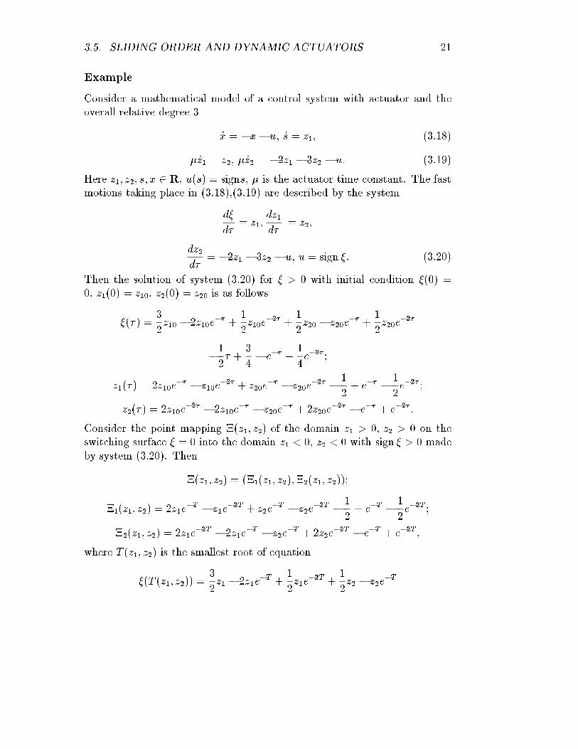
Example

Consider a mathematical model of a control system with actuator and theoverall relative degree 3

_x = �x� u; _s = z1; (3.18)

� _z1 = z2; � _z2 = �2z1 � 3z2 � u: (3.19)

Here z1; z2; s; x 2 R, u(s) = signs, � is the actuator time constant. The fastmotions taking place in (3.18),(3.19) are described by the system

d�

d�= z1;

dz1d�

= z2;

dz2d�

= �2z1 � 3z2 � u; u = sign �: (3.20)

Then the solution of system (3.20) for � > 0 with initial condition �(0) =0; z1(0) = z10; z2(0) = z20 is as follows

�(� ) =3

2z10 � 2z10e

�� +1

2z10e

�2� +1

2z20 � z20e

�� +1

2z20e

�2�

�1

2� +

3

4� e�� +

1

4e�2� ;

z1(�) = 2z10e�� z10e

�2� + z20e�� z20e

�2� � 1

2+ e�� 1

2e�2� ;

z2(� ) = 2z10e�2� � 2z10e

�� z20e�� + 2z20e

�2� � e�� + e�2� :

Consider the point mapping �(z1; z2) of the domain z1 > 0; z2 > 0 on theswitching surface � = 0 into the domain z1 < 0; z2 < 0 with sign � > 0 madeby system (3.20). Then

�(z1; z2) = (�1(z1; z2);�2(z1; z2));

�1(z1; z2) = 2z1e�T � z1e

�2T + z2e�T � z2e

�2T � 1

2+ e�T � 1

2e�2T ;

�2(z1; z2) = 2z1e�2T � 2z1e

�T � z2e�T + 2z2e

�2T � e�T + e�2T ;

where T (z1; z2) is the smallest root of equation

�(T (z1; z2)) =3

2z1 � 2z1e

�T +1

2z1e

�2T +1

2z2 � z2e

�T


+1

2z2e

�2T � 1

2T +

3

4� e�T +

1

4e�2T = 0:

System (3.20) is symmetric with respect to the point � = z1 = z2 = 0:Thus, the initial condition (0; z�1; z

�2) and the semi-period T � = T (z�1; z

�2) for

the periodic solution of (3.20) are determined by the equations �(z�1; z�2) =

�(z�1; z�2); �(T (z�1; z�2)) = 0 and consequently

3

2z�1 � 2z�1e

�T � +1

2z�1e

�2T � +1

2z�2 � z�2e

�T � +1

2z�2e

�2T �

�1

2T � +

3

4� e�T

�

+1

4e�2T

�

= 0:

2z�1e�T � � z�1e

�2T � + z�2e�T � � z�2e

�2T � � 1

2+ e�T � 1

2e�2T = �z�1;

2z�1e�2T � � 2z�1e

�T � � z�2e�T � + 2z�2e

�2T � � e�T�

+ e�2T�

= �z�2; (3.21)

Expressing z�1; z�2 from the latter two equations of (3.21), achieve

T �(eT�

+ e3T�

+ 1 + e2T�

)� 5eT� � 3e3T

�

+ 3 + 5e2T�

= 0: (3.22)

Equations (3.22) and (3.21) have positive solution

T � � 2:2755; z�1 � 0:3241; z�2 � 0:1654;

corresponding to the existence of a 2T �-periodic solution in system (3.20).Thus

(@T

@z1;@T

@z2) =

(�32 � 2e�T + 1

2e�2T

(2z1 + z2 + 1)e�T � (z1 + z2 +12)e

�2T � 12

;

�12 � e�T + 1

2e�2T

(2z1 + z2 + 1)e�T � (z1 + z2 +12)e

�2T � 12

)

and

@�1

@z1= 2e�T � e�2T + [e�2T(2z1 + 2z2 + 1)� e�T (2z1 + z2 + 1)]

@T

@z1;

@�1

@z2= e�T � e�2T + [e�2T (2z1 + 2z2 + 1)� e�T (2z1 + z2 + 1)]

@T

@z2;

3.6. 2-SLIDING CONTROLLERS 23

@�2

@z1= 2e�2T � 2e�T � [(e�T (2z1 + z2 + 1) � 2e�2T (2z1 + 2z2 + 1)]

@T

@z1;

@�2

@z2= 2e�2T � e�T � [(e�T (2z1 + z2 + 1)� 2e�2T (2z1 + 2z2 + 1)]

@T

@z2:

Calculating the value of Frechet derivative @�@z at (z�1; z

�2), using the found

value of T �, achieve

@�

@z(z�1; z

�2) = J =

� �0:4686 �0:11330:3954 0:0979

�:

The eigenvalues of matrix J are �0:3736 and 0:0029: That implies existenceand asymptotic stability of the periodic solution of (3.20). The averagedequation for system (3.18),(3.19) is

_x = �x;and it has the asymptotically stable equilibrium point x = 0. Hence, system(3.18),(3.19) has an orbitally asymptotically stable periodic solution whichlies in the O(�)-neighbourhood of the switching surface.

3.6 2-sliding controllers

We follow here [36, 35, 6].

3.6.1 2-sliding dynamics

Return to the system

_x = f(t; x; u); s = s(t; x) 2 R; u = U(t; x) 2 R; (3.23)

where x 2 Rn, t is time, u is control, and f; s are smooth functions. Thecontrol task is to keep output s � 0.

Di�erentiating successively the output variable s achieve functions _s; �s; :::Depending on the relative degree [31] of the system di�erent cases should beconsidered

a) relative degree r = 1, i.e., @@u _s 6= 0;

b) relative degree r � 2, i.e., @@us

(i) = 0 (i = 1; 2; : : : ; r � 1), @@us

(r) 6= 0.


In case a) the classical VSS approach solves the control problem by meansof 1{sliding mode control, nevertheless 2{sliding mode control can also beused in order to avoid chattering. For that purpose u is to become an outputof some �rst order dynamic system [35]. For example, the time derivative ofthe plant control _u(t) may be considered as the actual control variable. Adiscontinuous control _u steers the sliding variable s to zero, keeping s = 0 ina 2{sliding mode, so that the plant control u is continuous and the chatteringis avoided [35, 5]. In case b) the p{sliding mode approach, with p � r, is thecontrol technique of choice.

Chattering avoidance: the generalized constraint ful�llment prob-lem

When considering classical VSS the control variable u(t) is a feedback-designedrelay output. The most direct application of 2{sliding mode control is thatof attaining sliding motion on the sliding manifold by means of a continu-ous bounded input u(t) being a continuous output of a suitable �rst{orderdynamical system driven by a proper discontinuous signal. Such �rst{orderdynamics can be either inherent to the control device or specially introducedfor chattering elimination purposes.

Assume that f and s are respectively C1 and C2 functions, and that theonly available current information consists of the current values of t, u(t),s(t; x) and, possibly, of the sign of the time derivative of s. Di�erentiatingthe sliding variable s twice, the following relations are derived:

_s =@

@ts(t; x) +

@

@xs(t; x)f(t; x; u); (3.24)

�s(t) =@

@t_s(t; x; u) +

@

@x_s(t; x; u)f(t; x; u) +

@

@u_s(t; x; u) _u(t): (3.25)

The control goal for a 2{sliding mode controller is that of steering s tozero in �nite time by means of control u(t) continuously dependent on time.In order to state a rigorous control problem the following conditions areassumed:

1) Control values belong to the set U = fu : juj � UMg, where UM > 1 isa real constant; furthermore the solution of the system is well de�nedfor all t, provided u(t) is continuous and 8t u(t) 2 U .


2) There exists u1 2 (0; 1) such that for any continuous function u(t) withju(t)j > u1, there is t1, such that s(t)u(t) > 0 for each t > t1. Hence,the control u(t) = �sign(s(t0)), where t0 is the initial value of time,provides hitting the manifold s = 0 in �nite time.

3) Let _s(t; x; u) be the total time derivative of the sliding variable s(t; x).There are positive constants s0, u0 < 1, �m, �M such that if js(t; x)j <s0 then

0 < �m � @

@u_s(t; x; u) � �M ;8u 2 U ; x 2 X (3.26)

and the inequality juj > u0 entails _su > 0.

4) There is a positive constant � such that within the region jsj < s0 thefollowing inequality holds 8t; x 2 X ; u 2 U�� @@t _s(t; x; u) + @

@x_s(t; x; u)f(t; x; u)

�� (3.27)

The above condition 2 means that starting from any point of the statespace it is possible to de�ne a proper control u(t) steering the sliding variablewithin a set such that the boundedness conditions on the sliding dynamicsde�ned by conditions 3 and 4 are satis�ed. In particular they state that thesecond time derivative of the sliding variable s, evaluated with �xed valuesof the control u, is uniformly bounded in a bounded domain.

It follows from the theorem on implicit function that there is a functionueq(t; x) which can be considered as equivalent control [55] satisfying theequation _s = 0. Once s = 0 is attained, the control u = ueq(t; x) wouldprovide for the exact constraint ful�llment. Conditions 3 and 4 mean thatjsj < s0 implies jueqj < u0 < 1, and that the velocity of the ueq changing isbounded. This provides for a possibility to approximate ueq by a Lipschitziancontrol.

The unit upper bound for u0 and u1 is actually a scaling factor. Notealso that linear dependence on control u is not required here. The usualform of the uncertain systems dealt with by the VSS theory, i.e., systemsa�ne in u and possibly in x, are a special case of the considered systemand the corresponding constraint ful�llment problem may be reduced to theconsidered one [35, 20].

Relative degree two. In case of relative degree two the control problemstatement could be derived from the above by considering the variable u as a


state variable and _u as the actual control. Indeed, let the controlled systembe

f(t; x; u) = a(t; x) + b(t; x)u(t); (3.28)

where a : Rn+1 ! Rn and b : Rn+1 ! Rn are su�ciently smooth uncertainvector functions, [ @@xs(t; x)]b(t; x) � 0. Calculating achieve that

�s = '(t; x) + (t; x)u: (3.29)

It is assumed that j'j � �; 0 < �m � � �M ;� > 0.Thus in a small vicinity of the manifold s = 0 the system is described by

(3.28), (3.29) if the relative degree is 2 or by (3.23) and

�s = '(t; x) + (t; x) _u; (3.30)

if the relative degree is 1.

3.6.2 Twisting algorithm

Let relative degree be 1. Consider local coordinates y1 = s and y2 = _s,then after a proper initialization phase, the second order sliding mode controlproblem is equivalent to the �nite time stabilization problem for the uncertainsecond order system with j'j � �; 0 < �m � � �M ;� > 0.�

_y1 = y2_y2 = '(t; x) + (t; x) _u

(3.31)

with y2(t) immeasurable but with a possibly known sign, and '(t; x) and (t; x) uncertain functions with

� > 0; j'j � �; 0 < �m � � �M : (3.32)

Being historically the �rst known 2-sliding controller [34], that algorithmfeatures twisting around the origin of the 2{sliding plane y1Oy2 (Fig.3.5).The trajectories perform an in�nite number of rotations while converging in�nite time to the origin. The vibration magnitudes along the axes as well asthe rotation times decrease in geometric progression. The control derivativevalue commutes at each axis crossing, which requires availability of the signof the sliding-variable time-derivative y2.


Figure 3.5: Twisting algorithm phase trajectory

The control algorithm is de�ned by the following control law [34, 35, 17,20], in which the condition on juj provides for juj � 1:

_u(t) =

8<:�u if juj > 1;�Vmsign(y1) if y1y2 � 0; juj � 1;�VMsign(y1) if y1y2 > 0; juj � 1:

(3.33)

The corresponding su�cient conditions for the �nite time convergence to thesliding manifold are [35]

VM > VmVm > 4�M

s0Vm > �

�m�mVM � � > �MVm + �:

(3.34)

The similar controller

u(t) =

� �Vmsign(y1) if y1y2 � 0�VM sign(y1) if y1y2 > 0

is to be used in order to control system (3.28) when the relative degree is 2.By taking into account the di�erent limit trajectories arising from the

uncertain dynamics of (3.29) and evaluating time intervals between successivecrossings of the abscissa axis, it is possible to de�ne the following upper bound


for the convergence time [6]

ttw1 � tM1+�tw

1

1 � �tw

qjy1M1

j: (3.35)

Here y1M1is the value of the y1 variable at the �rst abscissa crossing in the

y1Oy2 plane, tM1is the corresponding time instant and

�tw =p2 �mVM+�MVm(�mVM��)

p�MVm+�

�tw =q

�MVm+��mVM�� :

In practice when y2 is immeasurable, its sign can be estimated by the signof the �rst di�erence of the available sliding variable y1 in a time interval � ,i.e., sign(y2(t)) is estimated by sign(y1(t) � y1(t � � )). In that case the 2{sliding precision with respect to the measurement time interval is provided,and the size of the boundary layer of the sliding manifold is � � O(� 2) [35].Recall that it is the best possible accuracy asymptotics with discontinuous_y2 = �s.

3.6.3 Sub{optimal algorithm

That 2{sliding controller was developed as a sub{optimal feedback imple-mentation of a classical time-optimal control for a double integrator. Let therelative degree be 2. The auxiliary system is

�_y1 = y2_y2 = '(t; x) + (t; x)u:

(3.36)

The trajectories on the y1Oy2 plane are con�ned within limit parabolic arcswhich include the origin, so that both twisting and leaping (when y1 and y2 donot change sign) behaviors are possible (Fig.3.6). Also here the coordinatesof the trajectory intersections with axis y1 decrease in geometric progression.After an initialization phase the algorithm is de�ned by the following controllaw [4, 5, 6]:

v(t) = ��(t)VMsign(y1(t)� 12y1M );

�(t) =

�� if [y1(t)� 1

2y1M ][y1M � y1(t)] > 01 if [y1(t)� 1

2y1M ][y1M � y1(t)] � 0;

(3.37)


Figure 3.6: Sub{Optimal algorithm phase trajectories

where y1M is the latter singular value of the function y1(t), i.e. the lattervalue corresponding to the zero value of y2 = _y1. The corresponding su�-cient conditions for the �nite-time convergence to the sliding manifold are asfollows [4]:

�� 2 (0; 1] \ (0; 3�m�M);

VM > max�

��m

; 4�3�m��M

�:

(3.38)

Also in that case an upper bound for the convergence time can be deter-mined [4]

topt1 � tM1+�opt

1

1 � �opt

qjy1M1

j: (3.39)

Here y1M1and tM1

are de�ned as for the twisting algorithm, and

�opt =(�m+��M)VM

(�mVM��)p��MVM+�

;

�opt =q

(��M��m)VM+2�2(�mVM��) :

The e�ectiveness of the above algorithm was extended to larger classes ofuncertain systems [6]. It was proved [5] that in case of unit gain function thecontrol law (3.37) can be simpli�ed by setting � = 1 and choosing VM > 2�.

The sub{optimal algorithm requires some device in order to detect thesingular values of the available sliding variable y1 = s. In the most practicalcase y1M can be estimated by checking the sign of the quantity D(t) =[y1(t� � )� y1(t)] y1(t) in which �

2 is the estimation delay. In that case thecontrol amplitude VM has to belong to an interval instead of a half-line:


VM 2�max

��

��m; VM1

(� ; y1M )

�; VM2

(� ; y1M )

�(3.40)

Here VM1< VM2

are the solutions of the second order algebraic equation�(3�m � ��M )

VMi

�� 4

�y1M��2

� VMi

8�[�m + �M (2 � ��)]

��M

VMi

�+ 1

�= 0

In the case of approximated evaluation of y1M the second order real slidingmode is achieved, and the size of the boundary layer of the sliding manifoldis � � O(� 2). It can be minimized by choosing VM as follows [6]:

VM =4�

3�m � ��M

"1 +

r1 +

3�m � ��M4�M

#

An extension of the sub{optimal 2{sliding controller to a class of sampleddata systems such that the gain function in (3.29 ) is constant, i.e., (�) = 1,was recently presented [6].

3.6.4 Super{twisting algorithm

That algorithm has been developed to control systems with relative degreeone in order to avoid chattering in VSC. Also in that case the trajectories onthe 2{sliding plane are characterized by twisting around the origin (Fig.3.7),but the continuous control law u(t) is constituted by two terms. The �rstis de�ned by means of its discontinuous time derivative, while the other is acontinuous function of the available sliding variable.

The control algorithm is de�ned by the following control law [35]:

u(t) = u1(t) + u2(t)

_u1(t) =

� �u if juj > 1�W sign(y1) if juj � 1

u2(t) =

� ��js0j�sign(y1) if jy1j > s0��jy1j�sign(y1) if jy1j � s0

(3.41)

and the corresponding su�cient conditions for the �nite time convergence tothe sliding manifold are [35]

W > ��m

�2 � 4��2m

�M(W+�)�m(W��)

0 < � � 0:5

(3.42)


Figure 3.7: Super{Twisting algorithm phase trajectory

That controller may be simpli�ed when controlled systems (3.28) arelinearly dependent on control, u does not need to be bounded and s0 =1:

u = ��jsj�sign(y1) + u1;_u1 = �W sign(y1):

The super-twisting algorithm does not need any information on the timederivative of the sliding variable. An exponentially stable 2{sliding modearrives if the control law (3.41) with � = 1 is used. The choice � = 0:5assures that the maximal possible for 2{sliding realization real-sliding order2 is achieved. Being extremely robust, that controller is successfully used forreal-time robust exact di�erentiation [37] ( see further).

3.6.5 Drift algorithm

The idea of the controller is to steer the trajectory to the 2-sliding modes = 0 while keeping _s relatively small, i.e. to cause "drift" towards the originalong axis y1. When using the drift algorithm, the phase trajectories on the2-sliding plane are characterized by loops with constant sign of the slidingvariable y1 (Fig.3.8). That controller intentionally yields real 2-sliding anduses sampled values of the available signal y1 with sampling period � . Thecontrol algorithm is de�ned by the following control law [35, 16, 18] (relative


Figure 3.8: Drift algorithm phase trajectories

degree is 1):

_u =

8<:�u if juj > 1�Vmsign(�y1i) if y1�y1i � 0; juj � 1�VMsign(�y1i) if y1�y1i > 0; juj � 1

(3.43)

where Vm and VM are proper positive constants such that Vm < VM andVMVm

is su�ciently large, and �y1i = y1(ti) � y1(ti � � ), t 2 [ti; ti+1). Thecorresponding su�cient conditions for the convergence to the sliding manifoldare rather cumbersome [18] and are omitted here for the sake of simplicity.Also here a similar controller corresponds to relative degree 2:

_u =

� �Vmsign(�y1i) if y1�y1i � 0�VM sign(�y1i) if y1�y1i > 0

After substituting y2 for �y1i a �rst order sliding mode on y2 = 0 wouldbe achieved. That implies y1 = const, but since an arti�cial switching timedelay appears, we ensure a real sliding on y2 with most of time spent in theregion y1y2 < 0. Therefore, y1 ! 0. The accuracy of the real sliding ony2 = 0 is proportional to the sampling time interval � ; hence, the durationof the transient process is proportional to ��1.

Such an algorithm does not satisfy the de�nition of a real sliding algorithm(Section 3.3) requiring the convergence time to be uniformly bounded withrespect to � . Consider a variable sampling time � i+1[y1(ti)] = ti+1 � ti,i = 0; 1; 2; : : : with � = max(�M ;min(�m; �jy1(ti)j�)), where 0:5 � � � 1,�M > �m > 0, � > 0. Then with �, Vm

VMsu�ciently small and Vm su�ciently


large the drift algorithm constitutes a second order real sliding algorithmwith respect to � ! 0. That algorithm has no overshoot if the parametersare chosen properly [18].

3.6.6 Algorithm with a prescribed convergence law

That class of sliding controllers features the possibility of choosing a transientprocess trajectory: the switching of _u depends on a suitable function of s.

Figure 3.9: Phase trajectories for the algorithm with prescribed law of vari-ation of s

The general formulation of such a class of 2{sliding control algorithms isas follows :

_u =

� �u if juj > 1�VM sign(y2 � g(y1)) if juj � 1

(3.44)

Here VM is a positive constant and the continuous function g(y1) is smootheverywhere but in y1 = 0. A controller for the relative degree 2 is formed inan obvious way:

_u = �VM sign(y2 � g(y1)):

Function g must be chosen in such a way that all solutions of the equation_y1 = g(y1) vanish in �nite time and the function g0 � g be bounded. Forexample, the following function can be used

g(y1) = ��1jy1j�sign(y1); � > 0 ; 0:5 � � < 1:


The su�cient condition for the �nite time convergence to the slidingmanifold is de�ned by the following inequality

VM >� + sup(g0(y1)g(y1))

�m; (3.45)

and the convergence time depends on the function g [16, 35, 56].That algorithm needs y2 to be available, which is not always the case. The

substitution of the �rst di�erence of y1for y2 i.e. sign[�y1i � � ig(y1)] insteadof sign[y2 � g(y1)] (t 2 [ti; ti+1); � i = ti � ti�1), turns the algorithm into areal sliding algorithm. The real sliding order equals two if g(�) is chosen asin the above example with � = 0:5 [35].

Important remark. All the above-listed discretized 2-sliding controllers,except for the super-twisting one, are sensitive to the choice of the mea-surement interval � . Indeed, given any measurement error magnitude, anyinformation signi�cance of the �rst di�erence �y1i is eliminated with su�-ciently small � , and the algorithm convergence is disturbed. That problemwas shown to be solved [40] by a special feedback determinating � as a func-tion of the real-time measured value of y1. In particular, it was shown thatthe feedback � = max(�M ;min(�m; �jy1(ti)j�)), 0:5 � � � 1, �M > �m > 0,� > 0, makes the twisting controller robust with respect to measurementserrors. Moreover, the choice � = 1=2 is proved to be the best one. It providesfor keeping the second order real-sliding accuracy s = O(� 2) in the absenceof measurement errors and for sliding accuracy proportional to the maximalerror magnitude otherwise. Note that the super-twisting controller is robustdue to its own nature and does not need such auxiliary constructions.

3.6.7 Examples

Practical implementation of 2-sliding controllers is described in [42]. Contin-ue the example series 3.5.1, 3.5.2. The process is given by

_x = u; x; u 2 R; s = x� f(t); f : R! R;

so that the problem is to track a signal f(t) given in real time, wherejf j; j _f j; j �f j < 0:5. Only values of x; f; u are available. Following is theappropriate discretized twisting controller:

_u =

8<:�u(ti); ju(ti)j > 1;�5 sign s(ti); s(ti)�si > 0; ju(ti)j � 1;� sign s(ti); s(ti)�si � 0; ju(ti)j � 1:

3.7. ARBITRARY-ORDER SLIDING CONTROLLERS 35

0.000000E+00 5.988000-6.939553E-02

1.903470E-01

0 `̀̀`̀``̀`````````````

``

`

`

`

`

`

`

`

`````````````````````````````

`

````̀`̀̀`̀̀ `̀̀`̀

`̀`̀`````̀`̀̀`̀`̀`̀`̀̀`̀̀`̀̀

`̀̀`̀̀`̀̀`̀̀ `̀̀`̀̀

`̀̀`̀̀ `̀̀`̀̀`̀̀`̀̀ `̀̀`̀̀`̀̀`̀̀ `̀̀`̀̀`̀̀`̀̀ `̀̀`̀̀`̀̀`̀̀`̀̀`̀̀`̀̀`̀̀`̀̀`̀̀`̀`̀̀`̀`̀`̀`̀`̀`̀`̀`̀`̀`̀`̀`̀`̀`̀`̀`̀`̀`̀`̀`̀`̀`̀`̀`̀`̀`̀`̀`̀`̀`̀`̀`̀`̀`̀`̀`̀`̀`̀`̀`̀`̀`̀`̀`̀`̀`̀`̀`̀`̀`̀`̀`̀`̀`̀`̀`̀`̀`̀`̀`̀`̀`̀`̀`̀`̀`̀`̀`̀`̀`̀`̀`̀`̀`̀`̀`̀`̀`̀`̀`̀`̀`̀`̀`̀`̀̀`̀̀`̀`̀̀`̀̀`̀̀`̀̀`̀̀`̀̀`̀̀`̀̀`̀̀ `̀̀`̀̀`̀̀ `̀̀`̀̀`̀̀`̀̀ `̀̀`̀̀`̀̀`̀̀ `̀̀`̀̀`̀̀`̀̀ `̀̀`̀̀`̀̀`̀̀ `̀̀`̀̀

`̀̀`̀̀ `̀̀`̀̀`̀̀ `̀̀

`̀̀`̀̀`̀̀ `̀̀

`̀̀`̀̀`̀̀ `̀̀

`̀̀`̀̀`

`̀`̀`̀`̀`̀`̀`̀`̀`̀`̀`̀`̀̀`̀`̀̀`̀̀`̀̀`̀`̀̀`̀`̀̀`̀̀`̀̀`̀̀`̀̀`̀̀`̀̀`̀̀`̀̀`̀̀`̀̀

`̀̀`̀̀`̀̀`̀̀

`̀̀`̀̀`̀̀`̀̀ `̀̀

`̀̀`̀̀`̀̀ `̀̀`̀̀`̀̀ `̀̀`̀̀`̀̀`̀̀ `̀̀`̀̀`̀̀`̀̀ `̀̀`̀̀`̀̀`̀̀`̀̀`̀̀`̀̀`̀̀`̀̀`̀̀`̀̀`̀̀`̀`̀̀`̀̀`̀`̀`̀`̀`̀`̀`̀`̀`̀`̀`̀`̀`̀`̀`̀`̀`̀`̀`̀`̀`̀`̀`̀`̀`̀`̀`̀`̀`̀`̀`̀`̀`̀`̀`̀`̀`̀`̀`̀`̀`̀`̀`̀`̀`̀`̀`̀`̀`̀`̀`̀`̀`̀`̀`̀`̀`̀`̀`̀`̀`̀`̀`̀`̀`̀`̀`̀`̀`̀`̀`̀`̀`̀`̀`̀`̀`̀`̀`̀`̀`̀`̀`̀̀`̀̀`̀`̀̀`̀̀`̀̀`̀̀`̀̀`̀̀`̀̀`̀̀`̀̀ `̀̀`̀̀`̀̀ `̀̀`̀̀`̀̀`̀̀ `̀̀`̀̀`̀̀`̀̀ `̀̀`̀̀`̀̀`̀̀ `̀̀`̀̀`̀̀`̀̀ `̀̀`̀̀

`̀̀`̀̀ `̀̀`̀̀`̀̀ `̀̀

`̀̀`̀̀`̀̀ `̀̀

`̀̀`̀̀`̀̀ `̀̀

`̀̀`̀̀`

Figure 3.10: Twisting 2-sliding algorithm. Tracking: x(t) and f(t).

Here ti � t < ti+1. Let function f be chosen like in examples 3.5.1, 3.5.2:

f(t) = 0:08 sin t+ 0:12 cos 0:3t ; x(0) = 0; v(0) = 0 :

The corresponding simulation results are shown in Fig. 3.10, 3.11.The discretized super-twisting controller [19, 35, 37] serving the same goal

is the algorithm

u = �2pjs(ti)jsign s(ti) + u1; _u1 =

� �u(ti); ju(ti)j > 1;�sign s(ti); ju(ti)j � 1;

Its simulation results are shown in Fig.3.12, 3.13.

3.7 Arbitrary-order sliding controllers

We follow here [38, 39, 41].

3.7.1 The problem statement

Consider a dynamic system of the form

_x = a(t; x) + b(t; x)u; s = s(t; x); (3.46)


0.000000E+00 5.988000-1.077855E-01

3.919948E-01

0 `̀```````

``

`

`

`

`

`

`

`

`

`

`

`

`````````````````````````````````````````

``̀``

``````````````````````````````````

``

```

````````````````

``̀̀`̀`````̀̀`̀`̀̀`̀̀`̀̀

`̀̀ `̀̀`̀̀`̀̀`̀̀ `̀̀`̀̀

`̀̀ `̀̀`̀̀`̀̀

`̀̀ `̀̀`̀̀`̀̀`̀̀ `̀̀

`̀̀`̀̀`̀̀ `̀̀

`̀̀`̀̀`̀̀`̀̀`̀̀`̀̀`̀̀ `̀̀`̀̀`̀̀ `̀̀`̀̀`̀̀`̀̀ `̀̀`̀̀`̀̀`̀̀ `̀̀`̀̀`̀̀`̀̀ `̀̀`̀̀`̀̀`̀̀ `̀̀`̀̀`̀̀`̀̀ `̀̀`̀̀`̀̀`̀̀ `̀̀`̀̀`̀̀ `̀̀`̀̀`̀̀`̀̀ `̀̀`̀̀`̀̀`̀̀ `̀̀`̀̀`̀̀`̀̀ `̀̀`̀̀

`̀̀`̀̀ `̀̀`̀̀`̀̀`̀̀ `̀̀

`̀̀`̀̀`̀̀`̀̀`̀̀`̀̀

`̀̀`̀̀`̀̀`̀̀

`̀̀`̀̀`̀̀`̀̀

`̀̀`̀̀`̀̀`̀̀

`̀̀`̀̀`̀̀`̀̀

`̀̀`̀̀`̀̀`̀̀

`̀̀`̀̀`̀̀ `̀̀

`̀̀`̀̀`̀̀ `̀̀

`̀̀`̀̀`̀̀ `̀̀

`̀̀`̀̀`̀̀ `̀̀

`̀̀`̀̀`̀̀ `̀̀

`̀̀`̀̀`̀̀ `̀̀

`̀̀`̀̀`̀̀`̀̀`̀̀`̀̀

Figure 3.11: Twisting 2-sliding algorithm. Control u(t).

0.000000E+00 5.988000-6.939553E-02

1.884142E-01

0 `````````````````

```

``````````````````````

`

`

```̀`̀`̀̀`̀̀`̀̀

`̀̀`̀̀`̀`̀̀`̀̀`̀̀`̀̀`̀̀`̀̀`̀̀`̀̀`̀̀

`̀̀ `̀̀`̀̀`̀̀`̀̀ `̀̀

`̀̀`̀̀`̀̀ `̀̀`̀̀

`̀̀`̀̀ `̀̀`̀̀`̀̀ `̀̀`̀̀`̀̀`̀̀ `̀̀`̀̀`̀̀`̀̀ `̀̀`̀̀`̀̀`̀̀ `̀̀`̀̀`̀̀`̀̀`̀̀`̀̀`̀̀`̀̀`̀̀`̀̀`̀`̀`̀`̀`̀`̀`̀`̀`̀`̀`̀`̀`̀`̀`̀`̀`̀`̀`̀`̀`̀`̀`̀`̀`̀`̀`̀`̀`̀`̀`̀`̀`̀`̀`̀`̀`̀`̀`̀`̀`̀`̀`̀`̀`̀`̀`̀`̀`̀`̀`̀`̀`̀`̀`̀`̀`̀`̀`̀`̀`̀`̀`̀`̀`̀`̀`̀`̀`̀`̀`̀`̀`̀`̀`̀`̀`̀`̀`̀`̀`̀`̀`̀`̀`̀̀`̀̀`̀`̀̀`̀̀`̀̀`̀̀`̀̀`̀̀`̀̀`̀̀`̀̀ `̀̀`̀̀`̀̀`̀̀ `̀̀`̀̀`̀̀`̀̀ `̀̀`̀̀`̀̀`̀̀ `̀̀`̀̀`̀̀`̀̀ `̀̀`̀̀`̀̀`̀̀ `̀̀

`̀̀`̀̀`̀̀`̀̀`̀̀`̀̀ `̀̀

`̀̀`̀̀`̀̀ `̀̀

`̀̀`̀̀`̀̀ `̀̀

`̀̀`

`̀`̀`̀`̀`̀`̀`̀`̀`̀`̀`̀`̀`̀`̀`̀̀`̀̀`̀̀`̀̀`̀̀`̀̀`̀̀`̀̀`̀̀`̀̀`̀̀`̀̀`̀̀`̀̀`̀̀

`̀̀`̀̀`̀̀`̀̀`̀̀ `̀̀

`̀̀`̀̀`̀̀`̀̀`̀̀`̀̀`̀̀ `̀̀`̀̀`̀̀`̀̀ `̀̀`̀̀`̀̀`̀̀ `̀̀`̀̀`̀̀`̀̀ `̀̀`̀̀`̀̀`̀̀

`̀̀`̀̀`̀̀`̀̀`̀̀`̀̀`̀̀`̀`̀̀`̀̀`̀`̀`̀`̀`̀`̀`̀`̀`̀`̀`̀`̀`̀`̀`̀`̀`̀`̀`̀`̀`̀`̀`̀`̀`̀`̀`̀`̀`̀`̀`̀`̀`̀`̀`̀`̀`̀`̀`̀`̀`̀`̀`̀`̀`̀`̀`̀`̀`̀`̀`̀`̀`̀`̀`̀`̀`̀`̀`̀`̀`̀`̀`̀`̀`̀`̀`̀`̀`̀`̀`̀`̀`̀`̀`̀`̀`̀`̀`̀`̀`̀`̀`̀̀`̀̀`̀`̀̀`̀̀`̀̀`̀̀`̀̀`̀̀`̀̀`̀̀`̀̀ `̀̀`̀̀`̀̀`̀̀ `̀̀`̀̀`̀̀`̀̀ `̀̀`̀̀`̀̀`̀̀ `̀̀`̀̀`̀̀`̀̀ `̀̀`̀̀`̀̀`̀̀ `̀̀

`̀̀`̀̀`̀̀`̀̀`̀̀`̀̀ `̀̀

`̀̀`̀̀`̀̀ `̀̀

`̀̀`̀̀`̀̀ `̀̀

`̀̀`

Figure 3.12: Super-twisting 2-sliding controller. Tracking: x(t) and f(t).


0.000000E+00 5.988000-1.077609E-01

3.732793E-01

0 ````````````````````````````````````````````````````````````````````

```̀̀`

```````

````````````````````

`

`````````````````̀`̀`̀`̀`̀`̀`̀`̀`̀`̀̀`̀̀`̀̀`̀̀`̀̀`̀̀`̀̀`̀̀

`̀̀`̀̀`̀̀`̀̀

`̀̀`̀̀`̀̀`̀̀`̀̀`̀̀`̀̀`̀̀ `̀̀

`̀̀`̀̀`̀̀`̀̀`̀̀`̀̀ `̀̀

`̀̀`̀̀`̀̀

`̀̀`̀̀`̀̀`̀̀

`̀̀`̀̀`̀̀`̀̀ `̀̀`̀̀`̀̀`̀̀ `̀̀`̀̀`̀̀`̀̀ `̀̀`̀̀`̀̀ `̀̀`̀̀`̀̀`̀̀ `̀̀`̀̀`̀̀`̀̀ `̀̀`̀̀`̀̀`̀̀ `̀̀`̀̀`̀̀`̀̀ `̀̀`̀̀`̀̀`̀̀ `̀̀`̀̀`̀̀ `̀̀`̀̀`̀̀`̀̀ `̀̀`̀̀

`̀̀`̀̀ `̀̀`̀̀`̀̀`̀̀ `̀̀

`̀̀`̀̀`̀̀ `̀̀

`̀̀`̀̀`̀̀`̀̀`̀̀`̀̀

`̀̀`̀̀`̀̀`̀̀

`̀̀`̀̀`̀̀`̀̀

`̀̀`̀̀`̀̀`̀̀

`̀̀`̀̀`̀̀`̀̀ `̀̀

`̀̀`̀̀`̀̀`̀̀

`̀̀`̀̀`̀̀`̀̀`̀̀`̀̀

`̀̀`̀̀`̀̀`̀̀

`̀̀`̀̀`̀̀`̀̀

`̀̀`̀̀`̀̀`̀̀

`̀̀`̀̀`̀̀`̀̀

`̀̀`̀̀`̀̀ `̀̀

Figure 3.13: Super-twisting 2-sliding controller. Control u(t).

where x 2 Rn; a; b; s are smooth functions, u 2 R:The relative degree r of thesystem is assumed to be constant and known. That means, in a simpli�edway, that u �rst appears explicitly only in the r-th total derivative of s andddus(r) 6= 0 at the given point. The task is to ful�ll the constraint s(t; x) = 0

in �nite time and to keep it exactly by discontinuous feedback control. Sinces; _s; :::; s(r�1) are continuous functions of t and x, the corresponding motionwill correspond to an r-sliding mode.

Introduce new local coordinates y = (y1; :::; yn); where y1 = s; y2 =_s; :::; yr = s(r�1): Then

s(r) = h(t; y) + g(t; y)u; g(t; y) 6= 0;

� = �(t; s; _s; :::; s(r�1); �) + (t; s; _s; :::; s(r�1); �)u; � = (yr+1; :::; yn): (3.47)

Let a trivial controller u = �Ksigns be chosen with K > supjueqj, ueq =�h(t; y)=g(t; y) [55]. Then the substitution u = ueq de�nes a di�erentialequation on the r-sliding manifold of (3.46). Its solution provides for ther-sliding motion. Usually, however, such a mode is not stable.

It is easy to check that g = LbLr�1a s = d

dus(r): Obviously, h = Lr

as is therth total time derivative of s calculated with u = 0: In other words, func-tions h and g may be de�ned in terms of input-output relations. Therefore,dynamic system (3.46) may be considered as a "black box".

The problem is to �nd a discontinuous feedback u = U(t; x) causing �nite-time convergence to an r- sliding mode. That controller has to generalize the


1-sliding relay controller u = �Ksigns: Hence, g(t; y) and h(t; y) in (3.47)are to be bounded, h > 0: Thus, we require that for some Km;KM ; C > 0

0 < Km � @

@us(r) � KM ; jLr

asj � C: (3.48)

3.7.2 Controller construction

Let p be a positive number. Denote

N1;r = jsj(r�1)=r;

Ni;r = (jsjp=r + j _sjp=(r�1) + :::+ js(i�1)jp=(r�i+1))(r�i)=p; i = 1; :::; r� 1;

Nr�1;r = (jsjp=r + j _sjp=(r�1) + :::+ js(r�2)jp=2)1=p: 0;r = s;

1;r = _s+ �1N1;rsign(s);

i;r = s(i) + �iNi;rsign( i�1;r); i = 1; :::; r� 1;

where �1; :::; �r�1 are positive numbers.

Theorem 4 Let system (3.46) have relative degree r with respect to the out-put function s and (3.48) be ful�lled. Then with properly chosen positiveparameters �1; :::; �r�1 controller

u = �� sign( r�1;r(s; _s; :::; s(r�1))): (3.49)

provides for the appearance of r-sliding mode s � 0 attracting trajectories in�nite time.

The positive parameters �1; :::; �r�1 are to be chosen su�ciently large inthe index order. Each choice determines a controller family applicable to allsystems (3.46) of relative degree r. Parameter � > 0 is to be chosen speci�-cally for any �xed C;Km;KM : The proposed controller is easily generalized:coe�cients of Ni;r may be any positive numbers etc. Obviously, � is to benegative with @

@us(r) < 0:


Figure 3.14: The idea of r-sliding controller

Certainly, the number of choices of �i is in�nite. Here are a few exampleswith �i tested for r � 4; p being the least common multiple of 1; 2; :::; r: The�rst is the relay controller, the second is listed in section 3.6.

1:u = �� sign s2:u = �� sign(s+ jsj1=2signs);3:u = �� sign(�s+ 2(j _sj3 + jsj2)1=6sign( _s+ jsj2=3signs);4:u = �� signfs(3) + 3(�s6 + _s4 + jsj3)1=12sign[�s+( _s4 + jsj3)1=6sign( _s+ 0:5jsj3=4signs)]g;

5:u = �� sign(s(4) + �4(jsj12 + j�sj15 + jsj20+js(3)j30)1=60sign(s(3) + �3(jsj12 + j _sj15 + j�sj20)1=30sign(�s+�2(jsj12 + j _sj15)1=20sign( _s+ �1jsj4=5signs))))

The idea of the controller is that a 1-sliding mode is established on thesmooth parts of the discontinuity set � of (3.49) (Fig.3.14). That slidingmode is described by the di�erential equation r�1;r = 0 providing in itsturn for the existence of a 1-sliding mode r�1;r = 0. But the primary slidingmode disappears at the moment when the secondary one is to appear. Theresulting movement takes place in some vicinity of the subset of � satisfying r�2;r = 0, transfers in �nite time into some vicinity of the subset satisfying r�3;r = 0 and so on. While the trajectory approaches the r-sliding set, set� retracts to the origin in the coordinates s; _s; :::; s(r�1): Set � with r = 3 isshown in Fig. 3.15.

An interesting controller, so-called \terminal sliding mode controller",was proposed by [56]. In the 2-dimensional case it coincides with a par-ticular case of the 2-sliding controller with given convergence law (Section


Figure 3.15: The discontinuity set of the 3-sliding controller

3.6). In the r-dimensional case a mode is produced at the origin similar tothe r-sliding mode. The problem is that a closed-loop system with terminalsliding mode does not satisfy the Filippov conditions [22] for the solutionexistence with r > 2. Indeed, the control in uence is unbounded in vicinitiesof a number of hyper-surfaces intersecting at the origin. The correspondingFilippov velocity sets are unbounded as well. Thus, some special solutionde�nition is to be elaborated, the stability of the corresponding quasi-slidingmode at the origin and the very existence of solutions are to be shown.

Controller (3.49) requires the availability of s; _s; :::; s(r�1): The neededinformation may be reduced if the measurements are carried out at times tiwith constant step � > 0: Consider the controller

u(t) = �� sign(�s(r�2)i + �r�1�Nr�1;r(si; _si; :::; s(r�2)i )

sign( r�2;r(si; _si; :::; s(r�2)i ))

(3.50)

Theorem 5 Under conditions of Theorem 4 with discrete measurements bothalgorithms (3.49) and (3.50) provide in �nite time for some positive constantsa0; a1; :::; ar�1 for ful�llment of inequalities

jsj < a0�r; j _sj < a1�

r�1; :::; js(r�1)j < ar�1�:

That is the best possible accuracy attainable with discontinuous s(r):Convergence time may be reduced by changing coe�cients �j: Another way


is to substitute ��js(j) for s(j); �r� for � and �� for � in (3.49) and (3.50),� > 0; causing convergence time to be diminished approximately by � times.

Implementation of r-sliding controller when the relative degree is less thanr. Introducing successive time derivatives u; _u; :::; u(r�k�1) as new auxiliaryvariables and u(r�k) as a new control, achieve di�erent modi�cations of eachr-sliding controller intended to control systems with relative degrees k =1; 2; :::; r: The resulting control is (r � k � 1)-smooth function of time withk < r; a Lipschitz function with k = r� 1 and a bounded "in�nite-frequencyswitching" function with k = r:

Chattering removal. The same trick removes the chattering e�ect. Forexample, substituting u(r�1) for u in (3.50), receive a local r - sliding controllerto be used instead of the relay controller u = �signs and attain rth ordersliding precision with respect to � by means of (r � 2)-smooth control withLipschitz (r � 2)th time derivative. It has to be modi�ed for global usage.

Controlling systems nonlinear on control. Consider a system _x = f(t; x; u)nonlinear on control. Let @

@us(i)(t; x; u) = 0 for i = 1; :::; r�1; @

@us(r)(t; x; u) >

0: It is easy to check that

s(r+1) = �r+1u s+

@

@us(r) _u; �u(�) = @

@t(�) + @

@x(�)f(t; x; u):

The problem is now reduced to that considered above with relative degreer + 1 by introducing a new auxiliary variable u and a new control v = _u:

Discontinuity regularization. The complicated discontinuity structure ofthe above-listed controllers may be smoothed by replacing the discontinuitiesunder the sign-function with their �nite-slope approximations. As a result,the transient process becomes smoother. Consider, for example, the above-listed 3-sliding controller. The function sign( _s+ jsj2=3signs) may be replacedby the function max[�1;min(1; jsj�2=3( _s+jsj2=3signs)=")] for some su�cientlysmall " > 0: For " = 0:1 the resulting tested controller is

u = �� sign(�s+ 2(j _sj3 + jsj2)1=6max[�1;min(1; 10jsj�2=3( _s+ jsj2=3signs))]):(3.51)

Controller (3.51) provides for the existence of a standard 1-sliding mode onthe corresponding continuous piece-wise smooth surface.

Theorem 6 Theorems 4, 5 remain valid for controller (3.51).


Real-time control of output variables.

The implementation of the above-listed r-sliding controllers requires real-timeobservation of the successive derivatives s; _s; :::; s(r�1): Thus, theoretically nomodel of the controlled process needs to be known. Only the relative degreeand 3 constants are needed in order to adjust the controller. Unfortunately,the problem of successive real-time exact di�erentiation is usually consideredto be practically unsolvable. Nevertheless, under some assumptions the real-time exact robust di�erentiation is possible. Indeed, let input signal �(t) bea Lebesgue-measurable locally bounded function de�ned on [0;1) and let itconsist of a base signal �0(t) having a derivative with Lipschitz's constantC > 0 and a bounded measurable noise N(t): Then the following systemrealizes a real-time di�erentiator [37]:

_� = v; v = �1 � �j� � �(t)j1=2sign(� � �(t)); _�1 = �� sign(� � �(t))

where �; � > 0: Here v(t) is the output of the di�erentiator. Solutions ofthe system are understood in the Filippov sense. Parameters may be chosenin the form � = 1:1C; � = 1:5C1=2; for example (it is only one of possiblechoices). That di�erentiator provides for �nite-time convergence to the exactderivative of �0(t) if N(t) = 0: Otherwise, if sup N(t) = " it provides foraccuracy proportional to C1=2"1=2: Therefore, having been implemented ktimes successively, that di�erentiator will provide for kth order di�erentiationaccuracy of the order of "(2

�k): Thus, full local real-time robust control ofoutput variables is possible, using only output variable measurements andknowledge of the relative degree [41].

When the base signal �0(t) has (r-1)th derivative with Lipschitz's con-stant C > 0; the best possible kth order di�erentiation accuracy is dk Ck=r

"(r�k)=r; where dk > 1 may be estimated (this asymptotics may be improvedwith additional restrictions on �0(t)). Moreover, it is proved that such a ro-bust exact di�erentiator really exists [37]. The corresponding di�erentiatorhas been submitted by A. Levant for possible presentation at the EuropeanControl Conference in Portugal (2001).

Theorem 7 An optimal k-th order di�erentiator having been applied, r -sliding controller (3.49) provides locally for the sliding accuracy js(i)j < ci"(r�i)=r;i = 0; 1; :::; r� 1; where " is the maximal possible error of real-time measure-ments of s and ci are some positive constants.

Theorem 7 probably determines the best sliding asymptotics attainablewhen only s is available.


3.7.3 Examples

Car control.

Consider a simple kinematic model of car control [45]

_x = v cos'; _y = v sin';

_' =v

ltan �;

_� = u;

where x and y are Cartesian coordinates of the rear-axle middle point, ' isthe orientation angle, v is the longitudinal velocity, l is the length betweenthe two axles and � is the steering angle. The task is to steer the car from agiven initial position to the trajectory y = g(x); while x; y and ' are assumedto be measured in real time. De�ne

s = y � g(x):

Let v = const = 10m=s; l = 5m; g(x) = 10 sin 0:05x + 5; x = y = ' = � = 0at t = 0: The relative degree of the system is 3 and both 3-sliding controllerNo.3 and its regularized form (3.51) may be applied here. It was taken� = 20: The corresponding trajectories are the same, but the performanceis di�erent. The trajectory and function y = g(x) with measurement step� = 2 � 10�4 are shown in Fig.3.16. Graphs of s; _s; �s are shown in Fig. 3.16,3.17 for regularized and not regularized controllers respectively.

4-sliding control.

Consider a model example of a tracking system. Let input z(t) and thecontrol system satisfy equations

z(4) + 3�z + 2z = 0;

x(4) = u:

The task is to track z by x; s = x� z; the 4th controller with � = 40 is used.Initial conditions for z and x at time t = 0 are

z(0) = 0; _z(0) = 0; �z(0) = 2; z(3)(0) = 0;


Figure 3.16: Car trajectory tracking

Figure 3.17: Regularized 3-sliding controller

Figure 3.18: Standard 3-sliding controller


Figure 3.19: 4 - sliding tracking

Figure 3.20: Third derivative tracking

Figure 3.21: Tracking deviation and its three derivatives


x(0) = 1; _x(0) = 1; �x(0) = 1; x(3)(0) = 1:

A mutual graph of x and z with � = 0:01 is shown in Fig. 3.19. A mutualgraph of x(3) and z(3) with � = 0:001 is shown in Fig. 3.20. Mutual graphsof s; _s; �s; s(3) with � = 0:001 are demonstrated in Fig. 3.21. The attainedaccuracies are jsj � 1:33 � 10�4 with � = 0:01 and jsj � 1:49 � 10�12 with� = 0:0001:

The authors are grateful to A. Stotsky for helpful discussions on VSS carcontrol.

3.8 Conclusions

� A general review of the current state of the higher order sliding theory,its main notions and results were presented.

� It was demonstrated that higher order sliding modes are natural phe-nomena for relay control systems if the relative degree of the system ismore than 1 or a dynamic actuator is present.

� Stability was studied of second order sliding modes in relay systemswith fast stable dynamic actuators of relative degree 1.

� Instability of higher order sliding modes was shown in relay systemswith dynamic actuators of relative degree 2 and more.

� A number of the most popular 2-sliding controllers were listed andcompared.

� A family of arbitrary order sliding controllers with �nite time conver-gence was presented.

� The discrete switching modi�cation of presented sliding controllers pro-vide for the sliding precision of their order with respect to the measure-ment time interval.

� A robust exact di�erentiator was presented allowing for full control ofoutput variables using only measurements of their current values.

� A number of simulation examples were presented.

Bibliography

[1] D.V. Anosov, \On stability of equilibrium points of relay systems", Au-tomatica i telemechanica (Automation and Remote Control), 2 (1959),pp. 135{149.

[2] G. Bartolini, T. Zolezzi, \Control of Nonlinear Variable Structure Sys-tems", Journal of Math. Analysis and Applications, 118 (1986) (1), pp.42{62.

[3] G. Bartolini, A. Ferrara , E. Usai, \Applications of a sub{optimal dis-continuous control algorithm for uncertain second order systems", Int.J. of Robust and Nonlinear Control., 7 ( 1997)(4), pp. 299{310.

[4] G. Bartolini, M. Coccoli and A. Ferrara, \Vibration damping and secondorder sliding modes in the control of a single �nger of the AMADEUSgripper", International J. of Systems Science, 29 (1998)(5), pp. 497{512.

[5] G. Bartolini, A. Ferrara and E. Usai, \Chattering avoidance by second-order sliding mode control", IEEE Trans. Automat. Control, 43 (1998)(2), pp. 241{246.

[6] G. Bartolini, A. Ferrara, A. Levant and E. Usai On second order slidingmode controllers. Proc.of 5th Int. Workshop on VSS, Longboat Key,Florida (1998).

[7] G. Bartolini, A. Levant, A. Pisano, E. Usai, \2-sliding mode with adap-tation", Proc. of the 7th IEEE Mediterranean Conference on Controland Systems, (1999), Haifa, Israel.

[8] J. Z. Ben-Asher, R. Gitizadeh, A. Levant, A. Pridor, I. Yaesh, \2-slidingmode implementation in aircraft pitch control", Proc. of 5th EuropeanControl Conference, (1999), Karlsruhe, Germany.

47

48 BIBLIOGRAPHY

[9] S.V. Bogatyrev, Fridman L.M., \Singular correction of the equivalentcontrol method. Di�erentialnye uravnenija (Di�erential equations)", 28(1992)(6), pp. 740{751.

[10] A.G. Bondarev, S.A. Bondarev, N.Y. Kostylyeva and V.I. Utkin, \Slid-ing Modes in Systems with Asymptotic State Observers", Automaticai telemechanica (Automation and Remote Control), 46 (1985) (5), pp.679{684.

[11] L.W. Chang, \A MIMO sliding control with a second order sliding con-dition", ASME WAM, paper no. 90-WA/DSC-5, Dallas, Texas (1990).

[12] R.A. DeCarlo, S.H. Zak, G.P. Matthews, \Variable structure control ofnonlinear multivariable systems: a tutorial", Proceedings of the Instituteof Electrical and Electronics Engineers, 76 (1988), pp. 212{232.

[13] S.V. Drakunov, V.I. Utkin, \Sliding mode control in dynamic systems",Int. J. Control, 55 (1992) (4), pp. 1029{1037.

[14] H. Elmali, N. Olgac, \Robust output tracking control of nonlinear MI-MO systems via sliding mode technique", Automatica, 28(1992) (1), pp.145{151.

[15] S.V. Emelyanov, S.K. Korovin, \Applying the principle of control bydeviation to extend the set of possible feedback types", Soviet Physics,Doklady, 26 (1981)(6), pp. 562{564.

[16] S.V. Emelyanov, S.K. Korovin and L.V. Levantovsky, \Higher ordersliding modes in the binary control systems", Soviet Physics, Doklady,31 (1986) (4), pp. 291{293.

[17] S.V. Emelyanov, S.K. Korovin and L.V. Levantovsky, \Second ordersliding modes in controlling uncertain systems", Soviet Journal of Com-puter and System Science, 24 (1986) (4), pp. 63{68.

[18] S.V. Emelyanov, S.K. Korovin and L.V. Levantovsky, \Drift algorithmin control of uncertain processes", Problems of Control and InformationTheory, 15 (1986) (6), pp. 425{438.

[19] S.V. Emelyanov, S.K. Korovin and L.V. Levantovsky, \A new class ofsecond order sliding algorithms", Mathematical Modeling, 2 (1990) (3),pp. 89{100, (in Russian).

BIBLIOGRAPHY 49

[20] S.V. Emelyanov, S.K. Korovin and A. Levant, \Higher-order slidingmodes in control systems", Di�erential Equations, 29 (1993) (11), pp.1627{1647.

[21] A.F. Filippov, \Di�erential Equations with Discontinuous Right-HandSide", Mathematical Sbornik, 51 (1960) (1), pp. 99{128 (in Russian).

[22] A.F. Filippov, \Di�erential Equations with Discontinuous Right-HandSide", Kluwer, Dordrecht, the Netherlands (1988).

[23] L.M. Fridman, \On robustness of sliding mode systems with discon-tinuous control function", Automatica i Telemechanica (Automation &Remote Control), 46 (1985) (5), pp. 172{175 (in Russian).

[24] L.M. Fridman, \Singular extension of the de�nition of discontinuoussystems", Di�erentialnye uravnenija (Di�erential equations), 8 (1986),pp. 1461{1463 (in Russian).

[25] L.M. Fridman, \Singular extension of the de�nition of discontinuoussystems and stability", Di�erential equations, 26 (1990) (10), pp. 1307{1312.

[26] L.M. Fridman, \Sliding Mode Control System Decomposition", Proceed-ings of the First European Control Conference, Grenoble, 1 (1991), pp.13{17.

[27] L.M. Fridman, \Stability of motions in singularly perturbed discontin-uous control systems", Prepr.of XII World Congress IFAC, Sydney, 4(1993), pp. 367{370.

[28] L. Fridman, E. Fridman, E. Shustin, \Steady modes in an autonomoussystem with break and delay", Di�erential Equations (Moscow), 29(1993) (8), 1161-1166.

[29] L.M. Fridman, \The problem of chattering: an averaging approach",-in Young,K.D., Ozguner,U.(Eds.) Variable Structure Systems , SlidingMode and Nonlinear Control, Lecture Notes in Control and InformationSciences 247, Springer Verlag, pp. 361{385, (1999).

[30] L. Fridman, A. Levant, \Sliding modes of higher order as a natural phe-nomenon in control theory", - in Garofalo F., Glielmo L. (Eds.) Robust

50 BIBLIOGRAPHY

Control via Variable Structure and Lyapunov Techniques, Lecture Notesin Control and Information Sciences 217, Springer Verlag, pp. 107{133,(1996).

[31] A. Isidori, \Nonlinear Control Systems", Second edition, Springer Ver-lag, New York,(1989).

[32] K.H. Johanson, K.J. Astrom, A. Rantzer, \Fast switches in relay feed-back systems", Automatica, 35 (1999), pp. 539{552.

[33] U. Itkis, \Control Systems of Variable Structure", Wiley, New York,(1976).

[34] L.V. Levantovsky, \Second order sliding algorithms: their realization",In "Dynamics of Heterogeneous Systems", Institute for System Studies,Moscow, pp. 32{43 (in Russian)(1985).

[35] A. Levant (Levantovsky, L.V.), \Sliding order and sliding accuracy insliding mode control", International Journal of Control, 58 (1993) (6),pp. 1247{1263.

[36] A. Levant, \Higher order sliding: collection of design tools", Proc. ofthe 4th European Control Conference, Brussels, Belgium, (1997).

[37] A. Levant, \Robust exact di�erentiation via sliding mode technique",Automatica, 34 (1998) (3), pp. 379{384.

[38] A. Levant, \Arbitrary-order sliding modes with �nite time convergence",Proc. of the 6th IEEE Mediterranean Conference on Control and Sys-tems, June 9-11, 1998, Alghero, Sardinia, Italy.

[39] A. Levant, \Controlling output variables via higher order sliding modes",Proc. of the 5th European Control Conference, Karlsruhe, Germany,(1999).

[40] A. Levant, \Variable measurement step in 2-sliding control", Kyberneti-ka, 36 (2000) (1), pp. 77{93.

[41] A. Levant, \Universal SISO sliding-mode controllers with �nite-timeconvergence", to appear in IEEE Trans. Automat. Control (2001).

BIBLIOGRAPHY 51

[42] A. Levant , A. Pridor, R. Gitizadeh , I. Yaesh , J. Z. Ben-Asher, \Air-craft pitch control via second-order sliding technique", AIAA Journalof Guidance, Control and Dynamics, 23 (2000) (4), pp. 586{594.

[43] X.-Y. Lu, S.K. Spurgeon, \Output feedback stabilization of SISO nonlin-ear systems via dynamic sliding modes", International Journal of Con-trol, 70 (1998) (5), pp. 735{759.

[44] Z. Man, A.P. Paplinski, H.R. Wu, \A robust MIMO terminal slidingmode control for rigid robotic manipulators", IEEE Trans. Automat.Control, 39 (1994) (12), pp. 2464{2468.

[45] R. Murray, S. Sastry, \Nonholonomic motion planning: steering usingsinusoids", IEEE Trans. Automat. Control,38(5), 700-716, (1993).

[46] Y.I. Neimark, \The point mapping method in the theory of nonlinearoscillations", Nauka, Moscow (1972) (in Russian).

[47] V.R. Saksena, J. O'Reilly, P.V. Kokotovic, \Singular perturbations andtime-scale methods in control theory", Survey 1976-1983, Automatica,20 (1984) (3), pp. 273{293.

[48] H. Sira-Ram�irez, \On the sliding mode control of nonlinear systems",Systems & Control Letters, 19 (1992), pp. 303{312.

[49] H. Sira-Ram��rez, \Dynamical sliding mode control strategies in the reg-ulation of nonlinear chemical processes", International Journal of Con-trol, 56 (1992) (1), pp. 1{21.

[50] H. Sira-Ram��rez, \On the dynamical sliding mode control of nonlinearsystems", International Journal of Control, 57 (1993)(5), pp. 1039{1061.

[51] J.-J. E. Slotine, \Sliding controller design for nonlinear systems", Int.J. of Control, 40 (1984) (2).

[52] W.-C. Su, S. Drakunov, U. Ozguner, \Implementation of variable struc-ture control for sampled-data systems", Proceedings of IEEE Workshopon Robust Control via Variable Structure & Lyapunov Techniques, Ben-evento, Italy (1994), pp. 166{173.

[53] Y.Z. Tsypkin, \Relay control systems", Cambridge University Press,Cambridge (1984).

52 BIBLIOGRAPHY

[54] V.I. Utkin, \Variable structure systems with sliding modes: a survey",IEEE Transactions on Automatic Control, 22 (1977), pp. 212{222.

[55] V.I. Utkin, \Sliding Modes in Optimization and Control Problems",Springer Verlag, New York (1992).

[56] Y. Wu, X. Yu, Z. Man, \Terminal sliding mode control design for un-certain dynamic systems", Systems & Control Letters, 34, pp. 281{287(1998).

[57] A.S.I. Zinober, (editor), \Deterministic Control of Uncertain Systems",Peter Peregrinus, London (1990).

Chapter 3 HIGHER ORDER SLIDING MODES

Documents

Transcript of Chapter 3 HIGHER ORDER SLIDING MODES