Chapter 3 Expenses and Capitalization...US GAAP for Life Insurers 280 Table 8-27 shows the policy...

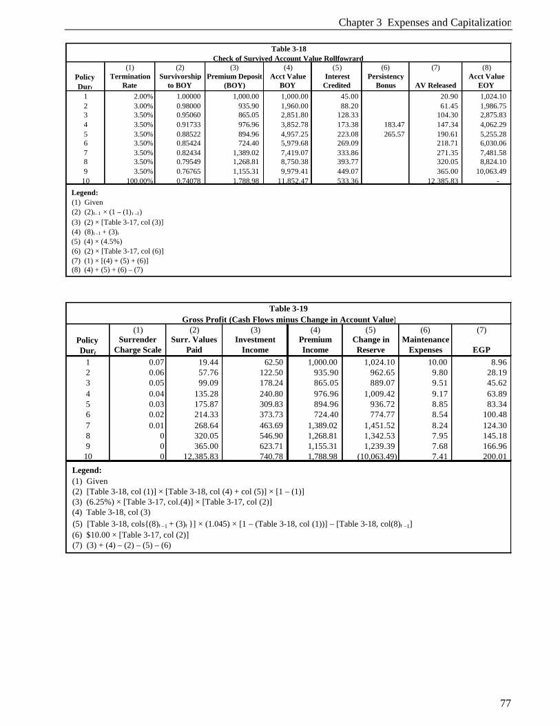
Chapter 3 Expenses and Capitalization

77

(1) (2) (3) (4) (5) (6) (7) (8)Policy Durt

Termination Rate

Survivorship to BOY

Premium Deposit (BOY)

Acct Value BOY

Interest Credited

Persistency Bonus AV Released

Acct Value EOY

1 2.00% 1.00000 1,000.00 1,000.00 45.00 20.90 1,024.10 2 3.00% 0.98000 935.90 1,960.00 88.20 61.45 1,986.75 3 3.50% 0.95060 865.05 2,851.80 128.33 104.30 2,875.83 4 3.50% 0.91733 976.96 3,852.78 173.38 183.47 147.34 4,062.29 5 3.50% 0.88522 894.96 4,957.25 223.08 265.57 190.61 5,255.28 6 3.50% 0.85424 724.40 5,979.68 269.09 218.71 6,030.06 7 3.50% 0.82434 1,389.02 7,419.07 333.86 271.35 7,481.58 8 3.50% 0.79549 1,268.81 8,750.38 393.77 320.05 8,824.10 9 3.50% 0.76765 1,155.31 9,979.41 449.07 365.00 10,063.49

10 100.00% 0.74078 1,788.98 11,852.47 533.36 12,385.83 - Legend: (1) Given (2) (2)t– 1 × (1 – (1) t –1) (3) (2) × [Table 3-17, col (3)] (4) (8)t –1 + (3)t

(5) (4) × (4.5%) (6) (2) × [Table 3-17, col (6)] (7) (1) × [(4) + (5) + (6)] (8) (4) + (5) + (6) – (7)

Check of Survived Account Value RollfowrardTable 3-18

(1) (2) (3) (4) (5) (6) (7)Policy Durt

Surrender Charge Scale

Surr. Values Paid

Investment Income

Premium Income

Change in Reserve

Maintenance Expenses EGP

1 0.07 19.44 62.50 1,000.00 1,024.10 10.00 8.96 2 0.06 57.76 122.50 935.90 962.65 9.80 28.19 3 0.05 99.09 178.24 865.05 889.07 9.51 45.62 4 0.04 135.28 240.80 976.96 1,009.42 9.17 63.89 5 0.03 175.87 309.83 894.96 936.72 8.85 83.34 6 0.02 214.33 373.73 724.40 774.77 8.54 100.48 7 0.01 268.64 463.69 1,389.02 1,451.52 8.24 124.30 8 0 320.05 546.90 1,268.81 1,342.53 7.95 145.18 9 0 365.00 623.71 1,155.31 1,239.39 7.68 166.96 10 0 12,385.83 740.78 1,788.98 (10,063.49) 7.41 200.01

Legend: (1) Given (2) [Table 3-18, col (1)] × [Table 3-18, col (4) + col (5)] × [1 – (1)] (3) (6.25%) × [Table 3-17, col.(4)] × [Table 3-17, col (2)] (4) Table 3-18, col (3) (5) [Table 3-18, cols{(8)t –1 + (3)t }] × (1.045) × [1 – (Table 3-18, col (1))] – [Table 3-18, col(8)t –1] (6) $10.00 × [Table 3-17, col (2)] (7) (3) + (4) – (2) – (5) – (6)

Table 3-19Gross Profit (Cash Flows minus Change in Account Value)

US GAAP for Life Insurers

78

3.12 Worksheet Approaches to DAC Calculation Formulas for benefit reserves, including their maintenance components, and formulas for DAC for specific SFASs are covered in the following chapters. This section presents the features of the worksheet approach to capitalizing and amortizing DAC. The worksheet can be used for a variety of coverages and situations. Chapters 4 (traditional life) and 10 (individual health) address the development of formula-based reserves that are used for factor and first-principles reserve generation. To develop reserves, values are determined per unit and applied to the appropriate units in force on the valuation date. A comparable approach for DAC is known as a worksheet methodology. The worksheet facilitates the exact period deferred acquisition expense to be applied. There is never a question about implied versus actual acquisition expense, as there can be under the formula-based methodology. The worksheet approach operates well with respect to noncommission acquisition expenses. If a worksheet is used for commissions, the level of subsequent heaped renewal commissions must be estimated for each future duration. Depending on the amount of bonuses included in capitalized commissions in the first year, the relationship between the heaped levels and the first-year excess amount deferred can vary and consequently affect the DAC amortization. The worksheet approach can be divided into two types, static and dynamic.

3.12.1 Static Worksheets Table 3-21 illustrates the calculation process for the static worksheet approach. The expense to be deferred is introduced at the beginning of the table. A schedule using mortality and lapse rates is then used to develop an expected in force schedule at future dates. A terminal duration is selected, at which point the DAC will be amortized to zero.

(1) (2) (3) (4) (5) (6) (7) (8) (9) (10)

Policy Durt

Interest Margin

Surrender Charges Expense Charges EGP

Basic DAC Asset

Persistency Bonus PB Liability

Capitalization Pres.Value PB Asset

1 17.50 1.46 10.00 8.96 392.28 29.80 29.80 28.52 25.15 2 34.30 3.69 9.80 28.19 394.77 88.01 56.87 52.08 68.53 3 49.91 5.22 9.51 45.62 388.00 172.43 80.46 70.51 128.41 4 67.42 5.64 9.17 63.89 371.10 183.47 109.89 112.91 94.68 213.96 5 86.75 5.44 8.85 83.34 342.98 265.57 - 150.45 120.73 330.81 6 104.64 4.37 8.54 100.48 304.37 - - - 293.57 7 129.83 2.71 8.24 124.30 251.22 - - - 242.30 8 153.13 - 7.95 145.18 184.44 - - - 177.89 9 174.64 - 7.68 166.96 102.94 - - - 99.29 10 207.42 - 7.41 200.01 (0.00) - - - (0.00)

Present Value of EGP at Crediting Rate: 706.536 Present Value of PB Capitalization: 366.51 DAC Amortization Factor (k1%) 53.78% PB Asset Amortization Rate (k2%) 51.87%

Legend: (1) [Table 3-19, col (3)] – [Table 3-18, col (5)] (2) [Table 3-18, col (1)] × [Table 3-19, col (1)] × [Table 3-18, col (4) + Table 3-18, col(5)] (3) $10.00 × [Table 3-17, col (2)] (4) (1) + (2) – (3) (5) For t = 1, (DAE) × (1.045) – (k1%) × (4)

For t > 1, (5) t = (5)t –1 × (1.045) – (k 1%) × (4) (6) Table 3-18, col(6) (7) Table 3-17, col(10) (8) (7) t – (1.045) × (7)t –1 +(6)t × [Table 3-18, col(1)] × (1 – [Table 3-19, col(1)]) + (6) t × (1 – [Table 3-18, col(1)]) (9) (8) / (1.045

t)

(10) (10)t –1 × (1.045) + (8) t – (k2%) × (4)t

PB Asset Generation

Table 3-20Gross Profits by Source, Bonus Asset & Total DAC Asset

Chapter 8 Variable and Equity-Based Products

277

(1)

(2)

(3)

(4)

(5)

(6)

(7)

(8)

Peri

odPr

emiu

mM

&E

Cha

rges

Surr

ende

r C

harg

es

Def

erra

ble

Acq

uisi

tion

Exp

ense

sM

aint

enan

ce

Per

Polic

yM

orta

lity

Rat

eSu

rren

der

Rat

e

Gro

ss

App

reci

atio

n R

ate

120

,000

1.50

%6.

00%

7.00

%35

0.00

36

1%

-2.0

0%2

-

1.

50%

5.00

%0.

00%

35

0.

0039

2%5.

00%

3-

1.50

%4.

00%

0.00

%35

0.00

43

3%

4.00

%4

-

1.

50%

3.00

%0.

00%

35

0.

0046

4%8.

00%

5-

1.50

%2.

00%

0.00

%35

0.00

50

5%

8.00

%6

-

1.

50%

1.00

%0.

00%

35

0.

0054

6%8.

00%

7-

1.50

%0.

00%

0.00

%35

0.00

58

30

%8.

00%

8-

1.50

%0.

00%

0.00

%35

0.00

64

10

%8.

00%

9-

1.50

%0.

00%

0.00

%35

0.00

70

10

%8.

00%

10-

1.50

%0.

00%

0.00

%35

0.00

76

10

0%8.

00%

Tab

le 8

-25

Var

iabl

e A

nnui

ty G

MD

B P

rovi

sion

Bas

e C

ase

DA

C A

ssum

ptio

ns


278

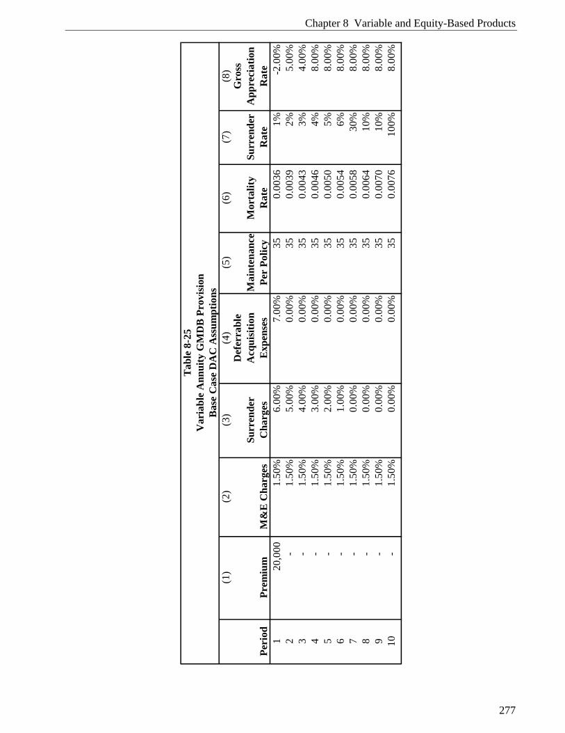
Table 8-26 lists the additional SOP 03-1-related assumptions. Analogous to the DAC assumptions, the first three years’ assumptions are based on historical experience while the remaining years’ assumptions are best estimates as of the end of year 3. Note that the average gross appreciation rate is equal to the gross appreciation rate used for EGPs.

(9) (10)Average Gross

Period Scenario A Scenario B Scenario C Appreciation Rate1 -2.00% -2.00% -2.00% -2.00%2 5.00% 5.00% 5.00% 5.00%3 4.00% 4.00% 4.00% 4.00%4 3.00% 9.00% 12.00% 8.00%5 7.00% -5.00% 22.00% 8.00%6 -12.00% 18.00% 18.00% 8.00%7 9.00% 4.00% 11.00% 8.00%8 15.00% 9.00% 0.00% 8.00%9 2.00% 7.00% 15.00% 8.00%

10 9.00% 2.00% 13.00% 8.00%

Table 8-26Variable Annuity GMDB Provision

Base Case SOP Specific Assumptions

Gross Appreciation Rate


279


280

Table 8-27 shows the policy level development of the scenario-specific account balance and excess death benefit in force, which will be used in the SOP 03-1 liability determination. Similarly, Table 8-28 shows the policy level development of items, which will be used for EGP determination. Note that the account balance in Table 8-28 is based on the deterministic EGP assumptions, but the excess death benefit in force is based on the scenario-specific SOP liability assumptions, which is consistent with the numerical example provided with SOP 03-1.

(1)

(2)

(3)

(4)

(5)

Acc

ount

Bal

ance

Prem

ium

+Pe

riod

Scen

ario

ASc

enar

io B

Scen

ario

C5%

Inte

rest

Scen

ario

ASc

enar

io B

Scen

ario

CSc

enar

io A

Scen

ario

BSc

enar

io C

Ave

rage

119

,300

.00

19,3

00.0

0

19

,300

.00

21

,000

.00

21

,000

.00

21,0

00.0

0

21,0

00.0

0

1,70

0.00

1,

700.

00

1,

700.

00

1,

700.

00

219

,975

.50

19,9

75.5

0

19

,975

.50

22

,050

.00

22

,050

.00

22,0

50.0

0

22,0

50.0

0

2,07

4.50

2,

074.

50

2,

074.

50

2,

074.

50

320

,474

.89

20,4

74.8

9

20

,474

.89

23

,152

.50

23

,152

.50

23,1

52.5

0

23,1

52.5

0

2,67

7.61

2,

677.

61

2,

677.

61

2,

677.

61

420

,782

.01

22,0

10.5

0

22

,624

.75

24

,310

.13

24

,310

.13

24,3

10.1

3

24,3

10.1

3

3,52

8.11

2,

299.

62

1,

685.

37

2,

504.

37

521

,925

.02

20,5

79.8

2

27

,262

.82

25

,525

.63

25

,525

.63

25,5

25.6

3

27,2

62.8

2

3,60

0.61

4,

945.

81

-

2,

848.

81

618

,965

.14

23,9

75.4

9

31

,761

.19

26

,801

.91

26

,801

.91

26,8

01.9

1

31,7

61.1

9

7,83

6.77

2,

826.

42

-

3,

554.

40

720

,387

.53

24,5

74.8

8

34

,778

.50

28

,142

.01

28

,142

.01

28,1

42.0

1

34,7

78.5

0

7,75

4.48

3,

567.

13

-

3,

773.

87

823

,139

.85

26,4

18.0

0

34

,256

.83

29

,549

.11

29

,549

.11

29,5

49.1

1

34,2

56.8

3

6,40

9.26

3,

131.

11

-

3,

180.

13

923

,255

.54

27,8

70.9

8

38

,881

.50

31

,026

.56

31

,026

.56

31,0

26.5

6

38,8

81.5

0

7,77

1.02

3,

155.

58

-

3,

642.

20

1024

,999

.71

28,0

10.3

4

43

,352

.87

32

,577

.89

32

,577

.89

32,5

77.8

9

43,3

52.8

7

7,57

8.18

4,

567.

55

-

4,

048.

58

Leg

end:

(1)

A

ccou

nt B

alan

ce (1

) t =

((1)

t–1

+ Ta

ble

8-25

col

umn

(1) t

) × (1

+ T

able

8-2

6 co

lum

n (9

) t –

Tabl

e 8-

25 c

olum

n (2

) t).

(2)

Pr

emiu

m +

5%

Inte

rest

(2) t

= ((

2)t–

1 + T

able

8-2

5 co

lum

n (1

) t) ×

1.0

5.(3

)

Dea

th B

enef

it A

ccou

nt B

alan

ce =

max

imum

((1)

t, (2

) t).

(4)

Ex

cess

Dea

th B

enef

it In

forc

e (4

) t =

(3) t

– (1

) t.

(5)

A

vera

ge D

eath

Ben

efit

Info

rce

(5) t

= A

vera

ge o

f (4)

t Sce

nario

s A, B

, C.

Var

iabl

e A

nnui

ty G

MD

B P

rovi

sion

Bas

e C

ase

Polic

y L

evel

Exp

erie

nce

for

SOP

03-1

Add

ition

al L

iabi

lity

Cal

cula

tion

Dea

th B

enef

it A

ccou

nt B

alan

ceE

xces

s Dea

th B

enef

it In

forc

e

Tab

le 8

-27


281


286

8.2.5.6 GMAB Tables 8-34 through 8-38 provide a base case example of a single premium variable deferred annuity with a GMAB provision. This example illustrates a method of calibrating the required profit margin at issue and how a liability valuation formula is derived. The GMAB rider benefit is a return of premium at the end of 10 years and the rider charges are specified. Table 8-34 lists the best estimate non-economic assumptions, and Table 8-35 lists the economic assumptions, all as of the issue date. In this example, the average of the scenario-specific gross appreciation rate assumptions equals the risk-free forward interest rates, implying that the assumptions are market consistent. (In practice, the volatility of returns should also calibrate to the implied volatility observed in the market.)

(1) (2) (3) (4) (5)M&E Charges for Charges for Mortality Surrender

Period Premium Base Policy GMAB Rate Rate1 20,000 1.50% 1.00% 0.0036 1%2 - 1.50% 1.00% 0.0039 2%3 - 1.50% 1.00% 0.0043 3%4 - 1.50% 1.00% 0.0046 4%5 - 1.50% 1.00% 0.0050 5%6 - 1.50% 1.00% 0.0054 6%7 - 1.50% 1.00% 0.0058 30%8 - 1.50% 1.00% 0.0064 10%9 - 1.50% 1.00% 0.0070 10%10 - 1.50% 1.00% 0.0076 100%

Table 8-34Variable Annuity GMAB Provision

Base Case Best Estimate Assumptions

(6) (7) (8)Forward Rate Curve Average Gross Risk-free

Period Scenario A Scenario B Scenario C Appreciation Rate Forward Rate1 2.25% -4.75% 9.25% 2.25% 2.25%2 -1.00% -3.50% 12.00% 2.50% 2.50%3 1.50% 3.50% 2.50% 2.50% 2.50%4 -2.00% 4.00% 7.00% 3.00% 3.00%5 1.25% -9.25% 17.75% 3.25% 3.25%6 -16.50% 13.50% 13.50% 3.50% 3.50%7 4.75% -0.25% 6.75% 3.75% 3.75%8 11.00% 5.00% -4.00% 4.00% 4.00%9 -1.75% 3.25% 11.25% 4.25% 4.25%

10 3.50% -1.50% 11.50% 4.50% 4.50%

Table 8-35Variable Annuity GMAB Provision

Base Case GMAB Economic Assumptions

Gross Appreciation Rate


296

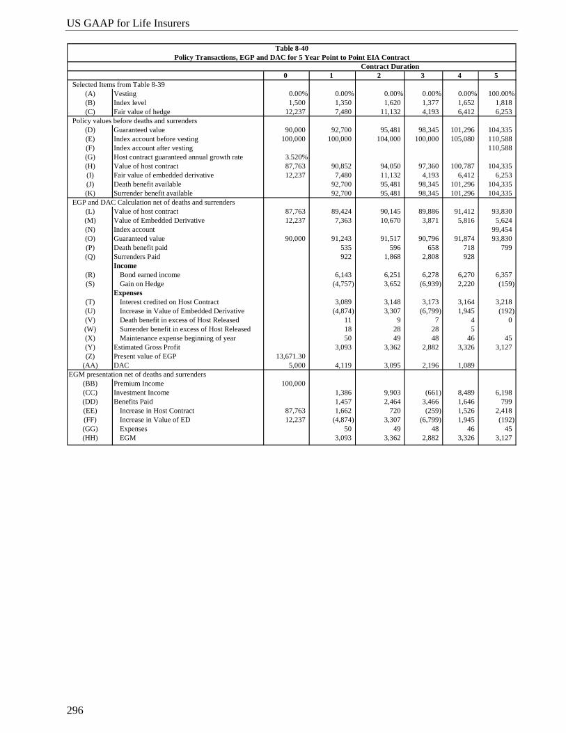
0 1 2 3 4 5 Selected Items from Table 8-39

(A) Vesting 0.00% 0.00% 0.00% 0.00% 0.00% 100.00%(B) Index level 1,500 1,350 1,620 1,377 1,652 1,818 (C) Fair value of hedge 12,237 7,480 11,132 4,193 6,412 6,253

Policy values before deaths and surrenders(D) Guaranteed value 90,000 92,700 95,481 98,345 101,296 104,335 (E) Index account before vesting 100,000 100,000 104,000 100,000 105,080 110,588 (F) Index account after vesting 110,588 (G) Host contract guaranteed annual growth rate 3.520%(H) Value of host contract 87,763 90,852 94,050 97,360 100,787 104,335 (I) Fair value of embedded derivative 12,237 7,480 11,132 4,193 6,412 6,253 (J) Death benefit available 92,700 95,481 98,345 101,296 104,335 (K) Surrender benefit available 92,700 95,481 98,345 101,296 104,335

EGP and DAC Calculation net of deaths and surrenders(L) Value of host contract 87,763 89,424 90,145 89,886 91,412 93,830 (M) Value of Embedded Derivative 12,237 7,363 10,670 3,871 5,816 5,624 (N) Index account 99,454 (O) Guaranteed value 90,000 91,243 91,517 90,796 91,874 93,830 (P) Death benefit paid 535 596 658 718 799 (Q) Surrenders Paid 922 1,868 2,808 928

Income(R) Bond earned income 6,143 6,251 6,278 6,270 6,357 (S) Gain on Hedge (4,757) 3,652 (6,939) 2,220 (159)

Expenses(T) Interest credited on Host Contract 3,089 3,148 3,173 3,164 3,218 (U) Increase in Value of Embedded Derivative (4,874) 3,307 (6,799) 1,945 (192) (V) Death benefit in excess of Host Released 11 9 7 4 0 (W) Surrender benefit in excess of Host Released 18 28 28 5 (X) Maintenance expense beginning of year 50 49 48 46 45 (Y) Estimated Gross Profit 3,093 3,362 2,882 3,326 3,127 (Z) Present value of EGP 13,671.30

(AA) DAC 5,000 4,119 3,095 2,196 1,089 EGM presentation net of deaths and surrenders

(BB) Premium Income 100,000 (CC) Investment Income 1,386 9,903 (661) 8,489 6,198 (DD) Benefits Paid 1,457 2,464 3,466 1,646 799 (EE) Increase in Host Contract 87,763 1,662 720 (259) 1,526 2,418 (FF) Increase in Value of ED 12,237 (4,874) 3,307 (6,799) 1,945 (192) (GG) Expenses 50 49 48 46 45 (HH) EGM 3,093 3,362 2,882 3,326 3,127

Contract Duration

Table 8-40Policy Transactions, EGP and DAC for 5 Year Point to Point EIA Contract


297

Table 8-41 displays the resulting balance sheet and income statements for the product. For the sake of clarity, the bonds are assumed to be classified as held to maturity and are therefore reported at amortized cost. Their value has been diminished by cash needed to pay maintenance expenses, death claims, and surrenders. Earnings are volatile because they are affected by the changing value of the index each year. The major contributing factor to this volatility is the unequal amounts in the early years of hedge and embedded options.

Legend:(A) From Table 8-39, (H).(B) From Table 8-39, (N).(C) From Table 8-39, (Z).(D) (D)t = (D)t –1 × [1 + (C)0 from Table 8-39]; initial value (D)0 = (A)0 × [1 – (B)0]; (A), (B) and (C) are from Table 8-39.(E) (E)t = Max [(A)0, (A)0 × {1 + (F)0 × [(N)t / (N)0 – 1]}]; initial value (F)0 = (A)0; (A), (F) and (N) are from Table 8-39.(F) = (E)t × (A)t.

(G) = {[(R)0 / (H)0] ^ (1/5)} – 1; (R)0 is from Table 8-39.(H) (H)0 = (A)0 – (Y)0; (H)t = (H)t –1 × [1 + (G)0] for t = 1 to 5. (A) and (Y) are from Table 8-39.(I) From Table 8-39, (Y).(J) = (D)t.

(K) = (D)t.

(L) = (H)t × (L)t ; (L) is from Table 8-39.(M) = (I)t × (L)t ; (L) is from Table 8-39.(N) = (F)t × (L)t ; (L) is from Table 8-39.(O) = (D)t – (L)t ; (L) is from Table 8-39.(P) = (J)t × (L)t –1 × (J)t / 1000; (L) and second (J) are from Table 8-39.(Q) = [(K)t × (L)t –1 × (1 – Jt / 1000)] × (K)t ; (L) and second (K) are from Table 8-39.(R) = [(L)t –1 + (M)t –1 – (C)t –1] × (G)0 where (G) is from Table 8-39.(S) = (C)t – (C)t –1.

(T) = (L)t –1 × (G)0.

(U) = (M)t – (M)t –1.

(V) = [(J)t – (H)t ] × (L)t –1 × (J)t / 1000; (L) and second (J) are from Table 8-39.(W) = [(K)t – (H)t ] × (L)t –1 × (J)t / 1000 × (K)t ; (L), (J) and second (K) are from Table 8-39.(X) = (D)0 × (L)t –1 from Table 8-39.(Y) = (R)t + (S)t – (T)t – (U)t – (V)t – (W)t – (X)t.

(Z) Present value of the EGP (Y) at issue date discounted at earned rate (G)t less 200 basis points, where (G) is from Table 8-39.(AA) = (AA)t –1 × [1 + (G)0 – 0.02] – (Y)t × (AA)0 / (Z)0; (AA)0 = (A)0 × (E)0 where (A), (E) and (G) are from Table 8-39.(BB) = Table 8-39 (A)t.

(CC) = (R)t + (S)t.

(DD) = (P)t + (Q)t.

(EE) = (L)t – (L)t –1.

(FF) = (M)t – (M)t –1; (FF)0 = I0.

(GG) = (X)t.

(HH) = (BB)t + (CC)t – (DD)t – (EE)t – (FF)t – (GG)t.

Table 8-40 ContinuedPolicy Transactions, EGP and DAC for 5 Year Point to Point EIA Contract


298

0 1 2 3 4 5 Items from Table 8-39

(A) Deposit 100,000 (B) Zero-coupon bond rate 7.00%

Items from Table 8-40(C) Index account 99,454 (D) Guaranteed value 90,000 91,243 91,517 90,796 91,874 93,830 (E) Premium Income 100,000 (F) Investment Income for EGP 1,386 9,903 (661) 8,489 6,198 (G) DAC 5,000 4,119 3,095 2,196 1,089 (H) Estimated Gross Profit 3,093 3,362 2,882 3,326 3,127

Balance SheetAssets

(I) Bonds held to maturity 82,763 87,046 90,623 93,449 98,295 104,327 (J) Fair value of hedge 12,237 7,480 11,132 4,193 6,412 6,253 (K) DAC 5,000 4,119 3,095 2,196 1,089 (L) Total assets 100,000 98,645 104,850 99,838 105,796 110,581

Liabilities(M) Value of host contract 87,763 89,424 90,145 89,886 91,412 93,830 (N) Value of embedded derivative 12,237 7,363 10,670 3,871 5,816 5,624 (O) Total liabilities 100,000 96,787 100,815 93,757 97,228 99,454 (P) Equity 1,858 4,035 6,080 8,568 11,126 (Q) Change in equity 1,858 2,177 2,045 2,488 2,558

Income StatementRevenues

(R) Investment income on bonds 0 5,790 6,090 6,340 6,538 6,877(S) Gain on Hedge (4,757) 3,652 (6,939) 2,220 (159) (T) Total revenues 0 1,033 9,742 (599) 8,758 6,718

Expenses(U) Interest credited on host contract 0 3,089 3,148 3,173 3,164 3,218(V) Death benefit in excess of Host Released 11 9 7 4 0(W) Surrender benefit in excess of Host Released 18 28 28 5 0(X) Maintenance cost 0 50 49 48 46 45(Y) Acquisition cost expense 0 881 1,024 899 1,107 1,089(Z) Increase in Value of Embedded Derivative (4,874) 3,307 (6,799) 1,945 (192)

(AA) Total expenses 0 (825) 7,565 (2,644) 6,270 4,160(BB) Net income 0 1,858 2,177 2,045 2,488 2,558

Contract Duration

Table 8-41Balance Sheet and Income Statement for 5 Yr Point to Point EIA Contract


299

8.3.4.2 Annual Ratchet EIA Product The following tables will illustrate how SFAS 133 accounting can be applied to an annual

ratchet product. They start with many of the same basic experience assumptions used in the point-to-point example in Section 8.3.4.1 and show results through the first five calendar years after issue. Tables 8-42, 8-43, and 8-44 are determined at the beginning of year 1 (t = 0). Tables 8-45, 8-46, and 8-47 are determined at the beginning of year 2 (t = 1) and reflect the impact of the first-year option benefits expiring in the money. Only a single deposit at issue is assumed for all of the tables.

Table 8-42 illustrates basic features of the ratchet EIA contract. The Capital Markets section shows the expected budgeted amounts (the amounts available to provide call options to the policyholders based upon pricing). Budgeted amounts are assumed to be fully available at the beginning of each year. Assumptions used for Black-Scholes calculations are also presented. At issue, the assumed participation rate of 41.15% has been scaled so that the initial option equals the budget. The strike price for the option is equal to the initial index value. The at-the-money nature of the option reflects the fact that projected guaranteed benefits at the end of year 1 don’t exceed the index value from the beginning of the year.

Legend(A) From Table 8-39, (A).(B) From Table 8-39, (G).(C) From Table 8-40, (N).(D) From Table 8-40, (O).(E) From Table 8-40, (BB).(F) From Table 8-40, (CC) (G) From Table 8-40, (HH).(H) From Table 8-40, (Y).(I) (I)t = [(I)t– 1 – (X)t ] × [1 + (G)0] – (P)t – (Q)t ; initial value (I)0 = (A)0 × [1 – (E)0] – (Z)0

where (A), (E), (G) and (Z) come from Table 8-39; (X), (P) and (Q) from Table 8-40.(J) = (C)t from Table 8-40.(K) = (G)t from Table 8-41.(L) = (I)t + (J)t + (K)t.

(M) = (L)t from Table 8-40.(N) = (M)t from Table 8-40.(O) = (M)t + (N)t.

(P) = (L)t – (O)t.

(Q) = (P)t – (P)t– 1.

(R) = [(I)t– 1 – (X)t ] × (B)0 where (X) is from Table 8-40. (S) = (S)t from Table 8-40.(T) = (R)t + (S)t.

(U) = (T)t from Table 8-40. (V) = (V)t from Table 8-40.(W) = (W)t from Table 8-40.(X) = (X)t from Table 8-40. (Y) = (AA)t– 1 – (AA)t from Table 8-40.(Z) = (U)t from Table 8-40.

(AA) = (U)t + (V)t + (W)t + (X)t + (Y)t + (Z)t.

(BB) = (T)t – (AA)t.

Table 8-41 ContinuedBalance Sheet and Income Statement for 5 Yr Point to Point EIA Contract


300

0 1 2 3 4 5 Contract Design and Pricing Assumptions

(A) Deposit $100,000(B) Policy load 10.00%(C) Guaranteed interest rate 3.00%(D) Maintenance expense $50.00(E) Acquisition cost as percentage of premium 5%(F) Participation rate 41.15%(G) Zero-coupon bond rate 7.00% 7.00% 7.00% 7.00% 7.00% 7.00%(H) Mortality rate per 1,000 5.77 6.35 6.98 7.68 8.45(I) Lapse rate 1.00% 2.00% 3.00% 1.00% 0.00%(J) Surrender charge 10.00% 10.00% 10.00% 10.00% 10.00%(K) Contracts persisting (prior to maturity) 1.00000 0.98429 0.95848 0.92323 0.90698 0.89932(L) Maturity rate 0.00% 0.00% 0.00% 0.00% 100.00%

Capital Markets(M) Option budget 4.50% 4.50% 4.50% 4.50% 4.50%(N) Index level 1,500 (O) Implied volatility 22.0%(P) Risk-free rate 6.00% 6.00% 6.00% 6.00% 6.00% 6.00%(Q) Dividend rate 1.25%

Calculation of Account, Guaranteed, and Option Values(R) Index account 100,000 104,770 109,768 115,003 120,489 126,236(S) Guaranteed value 90,000 92,700 95,481 98,345 101,296 104,335

BOY(T) Strike price for annual hedge 1,500 (U) Time to expiry for annual hedge 1.0000000(V) D1 0.33(W) D2 0.11(X) Black-Scholes price 164.03(Y) Fair value of hedge 4,500 4,715 4,940 5,175 5,422

EOY(Z) Fair value of hedge 4,770 4,998 5,236 5,486 5,747

Legend:(A) to (F) Policy features and assumptions.(G) to (I) Experience assumptions.

(J) Annual Surrender Charge.(K) (K)0 = 1; For t > 0, (K)t = (K)t –1 × [1 – (H)t / 1000] × [1 – (I)t ].

(L) to (Q) Assumptions(R) (R)0 = (A)0; For t = 1–5, (R)t = (R)t –1 + (Z)t .(S) (S)t = [1 – (B)0] × (A)0 × [1 + (C)0] ^ t.

Beginning of Year Hedge Values(T) (T)t = (O)t –1

(U) One-year hedge purchased at the beginning of the year.(V) Black-Scholes Parameter D1 = (V)t = [ln [(N)t –1 / (T)t ] + [(P)t –1 – (Q)t –1 + (O)t –1 ^ 2 / 2] × (U)t ] / [(O)t –1 × (U)t ^ 0.5].(W) Black-Scholes Parameter D2 = (W)t = (Vt ) – (O)t –1 × (U)t ^ 0.5.(X) (X)t = (N)t –1 × EXP[–(Q)t –1 × (U)t ] × NORMDIST[(V)t ] – (T)t × EXP[–(P)t –1 × (U)t ] × NORMDIST[(W)t ].(Y) For t = 1, (Y)t = (R)t –1 × (F)0 × (X)t / (N)t –1; For t = 2–5, (Y)t = (R)t –1 × (M)t .

Year Hedge Values(Z) (Z)t = (R)t –1 × (M)t × [1 + (P)t ].

Table 8-42Annual Ratchet EIA Product Design and Pricing Assumptions (Valuation Date t = 0)

Contract Duration


302

Legend:(A) From Table 8-42, (S)t .(B) From Table 8-42, (R)t .(C) From Table 8-42, For t = 0, (Y)1; For t > 0, (Z)t .(D) (D)t = (B)t – (B)t –1 – (A)t ; (A)t is from Table 8-42.(E) (E)t = (B)t .(F) (F)t = (B)t .(G) (G)t = (B)t × (K)t ; (K)t is from Table 8-42.(H) (H)t = (A)t × (K)t ; (K)t is from Table 8-42.(I) (I)t = (E)t –1 × (K)t –1 × (H)t / 1000; (K)t and (H)t are from Table 8-42.(J) (J)t = (F)t –1 × (K)t –1 × [1 – (H)t / 1000] × (I)t ; (K)t , (H)t and (I)t are from Table 8-42.(K) (K)t = (G)t × (L)t ; (L)t is from Table 8-42.(L) (L)t = [(I)t + (J)t + (K)t ] × (H)t –1 / (G)t –1.(M) (M)t = [(I)t + (J)t + (K)t ] – (L)t .(N) (N)5 = 0; For t = 4 to 0, (N)t = [(N)t +1 + (M)t +1] / [1 + (P)t ]; (P)t is from Table 8-42.(O) Internal rate of return based on Host Cash Flow (P)0 through (P)5.(P) For t = 0, (P)0 = (A)0 – (N)0 – (L)0; (A)0 is from Table 8-42; For t > 0, (P)t = –(L)t .(Q) For t = 0, (Q)0 = (P)0; For t > 0, (Q)t = (Q)t –1 × [1 + (O)0] + (P)t .(R) (R)t = [(N)t –1 + (Q)t –1 – (C)t –1 × (K)t –1] × (G)0; (G)0 and (K)t –1 are from Table 8-42.(S) (S)t = [(Z)t – (Y)t ] × (K)t –1; (Z)t , (Y)t and (K)t –1 are from Table 8-42.(T) (T)t = (J)t × (J)t ; (J)t is from Table 8-42.(U) (U)t = (Q)t × (O)0.(V) (V)t = (N)t – (N)t –1 + (M)t .(W) (W)t = (D)0 × (K)t –1; (D)0 × (K)t –1 are from Table 8-42.(X) (X)t = (R)t + (S)t + (T)t – (U)t – (V)t – (W)t .(Y) Present value of the EGP (X)t at issue date discounted at earned rate (G)t less 250 basis points; (G)t is from Table 8-42.(Z) (Z)t = (A)t × (E)t ; (A)t and (E)t are from Table 8-42.

(AA) (AA)0 = (Z)0 / (Y)0.(BB) (BB)0 = (Z)0; For t > 0, (BB)t = (BB)t –1 × [1 + (G)t – 0.025] + (Z)t – (AA)0 × (X)t ; (G)t is from Table 8-42.(CC) (CC)t = (A)t ; (A)t is from Table 8-42.(DD) (DD)t = (R)t + (S)t .(EE) (EE)t = (I)t + (J)t + (K)t – (T)t .(FF) (FF)t = (Q)t – (Q)t –1.(GG) (GG)t = (N)t – (N)t –1.(HH) (HH)t = (W)t .(II) (II)t = (CC)t + (DD)t – (EE)t – (FF)t – (GG)t – (HH)t .

Policy Transactions, EGP and DAC for Annual Ratchet EIA Contract (Valuation Date t = 0)Table 8-43 Continued


303

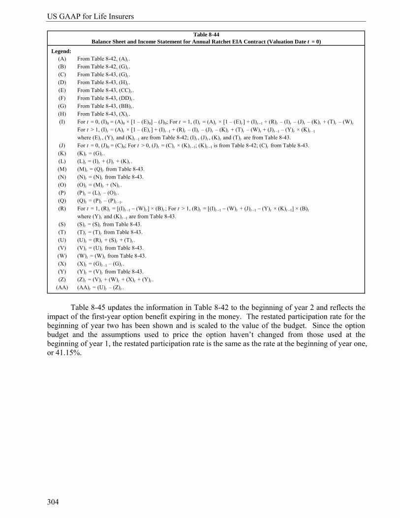
Table 8-44 displays the resulting balance sheet and income statements.


(A) Deposit 100,000 (B) Zero-coupon bond rate 7.00% 7.00% 7.00% 7.00% 7.00% 7.00%

Items from Table 8-43(C) Index account 100,000 103,124 105,210 106,175 109,281 113,527(D) Guaranteed value 90,000 91,243 91,517 90,796 91,874 93,830(E) Premium Income 100,000(F) Investment Income 6,955 7,166 7,312 7,385 7,600(G) DAC 5,000 4,152 3,188 2,110 1,070 0(H) Estimated Gross Profit 0 2,343 2,512 2,666 2,478 2,441

Balance SheetAssets

(I) Bonds held to maturity 90,500 95,310 99,568 103,129 108,792 2,066(J) Fair value of hedge 4,500 4,770 4,919 5,019 5,065 5,213(K) DAC 5,000 4,152 3,188 2,110 1,070 0(L) Total assets 100,000 104,231 107,675 110,257 114,927 7,279

Liabilities(M) Value of host contract 85,314 87,680 89,172 89,758 92,137 0(N) Fair value of embedded derivative 14,686 15,410 16,023 16,481 17,199 0(O) Total liabilities 100,000 103,090 105,196 106,239 109,336 0(P) Equity 0 1,141 2,479 4,018 5,591 7,279(Q) Change in equity 1,141 1,338 1,539 1,572 1,688


(R) Investment income on bonds 6,331 6,677 6,979 7,233 7,623(S) Gain on Hedge 270 278 284 287 295(T) Surrender Charge 99 205 313 105 0(U) Total revenues 6,701 7,161 7,577 7,625 7,918

Expenses(V) Interest credited on host contract 3,780 3,885 3,951 3,977 4,082(W) Maintenance cost 50 49 48 46 45(X) Acquisition cost expense 848 964 1,078 1,040 1,070(Y) Increase in Value of Embedded Derivative 881 925 961 989 1,032(Z) Total expenses 5,560 5,823 6,038 6,052 6,229

(AA) Net income 1,141 1,338 1,539 1,572 1,688

Table 8-44Balance Sheet and Income Statement for Annual Ratchet EIA Contract (Valuation Date t = 0)

Contract Duration


304

Table 8-45 updates the information in Table 8-42 to the beginning of year 2 and reflects the

impact of the first-year option benefit expiring in the money. The restated participation rate for the beginning of year two has been shown and is scaled to the value of the budget. Since the option budget and the assumptions used to price the option haven’t changed from those used at the beginning of year 1, the restated participation rate is the same as the rate at the beginning of year one, or 41.15%.

Legend:(A) From Table 8-42, (A)t .(B) From Table 8-42, (G)t .(C) From Table 8-43, (G)t .(D) From Table 8-43, (H)t .(E) From Table 8-43, (CC)t .(F) From Table 8-43, (DD)t .(G) From Table 8-43, (BB)t .(H) From Table 8-43, (X)t .(I) For t = 0, (I)0 = (A)0 × [1 – (E)0] – (J)0; For t = 1, (I)t = (A)t × [1 – (E)t ] + (I)t –1 + (R)t – (I)t – (J)t – (K)t + (T)t – (W)t

For t > 1, (I)t = (A)t × [1 – (E)t ] + (I)t –1 + (R)t – (I)t – (J)t – (K)t + (T)t – (W)t + (J)t –1 – (Y)t × (K)t –1

where (E)t , (Y)t and (K)t –1 are from Table 8-42; (I)t , (J)t , (K)t and (T)t are from Table 8-43.(J) For t = 0, (J)0 = (C)0; For t > 0, (J)t = (C)t × (K)t –1; (K)t –1 is from Table 8-42; (C)t from Table 8-43.(K) (K)t = (G)t .(L) (L)t = (I)t + (J)t + (K)t .(M) (M)t = (Q)t from Table 8-43.(N) (N)t = (N)t from Table 8-43.(O) (O)t = (M)t + (N)t .(P) (P)t = (L)t – (O)t .(Q) (Q)t = (P)t – (P)t –1.(R) For t = 1, (R)t = [(I)t –1 – (W)t ] × (B)t ; For t > 1, (R)t = [(I)t –1 – (W)t + (J)t –1 – (Y)t × (K)t –1] × (B)t

where (Y)t and (K)t –1 are from Table 8-43.(S) (S)t = (S)t from Table 8-43.(T) (T)t = (T)t from Table 8-43.(U) (U)t = (R)t + (S)t + (T)t .(V) (V)t = (U)t from Table 8-43.(W) (W)t = (W)t from Table 8-43.(X) (X)t = (G)t –1 – (G)t .(Y) (Y)t = (V)t from Table 8-43.(Z) (Z)t = (V)t + (W)t + (X)t + (Y)t .

(AA) (AA)t = (U)t – (Z)t .

Balance Sheet and Income Statement for Annual Ratchet EIA Contract (Valuation Date t = 0)Table 8-44


307

Table 8-47 shows the restated balance sheets and income statements. The balance sheet at t = 1 and the income statement for year 1 are actual. The items for the remaining periods are projected.

Legend:(A) From Table 8-45, (T)t .(B) From Table 8-45, (S)t .(C) From Table 8-45, For t = 0, (Z)1; For t > 0, (FF)t .(D) (D)t = (B)t – (B)t –1 – (A)t ; (A)t is from Table 8-45.(E) (E)t = (B)t .(F) (F)t = (B)t .(G) (G)t = (B)t × (K)t ; (K)t is from Table 8-45.(H) (H)t = (A)t × (K)t ; (K)t is from Table 8-45.(I) (I)t = (E)t –1 × (K)t –1 × (H)t / 1000; (K)t and (H)t are from Table 8-45.(J) (J)t = (F)t –1 × (K)t –1 × [1 – (H)t / 1000] × (I)t ; (K)t , (H)t and (I)t are from Table 8-45.(K) (K)t = (G)t × (L)t ; (L)t is from Table 8-45.(L) (L)t = [(I)t + (J)t + (K)t ] × (H)t –1 / (G)t –1.(M) (M)t = [(I)t + (J)t + (K)t ] – (L)t .(N) (N)5 = 0; For t = 4 to 1, (N)t = [(N)t +1 + (M)t +1] / [1 + (Q)t ]; (Q)t is from Table 8-45

(N)0 = (N)0 from Table 8-43.(O) Internal rate of return based on Host Cash Flow (P)0 through (P)5.(P) For t = 0, (P)0 = (A)0 – (N)0 – (L)0; (A)0 is from Table 8-45; For t > 0, (P)t = –(L)t .(Q) For t = 0, (Q)0 = (P)0; For t > 0, (Q)t = (Q)t –1 × [1 + (O)0] + (P)t .(R) (R)t = [(N)t –1 + (Q)t –1 – (C)t –1 × (K)t –1] × (G)0; (G)0 and (K)t –1 are from Table 8-45.(S) (S)t = [(FF)t – (Z)t ] × (K)t –1; (FF)t , (Z)t and (K)t –1 are from Table 8-45.(T) (T)t = (J)t × (J)t ; (J)t is from Table 8-45.(U) (U)t = (Q)t × (O)0.(V) (V)t = (N)t – (N)t –1 + (M)t .(W) (W)t = (D)0 × (K)t –1; (D)0 × (K)t –1 are from Table 8-45.(X) (X)t = (R)t + (S)t + (T)t – (U)t – (V)t – (W)t .(Y) Present value of the EGP (X)t at issue date discounted at earned rate (G)t less 250 basis points; (G)t is from Table 8-45.(Z) (Z)t = (A)t × (E)t ; (A)t and (E)t are from Table 8-45.

(AA) (AA)0 = (Z)0 / (Y)0.(BB) (BB)0 = (Z)0; For t > 0, (BB)t = (BB)t –1 × [1 + (G)t – 0.025] + (Z)t – (AA)0 × (X)t ; (G)t is from Table 8-45.(CC) (CC)t = (A)t ; (A)t is from Table 8-45.(DD) (DD)t = (R)t + (S)t .(EE) (EE)t = (I)t + (J)t + (K)t – (T)t .(FF) (FF)t = (Q)t – (Q)t –1.(GG) (GG)t = (N)t – (N)t –1.(HH) (HH)t = (W)t .(II) (II)t = (CC)t + (DD)t – (EE)t – (FF)t – (GG)t – (HH)t .

Policy Transactions, EGP and DAC for Annual Ratchet EIA Contract (Valuation Date t = 1)Table 8-46 Continued


308


(A) Deposit 100,000 (B) Zero-coupon bond rate 7.00% 7.00% 7.00% 7.00% 7.00% 7.00%

Items from Table 8-46(C) Index account 100,000 102,479 104,552 105,511 108,598 112,817(D) Guaranteed value 90,000 91,243 91,517 90,796 91,874 93,830(E) Premium Income 100,000(F) Investment Income 6,300 7,166 7,268 7,340 7,553(G) DAC 5,000 4,168 3,186 2,109 1,069 0(H) Estimated Gross Profit 0 2,302 2,548 2,658 2,472 2,434

Balance SheetAssets

(I) Bonds held to maturity 90,500 95,310 98,914 102,450 108,075 2,013(J) Fair value of hedge 4,500 4,115 4,888 4,987 5,033 5,180(K) DAC 5,000 4,168 3,186 2,109 1,069 0(L) Total assets 100,000 103,593 106,988 109,546 114,177 7,194

Liabilities(M) Value of host contract 85,314 87,680 89,172 89,758 92,137 0(N) Fair value of embedded derivative 14,686 14,796 15,389 15,833 16,524 0(O) Total liabilities 100,000 102,476 104,562 105,591 108,661 0(P) Equity 0 1,117 2,427 3,955 5,517 7,194(Q) Change in equity 1,117 1,310 1,528 1,562 1,677


(R) Investment income on bonds 6,331 6,633 6,933 7,185 7,572(S) Gain on Hedge (385) 277 282 285 293(T) Surrender Charge 99 204 311 105 0(U) Total revenues 6,046 7,114 7,527 7,575 7,866

Expenses(V) Interest credited on host contract 3,780 3,885 3,951 3,977 4,082(W) Maintenance cost 50 49 48 46 45(X) Acquisition cost expense 832 982 1,077 1,040 1,069(Y) Increase in Value of Embedded Derivative 267 888 923 950 991(Z) Total expenses 4,929 5,804 5,999 6,013 6,189

(AA) Net income 1,117 1,310 1,528 1,562 1,677

Table 8-47Balance Sheet and Income Statement for Annual Ratchet EIA Contract (Valuation Date t = 1)

Contract Duration


309

Legend:(A) From Table 8-45, (A)t .(B) From Table 8-45, (G)t .(C) From Table 8-46, (G)t .(D) From Table 8-46, (H)t .(E) From Table 8-46, (CC)t .(F) From Table 8-46, (DD)t .(G) From Table 8-46, (BB)t .(H) From Table 8-46, (X)t .(I) For t = 0, (I)0 = (A)0 × [1 – (E)0] – (J)0; For t = 1, (I)t = (A)t × [1 – (E)t ] + (I)t –1 + (R)t – (I)t – (J)t – (K)t + (T)t – (W)t

For t > 1, (I)t = (A)t × [1 – (E)t ] + (I)t –1 + (R)t – (I)t – (J)t – (K)t + (T)t – (W)t + (J)t –1 – (Z)t × (K)t –1

where (E)t , (Z)t and (K)t– 1 are from Table 8-45; (I)t , (J)t , (K)t and (T)t are from Table 8-46.(J) For t = 0, (J)0 = (C)0; For t > 0, (J)t = (C)t × (K)t –1; (K)t –1 is from Table 8-45; (C)t from Table 8-46.(K) (K)t = (G)t .(L) (L)t = (I)t + (J)t + (K)t .(M) (M)t = (Q)t from Table 8-46.(N) (N)t = (N)t from Table 8-46.(O) (O)t = (M)t + (N)t .(P) (P)t = (L)t – (O)t .(Q) (Q)t = (P)t – (P)t –1.(R) For t = 1, (R)t = [(I)t –1 – (W)t ] × (B)t ; For t > 1, (R)t = [(I)t –1 – (W)t + (J)t –1 – (Z)t × (K)t –1] × (B)t

where (Z)t and (K)t –1 are from Table 8-46.(S) (S)t = (S)t from Table 8-46.(T) (T)t = (T)t from Table 8-46.(U) (U)t = (R)t + (S)t + (T)t .(V) (V)t = (U)t from Table 8-46.(W) (W)t = (W)t from Table 8-46.(X) (X)t = (G)t –1 – (G)t .(Y) (Y)t = (V)t from Table 8-46.(Z) (Z)t = (V)t + (W)t + (X)t + (Y)t .

(AA) (AA)t = (U)t – (Z)t .

Balance Sheet and Income Statement for Annual Ratchet EIA Contract (Valuation Date t = 1)Table 8-47 Continued

Chapter 3 Expenses and Capitalization...US GAAP for Life Insurers 280 Table 8-27 shows the policy...

Documents

Transcript of Chapter 3 Expenses and Capitalization...US GAAP for Life Insurers 280 Table 8-27 shows the policy...