Chapter 3 Erives - Electrical Engineeringerives/289_F12/Chapter_3_Erives.pdfVectors and arrays are...

Chapter 3

Copyright © 2013 Pearson Education, Inc. Publishing as Pearson Addison-Wesley

Vectors and Arrays

Outline

3.1 Concept: Using Built-in Functions

3.2 Concept: Data Collections

3.3 Vectors

3.4 Engineering Example—Forces and Moments


3.4 Engineering Example—Forces and Moments

3.5 Arrays

3.1 Concept: Using Built-in Functions

MATLAB comes equipped with hundreds of functions that

abstract out details of how to calculate their answers.

MATLAB help and Appendix A provide details of how to use

each one.

For example, we can validate the relationship between


For example, we can validate the relationship between

sin(Ө) and cos(Ө) by running this script:

th = 27 * pi / 180

result = cos(th)^2 + sin(th) ^2

which should return the value 1***.

*** Since computers are not completely accurate in

representing fractions, this might be 0.99999.

3.2 Concept: Data Collections

Vectors and arrays are simple examples of data abstraction

wherein we group a number (0 or more) of things together and

give them a name.

- “all temperature readings for May”

- “all the purchases from Wal-Mart”


- “all the purchases from Wal-Mart”

Different collections have different rules about what type of data

the collection may contain and how the collection as a whole can

be manipulated.

3.3 Vectors

A vector is a linear, homogeneous collection of data, either

numbers or logical values for now, each of which is called an

element. Each element is located at a position, or an index

An example of a vector :


An example of a vector :

vec = [1, 2, 3, 4, 5];

Experienced programmers should note that due to its FOTRAN

roots, indices in MATLAB language start from 1 and not 0. So

Vec(1)=1, vec(2)=2, …

Creating a Vector

1. Direct Entry: Just type it in….

X = [1 2 3 4 5];

2. Colon Operator: Here you specify a starting

point, a step value (which is automatically ONE

if you do not specify), and an ending point, and


if you do not specify), and an ending point, and

separate them with colons “:”X = 0: 2 :10;�X = [0, 2, 4, 6, 8, 10];

The colon operator is inclusive of your start point,

not necessarily your endpoint.

**Also, please TAKE NOTE:x = 3 : 2 : -8 � this will return an

empty vector! [ ]

Building Vectors from Function Calls

• X = linspace(a, b, n) � linspace is a function that will create a vector of

length ‘n’ that starts at ‘a’ and ends at ‘b’. For example:

X = linspace(1, 2, 6) � X = [1, 1.2, 1.4, 1.6, 1.8, 2];

• X = zeros(r, c) OR ones(r, c): zeros() and ones() will create a vector of all 0’s or

1’s, not too tricky ☺ however these functions also create arrays, so your inputs

are ‘r’ the number of rows (1 if you want a vector) and ‘c’ the number of columns

(or the number of elements you want in your vector. For example:


(or the number of elements you want in your vector. For example:

X = zeros(1, 3) � X = [0 0 0]; ((one row, 3 cols))

• X = rand(r, c): rand is the same as ‘ones’ or ‘zeros’ except it generates a

vector/array of ‘r’ rows and ‘c’ columns of random numbers between 0

and 1. There is a formula as follows for generating a vector of random

numbers of a range, say you want 5 random numbers between 4 and 7:

X = 4 + (7-4)*rand(1, 5); OR vector=min+(max – min)*rand(r, c)

Building a Vector by Concatenation

• What does that word mean? � Concatenation is a fancy way of saying add one, or append one, onto the end of the other as follows:– HORIZONTAL concatenation:

X = [1 2 3]; Y=[4 5 6]

XY = [X, Y]; � I used a comma, I didn’t HAVE to, I could just do [X Y]


could just do [X Y]

XY=[1 2 3 4 5 6]; (see what happened?)

– VERTICAL concatenation: **you must have the same number of elements in your vectors to do this!!! This will create an array, or stack them one on top of the other.

Vert = [X; Y] � instead of a comma, I used a semi colon to get � vert = [1 2 3;

4 5 6];

Accessing and Indexing!

You can access/manipulate several items at once as

follows:vec([1 2 3]) = 0;

This would result in : vec = [0 0 0 9 0 0 11];

An 'index' refers to a 'spot' in a vector or a particular element. i.e.

vec = [3 5 7]Here vec(3) = 7; vec(2) = 5; and

vec(1) = 3;

Accessing Multiple Items:Indexing:


vec = [0 0 0 9 0 0 11];

Notice the first three indices have now been switched to

zeros. If we wanted to change the first three indices to 6, 4, and

8:vec([1 2 3]) = [6, 4, 8];

Let’s say we want to access the ODD indices only, and set them

to zero:vec(1:2:end) = 0;

vec(1) = 3;You can also set elements in such a

manner:vec(4) = 9;

Now, vec = [3 5 7 9];If you attempt to add an element past

the length of the vector it will fill all the empty slots leading to it with

zeros:vec(7) = 11 → vec = [3 5 7 9 0 0 11];Indices in MATLAB start at 1, there is NO

index of ZERO!

Arithmetic Operations

• When adding/subtracting vectors, MATLAB will do so

element by element automatically, however, either the

vectors MUST be the same length or one of them must be

length 1. Or else you will get another dimension mismatch.


length 1. Or else you will get another dimension mismatch.

e.g. A = 1:4; B = [2 4 6 3];

C = A + B-> [3 6 9 7]

Multiplication and Division

• When multiplying / dividing two vectors you must use the

dot operators .*, ./, .^:

e.g D = A .* B -> [2 8 18 12]

• What if we tried to execute the instruction A*B? � this



would give us a dimension mismatch error because this is

referring to matrix multiplication, which we will learn more

about later! You need to be able to recognize these errors

when they occur!

Logical Indexing

There are 5

classes of

variables in

MATLAB that

we deal with

MOST:

Logicals: true/false values represented by 1’s and 0’s in MATLAB. Please note the very big difference between X=0; and X=false:if vec = [1 2 3 1 2 1];typing vec==1, or vec < 2 into the command window will return : ans = [1, 0, 0, 1, 0, 1]


MOST:

1. Logical

2. Char

3. Double

4. Cell

5. uint8

window will return : ans = [1, 0, 0, 1, 0, 1]

where 0 stands for false, and 1 stands for true.

Typing vec([1 0 0 1 0 1]) will return an error. Why? because there is no index of ZERO!

x = vec([true false false true false true]) would return x = [ 1 1 1 ] of class logical where the 1 stands for true.

This is because…

When you say vec = x > 2; you are asking MATLAB to return to you a list of each index in your vector with either a true or false by it stating whether it is greater than 2 (true) , or whether it is not greater than 2 (false).

So in return you get a vector of 1’s and zero’s (Which are


So in return you get a vector of 1’s and zero’s (Which are just MATLAB representation of true and false) that specifies if the value at that index is greater than 2.

The following are operators to know for logical

indexing:

> greater than

< less than

== equal to (not the same as = )

>= greater than or equal to

<= less than or equal to

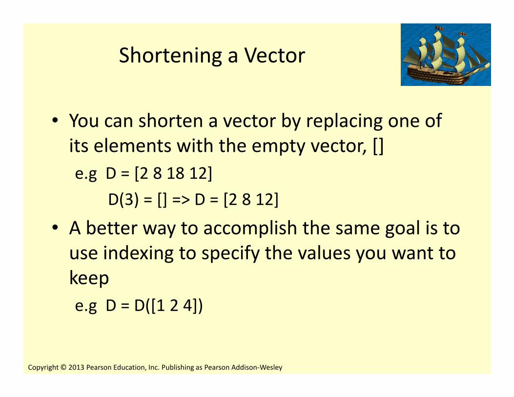
Shortening a Vector

• You can shorten a vector by replacing one of

its elements with the empty vector, []

e.g D = [2 8 18 12]

D(3) = [] => D = [2 8 12]


D(3) = [] => D = [2 8 12]

• A better way to accomplish the same goal is to

use indexing to specify the values you want to

keep

e.g D = D([1 2 4])

Common Functions Used on Vectors

• sum(vec) � gives the sum of all the elements in vec

• mean(vec) � gives the average of the elements in vec

• prod(vec)� gives the product of the elements in vec


• prod(vec)� gives the product of the elements in vec

• sort(vec): the sort function will sort the vector in ascending order unless specified otherwise. It has two outputs: [sorted_vec, indices] = sort(vec);

• The second output is the indices that each element in your sorted vector occupied in the original vector.

More Functions

find(logical)� will return the indices in vec where the element is true.

e.g: vec = [7 3 9 5];

x = find(vec<=7); � x=[1 2 4]

mod(vec, n) � returns the modulus (remainder) of each element in vecdivided by n.

e.g: vec = [4 5 6];


mod(vec, 4) �� [0 1 2]

This function can be used to find even/odd elements in a vector:

x = vec(mod(vec, 2) ~= 0); � finds odds, finds elements in vecthat when divided by 2 do NOT have a remainder of zero! How?

mod(vec, 2) ~= 0 gives us a logical vector [false, true, false], then we used that to index…. vec([false, true, false])….. so it returned the 5 only. The only odd number in our vector. What if we want the index of the odd values?

�find(mod(vec, 2) ~= 0)

3.4 Engineering Example—Forces and

Moments

• Vectors area ideal representations

of the concept of a vector used in

physics.

• Consider two forces acting on an

y

B

C


object at point P, as shown in the

figure.

• Calculate the resultant force at P,

the unit vector in the direction of

the resultant, and the moment

of the force about the point M.

x

z

P

A

M

O

3.4 Engineering Example—Forces and

Moments

y

B

C


x

z

P

A

M

O

Questions?


3.5 Arrays

An array is a rectangular homogeneous collection of data, either

numbers or logical values for now, each of which is called an

element. Each element is located at a row and column of the

array


An example of an array:

A= [1, 2, 3

4, 5, 6];

The array above will be referred to as A2×3

3.5 Arrays

Properties of an ArrayIndividual element in an array are referred to as its elements

The function sz=size(…) will return a vector of length n containing the size of each dimension in an array.


the size of each dimension in an array.

The function length(…) returns the maximum dimension of an array.

The transpose of an m×n array, indicated by apostrophe character (‘), returns an array of n×m dimensions with the rows and column interchanged.

Creating an Array

1. Direct Entry: Just type it in….

X = [1 2 3; 4 5 6]; must be rectangular

Or X = [1 2 3

4 5 6];2. X = zeros(r, c) OR ones(r, c): the inputs are ‘r’ the

number of rows and ‘c’ the number of columns


number of rows and ‘c’ the number of columns

X = zeros(2, 3) � X = [0 0 0

0 0 0];3. X = rand(r, c): generates an array of ‘r’ rows and ‘c’

columns of random numbers between 0 and 1. If you want

a 3*5 array random numbers between 4 and 7:

X = 4 + (7-4)*rand(3, 5)

Building an Array by Concatenation

– HORIZONTAL concatenation:

X = [1; 2; 3]; Y=[4; 5; 6]

XY = [X, Y]; � I used a comma, I didn’t HAVE to, I could just do [X Y]

XY=[1 4

2 5

3 6];


3 6];

– VERTICAL concatenation.

Vert = [X; Y] � vert = [1

2

3

4

5

6];

Accessing and Indexing!

You can access/manipulate several items at once as follows:vec(1,[1 2]) = 0;This would result in : vec = [0 0 0 0

9 0 0 11];

An 'index' refers to a 'spot' in an array or a particular element. i.e.

ar = [3 5; 2 7]

Here ar(2, 2) = 7; ar(1, 2) = 5; and ar(1, 1) = 3;

Accessing Multiple Items:Indexing:


9 0 0 11];

Notice the first two elements have now been switched to zeros. If we wanted to change them to to 6, 4:vec(1, [1 2]) = [6, 4];

Let’s say we want to access the ODD columns of the EVEN rows only, and set them to 99:vec(2:2:end, 1:2:end) = 99;

You can also set elements in such a manner:ar(2,2) = 9;Now, ar = [3 5; 2 9];If you attempt to add an element past the length of the array it will fill all the empty slots leading to it with zeros:ar(3,4) = 11 → ar = [3 5 0 0

2 9 0 00 0 0 11];

Indices in MATLAB start at 1, there is NO index of ZERO!

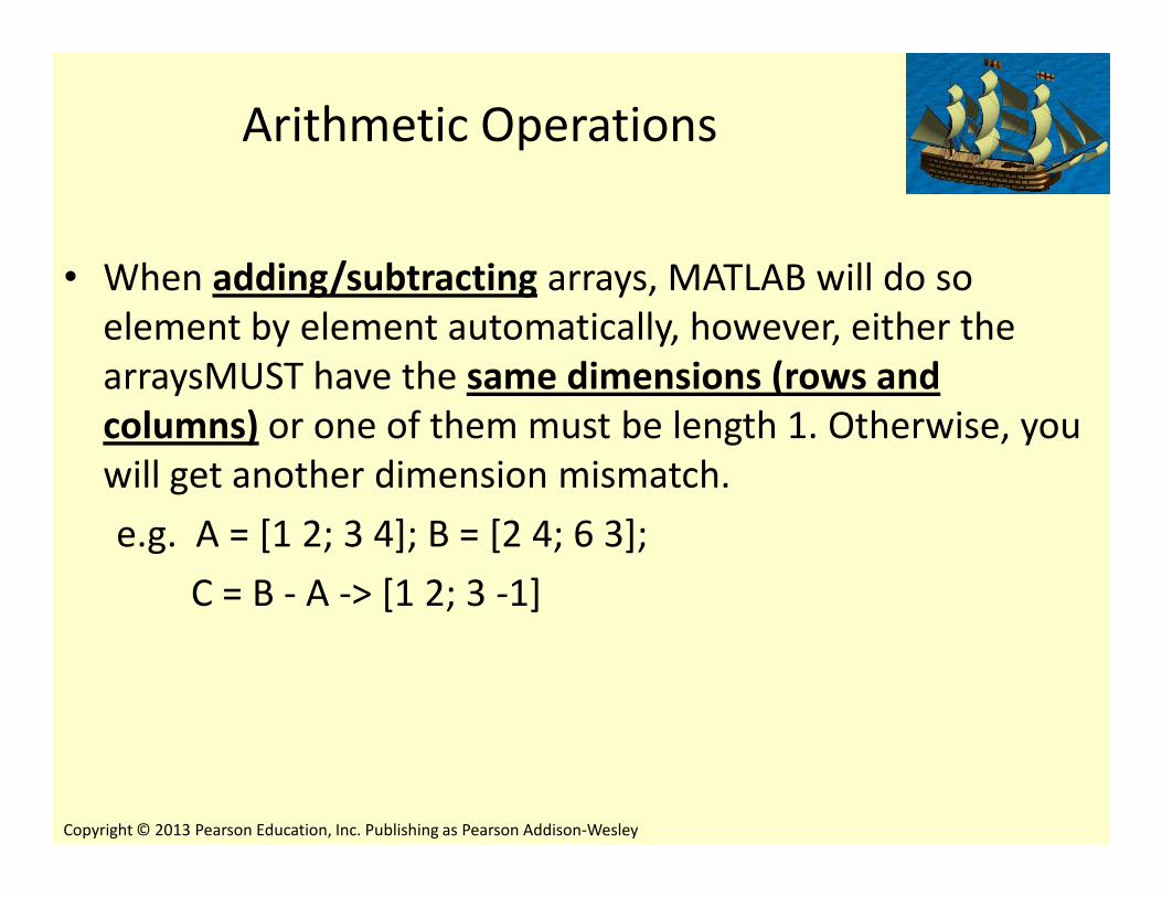
Arithmetic Operations

• When adding/subtracting arrays, MATLAB will do so

element by element automatically, however, either the

arraysMUST have the same dimensions (rows and

columns) or one of them must be length 1. Otherwise, you

will get another dimension mismatch.


columns) or one of them must be length 1. Otherwise, you

will get another dimension mismatch.

e.g. A = [1 2; 3 4]; B = [2 4; 6 3];

C = B - A -> [1 2; 3 -1]

Multiplication and Division

• When multiplying / dividing two arrays you must use the

dot operators .*, ./, .^:

e.g D = A .* B -> [2 8; 18 12]




would result in a matrix multiplication resulting in:

ans = [14 10

30 24]!

• We will learn about matrix operations in a later chapter.

Logical Indexing

if arr = [1 2; 3 1; 2 1];typing vec==1, or vec < 2 into the command window will return : ans = [1, 0; 0, 1; 0, 1]

where 0 stands for false, and 1 stands for true.

What is really odd is the result when you use find on a logical array:


What is really odd is the result when you use find on a logical array:

find(ans) -> [1 4 6]!

[rows cols] = find(ans) -> rows = [1 2 3], cols = [1 2 2]

Shortening an Array

• You can shorten an array by replacing a complete row or column with the empty vector, []

e.g D = [2 8; 1 2; 18 12]


e.g D = [2 8; 1 2; 18 12]

D(2, : ) = [] => D = [2 8; 18 12]

• A better way to accomplish the same goal is to use indexing to specify the values you want to keep

e.g D = D([1 3], :)

Common Functions Used on Arrays

• sum(arr) � gives a vector containing the sum of the elements in each column of arr

• mean(arr) � gives a vector containing the average of the elements in each column of arr

• prod(arr)� gives a vector containing the product of


• prod(arr)� gives a vector containing the product of the elements in each column of arr

• find(logical)� will return the indices in a column vector that is a reshape of the original logical array where the element is true.

e.g: vec = [7 3; 9 5];

x = find(vec<=7); � x=[1 2 4]!!!

Let’s Write some Code …


3.6 Engineering Example

Computing Soil Volume

When digging for foundations for a building, it is necessary to estimate the amount of soil that must be removed. The first step is to survey the land on which the building is to be built, which results in a rectangular grid defining the height of each grid point


The next step is to consider an architectural drawing of the basement of the building.

The total amount of soil to move is then the sum of the individual grid point depths multiplied by the area in each square to be removed.



8.5

9


0

5

10

15

20

0

2

4

6

8

10

12

6

6.5

7

7.5

8



2

4


2 4 6 8 10 12 14 16 18

6

8

10

12



The code in Listing 3.4 produces an answer ~1,120 and we should ask whether this is reasonable.


There are 12x18 squares, each with area 1 unit, about 80% of which are excavated, giving a surface area of about 170 square units. The average depth of soil is about 7 units, so the answer ought to be about 170*7=1,190 cubic units.

This is reasonably close to the computed result.

Homework on Chapter 3 is posted on the website:


http://www.ee.nmt.edu/~erives/289_F12/EE289.html

Homework is due in a week

Chapter 3 Erives - Electrical Engineeringerives/289_F12/Chapter_3_Erives.pdfVectors and arrays are...

Documents

Transcript of Chapter 3 Erives - Electrical Engineeringerives/289_F12/Chapter_3_Erives.pdfVectors and arrays are...