Resilient Human Communities - Social-Ecological Resilience Theory
Ecological Resilience Indicators for Five Northern Gulf of Mexico Ecosystems
91
Chapter 3. Ecological Resilience Indicators for Mangrove Ecosystems
Richard H. Day1, Scott T. Allen2, Jorge Brenner3, Kathleen Goodin4, Don Faber-Langendoen4, Katherine
Wirt Ames5
1 U.S. Geological Survey, Wetland and Aquatic Research Center, Lafayette, LA, U.S.A.
2 ETH Zurich, Department of Environmental Systems Science, Zurich, Switzerland 3 The Nature Conservancy, Texas Chapter, Houston, TX, U.S.A. 4 NatureServe, Arlington, VA, U.S.A. 5 The Nature Conservancy, Gulf of Mexico Program, Punta Gorda, FL, U.S.A.
Ecosystem Description
Mangrove ecosystems are characterized by often flooded saline soil conditions. Three tree species are
commonly found in the Northern Gulf of Mexico (NGoM) mangrove ecosystems: black mangrove
(Avicennia germinans), white mangrove (Laguncularia racemosa), and red mangrove (Rhizophora
mangle). While these species differ in growth form, there can also be substantial plasticity in individuals
within a species, leading to a variety of different forest structures in different hydrogeomorphic
environments. Mangrove ecosystems in the NGoM represent the majority of this ecosystem along the
United States coastline. This is largely due to temperature sensitivity, which results in dramatic dieback
of mangroves where freezing occurs, even periodically. Much of the NGoM is at the latitudinal limit for
mangroves, and mangrove ecosystems in this region can be highly dynamic due to this driving
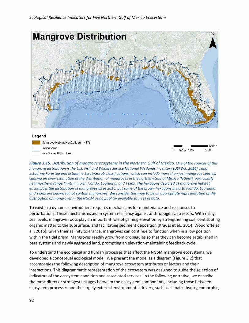
disturbance regime. Figure 3.1 provides a general distribution of mangrove ecosystems in the NGoM.
Numerous independent or interacting factors control the condition, sustainability, and distribution of
mangrove ecosystems. Like other coastal ecosystems, naturally dynamic conditions resulting from
weather patterns drive riverine, estuarine, and coastal hydrogeomorphology and ultimately the spatial
pattern of mangroves (Lugo and Snedaker, 1974). Precipitation gradients restrict the full development of
mangrove ecosystems to relatively humid climates (Osland et al., 2016). Due to their sensitivity to
freezing and regular damage/recovery cycles after freeze events (Osland et al., 2015), climate provides a
major disturbance cycle at the northern limits. Heavily populated coastlines in the region also make
mangroves vulnerable to anthropogenic disturbances such as those to the landscape (channelization,
impoundment), those on soil or water properties (eutrophication, pollution), or those on species
(vegetation planting/removal, burning, introduction of invasive species). People may actively manage to
reduce mangroves where marsh ecosystems are preferred. Sea-level rise further limits their distribution.
Ecological Resilience Indicators for Five Northern Gulf of Mexico Ecosystems
92
Figure 3.15. Distribution of mangrove ecosytems in the Northern Gulf of Mexico. One of the sources of this
mangrove distribution is the U.S. Fish and Wildlife Service National Wetlands Inventory (USFWS, 2016) using Estuarine Forested and Estuarine Scrub/Shrub classifications, which can include more than just mangrove species, causing an over-estimation of the distribution of mangroves in the northern Gulf of Mexico (NGoM), particularly near northern range limits in north Florida, Louisiana, and Texas. The hexagons depicted as mangrove habitat encompass the distribution of mangroves as of 2016, but some of the brown hexagons in north Florida, Louisiana, and Texas are known to not contain mangroves. We consider this map to be an appropriate representation of the distribution of mangroves in the NGoM using publicly available sources of data.
To exist in a dynamic environment requires mechanisms for maintenance and responses to
perturbations. These mechanisms aid in system resiliency against anthropogenic stressors. With rising
sea levels, mangrove roots play an important role of gaining elevation by strengthening soil, contributing
organic matter to the subsurface, and facilitating sediment deposition (Krauss et al., 2014; Woodroffe et
al., 2016). Given their salinity tolerance, mangroves can continue to function when in a low position
within the tidal prism. Mangroves readily grow from propagules so that they can become established in
bare systems and newly aggraded land, prompting an elevation-maintaining feedback cycle.
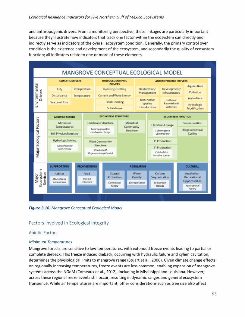
To understand the ecological and human processes that affect the NGoM mangrove ecosystems, we
developed a conceptual ecological model. We present the model as a diagram (Figure 3.2) that
accompanies the following description of mangrove ecosystem attributes or factors and their
interactions. This diagrammatic representation of the ecosystem was designed to guide the selection of
indicators of the ecosystem condition and associated services. In the following narrative, we describe
the most direct or strongest linkages between the ecosystem components, including those between
ecosystem processes and the largely external environmental drivers, such as climatic, hydrogeomorphic,
Ecological Resilience Indicators for Five Northern Gulf of Mexico Ecosystems
93
and anthropogenic drivers. From a monitoring perspective, these linkages are particularly important
because they illustrate how indicators that track one factor within the ecosystem can directly and
indirectly serve as indicators of the overall ecosystem condition. Generally, the primary control over
condition is the existence and development of the ecosystem, and secondarily the quality of ecosystem
function; all indicators relate to one or more of these elements.
Figure 3.16. Mangrove Conceptual Ecological Model
Factors Involved in Ecological Integrity
Abiotic Factors
Minimum Temperatures
Mangrove forests are sensitive to low temperatures, with extended freeze events leading to partial or
complete dieback. This freeze induced dieback, occurring with hydraulic failure and xylem cavitation,
determines the physiological limits to mangrove range (Stuart et al., 2006). Given climate change effects
on regionally increasing temperatures, freeze events are less common, enabling expansion of mangrove
systems across the NGoM (Comeaux et al., 2012), including in Mississippi and Louisiana. However,
across these regions freeze events still occur, resulting in dynamic ranges and general ecosystem
transience. While air temperatures are important, other considerations such as tree size also affect
Ecological Resilience Indicators for Five Northern Gulf of Mexico Ecosystems
94
resilience (Osland et al., 2015). Climate regime determines the permanence of the system, so more
dynamic systems are expected at the latitudinal limits of mangroves (i.e., the northern edge of the
NGoM—North Texas, Louisiana, Mississippi, Alabama, North Florida). Thus, a mangrove system near the
latitudinal limit can still be behaving naturally with frequent mortality, albeit with reduced function
(Cavanaugh et al., 2014; Osland et al., 2013; Saintilan et al., 2014). A similar effect occurs along the
precipitation gradient on the Texas coast with less than optimum mangrove growing conditions along
the arid coast nearing Mexico (Osland et al., 2014; Gabler et al., 2017; Feher et al., 2017).
Soil Physicochemistry
The physical and chemical properties of mangrove soils relate to the hydrologic and geomorphic setting.
Topography and hydrologic regime (including water quality) determine deposition patterns, ultimately
determining where and how much accretion occurs. Proximity to development also provides a major
control on soil composition and how soils develop and change. Mangroves, like other wetlands, are
characterized by soils with low oxygen levels due to frequent inundation.
Although hypoxia can generally inhibit primary production and soil microbial processes, mangroves are
adapted to hypoxic conditions by being able to oxidize the rhizosphere. More importantly, frequent tidal
flushing maintains higher dissolved oxygen concentrations than seen in impounded wetlands, which
may have critically low oxygen concentrations (Mitsch and Gosselink, 2015). Decomposition of organic
matter can and does also occur through anaerobic respiration pathways, facilitating energy flow through
the detrital community. However, restrictions to tidal flushing result in dramatically reduced function
due to limitations on dissolved oxygen (Lewis et al., 2016).
Salinity is a dominant feature of soil physicochemistry, excluding other species and thereby enabling the
dominance of mangrove species. While mangroves tolerate high salinities, excess salinity can produce
stressful conditions, particularly in basin mangrove systems where salinities can become hypersaline.
Hypersalinity occurs in areas not connected to coastal fluxes, such that isolated areas become
increasingly saline with evaporation. In contrast, isolated areas can also become increasingly fresh
where and when precipitation is more frequent.
Mangrove ecosystems that are connected to estuaries and rivers generally have soils that have a higher
nutrient and mineral content. Nutrient limitations can occur where there are only oceanic influences
and terrigenous sediment inputs are minimal (e.g., biogenic wetlands on top of carbonate platforms as
in South Florida) (Feller, 1995). The presence of mineral content shows an external deposition source
that can aid in maintaining elevations and results in higher bulk density (Morris et al., 2016). Lower
organic matter can indicate greater resistance to change because components are less likely to leave as
dissolved lateral fluxes. Elevated nutrients, while potentially increasing plant production, are not
necessarily optimal for system sustainability (Lovelock et al., 2009). Nutrient enrichment can increase
aboveground production (leaves, stems) with simultaneous decreases to belowground production. A
resulting lower root-to-shoot ratio can lead to mortality (Lovelock et al., 2009) and likely more erosion
and elevation loss from reduced root strength.
Hydrologic Setting
Hydrologic setting incorporates precipitation patterns, connectivity to the ocean, connectivity to rivers,
elevation, water table variability, sea level rise, water chemical composition, and many other factors.
While all certainly have some effects on mangrove ecosystems, connectivity and hydrologic exchanges
Ecological Resilience Indicators for Five Northern Gulf of Mexico Ecosystems
95
are prominently important. Mangroves exist in different geographic positions, which are associated with
different hydrologic environments (Lugo and Snedaker, 1974; Mitsch and Gosselink, 2015). Fringe
mangroves occupy coastal boundaries with frequent inundation, and water levels are almost exclusively
driven by tide (most connected to ocean). Riverine mangroves occupy riparian zones along coastal
channels and tidal creeks (less connected). Basin mangroves occupy inland depressions or impounded
areas resulting in partially or fully stagnant water (least connected). Two other physiognomic settings of
mangroves occur in overwash zones (high wave energy and/or tidal velocities) and dwarf or scrub
forests (nutrient limited and/or hypersaline) (Lugo and Snedaker, 1974).
Often wetland water level variability is characterized by ‘hydroperiod’ incorporating flood depth,
duration, and frequency, and the variability surrounding those parameters. However, the most
important factor for mangroves is the degree of water exchange versus stagnancy. Lower elevation may
be more vulnerable to submergence, and low elevation with exchange yields conditions that are more
habitable than hypersaline disconnected areas. For low elevation to be sustainable and the hydrologic
regime to be stationary (relative to elevation), sea-level rise must be matched by elevation gain.
Connectivity has many definitions, but here we use it to describe the ease of flow of matter. Low
connectivity results in little water level variability, hypoxia, often hypersaline or fresh conditions
(depending on climate), and accumulation of other chemicals. High connectivity areas have a chemical
composition and water level pattern that mimics surrounding bodies of water, typically resulting in
salinities and nutrient levels similar to adjacent aquatic environments. Altered connectivity (e.g., by
construction of berms or diverted flows) can result in rapid decline and potentially complete mortality,
because mangroves are stressed by anoxic and/or hypersaline conditions (Lewis et al., 2016). This can
also result in degradation of associated communities (e.g., microbes and fish).
Water quality is affected by many of the factors that also influence hydrologic variability. The
geomorphic setting determines water sources (Brinson, 1993) and ultimately the constituents within
that water. Important components of water quality in mangroves are salinity, total suspended solids
(TSS), and nutrient load—particularly those nutrients contributing to eutrophication. These same three
factors are necessary elements of mangrove ecological function, but can become stressors to the system
at higher concentrations. Human activity can directly and indirectly influence quality through system
modifications. For example, dams and levees alter flow velocity and therefore how much sediment exits
a river system (Tockner et al., 1999). Agricultural activity generally increases nutrients loads, increasing
the likelihood of eutrophication.
Ecosystem Structure
Plant Community Structure
Mangrove ecosystems exist with a diversity of structures that arise from land history, abiotic conditions,
and the species present. Prominent physical characteristics defining mangrove systems are a dense
canopy with highly intertwined crowns, frequently an understory dominated by prop roots, and a
ground surface that is regularly flooded, with microbial mats, pneumatophores (extending from
mangrove roots), or salt marsh grasses and forbs. Otherwise the understory can be remarkably bare
(Mitsch and Gosselink, 2015).
Ecological Resilience Indicators for Five Northern Gulf of Mexico Ecosystems
96
Tree growth forms vary both within and across species, generally ranging from low shrubs to tall trees.
Fringe and overwash systems tend to have mostly red mangroves; basin mangrove forests are
dominated by black mangroves and white mangroves; and riverine and dwarf/scrub forests have
mixtures of all three species. Riverine forests have generally taller and larger trees compared to basin
and scrub mangroves, which are dominated by smaller and less dense individuals (Lugo and Snedaker,
1974; Day et al., 1989; Mitsch and Gosselink, 2015). All of these physiognomic patterns are mediated by
the climate of the geographic location within the NGoM; freezing winter temperatures will have species
specific effects of dieback, which can result in a scrub form (McMillan and Sherrod, 1986; Day et al.,
2013). Black mangroves are the most freeze-tolerant and thus dominate the extreme northern latitudes
of the NGoM, regardless of hydrologic setting (Day et al., 2013). Given that these trees are long-lived,
these size relationships are also a function of site permanence as opposed to just growth and production
rates; for large trees to occur, the ecosystem must be stable enough to maintain adequate growing
conditions over a long duration.
Viability of propagules and saplings vary by site biotic and abiotic conditions. Optimal conditions for
sapling growth are generally below ocean salinities (3–27 PSU), temperatures well below physiological
limits, with gaps and thus available light; however, results are variable among studies (Krauss et al.,
2008). It is likely that, like most plant ecosystems, establishment relies upon the availability of
propagules, availability of growing space, and appropriate conditions that do not appear particularly
distinct from those where overstory mangroves exist. The ability to successfully establish from
propagule (Delgado et al., 2001) does enable development of new mangrove systems.
Landscape Structure
Despite low species diversity, morphology of the mangrove landscape can be very complex due to
geographic setting, with secondary effects from the competing factors of deposition and erosion, both
of which are affected by both ecological and anthropogenic factors. Mangroves expand through
dispersal of floating propagules, and hydrology plays a key role in the rate of expansion as well as the
relation of hydrologic barriers to landscape structure. Mangroves can expand into systems other than
mudflats if conditions change to favor mangroves or if mangroves simply outcompete marsh vegetation.
Like marshes, landscape change in mangrove ecosystems can also occur through lateral erosion and
migration (Fagherazzi et al., 2013), which may occur in rapid pulses from storm influences
(Guntenspergen et al., 1995; Smith et al., 2009). While mangroves can exist in large expansive areas,
internal basins receive increasingly less exchange, which ultimately leads to dieback of internal areas
(Lewis et al., 2016). Internal die back leads to a more disaggregated landscape (i.e., greater edge-to-area
ratio).
Human effects on landscape structure are prominent. Indirect anthropogenic effects on landscape
patterns include upstream control over the transport of sediment and nutrients (Kennish, 2001). Even if
infrastructure development does not directly remove mangroves, modifications to the environment can
have significant effects on habitat connectivity. Depending on the type and nature of infrastructure
present, it may directly affect water and material flow, produce a barrier to plant and/or animal
migration, and contribute to habitat fragmentation. The development of channels can alter water and
sediment flows into and out of mangrove forests, as well as alter species corridors (Turner, 2010). Oil
removal can directly drive subsidence (Kennish, 2001), and unintentional releases of petrochemicals can
alter geomorphic stability (DeLaune et al., 1979). Reduced or absent vegetation, whether impaired by
Ecological Resilience Indicators for Five Northern Gulf of Mexico Ecosystems
97
petrochemicals (Culbertson et al., 2008) or other processes, results in less protection of surface
sediments from erosive forces (Kadlec, 1990).
Microbial Community Structure
Mangrove microorganisms include fungi, bacteria, and other species that occupy the rhizosphere and
litter layers. Microbial mats on the soil surface can be particularly high in productivity (Zedler, 1981) and
play an important role in total ecosystem function. Subsurface processes maintain elevation and provide
the organic effluxes that provide an energy source for landscape-level productivity. Studies have shown
that coastal soil microbial communities, or at least the fluxes they control, can be fairly resilient against
pollution effects (DeLaune et al., 1979; Li et al., 1990), although changes may alter respiration and other
processes (Chambers et al., 2013).
Ecosystem Function
Elevation Change
Elevation change is an essential function for the sustainability of mangrove ecosystems because sea
levels change and land subsides. Interpretation of elevation change should be placed in the context of
initial elevation relative to sea level, sea-level change, and tidal range. Decreases in elevation relative to
sea level occur with sea-level rise and surface erosion and subsidence, which is influenced by erosion,
decomposition, and compaction of sediments (Cahoon and Turner, 1989), subsurface withdrawals (e.g.,
water, oil, gas) and geologic activity (Kennish, 2001). Elevation gains occur by sediment deposition and
in situ biomass production contributing to organic accretion (from leaves, roots, exudates, and soil
biota). Slow decomposition rates associated with mangrove biomass can be important to maintaining
peat accumulation that contributes to elevation capital (McKee et al., 2007).
Elevation and sea level change have feedback because organic accumulation and sedimentation rates
are dependent on tidal flooding and the relative elevation within the tidal range. Accordingly, areas with
a smaller tidal range, such as those in the NGoM, are more vulnerable to sea-level rise. While this
concept has mostly been explored in salt marshes (e.g., Kirwan and Megonigal, 2013), the same
processes occur in mangroves. Spring tidal ranges in the Gulf vary from approximately 0.3 m in south
Texas to 1 m in south Florida, whereas elsewhere on the Atlantic and Pacific coasts, tidal ranges vary
from 1 to > 3 m (Tiner, 2013). Despite high productivity in the NGoM region (Kirwan et al., 2009), total
accretion rates are generally low (Neubauer, 2008) because of the small tidal range and small
allochthonous sediment supply.
Primary Production
Primary production varies by system type, with higher productivity in fringe and riverine systems
(Mitsch and Gosselink, 2015). Overall, mangroves are high productivity systems (10–30 Mg ha-1 yr-1
(Bouillon et al., 2008), comparable to other forest systems in tropical regions (e.g., biome mean of
tropical rain forest aboveground net primary productivity = 1.4 Mg ha-1 yr-1; Chapin et al., 2002). While
these values are not well constrained and are considerably uncertain, the potentially high production is
noteworthy because of its contribution towards elevation gains.
Controls over productivity are not well understood, but salinity, phosphorus, nitrogen, and hydroperiod
appear to have important effects (Feller et al., 2003; Feller et al., 2007; Krauss et al., 2006; Scharler et
al., 2015), but with optimal conditions being more intermediate. In general, phosphorus is limiting on
Ecological Resilience Indicators for Five Northern Gulf of Mexico Ecosystems
98
carbonate substrates, and nitrogen is limiting in areas that receive high sediment inputs (Feller et al.,
2007; McKee et al., 2002). Climate is an important control, with lower latitudes having higher
productivity. Understanding of productivity is limited by very few measurements of wood production
and even fewer estimates of root production (Bouillon et al., 2008). However, impeded connectivity is a
stressor (Lewis et al., 2016) and associated conditions (low dissolved oxygen, low matter exchange, and
high salinity) reduce productivity (Gilman et al., 2008). These effects are exacerbated by lower
precipitation amounts that can further increase salinity and force early senescence (e.g., Day et al.,
1996).
Decomposition
Besides the importance of decomposition to elevation changes, secondary production largely relies on
decomposition (herbivores use a small fraction of live biomass) and the organic exports, which can be
particularly high in mangroves (Maher et al., 2013). However, the high tannin content of partially
decomposed mangrove materials may be less ideal for macrofaunal consumption (Lee, 1985). This is a
primary difference from marsh ecosystems, where decomposition largely takes place in the marsh and is
thus exported as more readily consumable products (Lee, 1985). Decomposition rates vary
tremendously by species, plant component, and ecosystem, with more impounded areas generally
having slower decay rates (and, therefore lower DOC and DIC exchange rates).
Secondary Production
Secondary production in mangroves is mostly composed of soil microbial processes, with their biological
activity most easily monitored through soil respiration measurements, which are largely driven by soil
temperatures (e.g., Lovelock, 2008). Besides the microbial community, crabs are abundant; however,
they do not necessarily play an important role in leaf decomposition as observed elsewhere (McIvor and
Smith, 1995).
Bird and fish communities are apparent. The dense ecosystem structure provides important nursery
habitat for many species. Due to the southern extent of mangroves into tropical Florida, several species
that are rare or absent from the rest of the United States are found in mangrove ecosystems (mangrove
cuckoo, white crowned pigeon) (Bird Watcher’s Digest, 2017). Likewise, southern mangrove systems are
vulnerable to species invasion by tropical species—an abundance of invasive species are currently in
mangroves in southern Florida (Fourqurean et al., 2010; Ward et al., 2016).
Management considerations that negatively affect the trees and their production have cascading effects
on the heterotrophic communities. Conditions that lower tree productivity also alter the availability of
energy sources to other trophic levels. Furthermore, the physical impediments to connectivity that
stress trees also limit the exchange of matter and biota between mangrove forests and the surrounding
aquatic environment (Lewis and Gilmore, 2007).
Biogeochemical Cycling
Biogeochemical cycles are inexorably involved in all factors discussed above because of the chemical
transformations and exchanges that occur. Nitrogen cycles are especially distinct in wetlands because of
the presence of both oxic and anoxic conditions, enabling nitrification and subsequent denitrification. In
areas where nitrogen is unnaturally elevated, nitrogen cycling in wetlands can play an important role in
reducing eutrophication (Mitsch and Gosselink, 2015).
Ecological Resilience Indicators for Five Northern Gulf of Mexico Ecosystems
99
The accretion of nutrient-rich sediments in wetlands can allow for storage of nutrients, removing a
portion from circulation. Accordingly, the conditions that allow these long-term capture, storage, or
transformation are essential to elevation maintenance because they are part of the stabilization of
sediments required for vertical accretion; that is, pedogenesis results in more stability than
disaggregated sediments would otherwise have.
Mangroves play an atypical role in the greenhouse gas budget where salinity and water level variations
can occur such that they can act as a carbon sink (through production and storage) or as a carbon
source, due to effluxes of CO2, CH4, and nitrous oxide (e.g., Chen et al., 2016), which alter atmospheric
chemistry and radiative forcing. In general, healthy mangrove ecosystems in a stable tidal regime can
sequester carbon, but factors which degrade or cause mortality of mangroves can lead to carbon
release.
Factors Involved in Ecosystem Service Provision
Mangrove forests constitute one of the most productive ecosystems in the world, providing a diverse
suite of ecosystems services upon which human well-being depends. These unique forests exist both
above and below the waterline, providing habitat for an exceptional suite of biodiversity, including many
threatened species. They provide fish habitat and nursery areas which support subsistence and
commercial production while also providing timber, wood and medicinal plants. The physical structure
of mangrove ecosystems acts to stabilize shorelines and protect vulnerable coasts from wind and wave
erosion. Several studies have analyzed the value of mangroves and other habitats for protection of
coastal communities from storm surge (e.g., Barbier et al., 2008; Costanza et al., 2008; Das and Vincent,
2009). It is often difficult to be precise about how much protection ecosystems are likely to provide
given the variability of storms, including wind speed and direction, duration, and arrival of the storm
relative to high tides (Koch et al., 2009), but there can be little doubt that their contributions can be
significant. These protection benefits reduce the risk of human and material losses, thus enhancing
economic benefits by upholding the diverse functions and uses of mangrove ecosystems, including
potential biodiversity-related tourism (UNEP, 2014; Danielsen et al., 2005).
Globally, mangrove forests and estuaries provide environmental services that mitigate and facilitate
adaption to climate change, as they not only reduce the risks of extreme weather events, but also have
great potential to sequester and store carbon (Twilley et al., 1992; Donato et al., 2011; Coastal Blue
Carbon, 2015; Barbier et al., 2011). A complete list of the services provided by mangroves in the NGoM
is provided by Yoskowitz et al. (2010); below we provide an overview of the most important Key
Ecosystem Services that we included in the conceptual ecological model.
Supporting
Habitat
Mangrove vegetation provides habitat to support the diversity of terrestrial and marine invertebrates
and vertebrates. The mangrove forest provides habitat characteristics that many species depend on,
including good water quality, moderate slope in banks, slow currents, overhanging vegetation that
provides shade, and the structure and protection that is provided by the mangrove shoot and root
systems (Seaman and Collins, 1983). The ability of the mangrove to provide habitat for commercially
Ecological Resilience Indicators for Five Northern Gulf of Mexico Ecosystems
100
important species depends on the factors described for the “Secondary Production” Key Ecological
Attribute above.
Provisioning
Food
Mangroves are the breeding and nursery grounds for many fish species. Ninety percent of the
commercial species in South Florida are dependent on mangrove ecosystems (Law and Pywell, 1988).
Regulating
Coastal Protection
Mangroves provide ecosystem benefits that reduce coastal risks, such as coastal erosion, wave energy
reduction, and storm surge reduction (McIvor et al., 2012). Mangroves help stabilize the shoreline by
reducing the erosion and therefore making the shoreline less vulnerable to other natural hazards (The
Nature Conservancy, 2017). This is especially important as sea level rises due to climate change, and our
coasts become more vulnerable in places where marshes are not present or are threatened (TNC and
NOAA, 2011). The protection benefit of any mangrove vegetation will depend on many factors, such as
exposure, intensity, and local conditions.
Reduction of wave energy depends on the structure of the plant canopy, its height and density, and the
cross-shore and along-shore extent of the wetland (Koch et al., 2009; Krauss et al., 2009; Massel et al.,
1999; Narayan and Kumar, 2006; Shepard et al., 2011; Vosse, 2008). The velocity of water traveling
within a plant canopy is relatively lower than above the canopy. Canopy height in relation to water
depth is relevant because water flowing through the vegetation encounters a higher friction than does
the water above the vegetation. Therefore, the total friction in the water column will change with the
depth of vegetated and non-vegetated areas. Because a mangrove canopy is taller and exerts more drag
than a salt marsh community, mangroves are more effective at reducing water inflow and waves than
are salt marshes. Quartel et al. (2007) suggested that the drag force exerted by a mangrove forest can
be approximated by the function CD = 0.6e0.15A, where CD is the coefficient of drag and A is the
projected cross-sectional area of the submerged canopy. For the same muddy surface without
mangroves, the drag is a constant 0.6. Mazda et al. (1997) observed that a 100-m-wide strip of
mangrove forest was capable of reducing wave energy by 20 percent. Reduction in water levels across a
mangrove area in Florida was 9.4 cm/km (Krauss et al., 2009).
Water Quality
Mangroves improve water quality by retaining sediment particles and pollutants. Mineral accretion is
important to long-term mangrove sustainability and is dependent on flood regime and the availability of
mineral sediments in the water column (Childers and Day, 1990). While soil organic matter content
reflects some aspects of total suspended solids, it is not directly related due to variations in
hydrogeomorphic position (Hatton et al., 1983). Sediment sources are highly correlated to river delta
morphology and river discharge, but these sources are altered by anthropogenic activity (e.g., levees
and dams; Kennish, 2001).
Ecological Resilience Indicators for Five Northern Gulf of Mexico Ecosystems
101
Carbon Sequestration
Due to high above- and belowground productivity and minimal decomposition, mangroves are capable
of storing large amounts of organic carbon. As such, they play an important role in mitigating climate
change despite their relatively small footprint.
Cultural
Aesthetics-Recreational Opportunities
As nursery grounds for important game fish, mangroves provide opportunities for recreational fishing.
Indicators, Metrics, and Assessment Points
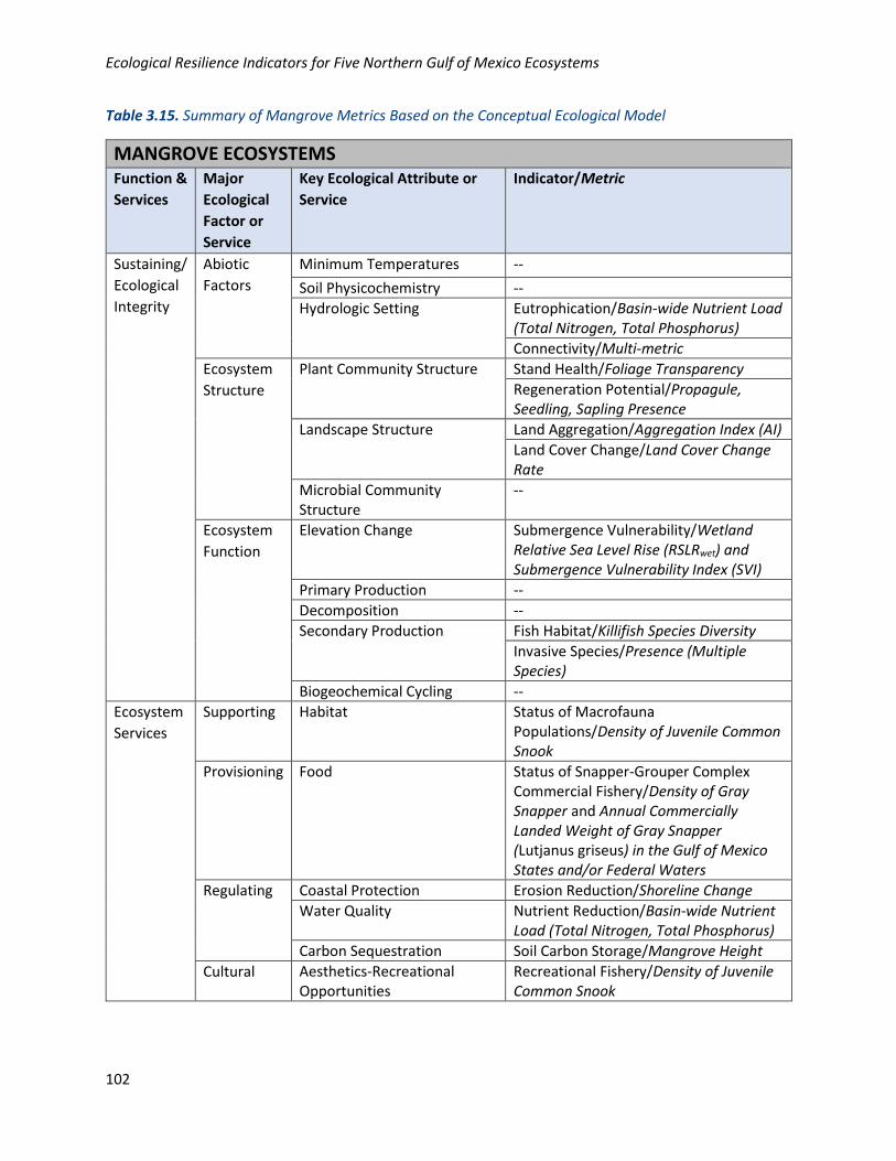
Using the conceptual model described above, we identified a set of indicators and metrics that we
recommend be used for monitoring mangrove ecosystems across the NGoM. Table 3.1 provides a
summary of the indicators and metrics proposed for assessing ecological integrity and ecosystem
services of mangrove ecosystems organized by the Major Ecological Factor or Service (MEF or MES) and
Key Ecological Attribute or Service (KEA or KES) from the conceptual ecological model. Note that
indicators were not recommended for several KEAs or KESs. In these cases, we were not able to identify
an indicator that was practical to apply based on our selection criteria. Below we provide a detailed
description of each recommended indicator and metric(s), including rationale for its selection, guidelines
on measurement, and a metric rating scale with quantifiable assessment points for each rating.
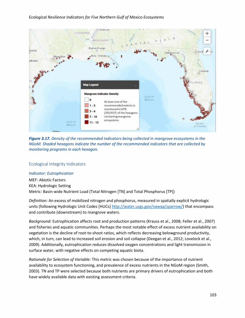
We also completed a spatial analysis of existing monitoring efforts for the recommended indicators for
mangrove ecosystems. Figure 3.3 provides an overview of the overall density of indicators monitored.
Each indicator description also includes a more detailed spatial analysis of the geographic distribution
and extent to which the metrics are currently (or recently) monitored in the NGoM, as well as an
analysis of the percentage of active (or recently active) monitoring programs that are collecting
information on the metric. The spatial analyses are also available in interactive form via the Coastal
Resilience Tool (http://maps.coastalresilience.org/gulfmex/) where the source data are also available for
download.
Ecological Resilience Indicators for Five Northern Gulf of Mexico Ecosystems
102
Table 3.15. Summary of Mangrove Metrics Based on the Conceptual Ecological Model
MANGROVE ECOSYSTEMS Function &
Services
Major
Ecological
Factor or
Service
Key Ecological Attribute or
Service
Indicator/Metric
Sustaining/
Ecological
Integrity
Abiotic
Factors
Minimum Temperatures --
Soil Physicochemistry --
Hydrologic Setting Eutrophication/Basin-wide Nutrient Load (Total Nitrogen, Total Phosphorus)
Connectivity/Multi-metric
Ecosystem
Structure
Plant Community Structure Stand Health/Foliage Transparency
Regeneration Potential/Propagule, Seedling, Sapling Presence
Landscape Structure Land Aggregation/Aggregation Index (AI)
Land Cover Change/Land Cover Change Rate
Microbial Community Structure
--
Ecosystem
Function
Elevation Change Submergence Vulnerability/Wetland Relative Sea Level Rise (RSLRwet) and Submergence Vulnerability Index (SVI)
Primary Production --
Decomposition --
Secondary Production Fish Habitat/Killifish Species Diversity
Invasive Species/Presence (Multiple Species)
Biogeochemical Cycling --
Ecosystem
Services
Supporting Habitat Status of Macrofauna Populations/Density of Juvenile Common Snook
Provisioning Food Status of Snapper-Grouper Complex Commercial Fishery/Density of Gray Snapper and Annual Commercially Landed Weight of Gray Snapper (Lutjanus griseus) in the Gulf of Mexico States and/or Federal Waters
Regulating Coastal Protection Erosion Reduction/Shoreline Change
Water Quality Nutrient Reduction/Basin-wide Nutrient Load (Total Nitrogen, Total Phosphorus)
Carbon Sequestration Soil Carbon Storage/Mangrove Height
Cultural Aesthetics-Recreational Opportunities
Recreational Fishery/Density of Juvenile Common Snook
Ecological Resilience Indicators for Five Northern Gulf of Mexico Ecosystems
103
Figure 3.17. Density of the recommended indicators being collected in mangrove ecosystems in the NGoM. Shaded hexagons indicate the number of the recommended indicators that are collected by monitoring programs in each hexagon.
Ecological Integrity Indicators
Indicator: Eutrophication
MEF: Abiotic Factors
KEA: Hydrologic Setting
Metric: Basin-wide Nutrient Load (Total Nitrogen [TN] and Total Phosphorus [TP])
Definition: An excess of mobilized nitrogen and phosphorus, measured in spatially explicit hydrologic
units (following Hydrologic Unit Codes [HUCs] http://water.usgs.gov/nawqa/sparrow/) that encompass
and contribute (downstream) to mangrove waters.
Background: Eutrophication affects root and production patterns (Krauss et al., 2008; Feller et al., 2007)
and fisheries and aquatic communities. Perhaps the most notable effect of excess nutrient availability on
vegetation is the decline of root-to-shoot ratios, which reflects decreasing belowground productivity,
which, in turn, can lead to increased soil erosion and soil collapse (Deegan et al., 2012; Lovelock et al.,
2009). Additionally, eutrophication reduces dissolved oxygen concentrations and light transmission in
surface water, with negative effects on competing aquatic biota.
Rationale for Selection of Variable: This metric was chosen because of the importance of nutrient
availability to ecosystem functioning, and prevalence of excess nutrients in the NGoM region (Smith,
2003). TN and TP were selected because both nutrients are primary drivers of eutrophication and both
have widely available data with existing assessment criteria.
Ecological Resilience Indicators for Five Northern Gulf of Mexico Ecosystems
104
Annual mean TN and TP concentrations are appropriate for assessment metrics because nutrient fluxes
vary at multiple spatial and temporal scales. Therefore, point measurements in space and time do not
accurately represent the overall ecosystem condition with regard to nutrient cycling. Thus, a spatially
and temporally aggregated metric is preferable for monitoring eutrophication. The HUC scale is the most
readily available aggregated measure available at spatial and temporal scales relevant to ecosystem
condition trends.
Measures: Total phosphorus in mg L-1 and total nitrogen in mg L-1 (basin-wide)
Tier: 1 (remote sensing and modeling)
Measurement: SPARROW (Spatially-Referenced Regression on Watershed Attributes) is a model that
estimates basin-level long-term average fluxes of nutrients (Preston et al., 2011). The model integrates
monitoring site data at high temporal resolution to develop site rating curves (integrating streamflow
and water quality data), which are then extrapolated to individual basins with values scaled by land
classifications within basins. The user-friendly online interface allows determination of both TN and TP
loads for specific basins to identify relative water quality fluxes.
Metric Rating and Assessment Points:
Metric Rating Basin-wide Nutrient Load (mg L-1)
Excellent TP < 0.1 and TN < 1.0 mg
Good TP 0.1–0.2 and TN 1.0–2.0
Fair TP 0.2–0.9 and TN 2.0–7.0
Poor TP > 0.9 and TN > 7
Scaling Rationale: SPARROW outputs for TN concentration range from near 0.05 to > 7 mg L-1 in coastal
basins of the NGoM. TP concentrations range from near 0.00 to > 0.9 mg L-1 in coastal basins of the
NGoM. Applying these criteria to mangrove ecosystems necessarily takes into account that mangroves
grow in varying steady-state morphological forms (gallery forests in riverine areas to dwarf forests on
carbonate substrates in the Florida Keys). While low nutrient concentrations do not necessarily indicate
superior ecological function for all aspects of the ecosystem, the potential for eutrophication in soils and
within the water column declines with lower nutrient concentration values. Assessment points were
established in accordance with the SPARROW output breakpoints for mapping convenience; groupings
were established to flag higher values as fair or poor. These higher values are in ranges generally
associated with impaired water quality. Of the NGoM states, only Florida has state-specific criteria (e.g.,
0.4 to 1 mg L-1 TN, depending on specific estuary; US EPA, 2016).
Analysis of Existing Monitoring Efforts:
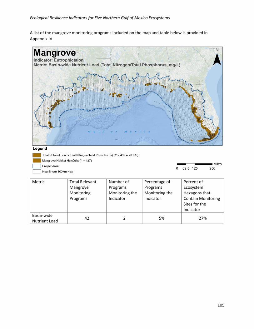
Geographic: Basin-wide nutrient load is moderately well collected geographically in the NGoM, with 27%
of habitat hexagons containing at least one monitoring site. Monitoring locations for this metric are
relatively well distributed across the NGoM where mangroves occur.
Programmatic: Data for this metric are collected by 2/42 (5%) of the programs collecting relevant
mangrove data in the NGoM.
Ecological Resilience Indicators for Five Northern Gulf of Mexico Ecosystems
105
A list of the mangrove monitoring programs included on the map and table below is provided in
Appendix IV.
Metric Total Relevant Mangrove Monitoring Programs
Number of Programs Monitoring the Indicator
Percentage of Programs Monitoring the Indicator
Percent of Ecosystem Hexagons that Contain Monitoring Sites for the Indicator
Basin-wide Nutrient Load
42 2 5% 27%
Ecological Resilience Indicators for Five Northern Gulf of Mexico Ecosystems
106
Indicator: Connectivity
MEF: Abiotic Factors
KEA: Hydrologic Setting
Metric: Multi-metric
Definition: The ease of water flow into and out of a site.
Background: Where connectivity is impaired, issues such as hypoxia and hyper-salinity affect forest
health. These impacts are arguably more prevalent to aquatic communities affected by changing water
quality. Connectivity impairment manifests in quantitative and qualitative changes to hydrologic
variability and water chemistry that can be detected. As mangrove stands lose hydrologic connectivity
and become more stagnant, dissolved oxygen levels decrease, salinity increases, standing water in the
stand builds up tannins, and sulfate-reducing bacteria become visibly apparent (anaerobic bacteria
indicative of anoxic conditions [Day et al., 1989]). Because connectivity impairment is not likely in a
fringe mangrove system, this assessment only applies to basin mangroves.
Rational for Selection of Variable: In the absence of hydrologic connectivity, there are rapid
consequences that alter the biogeochemical and physiological processes that can lead to mortality and
change of the ecosystem entirely.
Measure: (a) relative tidal signature | (b) water color | (c) dissolved oxygen (DO) level | (d) sulfate-
reducing bacteria | (e) salinity | (f) observable presence of flow barriers
Tier: 2 (rapid field measurement) and 3 (intensive field measurement)
Measurement: Multiple assessment approaches are offered because sites differ in logistical ease of
access. With proper equipment, salinity, dissolved oxygen, and water level variability are all easily
measured. With experience, connectivity may be assessed by simple observations of water color,
presence of bacterial films, or presence of obvious flow barriers. Although six metrics are described (a–
f), one metric should be chosen due to ease of measurement, or observer expertise, and followed
through all three ratings, rather than using a different metric for each rating.
Metric Rating and Assessment Points:
Metric Rating Connectivity Multi-metric
Excellent–Good (a) sinusoidal tidal signature mirroring connected body of water, (b) water has color expected based on nearby water bodies, (c) DO varies with tide, (d) bacterial films are not apparent, (e) salinity >10 PSU and < 45 PSU, depending on location of mangroves with relation to freshwater input (f) no apparent obstructions to flow
Fair (a) some tidal variability apparent, but not following reference pattern, (b) reddish brown colored water (c) DO < 2 mg/L (hypoxic) under restricted flow condition, (d) sulfate reducing bacterial films may be present in small non-draining pools, (e) PSU > 45 or PSU < 90 (f) flow barriers restricting flow (e.g., road with undersized culvert)
Poor (a) no tidal signature, (b) dark brown to black colored water, (c) DO near 0 mg/L (anoxic) under chronic stagnant condition, (d) bacterial films are widespread (e) PSU > 90 (f) berm around site or tidal channel filled, cutting off all flow

Ecological Resilience Indicators for Five Northern Gulf of Mexico Ecosystems
107
Scaling Rationale: Measurement of a tidal signature within a mangrove stand that is similar to the
connecting body of water outside the stand is direct evidence of water flow in and out of the stand.
Attenuation to absence of the tidal signature (caused by berms or tidal channel filling) indicates
restricted to no flow, respectively. With restricted or absence of flow, water color becomes more tannic
as stagnation ensues. Flow from a connecting body of water imparts oxygenated water to a mangrove
stand. NOAA has defined hypoxia in the NGoM as water where the DO concentration is less than 2 mg/L
(https://www.ncddc.noaa.gov/hypoxia/). While mangroves are adapted to survive in hypoxic and
hypersaline conditions (Mitsch and Gosselink, 2015), it is not the optimum for highest mangrove growth
and productivity. While mangroves may survive in conditions of PSU > 90, optimum growth of some
species is about half of seawater (Tomlinson, 1986). Seawater averages about PSU 35
(http://oceanservice.noaa.gov/facts/whysalty.html). Sulfate-reducing bacterial films indicating anoxic
conditions are easily visible to a trained eye.
Analysis of Existing Monitoring Efforts:
Geographic: The metrics that are used to assess connectivity are collectively well collected
geographically in the NGoM, with 51% of habitat hexagons containing at least one monitoring site for at
least one of the metrics. Monitoring locations for these metrics are well distributed across the NGoM
where mangroves occur.
Programmatic: Data for this metric are collected by 9/42 (21%) of the programs collecting relevant
mangrove data in the NGoM.
A list of the mangrove monitoring programs included on the map and table below is provided in
Appendix IV.
Ecological Resilience Indicators for Five Northern Gulf of Mexico Ecosystems
108
Metric Total Relevant Mangrove Monitoring Programs
Number of Programs Monitoring the Indicator
Percentage of Programs Monitoring the Indicator
Percent of Ecosystem Hexagons that Contain Monitoring Sites for the Indicator
Connectivity Multi-metric
42 9 21% 51%
Ecological Resilience Indicators for Five Northern Gulf of Mexico Ecosystems
109
Indicator: Stand Health
MEF: Ecosystem Structure
KEA: Plant Community Structure
Metric: Foliage Transparency
Definition: Relative assessment of the amount of light penetrating the tree canopy.
Background: A mangrove forest stand losing foliage cover is a sign of unhealthy conditions because
mangroves are evergreen, and healthy mangroves have a cover of green leaves all year round, initiating
new leaves as older leaves senesce to maintain constant leaf coverage (Tomlinson, 1986). Light
penetration through the canopy is an indirect measure of the cover of leaves in the canopy. A distinction
must be made between the loss of leaf cover from chronic health issues vs. the sudden defoliation
caused by storms, especially hurricanes (wind and/or wave action) or acute freeze damage. Prior
knowledge of these sudden events is essential before making an assessment of site health using leaf
cover as an indicator.
Rational for Selection of Variable: Light penetration measurement gives a very quick estimation of leaf
cover and can be measured quantitatively with light detecting instruments or qualitatively by visual
observation.
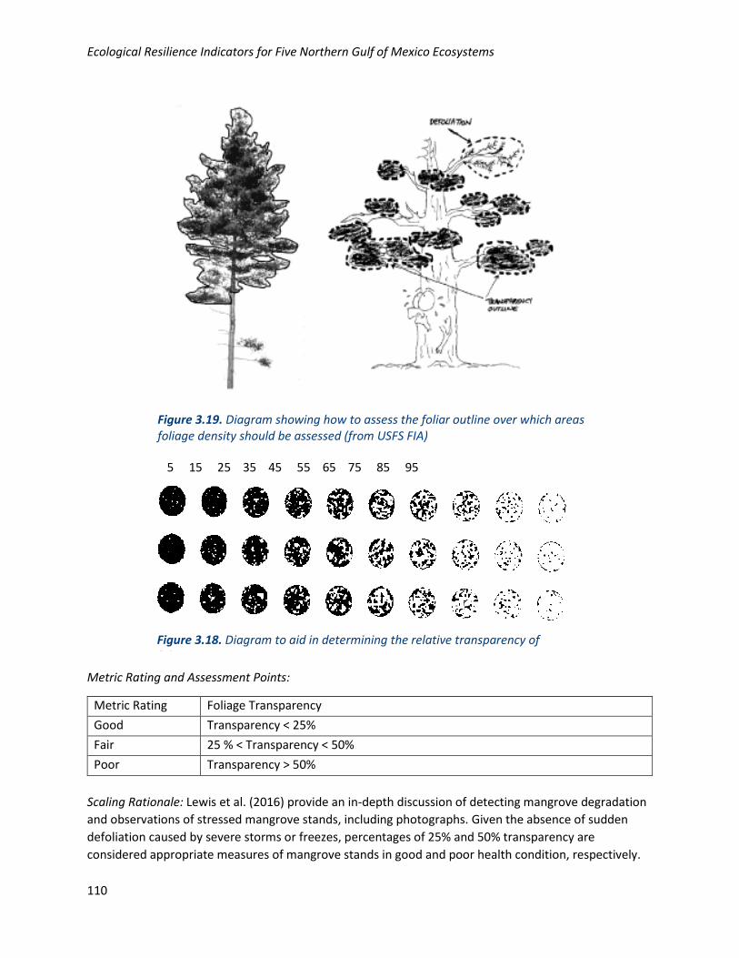
Measure: Measures were adapted from the US Forest Service Forest Inventory and Analysis (USFS FIA)
protocol, with adjustments necessary for mangrove forest structure; specifically, we assess the “foliage
transparency.” Only canopy trees (i.e., dominant/codominant) should be selected for analysis.
Tier: 2 (rapid field measurement)
Measurement: Foliage transparency is assessed by examining the crown of a tree, identifying where
branches support foliage, and then assessing the amount of light transmission through that foliage.
Figure 3.4 provides guidance on assessment of potential foliated outline, and Figure 3.5 on the relative
transmission through. Note that epicormic branches—shoots directly from dormant buds in a main
branch or stem—do not count as crown and thus receive a rating of 100% transparency. Likewise,
branches without foliage may still intercept light but should not be included in the rating (i.e., a fully
defoliated tree has a 100% transparency). Branches that are shaded and have apparently died because
of light competition and subsequent self-pruning (i.e., in deep shade) should not be treated as capable
of maintaining foliage. Foliage transparency should be assessed at 10 randomly selected points within
each monitoring plot. Due to differences between mangroves and other forests, we assess transparency
vertically and for a single field of view at 45 degrees from vertical.
Ecological Resilience Indicators for Five Northern Gulf of Mexico Ecosystems
110
Figure 3.19. Diagram showing how to assess the foliar outline over which areas foliage density should be assessed (from USFS FIA)
Metric Rating and Assessment Points:
Metric Rating Foliage Transparency
Good Transparency < 25%
Fair 25 % < Transparency < 50%
Poor Transparency > 50%
Scaling Rationale: Lewis et al. (2016) provide an in-depth discussion of detecting mangrove degradation
and observations of stressed mangrove stands, including photographs. Given the absence of sudden
defoliation caused by severe storms or freezes, percentages of 25% and 50% transparency are
considered appropriate measures of mangrove stands in good and poor health condition, respectively.
5 15 25 35 45 55 65 75 85 95
Figure 3.18. Diagram to aid in determining the relative transparency of foliage
Ecological Resilience Indicators for Five Northern Gulf of Mexico Ecosystems
111
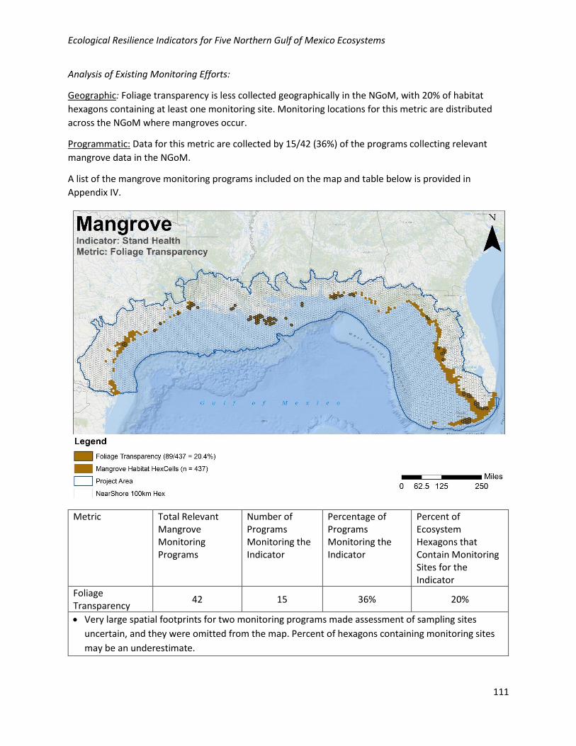
Analysis of Existing Monitoring Efforts:
Geographic: Foliage transparency is less collected geographically in the NGoM, with 20% of habitat
hexagons containing at least one monitoring site. Monitoring locations for this metric are distributed
across the NGoM where mangroves occur.
Programmatic: Data for this metric are collected by 15/42 (36%) of the programs collecting relevant
mangrove data in the NGoM.
A list of the mangrove monitoring programs included on the map and table below is provided in
Appendix IV.
Metric Total Relevant Mangrove Monitoring Programs
Number of Programs Monitoring the Indicator
Percentage of Programs Monitoring the Indicator
Percent of Ecosystem Hexagons that Contain Monitoring Sites for the Indicator
Foliage Transparency
42 15 36% 20%
• Very large spatial footprints for two monitoring programs made assessment of sampling sites
uncertain, and they were omitted from the map. Percent of hexagons containing monitoring sites
may be an underestimate.
Ecological Resilience Indicators for Five Northern Gulf of Mexico Ecosystems
112
Indicator: Regeneration Potential
MEF: Ecosystem Structure
KEA: Plant Community Structure
Metric: Propagule, Seedling, Sapling Presence
Definition: The density of mangrove species (R. mangle, A. germinans, L. racemosa) seedlings (< 1 m tall)
and saplings (< 2.5 cm diameter) (Baldwin et al., 2001) and seed propagules over a given area.
Background: The condition of a stand goes well beyond simply examining canopy structure because the
regeneration potential indicates the system’s long-term viability. In the absence of regeneration
potential, a disturbance event can trigger a direction state change away from the target system. Mature
trees generally better tolerate stress, which means that conditions that alter stand condition may be
seen more readily in saplings and seedlings.
Rational for Selection of Variable: All metrics are indicators of the ability for gaps to be filled, recover
from disturbance, and general suitability of mangroves for the present abiotic conditions.
Measure: Mean density of seedlings, saplings, and viable propagules across 10 plots
Tier: 3 (intensive field measurement)
Measurement: For a given assessment site, establish 10 randomly placed 5 × 5 m plots. Within each plot,
count number of seedlings, saplings, and viable propagules. Calculate mean of the 10 plots.
Metric Rating and Assessment Points:
Metric Rating Propagule, Seedling, Sapling Presence
Good > 1 seedling or sapling per plot
Fair < 1 seedling or sapling per plot and propagules are present
Poor < 1 seedling per plot and propagules are absent
Scaling Rationale: While more seedlings and saplings would be ideal, it is reasonable for them to be
absent under dense canopies because of light competition. However, if suitable establishment
conditions exist, there will always be some seedlings and/or saplings because of natural heterogeneities
in the light environment. Thus, the average over 10 plots is used. Presence of propagules is considered
sufficient to indicate the potential for a sustainable stand, so a fair rating is assigned.
Analysis of Existing Monitoring Efforts:
Geographic: Propagule, seedling, or sapling presence is less collected geographically in the NGoM, with
22% of habitat hexagons containing at least one monitoring site. Monitoring locations for this metric are
relatively well distributed across the NGoM where mangroves occur.
Programmatic: Data for this metric are collected by 13/42 (31%) of the programs collecting relevant
mangrove data in the NGoM.
A list of the mangrove monitoring programs included on the map and table below is provided in
Appendix IV.
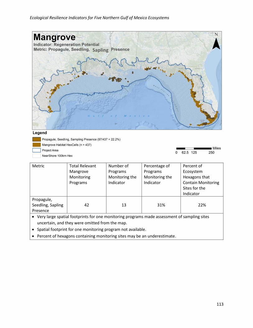
Ecological Resilience Indicators for Five Northern Gulf of Mexico Ecosystems
113
Metric Total Relevant Mangrove Monitoring Programs
Number of Programs Monitoring the Indicator
Percentage of Programs Monitoring the Indicator
Percent of Ecosystem Hexagons that Contain Monitoring Sites for the Indicator
Propagule, Seedling, Sapling Presence
42 13 31% 22%
• Very large spatial footprints for one monitoring programs made assessment of sampling sites
uncertain, and they were omitted from the map.
• Spatial footprint for one monitoring program not available.
• Percent of hexagons containing monitoring sites may be an underestimate.
Ecological Resilience Indicators for Five Northern Gulf of Mexico Ecosystems
114
Indicator: Land Aggregation
MEF: Ecosystem Structure
KEA: Landscape Structure
Metric: Aggregation Index (AI)
Definition: The physical structure of the landscape, accounting for topography, spatial distribution, and
shape of land and water elements. This structure can partially be described quantitatively by the
number of identical adjacent pixels of either water or land per pixel.
Background: The lateral erosion and vertical subsidence of coastal ecosystems are both related to the
shape of the landscape. Subsidence generally occurs in interior areas (Lewis et al., 2016), and thus the
land form can suggest the relative degradation (Couvillion et al., 2016). The organization of the
landscape structure is highly indicative of past changes and future trajectory (Kennish, 2001).
Rational for Selection of Variable: The organization of the landscape differs between healthy and
degraded mangrove forest, with a degraded or degrading system showing evidence of increased
erosion, increased open water, and increased fragmentation of the landscape. In addition to indicating
loss, AI is important to quality of habitat.
Measure: Landsat 30 m pixels classified as water, unvegetated mudflats, marsh, or mangrove
Tier: 1 (remotely sensed)
Measurement: Remote sensing (tier 1) techniques with Landsat data (30 m resolution) will provide the
data needed to calculate AI, a metric quantifying the fraction of pixels with adjacent pixels of the same
classification. Winter images should be used because of the distinction between senescent marsh and
evergreen mangroves during the winter. Precise methodological details are in Couvillion et al. (2016).
This requires classifying the pixel as either water, marsh, or mangrove, and then applying the analysis
directly to the raster of classified pixels. AI was calculated for a given area of interest (AOI):
𝐴𝐼 = ∑𝐴𝑑𝑗𝑎𝑐𝑒𝑛𝑐𝑖𝑒𝑠 𝑝𝑒𝑟 𝑝𝑖𝑥𝑒𝑙
𝐶𝑙𝑎𝑠𝑠 𝑃𝑖𝑥𝑒𝑙 𝐶𝑜𝑢𝑛𝑡 × 8 × 𝑃𝑒𝑟𝑐𝑒𝑛𝑡 𝐴𝑂𝐼
yielding values from zero to 100, with Adjacencies Per Pixel = the number of adjacencies of like class
value per pixel, Class Pixel Count = the number of pixels of the class within the AOI, and Percent AOI =
the percent area occupied by the class within the AOI. The aggregation index should be calculated as a
moving average across 250 m square AOIs for a landscape level assessment (integrating mangrove,
marsh, and open water; Couvillion et al. 2016).
Metric Ratings and Assessment Points:
Metric Rating Aggregation Index (AI)
Good Aggregation Index is > 80%
Fair Aggregation Index is 50–80%
Poor Aggregation Index is < 50%
Ecological Resilience Indicators for Five Northern Gulf of Mexico Ecosystems
115
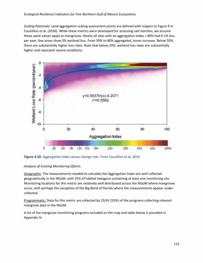
Scaling Rationale: Land aggregation scaling assessment points are defined with respect to Figure 9 in
Couvillion et al. (2016). While these metrics were developed for assessing salt marshes, we assume
these same values apply to mangroves. Nearly all sites with an aggregation index > 80% had 0-1% loss
per year; few areas show 0% wetland loss. From 50% to 80% aggregated, losses increase. Below 50%,
there are substantially higher loss rates. Note that below 20%, wetland loss rates are substantially
higher and represent severe conditions.
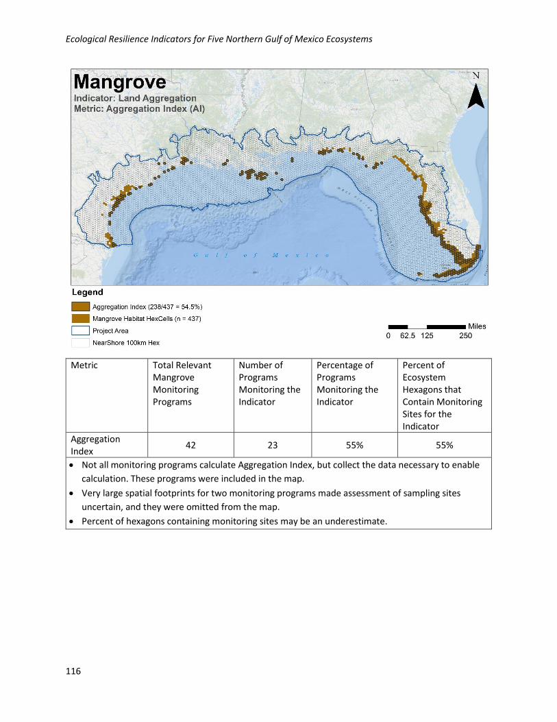
Analysis of Existing Monitoring Efforts:
Geographic: The measurements needed to calculate the Aggregation Index are well collected
geographically in the NGoM, with 55% of habitat hexagons containing at least one monitoring site.
Monitoring locations for this metric are relatively well distributed across the NGoM where mangroves
occur, with perhaps the exception of the Big Bend of Florida where the measurements appear under-
collected.
Programmatic: Data for this metric are collected by 23/42 (55%) of the programs collecting relevant
mangrove data in the NGoM.
A list of the mangrove monitoring programs included on the map and table below is provided in
Appendix IV.
Figure 4.20. Aggregation index versus change rate. From Couvillion et al, 2016.
Ecological Resilience Indicators for Five Northern Gulf of Mexico Ecosystems
116
Metric Total Relevant Mangrove Monitoring Programs
Number of Programs Monitoring the Indicator
Percentage of Programs Monitoring the Indicator
Percent of Ecosystem Hexagons that Contain Monitoring Sites for the Indicator
Aggregation Index
42 23 55% 55%
• Not all monitoring programs calculate Aggregation Index, but collect the data necessary to enable
calculation. These programs were included in the map.
• Very large spatial footprints for two monitoring programs made assessment of sampling sites
uncertain, and they were omitted from the map.
• Percent of hexagons containing monitoring sites may be an underestimate.
Ecological Resilience Indicators for Five Northern Gulf of Mexico Ecosystems
117
Indicator: Land Cover Change
MEF: Ecosystem Structure
KEA: Landscape Structure
Metric: Land Cover Change Rate
Definition: Rate of expansion or contraction of vegetative cover over a five-year period.
Background: Mangrove areal coverage within a landscape may contract or expand due to a variety of
factors. Contraction is cause by lateral erosion, dieback within stagnated basin stands, or freeze dieback
at the northern fringe of each mangrove species’ distribution in the NGoM. Expansion may occur onto
newly formed mudflats after deposition events, ingrowth into basin mangrove stands after hydrology is
restored, or poleward expansion during warm years lacking freeze mortality events (Diop et al., 1997;
Eslami-Andargoli et al., 2009).
Rational for Selection of Variable: Physical loss of mangroves due to dieback or erosion is unhealthy for
ecosystem sustainability. Likewise, expansion of mangrove habitat indicates conditions favorable for
growth.
Measure: Landsat 30 m pixels classified as mangrove in a series of images spanning a five-year period
Tier: 1 (remotely sensed)
Measurement: Remote sensing (tier 1) techniques with Landsat data (30 m resolution) will provide the
data needed to calculate the areal extent of mangroves in the landscape. Winter images should be used
because of the distinction between senescent marsh and evergreen mangroves during the winter. Pixels
covering a chosen area are classified as mangrove or non-mangrove in least one image per year for five
years. The rate of change is calculated from the difference in mangrove pixel count between years
divided by the number of years.
Metric Rating and Assessment Points:
Metric Rating Land Cover Change Rate
Excellent Mangrove areal cover expands at a rate detectable by remote sensing
Good Mangrove areal cover stable
Fair Mangrove areal cover contracts at a slow rate (< 10%) detectable by remote sensing
Poor Mangrove areal cover contracts at a rapid rate (> 10%) detectable by remote sensing
Scaling Rationale: Mangrove expansion indicates conditions favorable to growth, while mangrove
contraction indicates a condition (acute or chronic) causing loss of vegetative cover.
Analysis of Existing Monitoring Efforts:
Geographic: Land cover change rate is well collected geographically in the NGoM, with 54% of habitat
hexagons containing at least one monitoring site. Monitoring locations for this metric are relatively well
distributed across the NGoM where mangroves occur, with perhaps the exception of the Big Bend area
of Florida, where the metric seems under-collected.
Ecological Resilience Indicators for Five Northern Gulf of Mexico Ecosystems
118
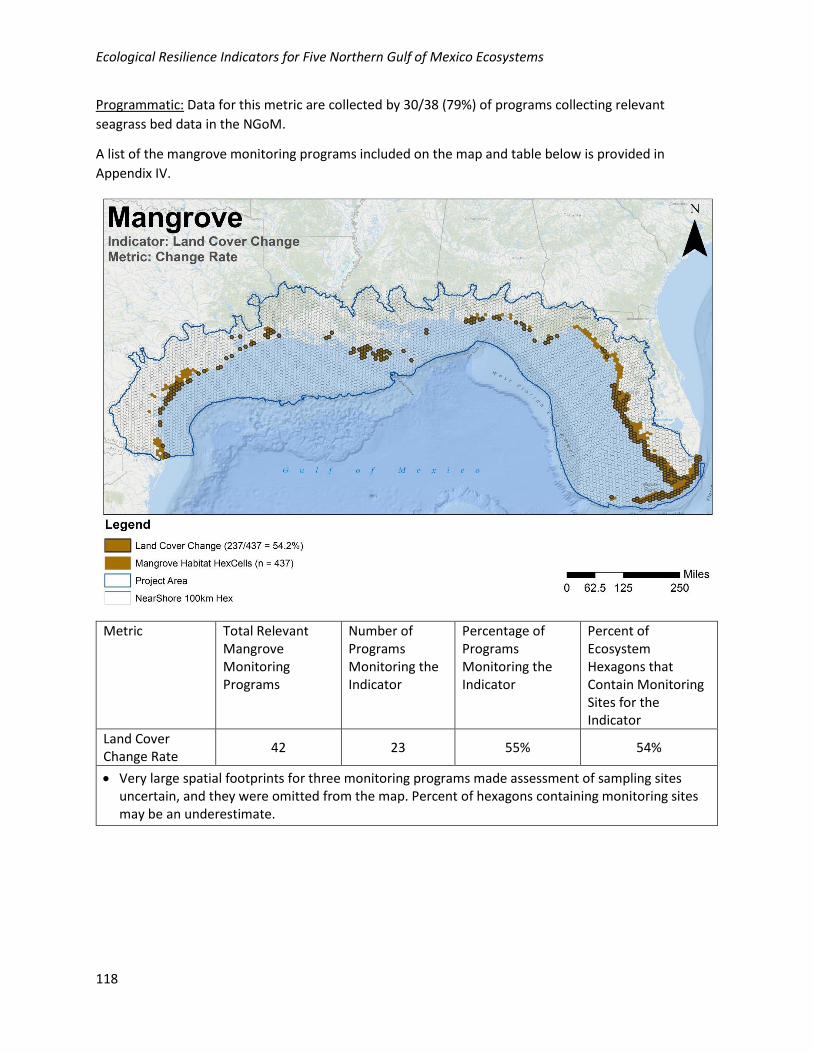
Programmatic: Data for this metric are collected by 30/38 (79%) of programs collecting relevant
seagrass bed data in the NGoM.
A list of the mangrove monitoring programs included on the map and table below is provided in
Appendix IV.
Metric Total Relevant Mangrove Monitoring Programs
Number of Programs Monitoring the Indicator
Percentage of Programs Monitoring the Indicator
Percent of Ecosystem Hexagons that Contain Monitoring Sites for the Indicator
Land Cover Change Rate
42 23 55% 54%
• Very large spatial footprints for three monitoring programs made assessment of sampling sites uncertain, and they were omitted from the map. Percent of hexagons containing monitoring sites may be an underestimate.
Ecological Resilience Indicators for Five Northern Gulf of Mexico Ecosystems
119
Indicator: Submergence Vulnerability
MEF: Ecosystem Function
KEA: Elevation Change
Metric: Wetland Relative Sea Level Rise (RSLRwet) and Submergence Vulnerability Index (SVI)
Definition: The rate of change in marsh surface elevation with respect to a hydrologic datum.
Background: Mangrove elevation increases with organic and mineral accretion, largely related to root
growth (McKee, 2011; McKee et al., 2007). Elevation change can be used as a measure of resilience to
sea-level rise. Low tidal ranges result in greater vulnerability because of lower accretion rates (Cahoon
et al., 2006). Due to the importance of root growth, any alteration to root-to-shoot ratios or overall
reduction in production could limit ability to maintain elevation.
Rational for Selection of Variable: Elevation change indicates vulnerability to submergence when
compared with sea-level rise (Cahoon, 2015). Wetland elevation should be measured alongside water
level to quantify wetland relative sea-level rise (RSLRwet), which is the difference between tide gauge
RSLR and wetland surface elevation (Cahoon et al., 2015). An elevation rate deficit (sea level rising
compared to wetland elevation) indicates vulnerability, whereas an elevation rate surplus (sea level
falling compared to wetland elevation) indicates stability. However, because RSLRwet only considers
differences between the water and wetland trajectories, this would mischaracterize the vulnerability of
a wetland that is situated high in the tidal frame that will likely change types (depending on climate) as
sea level rises (e.g., Osland et al., 2014). Therefore, when possible, an index of relative elevation within
the tidal frame must also be used (submergence vulnerability index, SVI; Stagg et al., 2013) in
complement to RSLRwet.
Measure: The rate of change in wetland surface elevation, based on rod surface elevation tables (RSET)
with respect to a hydrologic datum
Tier: 3 (intensive field measurement)
Measurement: Elevation change is measured using rod surface elevation tables (RSET; Cahoon et al.,
2002a, 2002b). The elevation of the wetland surface relative to a fixed datum, established by a rod
driven into the substrate until refusal, is measured periodically. Surface elevation change is quantified
by estimating the change in wetland surface elevation over time using linear regression. Surface
elevation change represents surface and subsurface processes occurring between the wetland surface
and the bottom of the rod benchmark (Cahoon et al., 2002a). RSET locations are currently installed in
many locations across NGoM states. SETs are generally measured at six-month intervals, with data
quality improving over length of measurement. Further details are available at
http://www.pwrc.usgs.gov/set/. SET measurements should be paired with water level measurements
and sea level rise rates. NGoM sea level rise rates ranges from 1.38 mm yr-1 to 9.65 mm yr-1, with highest
values from Mississippi through east Texas, and with lower values on the Florida and Alabama coasts
(Pendleton et al., 2010).
The calculation of SVI is a comparison of projected elevation to projected tidal range to assess not only
the differences in trajectories, but also the relative position of the wetland within that tidal range. The
SVI is a projection of wetland flooding frequency five years into future, accounting for tidal amplitude,
periodicity, and projected site relative elevation. In addition to long-term RSET and hydrologic data,
Ecological Resilience Indicators for Five Northern Gulf of Mexico Ecosystems
120
wetland and water elevation must be referenced to a common datum (NAVD 88) to calculate the SVI
(Stagg et al., 2013).
Metric Rating and Assessment Points:
Metric Rating RSLRwet and SVI
Good RSLRwet is negative or stationary (sea level falling relative to wetland), or RSLRwet is positive and SVI > 50
Poor RSLRwet is positive (sea level rising relative to wetland) and SVI < 50
Scaling Rationale: Good conditions are met when the wetland elevation is either matching or exceeding
sea level rise. Poor conditions occur when the wetland elevation is declining relative to sea level, which
indicates that wetland is submerging. When RSLRwet is positive but the salt wetland elevation is high (SVI
> 50), the wetland cannot be considered unstable. Although wetlands situated higher in the tidal frame
may have a negative elevation trajectory, due to low rates of production associated with little flooding,
the wetland is not excessively flooded or at risk of submergence.
Analysis of Existing Monitoring Efforts:
Geographic: Wetland relative sea level rise (RSLRwet) and submergence vulnerability index (SVI) are well
collected geographically in the NGoM, with 52% of habitat hexagons containing at least one monitoring
site. Monitoring locations for this metric are relatively well distributed across the NGoM where
mangroves occur.
Programmatic: Data for this metric are collected by 19/42 (45%) of the programs collecting relevant
mangrove data in the NGoM.
A list of the mangrove monitoring programs included on the map and table below is provided in
Appendix IV.
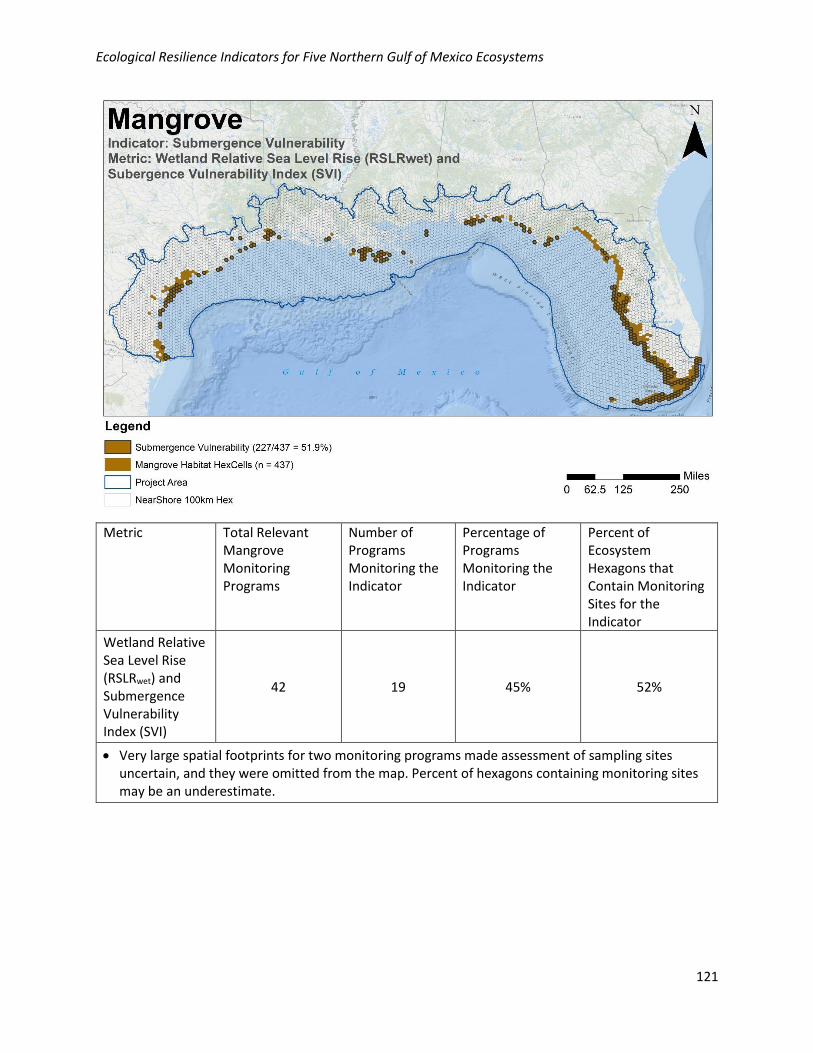
Ecological Resilience Indicators for Five Northern Gulf of Mexico Ecosystems
121
Metric Total Relevant Mangrove Monitoring Programs
Number of Programs Monitoring the Indicator
Percentage of Programs Monitoring the Indicator
Percent of Ecosystem Hexagons that Contain Monitoring Sites for the Indicator
Wetland Relative Sea Level Rise (RSLRwet) and Submergence Vulnerability Index (SVI)
42 19 45% 52%
• Very large spatial footprints for two monitoring programs made assessment of sampling sites uncertain, and they were omitted from the map. Percent of hexagons containing monitoring sites may be an underestimate.
Ecological Resilience Indicators for Five Northern Gulf of Mexico Ecosystems
122
Indicator: Fish Habitat
MEF: Ecosystem Function
KEA: Secondary Production
Metric: Killifish Species Diversity
Definition: Fish habitat is assessed by diversity of killifish, which includes any egg-laying
cyprinodontiform fish, spanning across several families.
Background: Killifish are generally small (1–2 inches) and feed on insects, crustaceans, algae, or worms.
As abundant small fish, they constitute an important energy source to high trophic level organisms.
Rational for Selection of Variable: Given their importance to higher trophic levels and their advantage
associated with mangrove forest structure (Laegdsgaard and Johnson, 2001), presence of killifish
indicates system health. Diversity specifically is assessed because while some species are common
generalists and widespread (e.g., mosquitofish), others (e.g., mangrove rivulus) are mangrove specialists
(Davis et al., 1995).
Measure: Number of killifish species
Tier: 3 (intensive field measurement)
Measurement: Standard fish collection methods may be used which are suitable for mangrove habitats
such as throw traps, pull traps, drop nets, or minnow traps (Trexler et al., 2000), and adapted to
maximize the catch of small fish.
Metric Rating and Assessment Points:
Metric Rating Killifish Species Diversity
Good More than one killifish species present
Fair One killifish species present
Poor No killifish present
Scaling Rationale: Presence of more than one killifish species indicates mangrove ecosystem conditions
are diverse enough to include killifish species with differing requirements. Presence of only one killifish
species may indicate a condition very specific for the survival of that species although deleterious to
other species. No killifish present in a mangrove stand is indicative of a system that has a poor food web
structure, since killifish are near the base of the secondary producer food chain and are fed upon by fish
as well as wading birds (Day et al., 1989).
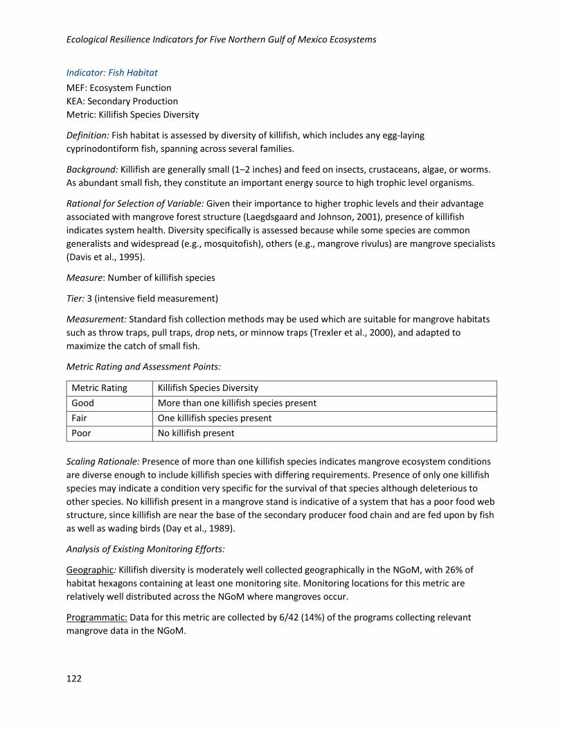
Analysis of Existing Monitoring Efforts:
Geographic: Killifish diversity is moderately well collected geographically in the NGoM, with 26% of
habitat hexagons containing at least one monitoring site. Monitoring locations for this metric are
relatively well distributed across the NGoM where mangroves occur.
Programmatic: Data for this metric are collected by 6/42 (14%) of the programs collecting relevant
mangrove data in the NGoM.
Ecological Resilience Indicators for Five Northern Gulf of Mexico Ecosystems
123
A list of the mangrove monitoring programs included on the map and table below is provided in
Appendix IV.
Metric Total Relevant Mangrove Monitoring Programs
Number of Programs Monitoring the Indicator
Percentage of Programs Monitoring the Indicator
Percent of Ecosystem Hexagons that Contain Monitoring Sites for the Indicator
Killifish Diversity 42 6 14% 26%
• Very large spatial footprints for one monitoring programs made assessment of sampling sites uncertain, and they were omitted from the map. Percent of hexagons containing monitoring sites may be an underestimate.
Ecological Resilience Indicators for Five Northern Gulf of Mexico Ecosystems
124
Indicator: Invasive Species
MEF: Ecosystem Function
KEA: Secondary Production
Metric: Presence (Multiple Species)
Definition: Presence of invasive species that have a detrimental effect on the ecosystem function,
including: Nilgai (Boselaphus tragocamelus), lionfish (Pterois miles and Pterois volitans), feral pig (Sus
scrofa), and python (Python bivittatus).
Background: Various invasive species have become common within the mangrove ecosystems, but with
varying detrimental effects. Nilgai (an antelope introduced from India to Texas hunting ranches) and
feral pigs are large mammals which directly disturb vegetation through trampling and/or feeding on
vegetation (Leslie, 2016). The Rhizophora borer (Coccotrypes rhizophorae) can destroy propagules and
also directly invade trees. The lionfish and pythons are both invasive predators that can substantially
alter the trophic dynamics (Barbour et al., 2010). Other species may be present (e.g., iguana, monitor
lizard, cichlids), although they are less likely to have large systemic impacts. Others have substantial
impacts but are not easily detectable and thus are not useful as an indicator (e.g., Rhizophora borer).
Two species of non-native mangroves were introduced into south Florida (Bruguiera gymnorrhiza and
Lumnitzera racemosa), which were competing directly for space with native mangroves (Fourqurean et
al., 2010). Efforts to eradicate mature individuals of these invasive mangroves have been successful thus
far, but saplings continue to reappear, possibly posing a threat in the future if control is relaxed.
Rational for Selection of Variable: The presence of these species necessarily involves an alteration to the
ecosystem function at the specific site observed, constituting an important variable to measure.
Measures/Measurement:
Nilgai evidence: Nilgai leave widespread evidence of browsing and tracks (detectable by aerial image).
Currently, this is only relevant to Texas ecosystems.
Feral pig evidence: Similarly, feral pig presence can be identified by the presence of tracks, root foraging,
or wallows.
Lionfish evidence: Use of citizen science observations presents an effective solution for monitoring
lionfish presence (Scyphers et al., 2014). In sites that have tourism, recreation, and fishery uses,
establishing a system for reporting observations can identify where lionfish are.
Python evidence: Currently pythons are only known to exist in south Florida ecosystems where
extensive detection, monitoring, and eradication programs are already in progress, using multiple
methods (e.g., eDNA and dogs; Avery, 2014; Hunter, 2015). While they are elusive, monitoring agencies
should contact local wildlife management agencies for further information.
Tier: 2 (rapid field measurement)
Ecological Resilience Indicators for Five Northern Gulf of Mexico Ecosystems
125
Metric Rating and Assessment Points:
Metric Rating Presence (Multiple Species)
Good No evidence of invasive species
Fair Evidence of invasive species, but not affecting vegetation structure
Poor Evidence of invasive species altering vegetation structure
Scaling Rationale: If invasive species alter the vegetation structure, this receives a poor rating because
structural alterations affect related functions (e.g., elevation maintenance, habitat, production,
regeneration potential) and many ecological services (e.g., aesthetics, habitat values). In contrast,
invasives that do not directly affect structure (e.g., lionfish) will likely only directly affect the secondary
producers and not affect other important functions.
Analysis of Existing Monitoring Efforts:
Geographic: Invasive species presence is well collected geographically in the NGoM, with 52% of habitat
hexagons containing at least one monitoring site. Monitoring locations for this metric are relatively well
distributed across the NGoM where mangroves occur, with lower collection rates in the Big Bend area of
Florida.
Programmatic: Data for this metric are collected by 15/42 (36%) of the programs collecting relevant
mangrove data in the NGoM.
A list of the mangrove monitoring programs included on the map and table below is provided in
Appendix IV.
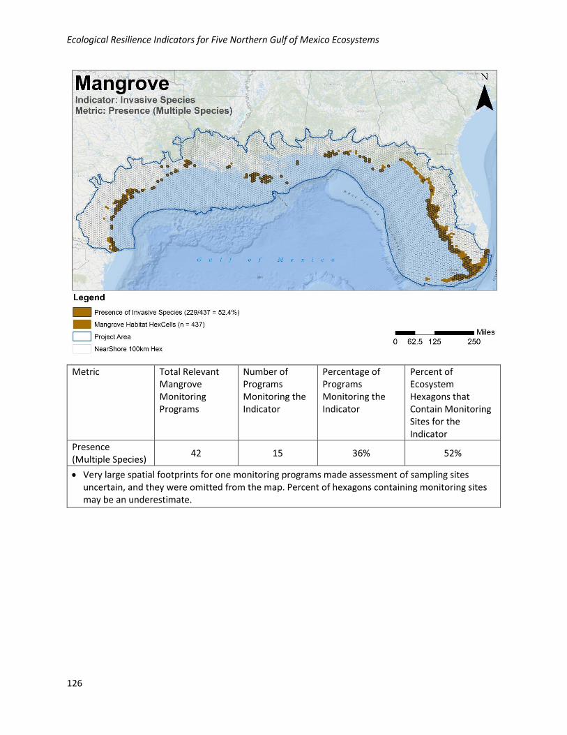
Ecological Resilience Indicators for Five Northern Gulf of Mexico Ecosystems
126
Metric Total Relevant Mangrove Monitoring Programs
Number of Programs Monitoring the Indicator
Percentage of Programs Monitoring the Indicator
Percent of Ecosystem Hexagons that Contain Monitoring Sites for the Indicator
Presence (Multiple Species)
42 15 36% 52%
• Very large spatial footprints for one monitoring programs made assessment of sampling sites uncertain, and they were omitted from the map. Percent of hexagons containing monitoring sites may be an underestimate.
Ecological Resilience Indicators for Five Northern Gulf of Mexico Ecosystems
127
Ecosystem Service Indicators
Indicator: Status of Macrofauna Population
MES: Supporting and Provisioning
KES: Habitat
Metric: Density of Juvenile Common Snook
Definition: Number of individuals of juvenile (standard length [SL] <= 25.4 cm [10 in]) common snook
(Centropomus undecimalis), per unit area.
Background: Snook are subtropical euryhaline fishes with a strong preference for mangrove estuarine
habitats. Of the five species that occur in Florida, common snook (Centropomus undecimalis) is the most
common and popular inshore game fish in Florida (other snook species:
http://myfwc.com/research/saltwater/fish/snook/sketch-common-snook/). Juvenile snook are found
between freshwater rivers to mangrove-fringed estuarine coast until they reach about 10 to 14 inches
long. After this they reach sexual maturity and move to higher-salinity areas of the estuaries. Their
habitat preference lies in the common characteristics of mangrove forest habitat of good water quality,
moderate slope in banks, slow currents, overhanging vegetation that provides shade, and the structure
that is provided by the mangrove root system (Seaman and Collins, 1983).
Rationale for Selection of Variable: The fish densities used were estimated by Brame (2012) in the study
of juvenile common snook along mangrove shoreline in Frog Creek, a tidal tributary of Tampa Bay,
Florida. Density constitutes an important statistic to describe and understand wild populations. It allows
for the assessment of population resource utilization at a specific habitat. The measurement of density
is relevant when dealing with resident small fish and invertebrates when the goal is to assess complex
areas (Beck et al., 2001) and where visual census is not suitable.
Measure: Individuals per square meter. Field-collected organisms should be identified and enumerated.
Tier: 3 (intensive field measurement)
Measurement: Standard fish collection methods may be used which are suitable for mangrove habitats
such as throw traps, pull traps, drop nets, or minnow traps (Trexler et al., 2000). Record all organisms,
and data should be presented on individuals/m2. Conduct field measures at different areas of the
estuaries such as upstream and downstream where the salinity gradient is different.
Metric Rating and Assessment Points:
Metric Rating Density of Juvenile* Common Snook (Centropomus undecimalis)
Upstream (ponds and creeks mean) Downstream (ponds and creeks mean)
Good–Excellent >= 7.0 fish/100m2 or stable/increasing >= 2.6 fish/100m2 or stable/increasing
Poor < 7.0 fish/100m2 or decreasing < 2.6 fish/100m2 or decreasing
*Ratings here are provided for young of the year fish < 150 mm SL.
Scaling Rationale: The fish densities used were estimated by Brame (2012) in the study of juvenile
common snook along mangrove shoreline in Frog Creek, a tidal tributary of Tampa Bay, Florida. Density
values above the published mean from Brame (2012) are considered good to excellent population
health. Fish densities below are considered poor. Densities at different salinity gradients—i.e., upstream
Ecological Resilience Indicators for Five Northern Gulf of Mexico Ecosystems
128
and downstream estuarine areas—are presented. Since the available assessment points are available
from only one study, if densities vary significantly from the suggested values, employ the
stable/increasing/decreasing metric ratings instead.
Analysis of Existing Monitoring Efforts:
No programs in the monitoring program inventory specifically noted collection of data on snook
densities.
Ecological Resilience Indicators for Five Northern Gulf of Mexico Ecosystems
129
Indicator: Status of Snapper-Grouper Complex Commercial Fishery
MES: Provisioning
KES: Food
Metric 1: Gray Snapper Density
Metric 2: Commercial Landings of Gray Snapper
Metric 1: Gray Snapper Density
Definition: Number of individuals of gray snapper per unit area.
Background: Gray snapper (also known as gray mangrove snapper or mangrove snapper) is a shallow
species common to mangroves. Adults seek shelter in warm temperate reefs, mangroves, and seagrass
habitats throughout the entire Gulf of Mexico. Juveniles typically settle in suitable estuarine habitat such
as mangroves. Spatial and temporal dynamic analysis of their diel migratory movements using acoustic
tagging and video show that shallow seagrass beds are frequented nocturnally and mangroves are
occupied diurnally (Luo et al., 2009).
Gray snapper constitutes an important commercial fishery species that has been monitored nearly
continuously since 1958 in Florida and along the southeast U.S. coast (Rutherford et al., 1989). The
species is sought largely as a seasonal supplement to other fisheries. Gray snapper fisheries are
managed by federal and state agencies using common regulations, and commercial and recreational
annual catch limits are set every year in the NGoM. Although its abundance on the Atlantic and Gulf
coasts is unknown, it appears to have remained mostly stable over the last few decades. However, in the
south Florida region, it is likely that gray snapper is overfished (Burton, 2001;
http://safinacenter.org/documents/2014/08/mangrove-snapper-u-s-full-species-report.pdf). In the
NGoM, a combined commercial and recreational annual catch limit (ACL) has been set at 1,097 metric
tons (GMFMC, 2011).
Rationale for Selection of Variable: Density allows for the assessment of population resource utilization
at a specific site and provides an indication of the potential for a site to contribute to commercial
fishing. It is not a direct measure of the ecosystem service because little is known about population
dynamics and fisheries impacts. This metric is best used when it is important to tie the ecosystem
service to a specific site.
Measure: Number individuals m-2
Tier: 3 (intensive field measurement)
Measurement: Standard fish collection methods may be used which are suitable for mangrove habitats
such as throw traps, pull traps, drop nets, and/or minnow traps (Trexler et al., 2000). Record all
organisms, and data should be presented on individuals/m2. Field-collected organisms should be
identified and enumerated by age/size class. Conduct annual field measurements.
Metric Rating and Assessment Points:
Metric Rating Density of Gray Snapper (or significant change in age/size class distribution)
Good Increasing/stable
Poor Decreasing
Ecological Resilience Indicators for Five Northern Gulf of Mexico Ecosystems
130
Scaling Rationale: Specific expected densities at given sites are not available to establish assessment
points. Decreases in gray snapper density would indicate a decrease in a site’s capacity to provide fish
for commercial fisheries. Changes in age/size class distribution (e.g., a decline in juveniles over time)
may also indicate potential for declining contribution to recreational fisheries.
Analysis of Existing Monitoring Efforts:
No programs in the monitoring program inventory specifically noted collection of gray snapper data.
Data for this resource is gathered by the Marine Recreational Information Program (MRIP) and can be
accessed at: https://www.st.nmfs.noaa.gov/recreational-fisheries/data-and-
documentation/queries/index. No map or hexagon distribution statistics were calculated.
Metric 2: Commercial Landings of Gray Snapper
Definition: Annual commercially landed weight of gray snapper (Lutjanus griseus).
Background: Gray snapper (also known as gray mangrove snapper or mangrove snapper) is a shallow
species common to mangroves. Adults seek shelter in warm temperate reefs, mangroves, and seagrass
habitats throughout the entire Gulf of Mexico. Juveniles typically settle in suitable estuarine habitat such
as mangroves. Spatial and temporal dynamic analysis of their diel migratory movements using acoustic
tagging and video show that shallow seagrass beds are frequented nocturnally and mangroves are
occupied diurnally (Luo et al., 2009).
Gray snapper constitutes an important commercial fishery species that has been monitored nearly
continuously since 1958 in Florida and along the southeast U.S. coast (Rutherford et al., 1989). The
species is sought largely as a seasonal supplement to other fisheries. Gray snapper fisheries are
managed by federal and state agencies using common regulations, and commercial and recreational
annual catch limits are set every year in the NGoM. Although its abundance on the Atlantic and Gulf
coasts is unknown, it appears to have remained mostly stable over the last few decades. However, in the
south Florida region, it is likely that gray snapper is overfished (Burton, 2001;
http://safinacenter.org/documents/2014/08/mangrove-snapper-u-s-full-species-report.pdf). In the
NGoM, a combined commercial and recreational annual catch limit (ACL) has been set at 1,097 metric
tons (GMFMC, 2011).
Rationale for Selection of Variable: Commercial fishery landing statistics provide direct measure of the
degree of service enjoyed by humans. At best, current statistics are available annually at the state level
(but only for some states) and cannot assess the contribution of a given site to the ecosystem service.
This metric is best used to assess the potential contribution of mangroves to commercial fisheries at the
state or regional level on an annual basis. Note that this is somewhat confounded by the fact that gray
snapper use other estuarine habitats as well (such as seagrass and coral reefs).
Measure: Metric tons (t) of gray snapper landed per year
Tier: 3 (intensive field measurement)
Measurement: Assess the total weight of gray snapper annually using recreational fishery statistics
reported by the National Marine Fishery Service (NMFS). Federal and state data are available at the
Annual Commercial Landings Statistics site of the NMFS at
http://www.st.nmfs.noaa.gov/st1/commercial/landings/annual_landings.html. Statistics for each state
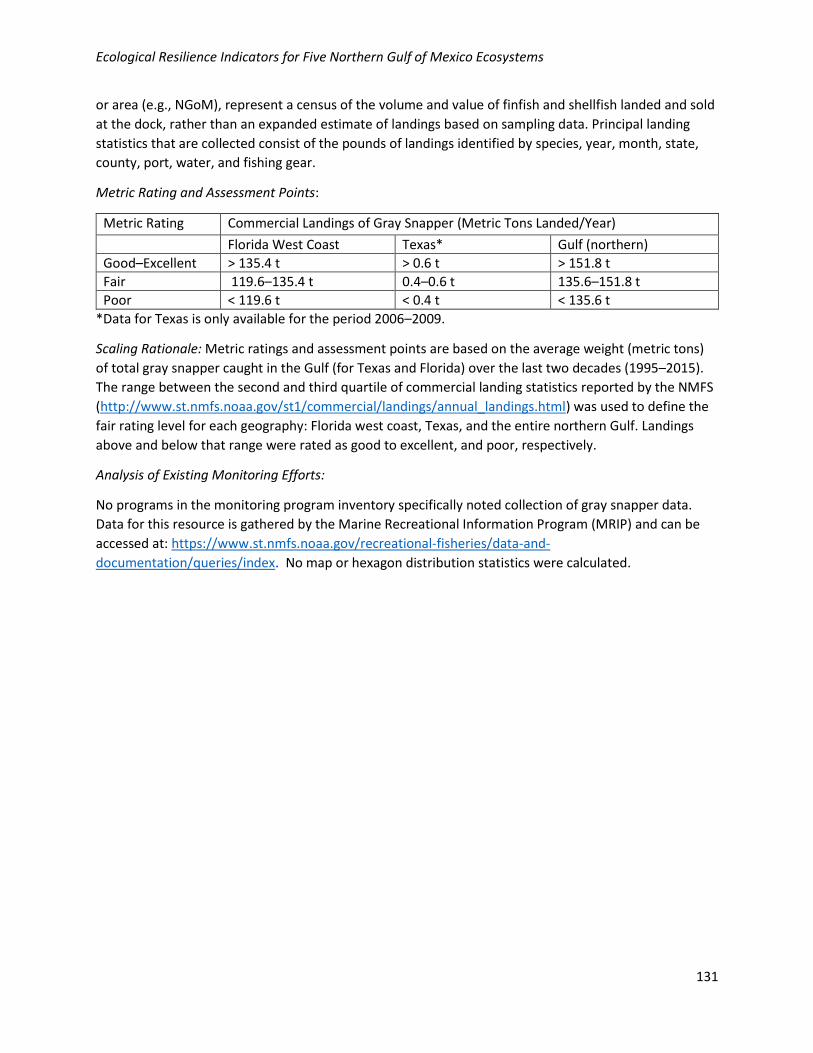
Ecological Resilience Indicators for Five Northern Gulf of Mexico Ecosystems
131
or area (e.g., NGoM), represent a census of the volume and value of finfish and shellfish landed and sold
at the dock, rather than an expanded estimate of landings based on sampling data. Principal landing
statistics that are collected consist of the pounds of landings identified by species, year, month, state,
county, port, water, and fishing gear.
Metric Rating and Assessment Points:
Metric Rating Commercial Landings of Gray Snapper (Metric Tons Landed/Year)
Florida West Coast Texas* Gulf (northern)
Good–Excellent > 135.4 t > 0.6 t > 151.8 t
Fair 119.6–135.4 t 0.4–0.6 t 135.6–151.8 t
Poor < 119.6 t < 0.4 t < 135.6 t
*Data for Texas is only available for the period 2006–2009.
Scaling Rationale: Metric ratings and assessment points are based on the average weight (metric tons)
of total gray snapper caught in the Gulf (for Texas and Florida) over the last two decades (1995–2015).
The range between the second and third quartile of commercial landing statistics reported by the NMFS
(http://www.st.nmfs.noaa.gov/st1/commercial/landings/annual_landings.html) was used to define the
fair rating level for each geography: Florida west coast, Texas, and the entire northern Gulf. Landings
above and below that range were rated as good to excellent, and poor, respectively.
Analysis of Existing Monitoring Efforts:
No programs in the monitoring program inventory specifically noted collection of gray snapper data.
Data for this resource is gathered by the Marine Recreational Information Program (MRIP) and can be
accessed at: https://www.st.nmfs.noaa.gov/recreational-fisheries/data-and-
documentation/queries/index. No map or hexagon distribution statistics were calculated.

Ecological Resilience Indicators for Five Northern Gulf of Mexico Ecosystems
132
Indicator: Erosion Reduction
MES: Regulating
KES: Coastal Protection
Metric: Shoreline Change
Definition: The statistically significant gain or loss in shoreline positions over a length of time.
Background: Shoreline protection capacity is provided by the relative inflexible plants that dissipate the
incoming wave energy due to their height and width, and dense structure along the shoreline (Betts,
2006; Marois and Mitsch, 2015). Suzuki et al. (2012) also provide various examples of wave attenuation
by mangroves.
Rationale for Selection of Variable: Shoreline stabilization constitutes an important measure of the risk
reduction benefits provided by mangroves. Mangrove vegetation absorbs wave energy that otherwise
would put at risk people, property, or landscapes (The Nature Conservancy, 2017).
Measure: Mangrove shoreline change in meters per year across permanent transects, and length of
affected shoreline
Tier: 1 (remotely sensed and modeled)
Measurement: To measure mangrove shoreline width, remote sensed data from the Landsat dataset can
be used if there is sufficient imagery within the appropriate time period (< 1 year from assessment date,
or after most recent major storm event, whichever is more recent). Repeat over a time period of
interest, such as a number of years in the past up to the present, or before and after storm.
Tier: 3 (intensive field measurement)
Measurement: Field measurements should be performed on the shoreline of the area adjacent to the
mangrove, and at a control site with similar current and wave conditions in the region. Repeat over a
time period of interest, such as a number of years in the past up to the present, or before and after a
storm. For a complete description of the methods, see The Nature Conservancy (2017).
Metric Rating and Assessment Points:
Metric Rating Shoreline Change (meters per/year and length of affected shoreline)
Good–Excellent No change, gain (accretion)
Poor Loss (erosion)
Scaling Rationale: Assessment points for indicator values constitute no change or positive (accretion)
and negative (erosion) changes in shoreline areas adjacent to the mangrove.
Analysis of Existing Monitoring Efforts:
Geographic: Shoreline change is moderately well collected geographically in the NGoM, with 27% of
habitat hexagons containing at least one monitoring site. Monitoring locations for this metric are mostly
collected in Florida, with a few monitoring sites in Texas.
Programmatic: Data for this metric are collected by 2/42 (5%) of the programs collecting relevant
mangrove data in the NGoM.
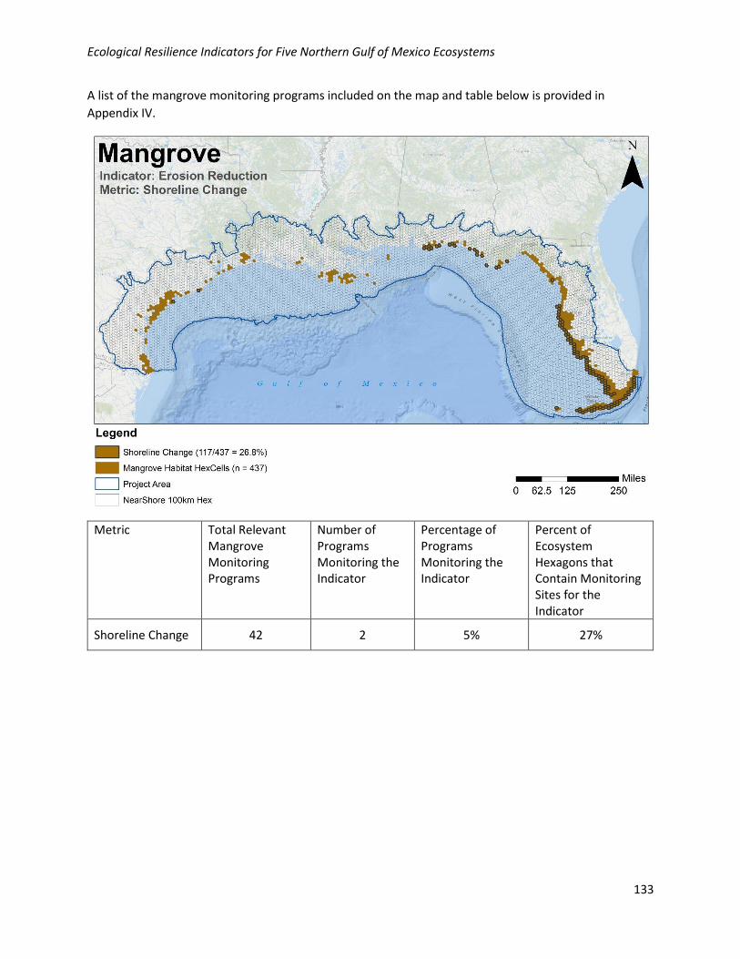
Ecological Resilience Indicators for Five Northern Gulf of Mexico Ecosystems
133
A list of the mangrove monitoring programs included on the map and table below is provided in
Appendix IV.
Metric Total Relevant Mangrove Monitoring Programs
Number of Programs Monitoring the Indicator
Percentage of Programs Monitoring the Indicator
Percent of Ecosystem Hexagons that Contain Monitoring Sites for the Indicator
Shoreline Change 42 2 5% 27%
Ecological Resilience Indicators for Five Northern Gulf of Mexico Ecosystems
134
Indicator: Nutrient Reduction
MES: Regulating
KES: Water Quality
Metric: Basin-wide Nutrient Load (Total Nitrogen [TN] and Total Phosphorus [TP])
The indicator, metrics, and measurement techniques for assessing the Water Quality KES are the same
as for the Water Quality KEA described above.
Definition: An excess of mobilized nitrogen and phosphorus, measured in spatially explicit hydrologic
units (following Hydrologic Unit Codes [HUCs] http://water.usgs.gov/nawqa/sparrow/) that encompass
and contribute (downstream) to mangrove waters.
Background: Mangroves improve water quality by retaining sediment particles, nutrients, and
pollutants. Mineral accretion is important to long-term mangrove sustainability and is dependent on
flood regime and the availability of mineral sediments in the water column (Childers and Day, 1990).
Rationale for Selection of Variable: This metric was chosen because of the importance of the prevalence
of excess nutrients in the NGoM region (Smith, 2003). TN and TP were selected because both nutrients
are primary drivers of eutrophication, and both have widely available data with existing assessment
criteria.
Annual mean TN and TP concentrations are appropriate for assessment metrics because nutrient fluxes
vary at multiple spatial and temporal scales. Therefore, point measurements in space and time do not
accurately represent the overall water quality with regard to nutrient cycling. Thus, a spatially and
temporally aggregated metric is preferable for monitoring eutrophication. The HUC scale is the most
readily available aggregated measure available at spatial and temporal scales relevant to water quality
trends.
Measures: Total phosphorus in mg L-1 and total nitrogen in mg L-1 (basin-wide)
Tier: 1 (remotely sensed and modeled)
Measurement: SPARROW (Spatially Referenced Regression on Watershed Attributes) is a model that
estimates basin-level long-term average fluxes of nutrients (Preston et al., 2011). The model integrates
monitoring site data at high temporal resolution to develop site rating curves (integrating streamflow
and water quality data), which are then extrapolated to individual basins with values scaled by land
classifications within basins. The user-friendly online interface allows determination of both TN and TP
loads for specific basins to identify relative water quality fluxes.
Metric Rating and Assessment Points:
Metric Rating Basin-wide Nutrient Load (mg L-1)
Excellent TP < 0.1 and TN < 1.0 mg
Good TP 0.1–0.2 and TN 1.0–2.0
Fair TP 0.2–0.9 -and TN 2.0–7.0
Poor TP > 0.9 and TN > 7
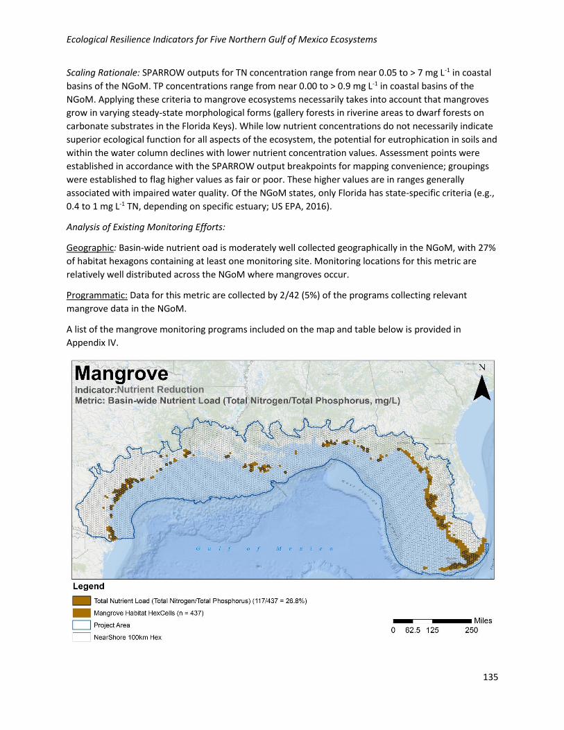
Ecological Resilience Indicators for Five Northern Gulf of Mexico Ecosystems
135
Scaling Rationale: SPARROW outputs for TN concentration range from near 0.05 to > 7 mg L-1 in coastal
basins of the NGoM. TP concentrations range from near 0.00 to > 0.9 mg L-1 in coastal basins of the
NGoM. Applying these criteria to mangrove ecosystems necessarily takes into account that mangroves
grow in varying steady-state morphological forms (gallery forests in riverine areas to dwarf forests on
carbonate substrates in the Florida Keys). While low nutrient concentrations do not necessarily indicate
superior ecological function for all aspects of the ecosystem, the potential for eutrophication in soils and
within the water column declines with lower nutrient concentration values. Assessment points were
established in accordance with the SPARROW output breakpoints for mapping convenience; groupings
were established to flag higher values as fair or poor. These higher values are in ranges generally
associated with impaired water quality. Of the NGoM states, only Florida has state-specific criteria (e.g.,
0.4 to 1 mg L-1 TN, depending on specific estuary; US EPA, 2016).
Analysis of Existing Monitoring Efforts:
Geographic: Basin-wide nutrient oad is moderately well collected geographically in the NGoM, with 27%
of habitat hexagons containing at least one monitoring site. Monitoring locations for this metric are
relatively well distributed across the NGoM where mangroves occur.
Programmatic: Data for this metric are collected by 2/42 (5%) of the programs collecting relevant
mangrove data in the NGoM.
A list of the mangrove monitoring programs included on the map and table below is provided in
Appendix IV.
Nutrient Reduction
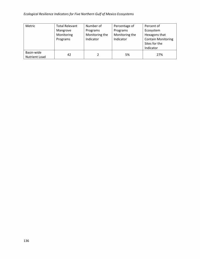
Ecological Resilience Indicators for Five Northern Gulf of Mexico Ecosystems
136
Metric Total Relevant Mangrove Monitoring Programs
Number of Programs Monitoring the Indicator
Percentage of Programs Monitoring the Indicator
Percent of Ecosystem Hexagons that Contain Monitoring Sites for the Indicator
Basin-wide Nutrient Load
42 2 5% 27%
Ecological Resilience Indicators for Five Northern Gulf of Mexico Ecosystems
137
Indicator: Soil Carbon Storage
MES: Regulating
KES: Carbon Sequestration
Metric: Mangrove Height
Definition: Soil carbon storage is the quantity of carbon stored in the soil. Mangrove height is a good
indicator of ecosystem productivity and soil carbon storage.
Background: Coastal wetland ecosystems (i.e., salt marshes, mangroves, and seagrass beds) can store
large quantities of carbon in the soil because of high rates of above- and belowground primary
production (carbon input), relatively low rates of decomposition (carbon export), and accretionary (i.e.,
soil burial) processes due to rising sea levels (Chmura et al., 2003; Donato et al., 2011; Mcleod et al.,
2011). Mangrove ecosystems fix (or sequester) large amounts of carbon dioxide (CO2) in the soil. Soil
carbon in flooded and anaerobic wetland soils decompose more slowly, because anaerobic respiration is
less efficient than aerobic respiration. Therefore, the potential for long-term storage of carbon in
wetland soils is significant and much greater than most terrestrial ecosystems.
Rationale for Selection of Variable: In mangrove ecosystems, there is often a positive relationship
between plant height and plant productivity (Komiyama et al., 2008; Castañeda-Moya et al., 2011;
Castañeda-Moya et al., 2013). At the scale of the Gulf of Mexico, which spans many environmental
gradients that affect carbon storage, plant height can serve as a proxy for productivity and soil carbon
accumulation. Since data for these latter two rates (i.e., carbon accumulation and productivity) are often
not readily available, plant height is a valuable indicator that can be used to coarsely characterize and
quickly assess the potential for carbon storage in mangrove ecosystems.
Measure: Mangrove plant height (m)
Tier: 3 (intensive field measurement)
Measurement: There are many approaches for measuring height. Height measurements could be
conducted in the field and/or via remotely-sensed approaches.
Metric Rating and Assessment Points:
Metric Rating Mangrove Height
Excellent > 2 m
Good 1–2 m
Fair < 1 m
Scaling Rationale: Carbon storage potential is high in almost all mangroves. Hence, the excellent rating
in the greater than 2 m height category and the good rating in the 1 to 2 m height category. Carbon
storage is only likely to be low in ecosystems where an abiotic factor (e.g., hypersalinity, oligotrophic
conditions, excessive inundation) limits mangrove development and productivity. In these systems,
mangroves are likely to be short (i.e., less than 1 m in height).
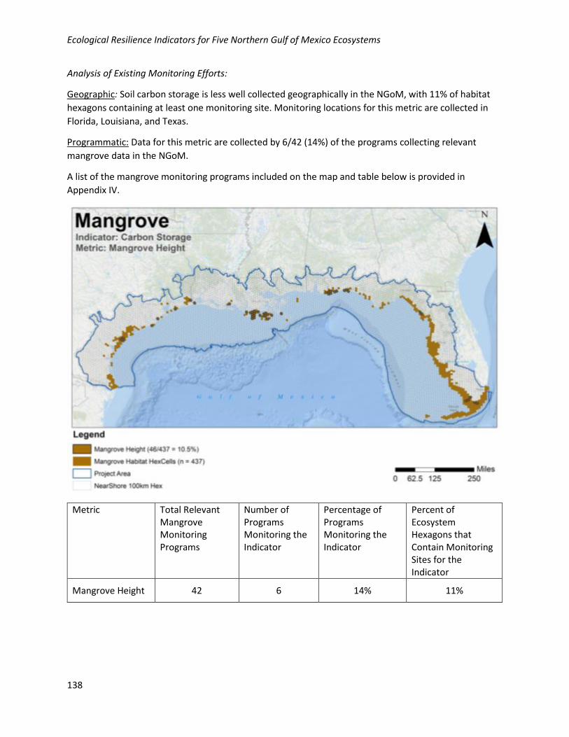
Ecological Resilience Indicators for Five Northern Gulf of Mexico Ecosystems
138
Analysis of Existing Monitoring Efforts:
Geographic: Soil carbon storage is less well collected geographically in the NGoM, with 11% of habitat
hexagons containing at least one monitoring site. Monitoring locations for this metric are collected in
Florida, Louisiana, and Texas.
Programmatic: Data for this metric are collected by 6/42 (14%) of the programs collecting relevant
mangrove data in the NGoM.
A list of the mangrove monitoring programs included on the map and table below is provided in
Appendix IV.
Metric Total Relevant Mangrove Monitoring Programs
Number of Programs Monitoring the Indicator
Percentage of Programs Monitoring the Indicator
Percent of Ecosystem Hexagons that Contain Monitoring Sites for the Indicator
Mangrove Height 42 6 14% 11%

Ecological Resilience Indicators for Five Northern Gulf of Mexico Ecosystems
139
Indicator: Recreational Fishery
MES: Cultural
KES: Aesthetics-Recreational Opportunities
Metric: Density of Juvenile Common Snook
This metric is the same as used for the Status of Macrofauna Population indicator above.
Definition: Number of individuals of juvenile (standard length [SL] <= 10 in) common snook
(Centropomus undecimalis), per unit area.
Background: Snook are subtropical euryhaline fishes with a strong preference for mangrove estuarine
habitats. Of the five species that occur in Florida, common snook (Centropomus undecimalis) is the most
common and popular inshore game fish in Florida (see other species:
http://myfwc.com/research/saltwater/fish/snook/sketch-common-snook/). In the NGoM, they occur
just north of Tampa Bay, covering the densely mangrove-populated coast line. Juvenile snook are found
between freshwater rivers to mangrove-fringed estuarine coast until they reach about 10 to 14 inches
long. After this, they reach sexual maturity and move to higher-salinity areas of the estuaries. Their
habitat preference lies in the common characteristics of mangrove forest habitat of good water quality,
moderate slope in banks, slow currents, overhanging vegetation that provides shade, and the structure
that is provided by the mangrove root system (Seaman and Collins, 1983). Snook are fished year-round
in Florida, and its recreational fishery is regulated in state and federal waters. No commercial harvest or
sale of snook is permitted at this point.
Rationale for Selection of Variable: Density constitutes an important statistic to describe and understand
wild populations. It allows for the assessment of population resource utilization at a specific habitat. The
measurement of density is relevant when dealing with resident small fish and invertebrates when the
goal is to assess complex areas (Beck et al., 2001) and where visual census is not suitable.
Measure: Individuals per square meter. Field-collected organisms should be identified and enumerated.
Tier: 3 (intensive field measurement)
Measurement: Use standard methods for fish census. Record all organisms and data should be
presented on individuals/m2. Conduct field measures at different areas of the estuaries such as
upstream and downstream where the salinity gradient is different.
Metric Rating and Assessment Points:
Metric Rating Density of Juvenile* Common Snook (Centropomus undecimalis)
Upstream (ponds and creeks mean) Downstream (ponds and creeks mean)
Good–Excellent >= 7.0 fish/100m2 or stable/increasing >= 2.6 fish/100m2 or stable/increasing
Poor < 7.0 fish/100m2 or decreasing < 2.6 fish/100m2 or decreasing
*Ratings here are provided for young of the year fish < 150 mm SL.
Scaling Rationale: The fish densities used were estimated by Brame (2012) in the study of juvenile
common snook along mangrove shoreline in Frog Creek, a tidal tributary of Tampa Bay, Florida. Density
values above the published mean from Brame (2012) are considered good to excellent population
health. Fish densities below are considered poor. Densities at different salinity gradients—i.e., upstream
Ecological Resilience Indicators for Five Northern Gulf of Mexico Ecosystems
140
and downstream estuarine areas—are presented. Since the available assessment points are available
from only one study, if densities vary significantly from the suggested values, employ the
stable/increasing/decreasing metric ratings instead.
Analysis of Existing Monitoring Efforts:
No programs in the monitoring program inventory specifically noted collection of common snook.
Spatial data from Frog Creek study were not available.
Ecological Resilience Indicators for Five Northern Gulf of Mexico Ecosystems
141
References
Avery, M.L., J.S. Humphrey, K.L. Keacher, and W.E. Bruce, 2014. Detection and Removal of Invasive
Burmese Pythons: Methods Development Update. Edited by R.M. Timm and J.M. O’Brien. Proceedings of
the 26th Veterbrate Pest Conference. University of California, Davis, CA, USA. 145–148.
Barbier, E.B., E.W. Koch, B.R. Silliman, S.D. Hacker, E. Wolanski, J. Primavera, E.F. Granek, S. Polasky, S.
Aswani, L.A. Cramer, D. Stoms, C.J. Kennedy, D. Bael, C.V. Kappel, G.M.E. Perillo, and D.J. Reed, 2008.
Coastal ecosystem-based management with non-linear ecological functions and values. Science 319:
321–323.
Barbier, E.B. and M. Cox, 2003. Does economic development lead to mangrove loss? A cross-country
analysis. Contemporary Economic Policy 21: 418–432.
Barbier, E.B., S.D. Hacker, C. Kennedy, E.W. Koch, A. Stier, and B.R. Silliman, 2011. The value of estuarine
and coastal ecosystem services. Ecological Monographs 81(2): 169–193.
Barbour, A.B., M.L. Montgomery, A.A. Adamson, E. Díaz-Ferguson, and B.R. Silliman, 2010. Mangrove
use by the invasive lionfish Pterois volitans. Marine Ecology Progress Series 401: 291–294.
Bellis, V. and A. Gaither, 1985. Salt Marsh Productivity Studies: A Project Status Report to North Carolina
Phosphate Corp., Aurora, NC, Sea-level rise as a cause of shore erosion." Journal Waterways and
Harbors Division, ASCE 88.
Beck, M.W., K.L. Heck, Jr., K.W. Able, D.L. Childers, D.B. Eggleston, B.M. Gillanders, B. Halpern, C.G. Hays,
K. Hoshino, T.J. Minello, R.J. Orth, P.F. Sheridan, and M.P. Weinstein, 2001. The identification,
conservation, and management of estuarine and marine nurseries for fish and invertebrates: A better
understanding of the habitats that serve as nurseries for marine species and the factors that create site-
specific variability in nursery quality will improve conservation and management of these
areas. BioScience 51(8): 633–641.
Betts, T., 2006. An assessment of mangrove cover and forest structure in Las Perlas, Panama. Master’s
Thesis. Heriot Watt University, Edinburgh, Scotland.
Bird Watcher’s Digest, 2017. 10 Highlight Birds in Florida.
(https://www.birdwatchersdigest.com/bwdsite/explore/regions/southeast/florida/10-birds-florida.php)
Accessed online July 28, 2017.
Brame, A.B., 2012. An Ecological Assessment of a Juvenile Estuarine Sportfish, Common Snook
(Centropomus undecimalis), in a Tidal Tributary of Tampa Bay, Florida. Graduate Thesis and
Dissertations. University of South Florida. St. Petersburg, 197 pages.
Bouillon, S., A.V. Borges, E. Castañeda‐Moya, K. Diele, T. Dittmar, N.C. Duke, E. Kristensen, S.Y. Lee, C.
Marchand, J.J. Middelburg, and V.H. Rivera‐Monroy, 2008. Mangrove production and carbon sinks: A
revision of global budget estimates. Global Biogeochemical Cycles 22(2).
Ecological Resilience Indicators for Five Northern Gulf of Mexico Ecosystems
142
Brinson, M.M., 1993. Changes in the functioning of wetlands along environmental gradients. Wetlands
13: 65–74. doi:10.1007/BF03160866.
Burton, M.L., 2001. Age, growth, and mortality of gray snapper, Lutjanus griseus, from the east coast of
Florida. Fishery Bulletin 99: 254–265.
Cahoon, D.R., 2015. Estimating relative sea-level rise and submergence potential at a coastal wetland.
Estuaries Coasts 38: 1077–1084. doi:10.1007/s12237-014-9872-8.
Cahoon, D.R., J.C. Lynch, P. Hensel, R. Boumans, B.C. Perez, B. Segura, and J.W. Day, 2002a. High-
precision measurements of wetland sediment elevation: I. Recent improvements to the sedimentation-
erosion table. Journal of Sediment Research 72: 730–733. doi:10.1306/020702720730.
Cahoon, D.R., J.C. Lynch, B.C. Perez, B. Segura, R.D. Holland, C. Stelly, G. Stephenson, and P. Hensel,
2002b. High-precision measurements of wetland sediment elevation: II. The rod surface elevation table.
Journal of Sediment Research 72: 734–739. doi:10.1306/020702720734.
Cahoon, D.R. and R.E. Turner, 1989. Accretion and canal impacts in a rapidly subsiding wetland II.
Feldspar marker horizon technique. Estuaries 12: 260–268. doi:10.2307/1351905.
Castañeda-Moya, E., R.R. Twilley, and V.H. Rivera-Monroy, 2013. Allocation of biomass and net primary
productivity of mangrove forests along environmental gradients in the Florida Coastal Everglades, USA.
Forest Ecology and Management 307: 226–241.
Castañeda-Moya, E., R.R. Twilley, V.H. Rivera-Monroy, B.D. Marx, C. Coronado-Molina, and S.M. Ewe,
2011. Patterns of root dynamics in mangrove forests along environmental gradients in the Florida
Coastal Everglades, USA. Ecosystems 14: 1178–1195.
Cavanaugh, K.C., J.R. Kellner, A.J. Forde, D.S. Gruner, J.D. Parker, W. Rodriguez, and I.C. Feller, 2014.
Poleward expansion of mangroves is a threshold response to decreased frequency of extreme cold
events. Proceedings of the National Academy of Sciences 111: 723–727.
Chambers, L.G., T.Z. Osborne, and K.R. Reddy, 2013. Effect of salinity-altering pulsing events on soil
organic carbon loss along an intertidal wetland gradient: A laboratory
experiment. Biogeochemistry 115(1–3): 363-383.
Chapin, F.S., P.A. Matson, and H.A. Mooney, 2002. Principles of Terrestrial Ecosystem Ecology. Springer,
New York, NY, USA.
Chen, G., B. Chen, D. Yu, N.F. Tam, Y. Ye, and S. Chen, 2016. Soil greenhouse gas emissions reduce the
contribution of mangrove plants to the atmospheric cooling effect. Environmental Research
Letters 11(12): 124019.
Childers, D.L. and J.W. Day, 1990. Marsh-water column interactions in two Louisiana estuaries. I.
Sediment dynamics. Estuaries 13: 393–403. doi:10.2307/1351784.
Ecological Resilience Indicators for Five Northern Gulf of Mexico Ecosystems
143
Chmura, G.L., 2013. What do we need to assess the sustainability of the tidal salt marsh carbon sink?
Ocean & Coastal Management 83: 25e31.
Chmura, G.L., S.C. Anisfeld, D.R. Cahoon, and J.C. Lynch, 2003. Global carbon sequestration in tidal,
saline wetland soils. Global Biogeochemical Cycles 17: 1111.
Coastal Blue Carbon, 2015. Available from: https://www.estuaries.org/bluecarbon.
Comeaux, R.S., M.A. Allison, and T.S. Bianchi, 2012. Mangrove expansion in the Gulf of Mexico with
climate change: Implications for wetland health and resistance to rising sea levels. Estuarine, Coastal
and Shelf Science 96: 81–95.
Costanza, R., O. Perez-Maqueo, M.L. Martinez, P. Sutton, S.J. Anderson, and K. Mulder, 2008. The value
of coastal wetlands for hurricane protection. Ambio 37(4): 241–248.
Couvillion, B.R., M.R. Fischer, H.J. Beck, and W.J. Sleavin, 2016. Spatial configuration trends in coastal
Louisiana from 1985 to 2010. Wetlands 1–13. doi:10.1007/s13157-016-0744-9.
Culbertson, J.B., I. Valiela, M. Pickart, E.E. Peacock., and C.M. Reddy, 2008. Long-term consequences of
residual petroleum on salt marsh grass. Journal of Applied Ecology 45(4): 1284–1292.
Danielsen, F., M.K. Sorensen, M.F. Olwig, V. Selvam, F. Parish, N.D. Burgess, T. Hiraishi, V.M.
Karunagaran, M.S. Rasmussen, L.B. Hansen, A. Quarto, and N. Suryadiputra, 2005. The Asian tsunami: A
protective role for coastal vegetation. Science 310(5748): 643.
Das, S. and J.R. Vincent, 2009. Mangroves protected villages and reduced death toll during Indian super
cyclone. Proceedings of the National Academy of Sciences of the United States of America 106(40):
7357–7360.
Davis, W.P., S.D. Taylor, and B.J. Turner, 1995. Does the autecology of the mangrove rivulus fish (Rivulus
marmoratus) reflect a paradigm for mangrove ecosystem sensitivity? Bulletin of Marine Science 57(1):
208–214.
Day, J.W., C.A.S. Hall, W.M. Kemp, and A. Yáñez-Arancibia, 1989. Estuarine Ecology. John Wiley & Sons,
Inc., New York.
Day, J.W., C. Coronado-Molina, F.R. Vera-Herrera, R. Twilley, V.H. Rivera-Monroy, H. Alvarez-Guillen, R.
Day, and W. Conner, 1996. A 7-year record of above-ground net primary production in a southeastern
Mexican mangrove forest. Aquatic Botany 55(1): 39–60.
Day, J.W., A. Yáñez-Arancibia, J.H. Cowan, R.H. Day, R.R. Twilley, J.R. Rybczyk, 2013. Global Climate
Change Impacts on Coastal Ecosystems in the Gulf of Mexico: Considerations for Integrated Coastal
Management. In: Day, J.W. and A. Yáñez-Arancibia (editors). Gulf of Mexico Origin, Waters, and Biota
Volume 4: Ecosystem-based Management. Harte Research Institute for Gulf of Mexico Studies, Texas A
& M University-Corpus Christi, Texas A&M University Press.
Ecological Resilience Indicators for Five Northern Gulf of Mexico Ecosystems
144
Deegan, L.A., D.S. Johnson, R.S. Warren, B.J. Peterson, J.W. Fleeger, S. Fagherazzi, and W.M. Wollheim,
2012. Coastal eutrophication as a driver of salt marsh loss. Nature 490: 388–392.
doi:10.1038/nature11533.
DeLaune, R.D., W.H. Patrick, R.J. Buresh, 1979. Effect of crude oil on a Louisiana Spartina alterniflora salt
marsh. Environmental Pollution 20: 21–31. doi:10.1016/0013-9327(79)90050-8.
Delgado, P., P.F. Hensel, J.A. Jiménez, and J.W. Day, 2001. The importance of propagule establishment
and physical factors in mangrove distributional patterns in a Costa Rican estuary. Aquatic Botany 71(3):
157–178.
Diop, E.S., A. Soumare, N. Diallo, and A. Guisse, 1997. Recent changes of the mangroves of the Saloum
River Estuary, Senegal. Mangroves and Salt Marshes 1: 163–172.
Donato, D.C., J.B. Kauffman, D. Murdiyarso, S. Kurnianto, M. Stidham, and M. Kanninen, 2011.
Mangroves among the most carbon-rich forests in the tropics. Nature Geoscience 4: 293–297.
Eslami-Andargoli, L., P. Dale, N. Sipe, and J. Chaseling, 2009. Mangrove expansion and rainfall patterns in
Moreton Bay, southeast Queensland, Australia. Estuarine, Coastal and Shelf Science 85: 292–298.
Ewel, K.C., R.R. Twilley, and J.E. Ong, 1998. Different kinds of mangrove forests provide different goods
and services. Global Ecology and Biogeography Letters 7: 83–94.
Fagherazzi, S., G. Mariotti, P. Wiberg, and K. McGlathery, 2013. Marsh collapse does not require sea
level rise. Oceanography 26: 70–77. doi:10.5670/oceanog.2013.47.
Feher, L.C., M.J. Osland, and K.T. Griffith, et al., 2017. Linear and nonlinear effects of temperature and
precipitation on ecosystem properties in tidal saline wetlands. Ecosphere 8: Article e01956.
Feller, I.C., 1995. Effects of nutrient enrichment on growth and herbivory of dwarf red mangrove
(Rhizophora mangle). Ecological Monographs 65: 477–505.
Feller, I.C., K.L. McKee, D.F. Whigham, and J.P. O'Neill, 2003. Nitrogen vs. phosphorus limitation across
an ecotonal gradient in a mangrove forest. Biogeochemistry 62: 145–175.
Feller, I.C., C. Lovelock, and K.L. Mckee, 2007. Nutrient addition differentially affects ecological
processes of Avicennia germinans in nitrogen versus phosphorus limited mangrove ecosystems.
Ecosystems 10: 347–359.
Fourqurean, J.W., T.J. Smith III, J. Possley, T.M. Collins, D. Lee, and S. Namoff, 2010. Are mangroves in
the tropical Atlantic ripe for invasion? Exotic mangrove trees in the forests of South Florida. Biological
Invasions 12: 2509–2522.
Gabler, C.A., M.J. Osland, and J.B. Grace, et al., 2017. Macroclimatic change expected to transform
coastal wetland ecosystems this century. Nature Climate Change 7: 142–147.
Ecological Resilience Indicators for Five Northern Gulf of Mexico Ecosystems
145
Gilman, E.L., J. Ellison, N.C. Duke, and C. Field, 2008. Threats to mangroves from climate change and
adaptation options: A review. Aquatic Botany 89(2): 237–250.
Gilmore, R.G., C.J. Donohoe, and D.W. Cooke, 1983. Observations on the distribution and biology of
east-central Florida populations of the common snook, Centropomus undecimalis (Bloch). Florida
Scientist 46: 313–336.
GMFMC, 2011. Final Generic Annual Catch Limits/Accountability Measures Amendment for the Gulf of
Mexico Fishery Management Council’s Red Drum, Reef Fish, Shrimp, Coral and Coral Reefs, Fishery
Management Plans. GMFMC, Tampa, FL. September 2011.
Gulf of Mexico Fishery Management Council, 1981. Environmental impact statement and fishery
management plan for the reef fish resources of the Gulf of Mexico. National Marine Fishery Service.
Tampa, 328 pages.
Guntenspergen, G.R., D.R. Cahoon, J. Grace, G.D. Steyer, S. Fournet, M.A. Townson, and A.L. Foote,
1995. Disturbance and recovery of the Louisiana coastal marsh landscape from the impacts of Hurricane
Andrew. Journal of Coastal Research SI 21: 324–339.
Hare, J.A., M.J. Wuenschel, and M.E. Kimball, 2012. Projecting range limits with coupled thermal
tolerance - Climate change models: An example based on gray snapper (Lutjanus griseus) along the U.S.
East coast. PLoS ONE 7(12): e52294.
Hatton, R.S., R.D. DeLaune, and W.H.J. Patrick, 1983. Sedimentation, accretion, and subsidence in
marshes of Barataria Basin, Louisiana. Limnology and Oceanography 28(3): 494–502.
Holling, C.S., 1973. Resilience and stability of ecological systems. Annual Review of Ecological Systems 4:
1–23.
Hunter, M.E., S.J. Oyler-McCance, R.M. Dorazio, J.A. Fike, B.J. Smith, C.T. Hunter, R.N. Reed, and K.M.
Hart, 2015. Environmental DNA (eDNA) sampling improves occurrence and detection estimates of
invasive Burmese pythons. PloS ONE 10(4): e0121655.
Kadlec, R.H., 1990. Overland flow in wetlands: Vegetation resistance. Journal of Hydraulic Engineering
116: 691–706. doi:10.1061/(ASCE)0733-9429(1990)116:5(691).
Kennish, M.J., 2001. Coastal salt marsh systems in the U.S.: A review of anthropogenic impacts. Journal
of Coastal Research 17: 731–748.
Kirwan, M.L. and J.P. Megonigal, 2013. Tidal wetland stability in the face of human impacts and sea-level
rise. Nature 504: 53–60. doi:10.1038/nature12856.
Knight, J.M., L. Griffin, P.E. Dale, and M. Sheaves, 2013. Short-term dissolved oxygen patterns in sub-
tropical mangroves. Estuarine, Coastal and Shelf Science 131: 290–296.
Koch, E.W., E.B. Barbier, B.R. Silliman, D.J. Reed, G.M. Perillo, S.D. Hacker, E.F. Granek, J.H. Primavera, N.
Muthiga, S. Polasky, B.S. Halpern, C.J. Kennedy, C.V. Kappel, and E. Wolanski, 2009. Non-linearity in
Ecological Resilience Indicators for Five Northern Gulf of Mexico Ecosystems
146
ecosystem services: Temporal and spatial variability in coastal protection. Frontiers in Ecology and the
Environment 7(1): 29–37.
Komiyama, A., J.E. Ong, and S. Poungparn, 2008. Allometry, biomass, and productivity of mangrove
forests: A review. Aquatic Botany 89: 128–137.
Krauss, K.W., T.W. Doyle, R.R. Twilley, V.H. Rivera-Monroy, and J.K. Sullivan, 2006. Evaluating the
relative contributions of hydroperiod and soil fertility on growth of south Florida
mangroves. Hydrobiologia 569(1): 311–324.
Krauss, K.W., C.E. Lovelock, K.L. McKee, L. López-Hoffman, S.M. Ewe, and W.P. Sousa, 2008.
Environmental drivers in mangrove establishment and early development: A review. Aquatic
Botany 89(2): 105–127.
Krauss, K.W., K.L. McKee, C.E. Lovelock, D.R. Cahoon, N. Saintilan, R. Reef, and L. Chen, 2014. How
mangrove forests adjust to rising sea level. New Phytologist 202:19–34.
Laegdsgaard, P. and C. Johnson, 2001. Why do juvenile fish utilize mangrove habitats? Journal of
Experimental Marine Biology and Ecology 257(2): 229–253.
Law, B.E. and N.A. Pywell, 1988. Mangroves-Florida’s coastal trees forest resources and conservation.
Fact Sheet FRC-43. University of Florida, Cooperative Extension Service/Institute of Food and
Agricultural Sciences, 4 pages.
Lee, S.Y., 1995. Mangrove outwelling: A review. Hydrobiologia 295(1–3): 203–212.
Leslie, D.M., Jr., 2016. An International Borderland of Concern—Conservation of Biodiversity in the
Lower Rio Grande Valley: U.S. Geological Survey Scientific Investigations Report 2016–5078, 120 pages.
http://dx.doi.org/10.3133/sir20165078.
Lewis, R.R., E.C. Milbrandt, B. Brown, K.W. Krauss, A.S. Rovai, J.W. Beever, and L.L. Flynn, 2016. Stress in
mangrove forests: Early detection and preemptive rehabilitation are essential for future successful
worldwide mangrove forest management. Marine pollution Bulletin 109: 764–771.
Lovelock, C.E., 2008. Soil respiration and belowground carbon allocation in mangrove
forests. Ecosystems 11(2): 342–354.
Lovelock, C.E., M.C. Ball, K.C. Martin, and I.C. Feller, 2009. Nutrient enrichment increases mortality of
mangroves. PLoS ONE 4(5): e5600.
Lugo, A.E. and S.C. Snedaker, 1974. The ecology of mangroves. Annual Review of Ecology and
Systematics 5: 39–64.
Luo, J., J.E. Serafy, S. Sponaugle, P.B. Teare, and D. Kieckbusch, 2009. Movement of gray snapper
Lutjanus griseus among subtropical seagrass, mangrove, and coral reef habitats. Marine Ecology
Progress Series 380: 255–269.
Ecological Resilience Indicators for Five Northern Gulf of Mexico Ecosystems
147
Maher, D.T., I.R. Santos, L. Golsby-Smith, J. Gleeson, and B.D. Eyre, 2013. Groundwater‐derived
dissolved inorganic and organic carbon exports from a mangrove tidal creek: The missing mangrove
carbon sink? Limnology and Oceanography 58(2): 475–488.
Marois, D.E. and W.J. Mitsch, 2015. Coastal protection from tsunamis and cyclones provided by
mangrove wetlands–a review. International Journal of Biodiversity Science, Ecosystem Services &
Management 11: 71–83.
Marshall, A.R., 1958. A survey of the snook fishery of Florida, with studies of the biology of the principal
species, Centropomus undecimalis (Bloch). Florida Board of Conservation Marine Research Laboratory,
Technical Series Report 22.
McIvor, A.L., T. Spencer, I. Möller, and M. Spalding, 2012. Storm surge reduction by mangroves. Natural
Coastal Protection Series: Report 2. Cambridge Coastal Research Unit Working Paper 41. Published by
The Nature Conservancy and Wetlands International.
McIvor, C.C. and T.J. Smith, 1995. Differences in the crab fauna of mangrove areas at a southwest Florida
and a northeast Australia location: Implications for leaf litter processing. Estuaries 18(4): 591–597.
McKee, K.L., I.C. Feller, M. Popp, and W. Wanek, 2002. Mangrove isotopic fractionation (15N and 13C)
across a nitrogen versus phosphorus limitation gradient. Ecology 83: 1065–1075.
McKee, K.L., D.R. Cahoon, and I.C. Feller, 2007. Caribbean mangroves adjust to rising sea level through
biotic controls on change in soil elevation. Global Ecology and Biogeography 16(5): 545–556.
Mcleod, E., G.L. Chmura, and S. Bouillon, et al., 2011. A blueprint for blue carbon: Toward an improved
understanding of the role of vegetated coastal habitats in sequestering CO2. Frontiers in Ecology and the
Environment 9: 552–560.
McMillan, C. and C.L. Sherrod, 1986. The chilling tolerance of black mangrove, Avicennia germinans,
from the Gulf of Mexico coast of Texas, Louisiana, and Florida. Contributions in Marine Science 29: 9–16.
Milliman, J.D. and R.H. Meade, 1983. World-wide delivery of river sediment to the oceans. The Journal
of Geology 91: 1–21.
Millennium Ecosystem Assessment, 2005. Ecosystems and human well-being: Biodiversity synthesis.
World Resource Institute, Washington, DC, 86 pages.
Mitsch, W.J. and J.G. Gosselink, 2015. Wetlands, 5th ed. John Wiley & Sons, Inc., Hoboken, NJ, USA.
Morris, J.T., D.C. Barber, J.C. Callaway, R. Chambers, S.C. Hagen, C.S. Hopkinson, B.J. Johnson, P.
Megonigal, S.C. Neubauer, T. Troxler, and C. Wigand, 2016. Contributions of organic and inorganic
matter to sediment volume and accretion in tidal wetlands at steady state. Earths Future 4: 110–121.
doi:10.1002/2015EF000334.
Neubauer, S.C., 2008. Contributions of mineral and organic components to tidal freshwater marsh
accretion. Estuarine, Coastal and Shelf Science 78: 78–88. doi:10.1016/j.ecss.2007.11.011.
Ecological Resilience Indicators for Five Northern Gulf of Mexico Ecosystems
148
Osland, M.J., N. Enwright, R.H. Day, and T.W. Doyle, 2013. Winter climate change and coastal wetland
foundation species: salt marshes vs. mangrove forests in the southeastern United States. Global Change
Biology 19: 1482–1494.
Osland, M.J., N. Enwright, and C.L. Stagg, 2014. Freshwater availability and coastal wetland foundation
species: Ecological transitions along a rainfall gradient. Ecology 95: 2789–2802.
Osland, M.J., R.H. Day, A.S. From, M.L. McCoy, J.L. McLeod, and J.J. Kelleway, 2015. Life stage influences
the resistance and resilience of black mangrove forests to winter climate extremes. Ecosphere 6(9): 1–
15.
Osland, M.J., N.M. Enwright, R.H. Day, C.A. Gabler, C.L. Stagg, and J.B. Grace, 2016. Beyond just sea-level
rise: Considering macroclimatic drivers within coastal wetland vulnerability assessments to climate
change. Global Change Biology 22: 1–11.
Pendleton, E.A., J.A. Barras, S.J. Williams, and D.C. Twichell, 2010. Coastal Vulnerability Assessment of
the Northern Gulf of Mexico to Sea-Level Rise and Coastal Change (USGS Open-File Report No. 2010–
1146).
Preston, S.D., R.B. Alexander, G.E. Schwarz, and C.G. Crawford, 2011. Factors affecting stream nutrient
loads: A synthesis of regional SPARROW model results for the continental United States. JAWRA Journal
of the American Water Resources Association 47: 891–915. doi:10.1111/j.1752-1688.2011.00577.x.
Rutherford, E.S., J.T. Tilmant, E.B. Thue, and T.W. Schmidt, 1989. Fishery harvest and population
dynamics of gray snapper, Lutjanus griseus, in Florida Bay and adjacent waters. Bulletin of Marine
Science 44(1): 139–154.
Saintilan, N., N.C. Wilson, K. Rogers, A. Rajkaran, and K.W. Krauss, 2014. Mangrove expansion and salt
marsh decline at mangrove poleward limits. Global Change Biology 20: 147–157.
Scharler, U.M., R.E. Ulanowicz, M.L. Fogel, M.J. Wooller, M. Jacobson-Meyers, C.E. Lovelock, I.C. Feller,
M. Frischer, R. Lee, K. McKee, I.C. Romero, J.P. Schmit, and C. Shearer, 2015. Variable nutrient
stoichiometry (carbon:nitrogen:phosphorus) across trophic levels determines community and
ecosystem properties in an oligotrophic mangrove system. Oecologia 179: 863–876.
Scyphers, S.B., S.P. Powers, J.L. Akins, J.M. Drymon, C.W. Martin, Z.H. Schobernd, P.J. Schofield, R.L.
Shipp, and T.S. Switzer, 2015. The role of citizens in detecting and responding to a rapid marine
invasion. Conservation Letters 8(4): 242–250.
Seaman, Jr., W. and M. Collins, 1983. Species profiles: Life histories and environmental requirements of
coastal fishes and invertebrates (South Florida): Snook. No. 82/11.16. US Fish and Wildlife Service.
Smith, V.H., 2003. Eutrophication of freshwater and coastal marine ecosystems a global
problem. Environmental Science and Pollution Research 10(2): 126–139.
Ecological Resilience Indicators for Five Northern Gulf of Mexico Ecosystems
149
Smith III, T.J., G.H. Anderson, K. Balentine, G. Tiling, G.A. Ward, and K.R. Whelan, 2009. Cumulative
impacts of hurricanes on Florida mangrove ecosystems: Sediment deposition, storm surges and
vegetation. Wetlands 29: 24–34.
Spalding, M., M. Kainuma, and L. Collins, 2010. World Atlas of Mangroves. Earthscan. London, 319
pages.
Stagg, C.L., K.W. Krauss, D.R. Cahoon, N. Cormier, W.H. Conner, and C.M. Swarzenski, 2016. Processes
contributing to resilience of coastal wetlands to sea-level rise. Ecosystems 1–15.
Stagg, C.L., L. Sharp, T.E. McGinnis, and G.A. Snedden, 2013. Submergence Vulnerability Index
Development and Application to Coastwide Reference Monitoring System Sites and Coastal Wetlands
Planning, Protection and Restoration Act Projects (USGS Open-File Report No. 2013–1163).
Stuart, S.A., B. Choat, K.C. Martin, N.M. Holbrook, and M.C. Ball, 2007. The role of freezing in setting the
latitudinal limits of mangrove forests. New Phytologist 173(3): 576–583.
Suzuki, T., M. Zijlema, B. Burger, M.C. Meijer, and S. Narayan, 2012. Wave dissipation by vegetation with
layer schematization in SWAN. Coastal Engineering 59(1): 64–71.
The Nature Conservancy, 2017. Measures guidebook for flood and storm risk reduction projects. The
Nature Conservancy, Arlington, VA, 78 pages.
Tiner, R.W., 2013. Tidal Wetlands Primer: An Introduction to their Ecology, Natural History, Status, and
Conservation. University of Massachusetts Press, Amherst and Boston, 508 pages.
Tobias, S., 1995. Shear strength of the soil-root bond system. In: Telford, T. (editor). Vegetation and
Slopes: Stabilisation, Protection and Ecology: Proceedings of the International Conference Held at the
University Museum, Oxford, 29–30 September 1994.
Tockner, K., D. Pennetzdorfer, N. Reiner, F. Schiemer, and J.V. Ward, 1999. Hydrological connectivity,
and the exchange of organic matter and nutrients in a dynamic river–floodplain system (Danube,
Austria). Freshwater Biology 41: 521–535. doi:10.1046/j.1365-2427.1999.00399.x.
Tomlinson, P.B., 1986. The Botany of Mangroves. Cambridge University Press.
Trexler, J.C., W.F. Loftus, F. Jordan, J.L. Lorenz, J.H. Chick, and R.M. Kobza, 2000. Empirical assessment of
fish introductions in a subtropical wetland: an evaluation of contrasting views. Biological Invasions 2:
265–277.
Turner, R.E., 2010. Beneath the salt marsh canopy: Loss of soil strength with increasing nutrient loads.
Estuaries Coasts 34: 1084–1093. doi:10.1007/s12237-010-9341-y.
Twilley, R.R., R.H. Chen, and T. Hargis, 1992. Carbon sinks in mangroves and their implications to carbon
budget of tropical coastal ecosystems. Water, Air, and Soil Pollution 64: 265–288.
Ecological Resilience Indicators for Five Northern Gulf of Mexico Ecosystems
150
UNEP, 2014. The Importance of Mangroves to People: A Call to Action. van Bochove, J., E. Sullivan, and T.
Nakamura (editors). UNEP World Conservation Monitoring Centre, Cambridge, 128 pages.
US EPA, 2016. State-Specific Water Quality Standards Effective Under the Clean Water Act (CWA).
https://www.epa.gov/wqs-tech/state-specific-water-quality-standards-effective-under-clean-water-act-
cwa.
USFS Forest Inventory and Analysis, 2011. Section 23: Crowns: Measurements and Sampling. Phase 3
National Core Field Guide, version 5.1. US Department of Agriculture, US Forest Service.
https://www.fia.fs.fed.us/library/field-guides-methods-proc/docs/2012/field_guide_p3_5-
1_sec23_10_2011.pdf.
USFWS [U.S. Fish and Wildlife Service], 2016. National Wetlands Inventory website. U.S. Department of
the Interior, Fish and Wildlife Service, Washington, DC. http://www.fws.gov/wetlands/.
USNVC [United States National Vegetation Classification], 2016. United States National Vegetation
Classification Database, V2.0. Federal Geographic Data Committee, Vegetation Subcommittee,
Washington DC. www.usnvc.org. Accessed 23 Sept 2016.
Ward, R.D., D.A. Friess, R.H. Day, R.A. MacKenzie, 2016. Impacts of climate change on mangrove
ecosystems: A region by region overview. Ecosystem Health and Sustainability 2(4): e01211.
doi:10.1002/ehs2.1211.
Woodroffe, C.D., K. Rogers, K.L. McKee, C.E. Lovelock, I.A. Mendelssohn, N. Saintilan, 2016. Mangrove
sedimentation and response to relative sea-level rise. Annual Review of Marine Science 8: 243–266.
Wright, L.D, 1977. Sediment transport and deposition at river mouths: A synthesis. Geological Society of
America Bulletin 88: 857–868. doi:10.1130/0016-7606(1977)88<857:STADAR>2.0.CO;2.
Yoskowitz, D., C. Santos, B. Allee, C. Carollo, J. Henderson, S. Jordan, and J. Ritchie, 2010. Proceedings of
the Gulf of Mexico Ecosystem Services Workshop: Bay St. Louis, Mississippi, June 16–18, 2010. Harte
Research Institute for Gulf of Mexico Studies, Texas A&M University-Corpus Christi, 16 pages.