CHAPTER 3

3 DYNAMIC DEFLECTION MONITORING OF EPS EMBANKMENT TO

SUPPORT RAILWAY SYSTEM

3.1 Introduction

The amount of deflection of the rail caused by the passing of a locomotive or rail car is

a significant safety issue for rail system operations. Large deflections could pose the risk

of possible derailment, especially at higher speeds of operation. Dynamic rail deflections

can occur on all types of embankment support systems.

The amount of deflection can be measured by using direct or indirect methods. For

direct methods, measurement is usually done by via survey equipment, lasers, or other

optical equipment (e.g., high-speed cameras) deployed in the field. When optical

techniques are used, optical equipment are used to obtain images, and those images are

subsequently processed to determine relative displacement. For indirect methods, the

amount deflection is measured either by instrumentation and numerical interpretation. The

most common indirect method involves the installation of accelerometers or geophones at

the site. These sensors can provide time history data of acceleration or velocity. This

information can be integrated to provide estimates of displacement of the rail versus time.

The use of optical techniques to measure the dynamic deflection on rails and sleepers

that atop the embankment made from conventional materials have been carried out by

2

several researchers (Ho et al., 2006; Bowness et al., 2007; Lu, 2008; Pinto et al., 2009;

Psimoulis and Stiros, 2013). The video graphic and image processing techniques were used

to monitor the vertical displacements of rail sleepers with the passage of trains by Ho et al.

(2006). Bowness et al. (2007) monitored the dynamic displacement of railway track using

remote video monitoring system. Lu (2008) developed a system to measure track deflection

from a moving railcar. The system was comprised of a loaded hopper car fitted with a

camera/lesser sensor system which detected the vertical deflection of the rail relative to the

wheel/rail contact point. Pinto et al. (2009) used an optical system for monitoring the

vertical displacements of the track in high speed railways. The system was based on a diode

laser module mounted away from the track. Psimoulis and Stiros (2013) measured the

deflection of a short-span railway bridge using robotic total station (RTS).

The use of indirect methods to measure the dynamic deflection in the field have been

carried out by several researchers (Madshus and Kaynia, 2000; Bowness et al., 2007;

Chebli et al., 2008; Priest and Powrie, 2009; Ling et al., 2010). Madshus and Kaynia (2000)

studied the motions of the track and embankment by installing the accelerometers in the

field. In this study the displacement was calculated and the results were compared with

numerical simulation. Bowness et al. (2007) monitored the dynamic deflection of railway

tracks by placing the geophones on the sleepers. The field test results were then compared

with the results obtained from an optical target method. Chebli et al. (2008) studied the

dynamic response of high-speed ballasted railway tracks using a three dimensional (3D)

periodic model and in-situ measurement. As an in-situ measurement, accelerometers were

installed at various locations to measure the vertical acceleration and displacement. In this

method, the accelerometers were placed on the sleepers. The in-situ measurement results

3

were then compared with the results obtained from 3D periodic model. Priest and Powrie

(2009) evaluated the dynamic track modulus by measuring track velocity during train

passage. In this method, geophones were attached to the sleeper outside the rail. Dynamic

displacement was calculated from the measured velocity. Ling et al. (2010) studied train

induced vibration response characteristics and dynamic stability of track structures by

installing accelerometers on sleepers, rail and embankment slopes.

The use of EPS geofoam for railway embankments has not been studied to any great

extent. O'Brien (2001) described the innovative solution for the replacement of an old

railway bridge by using EPS geofoam embankment in United Kingdom (UK). From this

study, one can understand the potential of using EPS geofoam as a lightweight fill material

for railway embankment for short term and long term purposes. So far, there are no study

focusing exclusively on vertical deflection monitoring of EPS embankment to support

railway system. (WHAT ABOUT THE STUDY OF DEFLECTION IN NORWAY

REFERENCED IN SHUN’S THESIS).

In the United States, EPS geofoam was recently incorporated in portions of the

commuter and light rail systems in Salt Lake City, Utah by the Utah Transit Authority

(UTA). The FrontRunner commuter rail south line extends from Salt Lake City to Provo,

Utah. Along this line at Corner Canyon in Draper City, EPS has been used in the

embankment in order to minimize the stress over a reinforced concrete box culvert. This

location has both EPS geofoam and adjacent earthen embankment. Similarly, the light rail

line (Green Line) extends from West Valley Central to Salt Lake City International Airport.

In this line, EPS has been used in the embankment near Roper Yard, which is operated by

4

the Union Pacific Railroad. These two sites were selected to monitor the dynamic

deflections of EPS geofoam embankment.

The main objectives of the study were to: (1) develop an optical technique to measure

the dynamic vertical deflection, (2) evaluate the performance of the developed optical

technique, (3) measure the vertical deflection during passage of trains using accelerometers

and (4) compare the results of vertical deflection of EPS embankment with that of the

earthen embankment.

3.2 Field Description

The FrontRunner commuter rail system in the Corner Canyon area in Draper City, Utah

has rail embankment constructed of both EPS geofoam and conventional fill materials. The

site is shown in Figure 3.1. This system consists of (from top to bottom): steel rail, ballast,

sub-ballast, concrete reinforcing slab, EPS geofoam and sand. The slope of an embankment

is 2H:1V. The cross-section of an embankment is shown in Figure 3.2. Similarly, a photo

of the EPS embankment used to support light rail along Green Line near River Trail is

shown in Figure 3.3. (SHOULD INCLUDE A X-SECTION OF THIS EMBANKMENT

ALSO, SIMILAR TO THAT USED IN FIGURE 3.2).

5

Figure 3.1. Embankment with EPS geofoam and conventional fill materials in Draper city of Utah along FrontRunner line

Figure 3.2. Cross-section of an EPS geofoam embankment at corner canyon of Draper city of Utah

6

Figure 3.3. EPS embankment to support light rail along Green Line near River Trail of Utah

3.3 Equipment and Methods

3.3.1 Dynamic Deflection Monitoring

In the study, an optical target technique was developed for measuring the dynamic

deflection of the rail, but this techniques was not deployed in the field due to poor weather

conditions (high winds). However, an accelerometer array was installed in the field and

the data from these were interpreted to provide estimates of rail deflections.

3.3.1.1 Development of Optical Technique

In this method, a paper target (Figure 3.4) was developed and used for laboratory

testing of the system and optical interpretation. The target was attached on a wooden frame

and kept on the MTS machine as shown. The MTS machine has an actuator that can be

controlled to produce a systematic and controlled vertical displacement. A LVDT was used

to measure the linear displacement versus time. A loading protocol was set up in the MTS

7

machine for cyclic loading of a frequency 0.5 Hz and peak to peak amplitude of 7 mm. The

protocol was written to yield time and displacement as output.

Figure 3.4. Target set-up on MTS machine

Bowness et al. (2007) considered the minimum distance between target and camera to

be 10 m in order to minimize the effects of train vibration on the camera. This

recommendation was used for this study, where video was recorded by setting a Go-ProTM

camera and telescope at a 10-m distance from the target as shown in Figure 3.5. The Go-

ProTM camera was able to take pictures and videos at a rate of 120 frames per second, and

had a Wi-Fi system which could connected to another electronic devices to display the

target. The target was made with black and white squares in order to make analysis easier.

After recording the video, an image processing technique was employed to find the vertical

deflection.

8

In this method, the video recordings were converted into several still frames. The first

frame was taken as the base image. The center of the target was determined in terms of

pixel number for each frames. The displaced position of center of the target in the vertical

direction was determined in terms of pixels and was converted into linear distance.

For the analysis, an algorithm was developed in MATLAB. The algorithm is given in

Appendix A. In this process, all images were uploaded initially. The central black square

box of the target was chosen as the region of interest. The region was selected to make sure

that the total displacement of the square still remains within the peripheral white region. A

matrix was created with zeros in all rows and columns. The region of interest was then

replaced by the matrix with zero values. Therefore, this region became completely different

from the peripheral zones. A histogram was made for the linearly spaced vectors, which

were prepared from a one-dimensional (1D) matrix. The 1D matrix was obtained from the

rows and columns of the selected region. The threshold value of the pixels in the region

was then determined. Values smaller than threshold were made zero. Similarly, values

greater than threshold were set equal to one.

Figure 3.5. Camera-telescope set up for video recording

9

The total number of rows where the values were non zero represented the length of the

square. Thus, the total number of pixels along the length of one small square was

determined. The identity of the center region was then determined in terms of its pixel

number. The pixel numbers for the center region of subsequent images were determined in

similar manner. Once the minimum pixel numbers were determined, then each pixel

number was subtracted from this. (The pixel numbers represented the distance in terms of

the number of pixels from the minimum value.) A linear scale was used to measure the side

of the big square. The total number of pixels at one side of the big square were also

calculated. A conversion factor was determined for converting pixels into corresponding

linear displacement. The time was calculated by dividing the frames to the number of

frames in one second. For example, if there were 200 frames in 10 seconds then the 20

frames were obtained in 1 second. From this, a plot was made between displacement and

time. The total displacement was then determined from the plot. The displacement versus

time from both optical techniques and data extracted from MTS machine was plotted on

the same graph for comparison (Figure 3.6).

10

Figure 3.6. Comparison of displacement obtained from image processing in optical technique and LVDT measurement in MTS machine

After laboratory verification, a similar instrument was developed for field

implementation. At the Corner Canyon embankment site, there is no level ground around

for a distance of 10 m from the target on the rail to where the embankment slope begins.

The embankment slopes away from the rail on a 2H:1V side slope. Therefore in order to

measure the deflection on sloped ground, a modification of the set-up was introduced. A

telescoping rod was fixed on a survey tripod, and the telescope with a Go-ProTM camera

was mounted at the top of the rod. The rod and camera attached was able to rotate (Figure

3.7). The target could be seen using a Wi-Fi device such as smart phone or tablet using the

Wi-Fi system of the Go-ProTM camera. Unfortunately, however, this technique proved to

be very sensitive to vibration for wind and other ambient sources.

11

Figure 3.7. Optical technique instrument set up for field measurement of vertical deflection

3.3.2 Accelerometers for Dynamic Deflection Monitoring

Five accelerometers of model 4630A (Figure 3.8) were used in the sites for deflection

monitoring. The triaxial accelerometers were cubical in shape with dimension of 25.4 mm.

The dynamic range of the accelerometers was 100g to2g with an operating

temperature of -550c to 1250c. Data from the accelerometers were collected at a sampling

interval of 1 x 10-3 sec (1000 Hz). The accelerometers were glued on the concrete tie (i.e.,

sleeper) to measure the deflection. Figure 3.9 shows the orientation of the accelerometer

on the sleeper.

12

Figure 3.8. Model 4630A accelerometer

Figure 3.9. Accelerometer glued on sleeper with its orientation

As shown in Figure 3.9, the Z axis was oriented along the vertical direction, the Y axis

was parallel to the rail and the X axis was perpendicular to the rail. The spacing between

the accelerometers were installed using the live load configuration provided by American

Railway Engineering and Maintenance-of-Way Association (AREMA) manual (AREMA,

2007) for the train locomotive (Figure 3.10).

13

Figure 3.10. Axial load configurations for locomotive and cars with position of accelerometers at A, B and C (AREMA, 2007) for FrontRunner

Figure 3.11. Accelerometers positions at A, B and C along light rail line In Figure 3.10, the letters A, B and C denote the position of the accelerometers. The

maximum axle load was exerted by a locomotive is 75 K (kips). The configuration of

accelerometers was chosen in such a way that the maximum load could be recorded by the

sensors. Similarly, Figure 3.11 shows the positioning of accelerometers at A, B and C in

the sleepers along the light rail line. A similar orientation and positioning was used for the

light rail measurements.

The FrontRunner train had three double decker passenger cars, one single decker car

and a locomotive as shown in Figure 3.12 (locomotive is shown at far left of photo). The

14

train is southbound in this case and is enroute to Provo, Utah. The light train had two cars

as shown in Figure 3.13.

Figure 3.12. Front runner heading towards south on the route with three double deck cars, one single deck car and a locomotive

Figure 3.13. Light rail heading towards the West Valley Central with two passenger cars

Two accelerometers were glued at positions A and B where the maximum axle load

would be exerted on the sleeper. A third accelerometer was glued at position C which lied

in between A and B. The accelerometers were then connected to the data logger to extract

data. The data logger to be used in the instrumentation was CR9000X is shown in Figure

15

3.14. The basic CR9000X system consists of CR9011 power supply module, a CR9032

CPU module and CR9052DC Anti-Alias Filter Module with DC Excitation.

Figure 3.14. CR9000X measurement and control system with CR9052DC Anti-Alias filter modulus and DC excitation

The filter module connector has a number of channels. Each input channel consists of

both regulated constant voltage excitation (VEX) and regulated constant current excitation

(IEX) channels. There are five ports for excitation with high voltage input, low voltage

input, return and ground. Each accelerometer has five colored wires namely: red, green,

white, black and silver and were connected to the five ports on data loggers: excitation

(VEX or IEX), high side of the differential voltage input (VIN+), low side of the

differential voltage input (VIN-), return (VRTN or IRTN) and ground respectively.

16

The RTDAQTM (Real-time Data Acquisition) software was used for the collection of

data and was connected to the USB serial port. In RTDAQ, there are three tabs for

operation: clock/program, monitor data and collect data. The recorded time in the data

logger and pc was synchronized by using the update and check button. The monitor data

tab is important for the collection of data. It consists of a ports and flags window. In this

window, the flag should be turned on during collection of data. The green light on flag

denotes the flag is turned on. Once the train approached the embankment, the flag was

turned on. Shortly after the train passed through the embankment array, this flag was turned

off.

The data between time of flag being turned on and being turned off was recorded. The

collection data tab was used for data collection. In this tab, there are three collection

options: collect mode, file mode and file format. All the data options were used in the

collect mode. In the file mode and file format, append to end of file and ASCII table data

were selected. The start collection tab was used for the collection of data.

After data collection, the next step consisted of the analysis of the field accelerometer

data. This was done using the commercially available software SeismoSignalTM. This

software has filtering and baseline correction routines which can be used to convert the

input acceleration time history to velocity and displacement time histories.

The collected data was impacted by high frequency noise (i.e., vibration) which created

spurious baseline errors. Therefore, the baseline correction and frequency filtering features

of this software were employed to re-baseline the measurements and to remove unwanted

high frequency signal. The available baseline corrections methods were: constant, linear,

quadratic and cubic. For this study, the linear baseline correction function was chosen

17

because it provided the most reasonable adjustment to the trend in the data. After

completing the base line correction, Fourier and power spectra were plotted for each of the

train events. The Fourier amplitude spectrum shows the distribution of amplitude of

motion with frequency and the power spectrum reveals the power spectral density with

respect to frequency. The frequency band for filtering was determined based on plots of

the Fourier and power spectrum (Figure 3.16). These plots suggest that much of the signal

above about 60 Hz is high frequency noise from vibration, which is not of interest for

estimating the deflection of the rail from the moving train.

In addition, the SeismoSignalTM software has four types of filter configurations:

lowpass, highpass, bandpass and bandstop. For the creation of the filter configurations,

three filter types are available: Butterworth, Chebyshev and Bessel filters. In this study, a

Butterworth filter type was used which featured a flat response in the pass band. The

Bandpass filtering configuration was applied in the study which allows signals to pass

through the given frequency range. The lower frequency in the Bandpass was chosen to be

large (10 seconds) based on the time required during the passage of the train and the high

frequency was selected based on the frequency and power spectrum plots (Figure 3.16).

The baseline corrected and filtered time series provides records of the acceleration, velocity

and displacement time history of the rail ties. The vertical displacement of the tie was used

to estimate the vertical deflection of the rail because there little opportunity for relative

vertical movement between the rail and the rail ties.

18

3.4 Results from Field Measurements

3.4.1 Optical Technique

The results from the test of the laboratory optical technique matched well with the MTS

results. This proved that the optical technique, as developed, was able to give reliable

results in controlled conditions. However, subsequently this technique was not deployed in

the field due to field geometrical constraints and weather conditions. The technique so

developed for the field did not perform to its fullest capacity because the study site was

windy during the field testing. In addition, it was not possible to gain additional access to

the site at a later date when more favorable weather conditions might have prevailed due

to the time limits placed on the deflection monitoring by the UTA track access permit.

Therefore, the technique was not used for field measurements at the Corner Canyon site.

Nonetheless, the developed technique and algorithm may be useful for future projects

or for laboratory measurements for cases where the ambient conditions are more favorable.

In short, the optical technique presents a very low cost alternative when compared with the

expense required to deploy an accelerometer array and its corresponding high-speed data

acquisition system; hence because of this, the optical technique merits further consideration

and development.

3.4.2 Accelerometer Array

The orientation of the accelerometers and their locations are shown in Figures 3.9 and

3.11. The possible influence that filtering might have on the vertical displacement results

was studied by using various values for the upper frequency of the band pass filter. The

estimated displacement time history corresponding to an upper band pass frequency of 30,

60 and 90 Hz are shown in Figure 3.15. This parametric change revealed that the selected

19

displacement record was not significantly altered by the selection of the high frequency for

the band pass filter.

The displacement results from the accelerometers positioned at points A, B and C in

the EPS embankments for the along commuter rail line and light rail lines are described

separately in the following sections.

3.4.2.1 Commuter Rail Line

The Fourier amplitude and power spectra of the recorded data from accelerometers

positioned at A, B and C were analyzed in order to finalize the filtering process and to

select the upper frequency in the band pass filtering. The Fourier amplitude and power

spectrum of A, B and C positions are shown in Figures 3.16, 3.17 and 3.18, respectively.

Figure 3.15. Vertical displacement record using different levels for the upper frequency in the Bandpass filter

20

(a)

(b)

Figure 3.16. The record of accelerometer at position A along commuter rail line (a) Fourier amplitude and (b) Power spectrum

21

(a)

(b)

Figure 3.17. The record of accelerometer at position B along commuter rail line (a) Fourier amplitude and (b) Power spectrum

22

(a)

(b)

Figure 3.18. The record of accelerometer at position C along commuter rail line (a) Fourier amplitude and (b) Power spectrum

23

Based on these plots, it was concluded that the average value of frequency beyond

which significant noise started was about 70 Hz in both the Fourier amplitude and power

spectra. Thus, the highest upper frequency for the band pass filter to selected to be 70 Hz.

The time taken for trains to pass the sensors was less than 10 sec and the lowest level of

frequency to be considered was 0.1 Hz.

The train bound to Salt Lake City from Provo will be referred to as the north bound

(NB) train, and that bound from Salt Lake to Provo will be referred to as the south bound

(SB) train hereafter. The train shown in Figure 3.10 was a SB train. In the study, three NB

trains named 1, 2 and 3 were monitored for estimating the vertical deflection of rail atop

EPS embankment. Three NB trains were named 4, 5 and 6 were monitored for the

determination of vertical deflection of rail atop earthen embankment. The accelerometers

were placed on the sleepers adjacent to the NB train track; whereas the SB train track was

located 1.5 m distance from the position of the accelerometers. The NB trains were used

for measuring vertical deflection because the vertical stress on embankments was assumed

to be higher under the NB train track due to the placement of the accelerometers directly

on this track. However, one NB and one SB train were monitored to compare the results in

terms of the vertical deflections.

The input acceleration and the vertical displacement of three trains on EPS

embankment are shown in Figures 3.19, 3.20 and 3.21. Figure 3.19 reveals the input

acceleration and the vertical displacement measured by the accelerometer at position A due

to trains 1, 2 and 3. In Figure 3.19, a somewhat higher peak displacement occurred at the

beginning of the record when the train had just entered over the EPS embankment at about

8 seconds of elapsed time. The maximum displacement for this spike was found to be 6

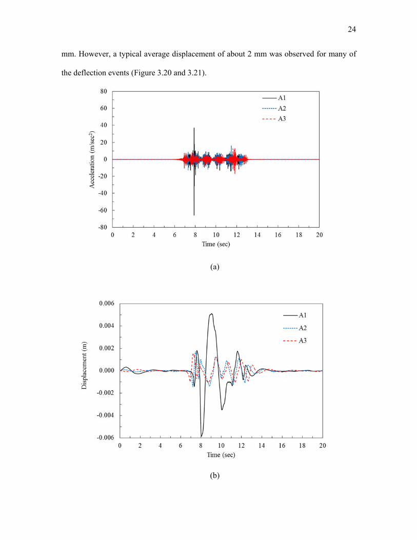
24

mm. However, a typical average displacement of about 2 mm was observed for many of

the deflection events (Figure 3.20 and 3.21).

(a)

(b)

25

Figure 3.19. The record of accelerometer position at A of EPS embankment along commuter rail line (a) Input acceleration and (b) Vertical displacement

(a)

(b)

26

Figure 3.20. The record of accelerometer position at B of EPS embankment along commuter rail line (a) Input acceleration and (b) Vertical displacement

(a)

(b)

27

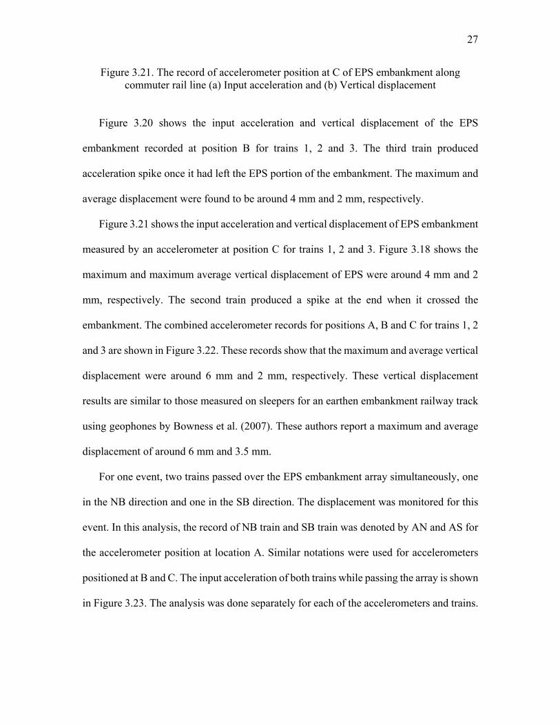
Figure 3.21. The record of accelerometer position at C of EPS embankment along commuter rail line (a) Input acceleration and (b) Vertical displacement

Figure 3.20 shows the input acceleration and vertical displacement of the EPS

embankment recorded at position B for trains 1, 2 and 3. The third train produced

acceleration spike once it had left the EPS portion of the embankment. The maximum and

average displacement were found to be around 4 mm and 2 mm, respectively.

Figure 3.21 shows the input acceleration and vertical displacement of EPS embankment

measured by an accelerometer at position C for trains 1, 2 and 3. Figure 3.18 shows the

maximum and maximum average vertical displacement of EPS were around 4 mm and 2

mm, respectively. The second train produced a spike at the end when it crossed the

embankment. The combined accelerometer records for positions A, B and C for trains 1, 2

and 3 are shown in Figure 3.22. These records show that the maximum and average vertical

displacement were around 6 mm and 2 mm, respectively. These vertical displacement

results are similar to those measured on sleepers for an earthen embankment railway track

using geophones by Bowness et al. (2007). These authors report a maximum and average

displacement of around 6 mm and 3.5 mm.

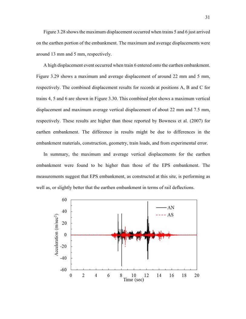
For one event, two trains passed over the EPS embankment array simultaneously, one

in the NB direction and one in the SB direction. The displacement was monitored for this

event. In this analysis, the record of NB train and SB train was denoted by AN and AS for

the accelerometer position at location A. Similar notations were used for accelerometers

positioned at B and C. The input acceleration of both trains while passing the array is shown

in Figure 3.23. The analysis was done separately for each of the accelerometers and trains.

28

29

Comparative plots of the input acceleration and vertical displacements of the EPS

embankment recorded by accelerometers A, B and C are shown in Figures 3.24, 3.25 and

3.26, respectively.

Figure 3.22. Vertical displacement recorded by accelerometers at positions A, B and C for trains 1, 2 and 3 in the EPS embankment along commuter rail line

30

Figure 3.23. The input acceleration of NB and SB train while simultaneously crossing the EPS embankment along commuter rail line

These figures show that the maximum and average vertical displacements for the NB

train are about 4 mm and 1.5 mm, respectively; whereas about 1 mm and 0.75 mm was

recorded for the SB train, respectively. The lower values for the SB train was due to its

greater distance from the position of the accelerometer array placed on the NB rail.

The input acceleration and vertical displacements for three train events named as 4, 5

and 6 on the adjacent earthen embankments are shown in Figures 3.27, 3.28 and 3.29,

respectively. Figure 3.27 shows the maximum displacement occurred when the train 4 just

entered this portion of the embankment. There was an initial displacement spike at the

beginning of this passing, followed by lower displacements a few seconds afterward. The

maximum and maximum average displacements were about 12 mm and 3 mm, respectively

for the earthen embankment.

31

Figure 3.28 shows the maximum displacement occurred when trains 5 and 6 just arrived

on the earthen portion of the embankment. The maximum and average displacements were

around 13 mm and 5 mm, respectively.

A high displacement event occurred when train 6 entered onto the earthen embankment.

Figure 3.29 shows a maximum and average displacement of around 22 mm and 5 mm,

respectively. The combined displacement results for records at positions A, B and C for

trains 4, 5 and 6 are shown in Figure 3.30. This combined plot shows a maximum vertical

displacement and maximum average vertical displacement of about 22 mm and 7.5 mm,

respectively. These results are higher than those reported by Bowness et al. (2007) for

earthen embankment. The difference in results might be due to differences in the

embankment materials, construction, geometry, train loads, and from experimental error.

In summary, the maximum and average vertical displacements for the earthen

embankment were found to be higher than those of the EPS embankment. The

measurements suggest that EPS embankment, as constructed at this site, is performing as

well as, or slightly better that the earthen embankment in terms of rail deflections.

32

(a)

(b)

Figure 3.24. The comparative plot of record on EPS embankment by accelerometer at position A (a) Input acceleration and (b) Vertical displacement

(a)

33

(b)

Figure 3.25. The comparative plot of record on EPS embankment by accelerometer at position B (a) Input acceleration and (b) Vertical displacement

(a)

34

(b)

Figure 3.26. The comparative plot of record on EPS embankment by accelerometer at position C (a) Input acceleration and (b) Vertical displacement

(a)

35

(b)

Figure 3.27. The record of accelerometer position at A of earthen embankment along commuter rail line (a) Input acceleration and (b) Vertical displacement

(a)

36

(b)

Figure 3.28. The record of accelerometer position at B of earthen embankment along commuter rail line (a) Input acceleration and (b) Vertical displacement

(a)

37

(b)

Figure 3.29. The record of accelerometer position at C of earthen embankment along commuter rail line (a) Input acceleration and (b) Vertical displacement

38

Figure 3.30. Vertical displacement recorded by accelerometers at positions A, B and C for trains 4, 5 and 6 in the earthen embankment along commuter rail line

3.4.2.2 Light Rail Line Array

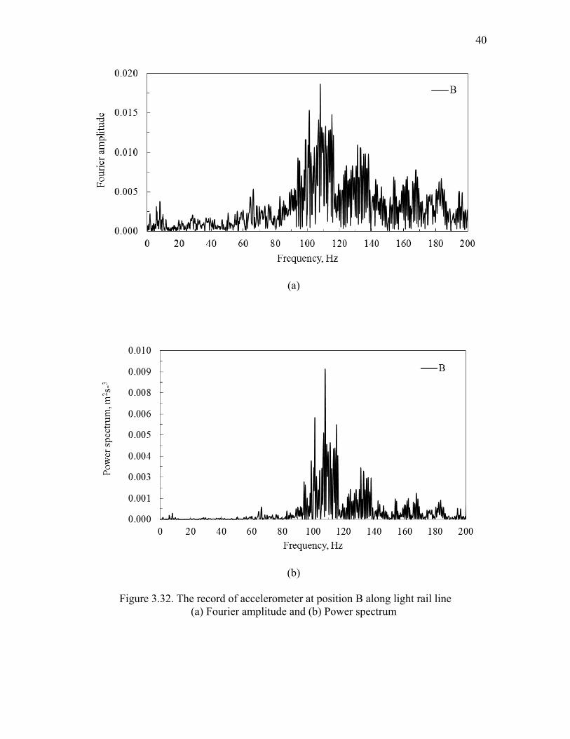
The Fourier amplitude and power spectrum for the A, B and C positions are shown in

Figures 3.31, 3.32 and 3.33, respectively, for the UTA light rail system (i.e., TRAX). The

average frequency beyond which significant noise started was about 80 Hz for both Fourier

amplitude and power spectrum. Thus, the highest frequency considered in the data

interpretation was 80 Hz. The time taken for trains to pass the sensors was less than 10 sec

and the lowest level of frequency to be considered was 0.1 Hz.

39

(a)

(b)

Figure 3.31. The record of accelerometer at position A along light rail line (a) Fourier amplitude and (b) Power spectrum

40

(a)

(b)

Figure 3.32. The record of accelerometer at position B along light rail line (a) Fourier amplitude and (b) Power spectrum

41

(a)

(b)

Figure 3.33. The record of accelerometer at position C along light rail line

(a) Fourier amplitude and (b) Power spectrum

42

The westbound (WB) train bound to West Valley Central Station from Salt Lake City

International Airport was monitored for this study. The train from the West Valley Central

Station to Airport will be referred to as the east bound (EB) train hereafter. The train shown

in Figure 3.13 is the WB train. In this study, five WB trains named as 1, 2, 3, 4 and 5 were

monitored for the determination of the vertical deflection of concrete rail ties (i.e., sleepers)

constructed atop a large EPS embankment. The WB train were selected for the monitoring

and the accelerometers were placed on the sleepers for the WB rail. At this location, the

EB track was about 1.5 m distance from the position of the accelerometers on the WB rail.

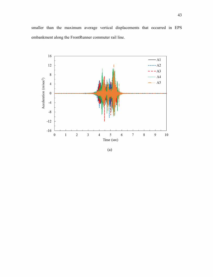
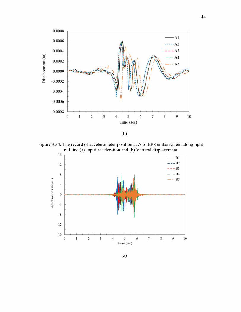
The acceleration time histories and the vertical displacement of five trains traveling on

the EPS embankment are shown in Figures 3.34, 3.35 and 3.36. Figure 3.34 shows the input

acceleration and the vertical displacements estimated by the accelerometer at position A

due to trains 1, 2 3, 4 and 5. The process of converting the acceleration time history to

displacement was the same as that used for the FrontRunner system, discussed previously,

except the upper frequency for the band pass filter was set to 80 Hz. In Figure 3.34, the

maximum displacement was estimated to be about 0.6 mm. Figure 3.35 shows the input

acceleration and vertical displacement of the EPS embankment recorded for the position

of accelerometer at B for trains 1, 2, 3, 4 and 5. The maximum displacement was about 0.5

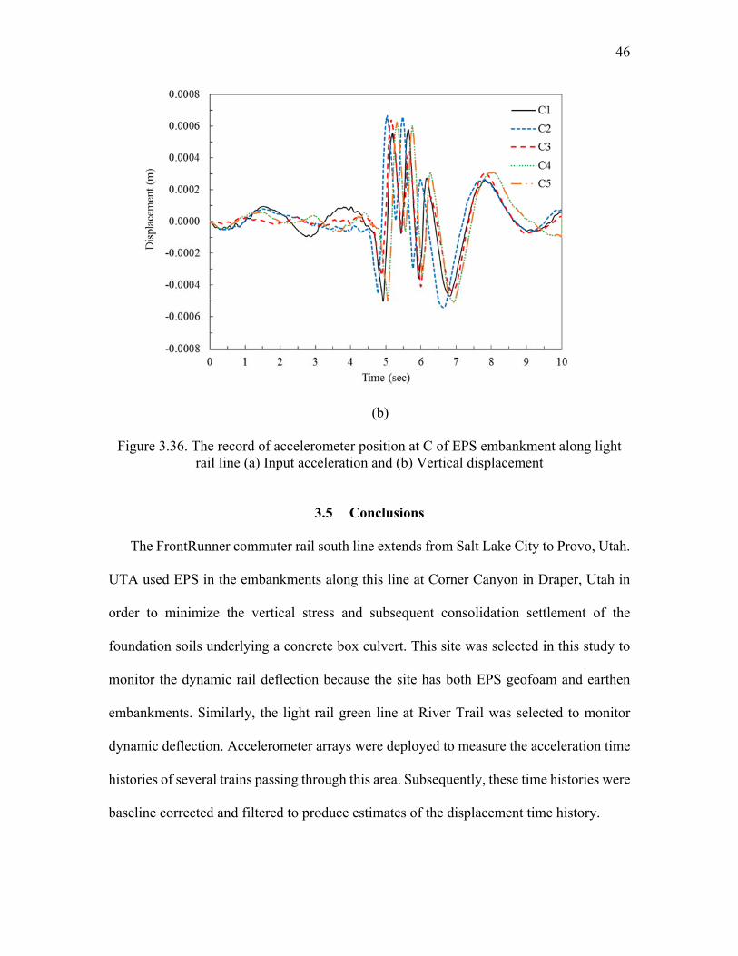
mm. Figure 3.36 shows the input acceleration and vertical displacement of the EPS

embankment measured by accelerometer at position C for trains 1, 2, 3, 4 and 5. Figure

3.34 shows the maximum vertical displacement of EPS was about 0.7 mm.

The records on accelerometers at positions A, B and C for trains 1, 2, 3, 4 and 5 show

the average vertical displacements were about 0.6 mm. This value is approximately 4 times

43

smaller than the maximum average vertical displacements that occurred in EPS

embankment along the FrontRunner commuter rail line.

(a)

44

(b)

Figure 3.34. The record of accelerometer position at A of EPS embankment along light rail line (a) Input acceleration and (b) Vertical displacement

(a)

45

(b)

Figure 3.35. The record of accelerometer position at B of EPS embankment along light rail line (a) Input acceleration and (b) Vertical displacement

(a)

46

(b)

Figure 3.36. The record of accelerometer position at C of EPS embankment along light rail line (a) Input acceleration and (b) Vertical displacement

3.5 Conclusions

The FrontRunner commuter rail south line extends from Salt Lake City to Provo, Utah.

UTA used EPS in the embankments along this line at Corner Canyon in Draper, Utah in

order to minimize the vertical stress and subsequent consolidation settlement of the

foundation soils underlying a concrete box culvert. This site was selected in this study to

monitor the dynamic rail deflection because the site has both EPS geofoam and earthen

embankments. Similarly, the light rail green line at River Trail was selected to monitor

dynamic deflection. Accelerometer arrays were deployed to measure the acceleration time

histories of several trains passing through this area. Subsequently, these time histories were

baseline corrected and filtered to produce estimates of the displacement time history.

47

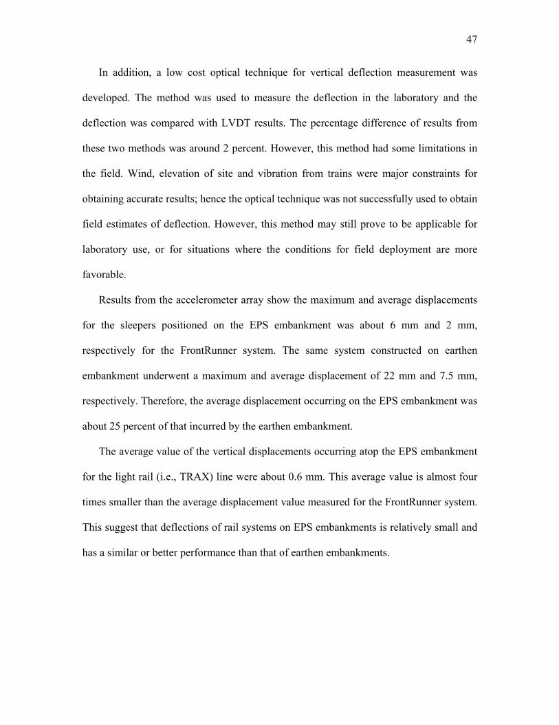
In addition, a low cost optical technique for vertical deflection measurement was

developed. The method was used to measure the deflection in the laboratory and the

deflection was compared with LVDT results. The percentage difference of results from

these two methods was around 2 percent. However, this method had some limitations in

the field. Wind, elevation of site and vibration from trains were major constraints for

obtaining accurate results; hence the optical technique was not successfully used to obtain

field estimates of deflection. However, this method may still prove to be applicable for

laboratory use, or for situations where the conditions for field deployment are more

favorable.

Results from the accelerometer array show the maximum and average displacements

for the sleepers positioned on the EPS embankment was about 6 mm and 2 mm,

respectively for the FrontRunner system. The same system constructed on earthen

embankment underwent a maximum and average displacement of 22 mm and 7.5 mm,

respectively. Therefore, the average displacement occurring on the EPS embankment was

about 25 percent of that incurred by the earthen embankment.

The average value of the vertical displacements occurring atop the EPS embankment

for the light rail (i.e., TRAX) line were about 0.6 mm. This average value is almost four

times smaller than the average displacement value measured for the FrontRunner system.

This suggest that deflections of rail systems on EPS embankments is relatively small and

has a similar or better performance than that of earthen embankments.

48

3.6 References

AREMA (2007). "Manual for Railway Engineering." American Railway Engineering and Maintenance-of Way Association, Lanham, Maryland, USA.

Bowness, D., Lock, A., Powrie, W., Priest, J., and Richards, D. "Monitoring the dynamic

displacements of railway track." Proc., Institution of Mechanical Engineers, Part F: Journal of Rail and Rapid Transit, 13-22.

Chebli, H., Clouteau, D., and Schmitt, L. (2008). "Dynamic response of high-speed

ballasted railway tracks: 3D periodic model and in situ measurements." Soil Dynamics and Earthquake Engineering, 28(2), 118-131.

Ho, S., Tsang, W., Lee, K., Lee, K., Lai, W., Tam, H., and Ho, T. "Monitoring of the

vertical movements of rail sleepers with the passage of trains." Proc., Institution of Engineering and Technology International Conference on Railway Condition Monitoring, 2006, IEEE, 108-114.

Ling, X.-Z., Chen, S.-J., Zhu, Z.-Y., Zhang, F., Wang, L.-N., and Zou, Z.-Y. (2010). "Field

monitoring on the train-induced vibration response of track structure in the Beiluhe permafrost region along Qinghai–Tibet railway in China." Cold Regions Science and Technology, 60(1), 75-83.

Lu, S. (2008). "Real-time vertical track deflection measurement system." Ph.D. thesis,

University of Nebraska, Lincoln, Nebraska, USA. Madshus, C., and Kaynia, A. (2000). "High-speed railway lines on soft ground: dynamic

behaviour at critical train speed." Journal of Sound and Vibration, 231(3), 689-701. O'Brien, A. (2001). "Design and construction of the UK's first polysterene embankment

for railway use." Proc., 3rd International EPS Geofoam Conference, Salt Lake City, Utah, USA.

Pinto, N., Ribeiro, C., Mendes, J., and Calçada, R. (2009). "An optical system for

monitoring the vertical displacements of the track in high speed railways." Proc., 3rd International Integrity Reliability and Failure, Portugal, 1-9.

Priest, J., and Powrie, W. (2009). "Determination of dynamic track modulus from

measurement of track velocity during train passage." Journal of geotechnical and geoenvironmental engineering, 135(11), 1732-1740.

Psimoulis, P. A., and Stiros, S. C. (2013). "Measuring deflections of a short-span railway

bridge using a robotic total station." Journal of Bridge Engineering, 18(2), 182-185.