
Chapter 3 Data Mining Concepts: Data Preparation and Model Evaluation 1 Data Mining 2011 - Volinsky...
69
Chapter 3 Data Mining Concepts: Data Preparation and Model Evaluation 1 Data Mining 2011 - Volinsky - Columbia University
Transcript of Chapter 3 Data Mining Concepts: Data Preparation and Model Evaluation 1 Data Mining 2011 - Volinsky...
Chapter 3Data Mining Concepts:
Data Preparation and Model Evaluation
1Data Mining 2011 - Volinsky - Columbia University

Data Preparation
• Data in the real world is dirty– incomplete: lacking attribute values, lacking certain
attributes of interest, or containing only aggregate data
– noisy: containing errors or outliers– inconsistent: containing discrepancies in codes or
names
• No quality data, no quality mining results!– Quality decisions must be based on quality data– Data warehouse needs consistent integration of
quality data– Assessment of quality reflects on confidence in
results2Data Mining 2011 - Volinsky - Columbia University

Preparing Data for Analysis• Think about your data
– how is it measured, what does it mean?– nominal or categorical
• jersey numbers, ids, colors, simple labels• sometimes recoded into integers - careful!
– ordinal• rank has meaning - numeric value not necessarily• educational attainment, military rank
– integer valued• distances between numeric values have meaning• temperature, time
– ratio • zero value has meaning - means that fractions and ratios are sensible• money, age, height,
• It might seem obvious what a given data value is, but not always– pain index, movie ratings, etc
3Data Mining 2011 - Volinsky - Columbia University
Investigate your data carefully!
• Example: lapsed donors to a charity: (KDD Cup 1998)– Made their last donation to PVA 13 to
24 months prior to June 1997 – 200,000 (training and test sets) – Who should get the current mailing? – What is the cost effective strategy?– “tcode” was an important variable…
4Data Mining 2011 - Volinsky - Columbia University

5Data Mining 2011 - Volinsky - Columbia University

6Data Mining 2011 - Volinsky - Columbia University

7Data Mining 2011 - Volinsky - Columbia University

8Data Mining 2011 - Volinsky - Columbia University

Tasks in Data Preprocessing
• Data cleaning– Check for data quality– Missing data
• Data transformation– Normalization and aggregation
• Data reduction– Obtains reduced representation in volume but
produces the same or similar analytical results
• Data discretization– Combination of reduction and transformation but with
particular importance, especially for numerical data
9Data Mining 2011 - Volinsky - Columbia University

Data Cleaning / Quality
• Individual measurements– Random noise in individual measurements
• Outliers• Random data entry errors• Noise in label assignment (e.g., class labels in medical data sets)• can be corrected or smoothed out
– Systematic errors• E.g., all ages > 99 recorded as 99• More individuals aged 20, 30, 40, etc than expected
– Missing information• Missing at random
– Questions on a questionnaire that people randomly forget to fill in• Missing systematically
– Questions that people don’t want to answer– Patients who are too ill for a certain test
10Data Mining 2011 - Volinsky - Columbia University

Missing Data
• Data is not always available– E.g., many records have no recorded value for several
attributes,
• survey respondents
• disparate sources of data
• Missing data may be due to – equipment malfunction
– data not entered properly
– data not available
– Different versions of data have been merged
– Try and figure it out!!!
11Data Mining 2011 - Volinsky - Columbia University

How to Handle Missing Data?
• Ignore the tuple
– Only feasible for a small % of missing values
• Use a global constant (such as variable mean) to fill in the
missing value:
– “unknown” as a category
– For continuous data, this will decrease variance significantly
• Use a random value to fill in the missing value
– Preserves variance, and ‘does no harm’
• Use imputation
– nearest neighbor
– model based (regression or Bayesian based)
12Data Mining 2011 - Volinsky - Columbia University

Missing Data
• What do I choose for a given situation?
• What you do depends on
– the data - how much is missing? are they
‘important’ values?
– the model - can it handle missing values?
– Is the data missing at random?
– there is no right answer!
– Always check robustness of results
13Data Mining 2011 - Volinsky - Columbia University
Noisy Data
• Noise: random error or variance in a measured variable
• Incorrect attribute values (outliers) may due to– faulty data collection– data entry problems– technology limitation– YOU!– Try and figure it out
• Other data problems which requires data cleaning– duplicate records– incomplete data– inconsistent data
14Data Mining 2011 - Volinsky - Columbia University

Data Transformation
• Can help reduce influence of extreme values• Variance reduction:
– Often very useful when dealing with skewed data (e.g. incomes) – square root, reciprocal, logarithm, raising to a power– Logit: transforms probabilities from 0 to 1 to real-line
• Normalization: scaled to fall within a small, specified range– Sometimes we like to have all variables on the same scale– min-max normalization– Standardization / z-score normalization
• Attribute/feature construction– New attributes constructed from the given ones
15Data Mining 2011 - Volinsky - Columbia University
€
logit( p) = log(p
1 − p)

Dealing with massive data
• What if the data simply does not fit on my computer (or R crashes)?
– Sample sample sample• be careful to do proper randomization and
stratification
– Find a smaller question• Use tools to reduce dataset and reframe question
– Use a database• Mysql is a good (and free) one
– Investigate data reduction strategies• Can reduce either n or p
16Data Mining 2011 - Volinsky - Columbia University
Data Reduction: Dimension Reduction
• In general, incurs loss of information about x
• If dimensionality p is very large (e.g., 1000’s), representing the data in a lower-dimensional space may make learning more reliable,– e.g., clustering example
• 100 dimensional data• if cluster structure is only present in 2 of the
dimensions, the others are just noise• if other 98 dimensions are just noise (relative to
cluster structure), then clusters will be much easier to discover if we just focus on the 2d space
• Dimension reduction can also provide interpretation/insight– e.g for 2d visualization purposes
17Data Mining 2011 - Volinsky - Columbia University

Data Reduction: Dimension Reduction
• Feature selection (i.e., attribute subset selection):– Use EDA to find useless variables– Use exhaustive search on a simple model (e.g. regression)
• Can be computationally expensive
– Use heuristic methods like stepwise methods (forward / backward selection)
• Can get trapped in local minima
18Data Mining 2011 - Volinsky - Columbia University
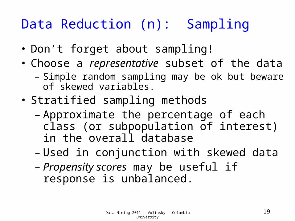
Data Reduction (n): Sampling
• Don’t forget about sampling!• Choose a representative subset of the data
– Simple random sampling may be ok but beware of skewed variables.
• Stratified sampling methods– Approximate the percentage of each
class (or subpopulation of interest) in the overall database
– Used in conjunction with skewed data– Propensity scores may be useful if
response is unbalanced.
19Data Mining 2011 - Volinsky - Columbia University
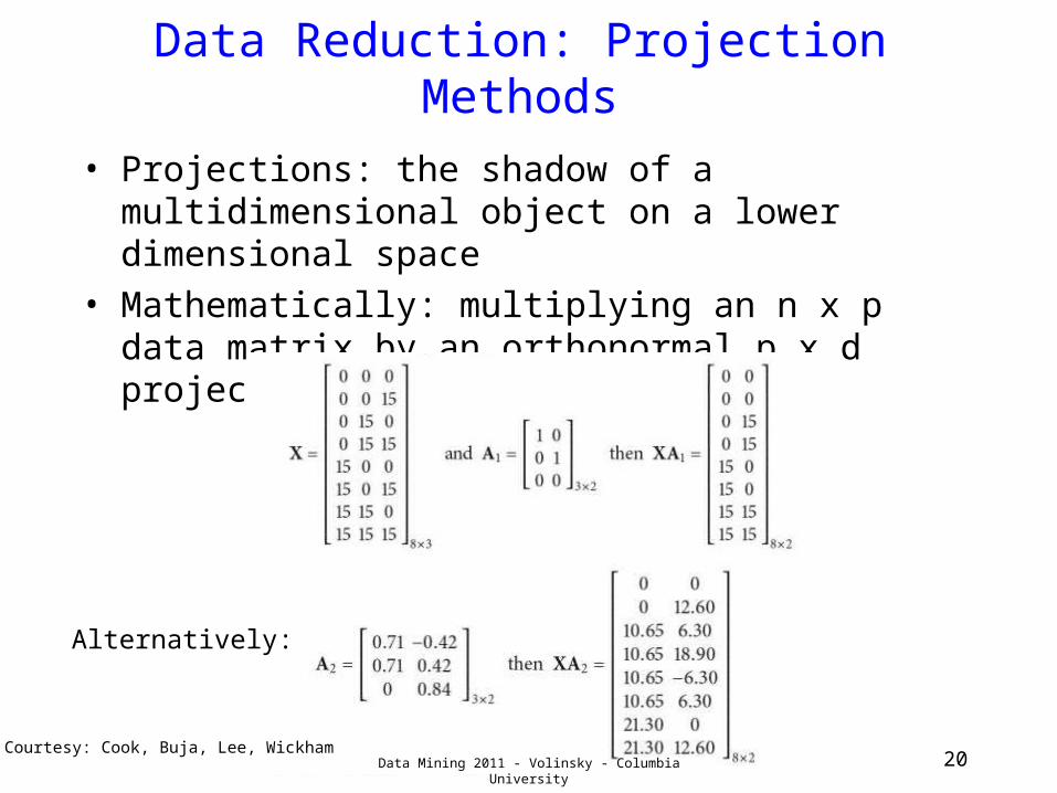
Data Reduction: Projection Methods
• Projections: the shadow of a multidimensional object on a lower dimensional space
• Mathematically: multiplying an n x p data matrix by an orthonormal p x d projection matrix
20
Alternatively:
Courtesy: Cook, Buja, Lee, WickhamData Mining 2011 - Volinsky - Columbia University

Projections
21Courtesy: Cook, Buja, Lee, Wickham Data Mining 2011 - Volinsky - Columbia University

Data Reduction: Principal Components
• One of several projection methods
• Idea: Find a projection of your data in a lower dimension, that maximizes the amount of information retained
• Information = variance
• Works for numeric data only
• Used when the number of dimensions is large
22Data Mining 2011 - Volinsky - Columbia University

PCA Example
23
Direction of 1st principal component vector (highest variance projection)
x1
x2
Data Mining 2011 - Volinsky - Columbia University

PCA Example
24
Direction of 1st principal component vector (highest variance projection)
x1
x2
Direction of 2ndprincipal component vector
Data Mining 2011 - Volinsky - Columbia University
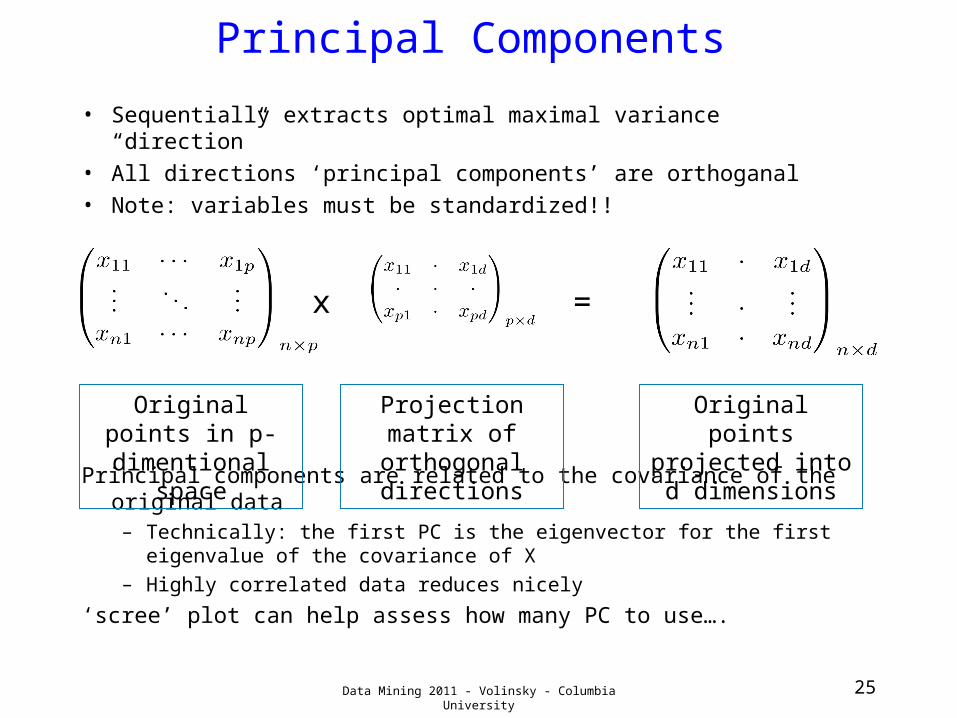
Principal Components
• Sequentially extracts optimal maximal variance “direction”• All directions ‘principal components’ are orthoganal• Note: variables must be standardized!!
Principal components are related to the covariance of the original data– Technically: the first PC is the eigenvector for the first
eigenvalue of the covariance of X– Highly correlated data reduces nicely
‘scree’ plot can help assess how many PC to use….
25Data Mining 2011 - Volinsky - Columbia University
x =
Original points in p-dimentional
space
Projection matrix of
orthogonal directions
Original points projected into d
dimensions
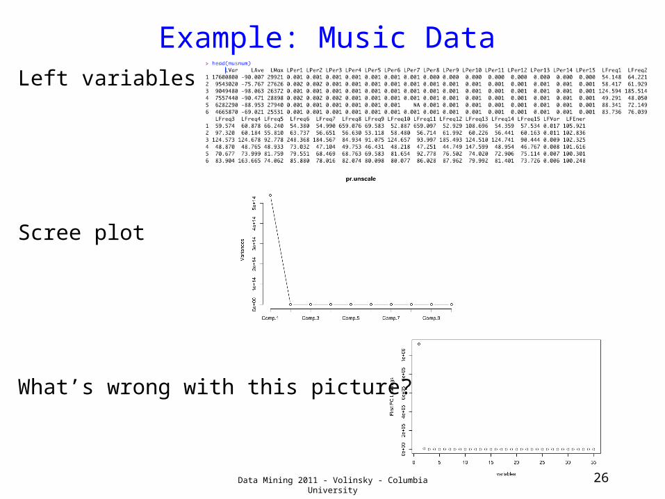
Example: Music DataLeft variables
Scree plot
What’s wrong with this picture?
Data Mining 2011 - Volinsky - Columbia University 26
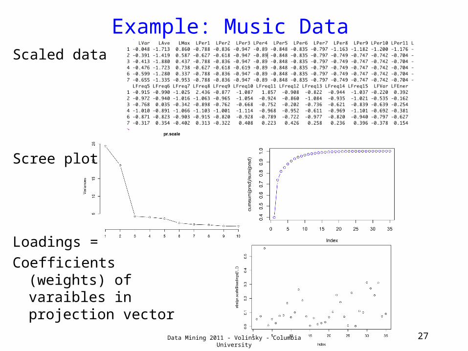
Example: Music DataScaled data
Scree plot
Loadings =Coefficients
(weights) of varaibles in projection vector Data Mining 2011 - Volinsky - Columbia University 27
Data Reduction: Multidimensional Scaling
• Start with an n x p matrix of observations and variables
• Create an n x n matrix of distances (similarities)– Feasible when n small(ish)– 0’s on the diagonal– Symmetric
• Or, you may have a distance of matrices to start with– Relationships, networks, etc
• MDS:– finds a representation of these points in a lower-dimensional
space usually 2), where the distances in this space best represent the original distances
28Data Mining 2011 - Volinsky - Columbia University
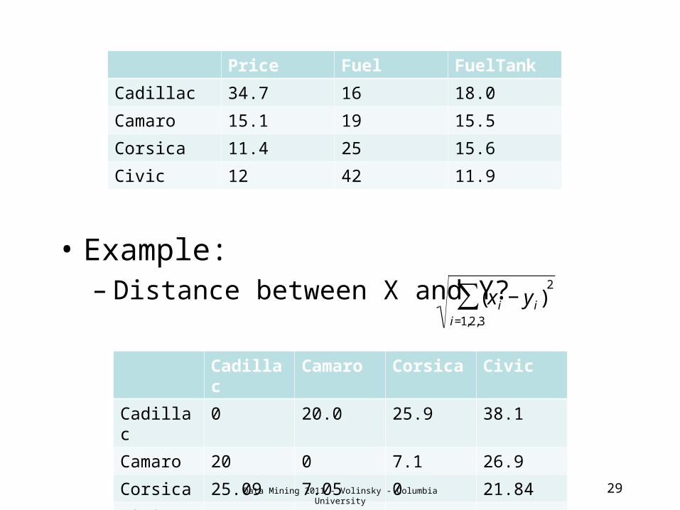
• Example:– Distance between X and Y?
29
Price Fuel FuelTank
Cadillac 34.7 16 18.0
Camaro 15.1 19 15.5
Corsica 11.4 25 15.6
Civic 12 42 11.9
€
(x i − y i)i=1,2,3
∑2
Cadillac Camaro Corsica Civic
Cadillac 0 20.0 25.9 38.1
Camaro 20 0 7.1 26.9
Corsica 25.09 7.05 0 21.84
Civic 38.1 26.9 21.84 0Data Mining 2011 - Volinsky - Columbia University
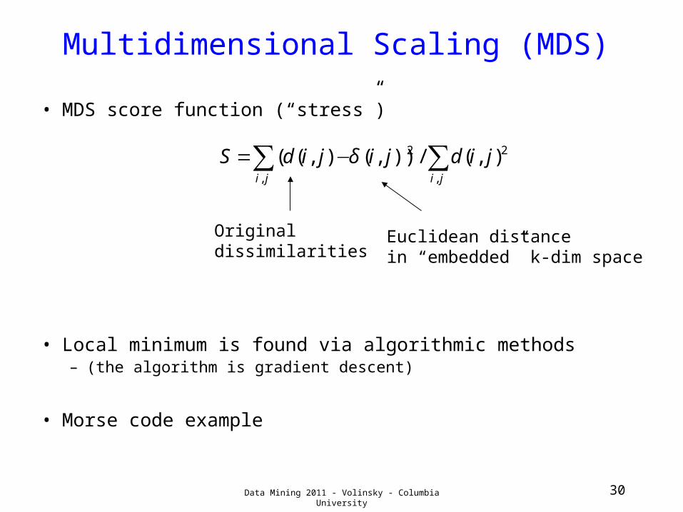
Multidimensional Scaling (MDS)
• MDS score function (“stress”)
• Local minimum is found via algorithmic methods– (the algorithm is gradient descent)
• Morse code example
∑∑ −=jiji
jidjijidS,
2
,
2 ),(/)),(),(( δ
30
Originaldissimilarities
Euclidean distancein “embedded” k-dim space
Data Mining 2011 - Volinsky - Columbia University

MDS: face data
31Data Mining 2011 - Volinsky - Columbia University

MDS: 2d embedding of face images
32Data Mining 2011 - Volinsky - Columbia University
Similar faces are close to each other
Sometimes the axes can have an interpretation

Data Mining 2011 - Volinsky - Columbia University 33
Model Evaluation
34Data Mining 2011 - Volinsky - Columbia University
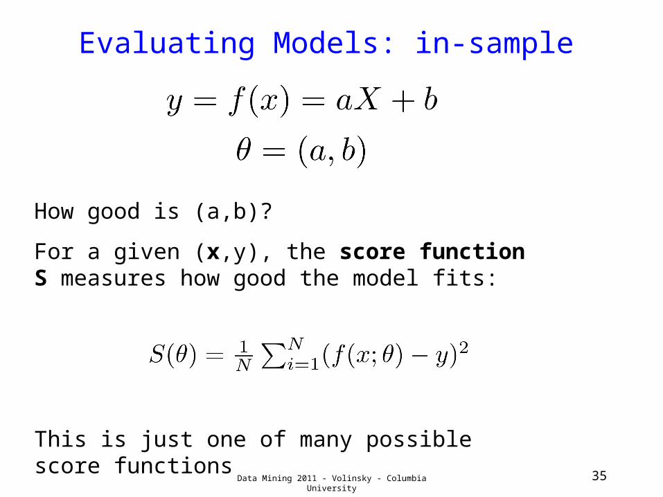
Evaluating Models: in-sample
35
How good is (a,b)?
For a given (x,y), the score function S measures how good the model fits:
This is just one of many possible score functions
Data Mining 2011 - Volinsky - Columbia University
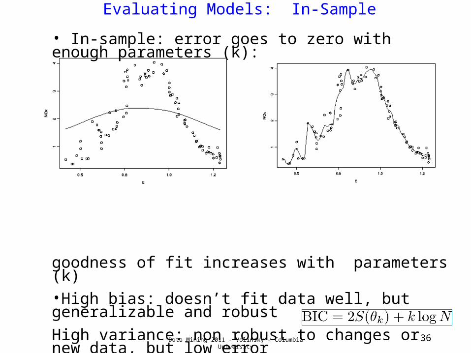
Evaluating Models: In-Sample
36
• In-sample: error goes to zero with enough parameters (k):
goodness of fit increases with parameters (k)•High bias: doesn’t fit data well, but generalizable and robust
High variance: non robust to changes or new data, but low error
Score function should embody the comprimise:
score(model) = Goodness-of-fit - penalty(k)
e.g. Bayesian Information Criterion
Data Mining 2011 - Volinsky - Columbia University

In v. Out
• In-sample evaluation– Uses all of the data to fit parameters– Focus: how well does my model ‘fit’ the data– Penalties to decide on number of parameters
• Out-of-sample evaluation– Split data into training and test sets– Focus: how well does my model predict things– Prediction error is all that matters
• Statistics traditionally looks at in-sample where as data mining / machine learning typically uses out-of-sample
37Data Mining 2011 - Volinsky - Columbia University
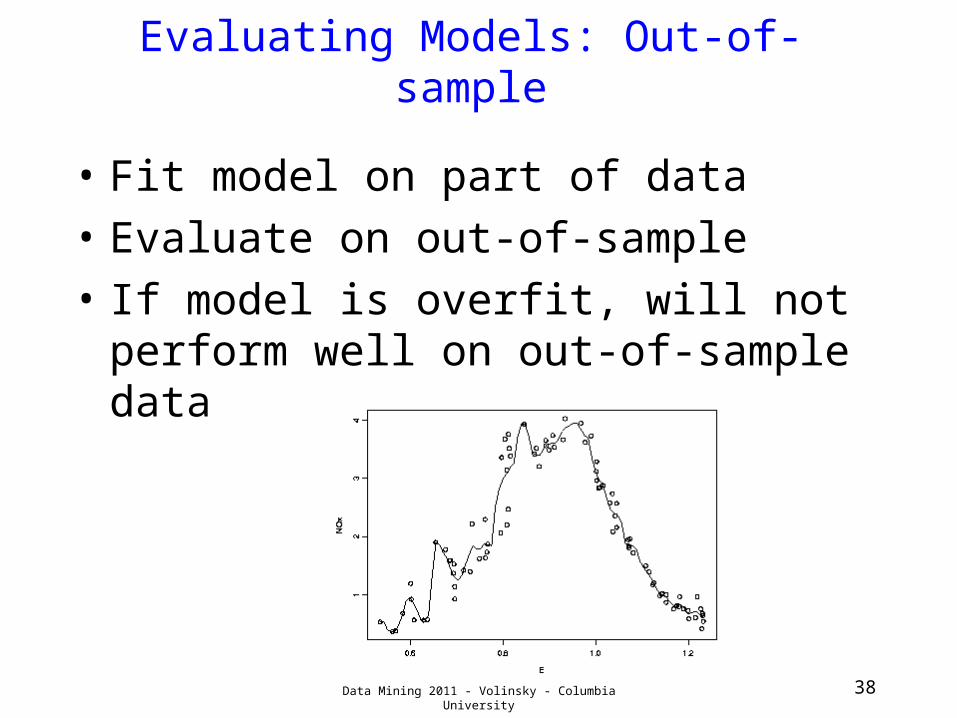
Evaluating Models: Out-of-sample
• Fit model on part of data• Evaluate on out-of-sample• If model is overfit, will not perform
well on out-of-sample data
38Data Mining 2011 - Volinsky - Columbia University

Data Partitioning
• Randomly partition data into training and test set• Training set – data used to train/build the model.
– Estimate parameters (e.g., for a linear regression), build decision tree, build artificial network, etc.
• Test set – a set of examples not used for model induction. The model’s performance is evaluated on unseen data. Aka out-of-sample data.
• Generalization Error: Model error on the test data.
39
Set of training examplesSet of testexamples
Data Mining 2011 - Volinsky - Columbia University
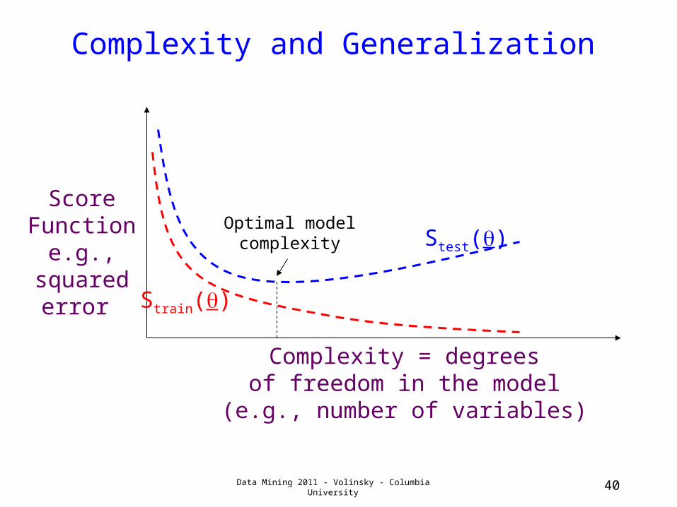
Data Mining 2011 - Volinsky - Columbia University
Complexity and Generalization
Strain()
Stest()
Complexity = degreesof freedom in the model
(e.g., number of variables)
Score Function
e.g., squarederror
Optimal modelcomplexity
40

Holding out data
• The holdout method reserves a certain amount for testing and uses the remainder for training– Usually: one third for testing, the rest for
training
• For “unbalanced” datasets, random samples might not be representative– Few or none instances of some classes
• Stratified sample: – Make sure that each class is represented with
approximately equal proportions in both subsets
4141 Data Mining 2011 - Volinsky - Columbia University
Repeated holdout method
• Holdout estimate can be made more reliable by repeating the process with different subsamples– In each iteration, a certain proportion is
randomly selected for training (possibly with stratification)
– The error rates on the different iterations are averaged to yield an overall error rate
• This is called the repeated holdout method
4242 Data Mining 2011 - Volinsky - Columbia University
Cross-validation
• Most popular and effective type of repeated holdout is cross-validation
• Cross-validation avoids overlapping test sets– First step: data is split into k subsets of
equal size– Second step: each subset in turn is used for
testing and the remainder for training
• This is called k-fold cross-validation• Often the subsets are stratified before
the cross-validation is performed
4343 Data Mining 2011 - Volinsky - Columbia University
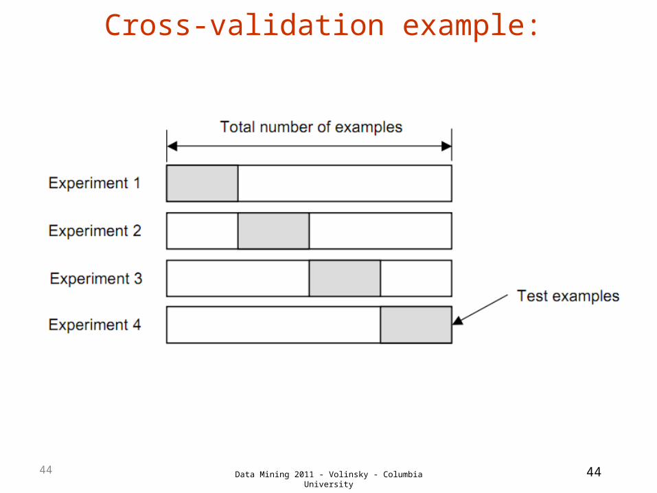
Cross-validation example:
Data Mining 2011 - Volinsky - Columbia University 4444 44

More on cross-validation
• Standard data-mining method for evaluation: stratified ten-fold cross-validation
• Why ten? Extensive experiments have shown that this is the best choice to get an accurate estimate
• Stratification reduces the estimate’s variance• Even better: repeated stratified cross-validation
– E.g. ten-fold cross-validation is repeated ten times and results are averaged (reduces the sampling variance)
• Error estimate is the mean across all repetitions
4545 Data Mining 2011 - Volinsky - Columbia University
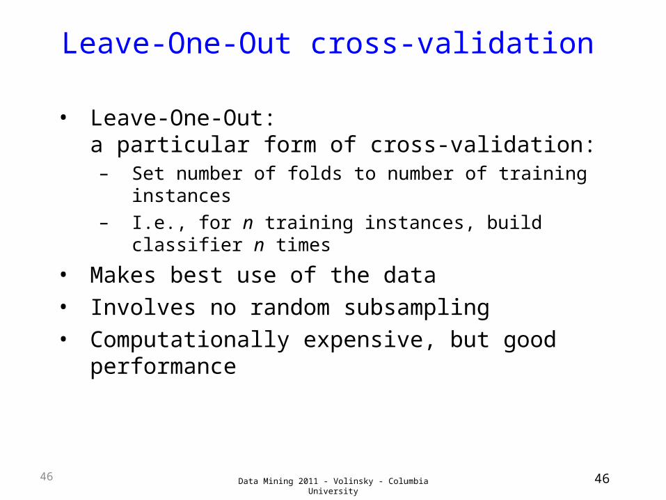
Leave-One-Out cross-validation
• Leave-One-Out:a particular form of cross-validation:– Set number of folds to number of training
instances– I.e., for n training instances, build classifier n
times
• Makes best use of the data• Involves no random subsampling • Computationally expensive, but good
performance
4646 Data Mining 2011 - Volinsky - Columbia University

Leave-One-Out-CV and stratification
• Disadvantage of Leave-One-Out-CV: stratification is not possible– It guarantees a non-stratified sample because
there is only one instance in the test set!
• Extreme example: random dataset split equally into two classes– Best model predicts majority class– 50% accuracy on fresh data – Leave-One-Out-CV estimate is 100% error!
4747 Data Mining 2011 - Volinsky - Columbia University

Three way data splits
• One problem with CV is since data is being used jointly to fit model and estimate error, the error could be biased downward.
• If the goal is a real estimate of error (as opposed to which model is best), you may want a three way split:– Training set: examples used for learning– Validation set: used to tune parameters– Test set: never used in the model fitting
process, used at the end for unbiased estimate of hold out error
Data Mining 2011 - Volinsky - Columbia University 48
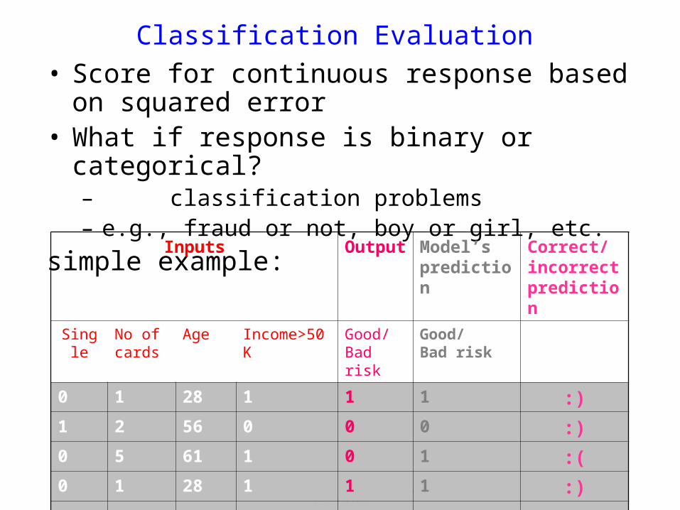
Classification Evaluation• Score for continuous response based on
squared error• What if response is binary or categorical?
– classification problems– e.g., fraud or not, boy or girl, etc.
simple example:
49Data Mining 2011 - Volinsky - Columbia University
Inputs Output Model’s prediction
Correct/incorrect prediction
Single No of cards
Age Income>50K Good/Bad risk
Good/Bad risk
0 1 28 1 1 1 :)
1 2 56 0 0 0 :)
0 5 61 1 0 1 :(
0 1 28 1 1 1 :)
… … … … … … …
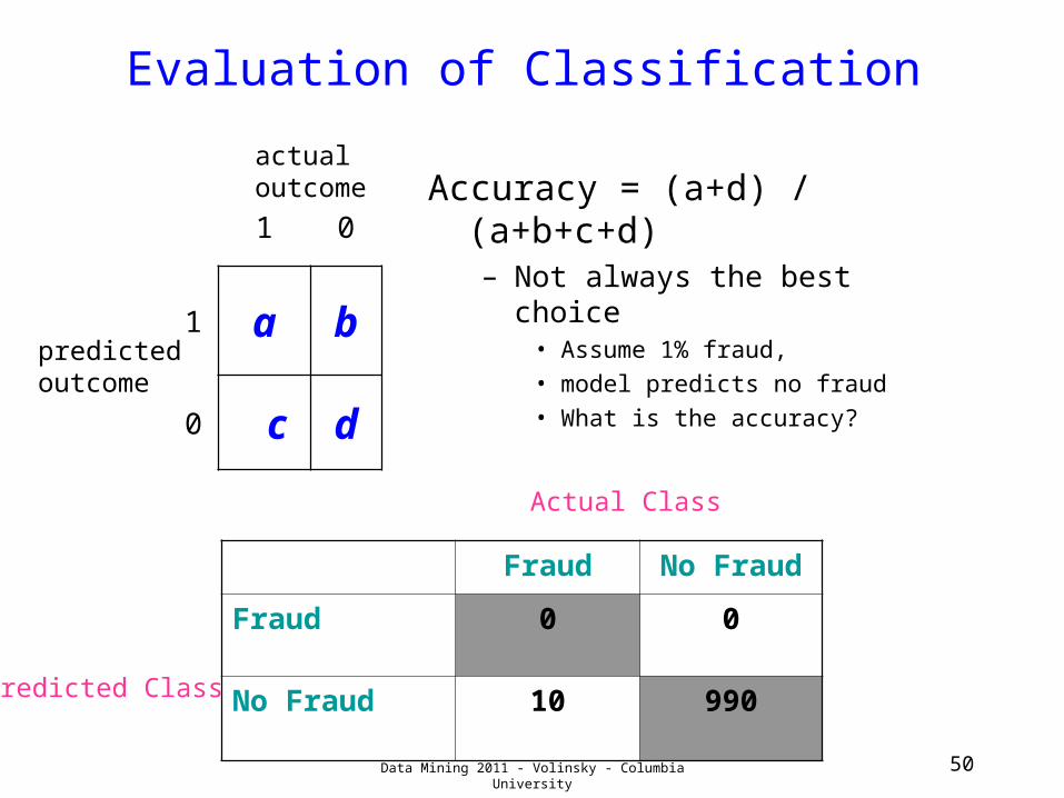
Evaluation of Classification
Accuracy = (a+d) / (a+b+c+d)– Not always the best choice
• Assume 1% fraud, • model predicts no fraud• What is the accuracy?
Data Mining 2011 - Volinsky - Columbia University 50
1 0
1 a b
0 c d
predictedoutcome
actualoutcome
Fraud No Fraud
Fraud 0 0
No Fraud 10 990Predicted Class
Actual Class

Evaluation of Classification
Other options:– recall or sensitivity (how many of those that are
really positive did you predict?):• a/(a+c)
– precision (how many of those predicted positive really are?)
• a/(a+b)
Precision and recall are always in tension– Increasing one tends to decrease another– Document retrieval example
Data Mining 2011 - Volinsky - Columbia University 51
1 0
1 a b
0 c d
predictedoutcome
actualoutcome
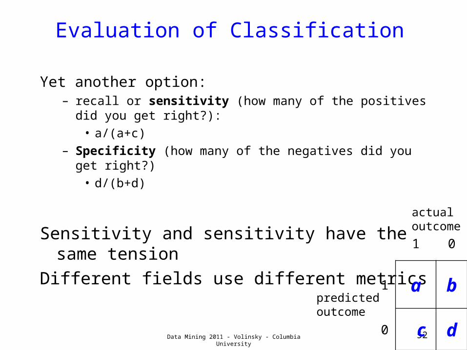
Evaluation of Classification
Yet another option:– recall or sensitivity (how many of the positives did
you get right?):• a/(a+c)
– Specificity (how many of the negatives did you get right?)
• d/(b+d)
Sensitivity and sensitivity have the same tension
Different fields use different metrics
Data Mining 2011 - Volinsky - Columbia University 52
1 0
1 a b
0 c d
predictedoutcome
actualoutcome
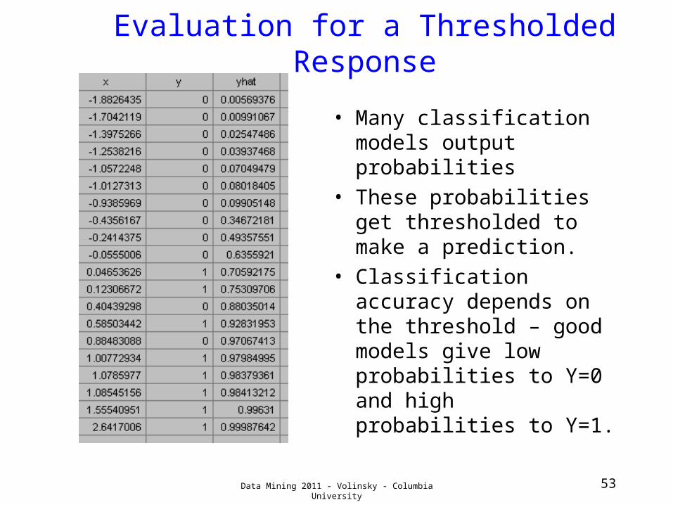
Evaluation for a Thresholded Response
• Many classification models output probabilities
• These probabilities get thresholded to make a prediction.
• Classification accuracy depends on the threshold – good models give low probabilities to Y=0 and high probabilities to Y=1.
53Data Mining 2011 - Volinsky - Columbia University
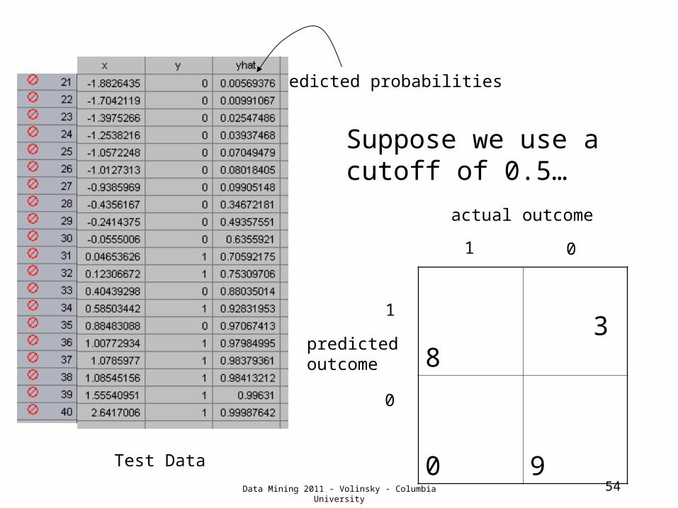
54
Test Data
predicted probabilities
8 3
0 9
1
0
01
actual outcome
predictedoutcome
Suppose we use a cutoff of 0.5…
Data Mining 2011 - Volinsky - Columbia University

55
8 3
0 9
1
0
01
actual outcome
predictedoutcome
Suppose we use a cutoff of 0.5…
sensitivity: = 100% 8
8+0
specificity: = 75% 9
9+3
we want both of these to be high
Data Mining 2011 - Volinsky - Columbia University

56
6 2
2 10
1
0
01
actual outcome
predictedoutcome
Suppose we use a cutoff of 0.8…
sensitivity: = 75% 6
6+2
specificity: = 83% 10
10+2
Data Mining 2011 - Volinsky - Columbia University
57
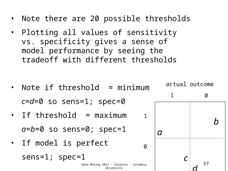
• Note there are 20 possible thresholds
• Plotting all values of sensitivity vs. specificity gives a sense of model performance by seeing the tradeoff with different thresholds
• Note if threshold = minimum
c=d=0 so sens=1; spec=0
• If threshold = maximum
a=b=0 so sens=0; spec=1
• If model is perfect
sens=1; spec=1
a b
c d
1
0
01
actual outcome
Data Mining 2011 - Volinsky - Columbia University
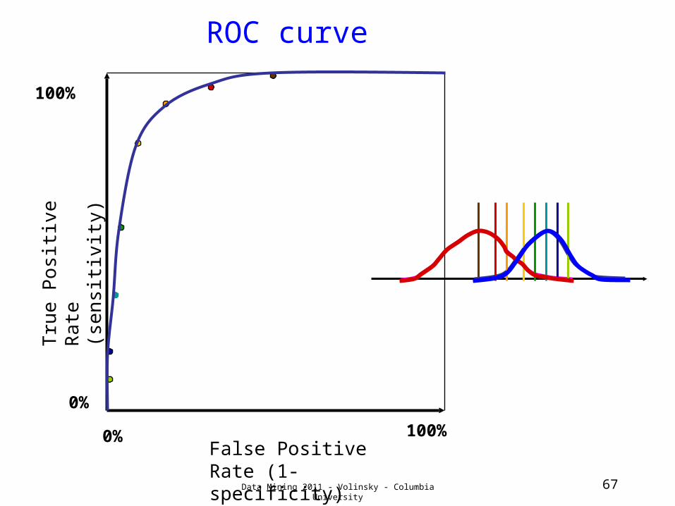
58Data Mining 2011 - Volinsky - Columbia University
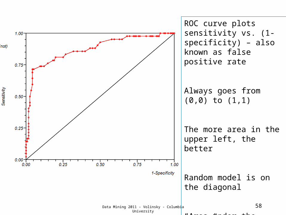
ROC curve plots sensitivity vs. (1-specificity) – also known as false positive rate
Always goes from (0,0) to (1,1)
The more area in the upper left, the better
Random model is on the diagonal
“Area under the curve” (AUC) is a common measure of predictive performance

59
Another Look at ROC Curves
Test Result
Pts Pts with with diseasdiseasee
Pts Pts without without the the diseasedisease
Data Mining 2011 - Volinsky - Columbia University

60
Threshold
Test Result
Call these patients “negative”
Call these patients “positive”
Data Mining 2011 - Volinsky - Columbia University

61
Some definitions ...
Test Result
Call these patients “negative”
Call these patients “positive”
without the diseasewith the disease
True Positives
Data Mining 2011 - Volinsky - Columbia University
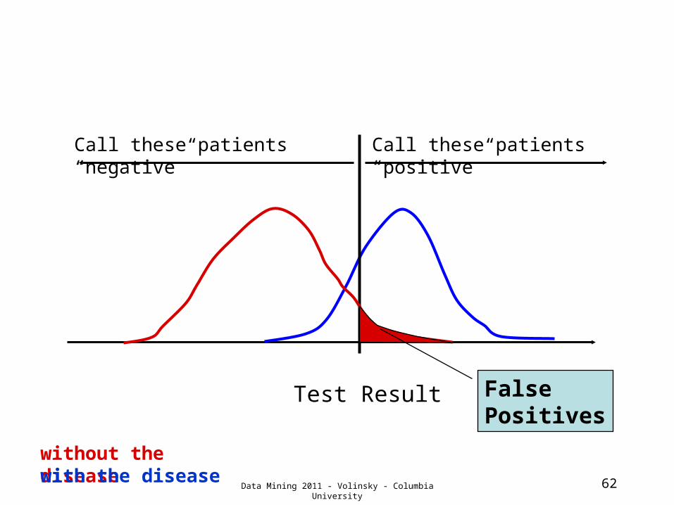
62
Test Result
Call these patients “negative”
Call these patients “positive”
without the diseasewith the disease
False Positives
Data Mining 2011 - Volinsky - Columbia University

63
Test Result
Call these patients “negative”
Call these patients “positive”
without the diseasewith the disease
True negatives
Data Mining 2011 - Volinsky - Columbia University
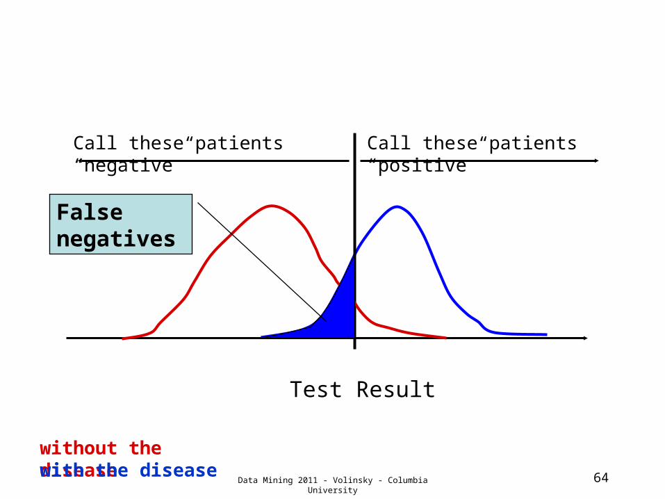
64
Test Result
Call these patients “negative”
Call these patients “positive”
without the diseasewith the disease
False negatives
Data Mining 2011 - Volinsky - Columbia University
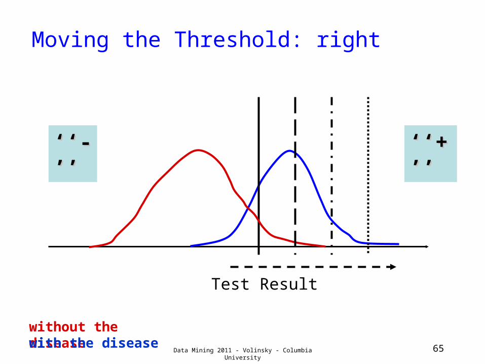
65
Moving the Threshold: right
Test Result
without the diseasewith the disease
‘‘‘‘-’-’’’
‘‘‘‘+’+’’’
Data Mining 2011 - Volinsky - Columbia University
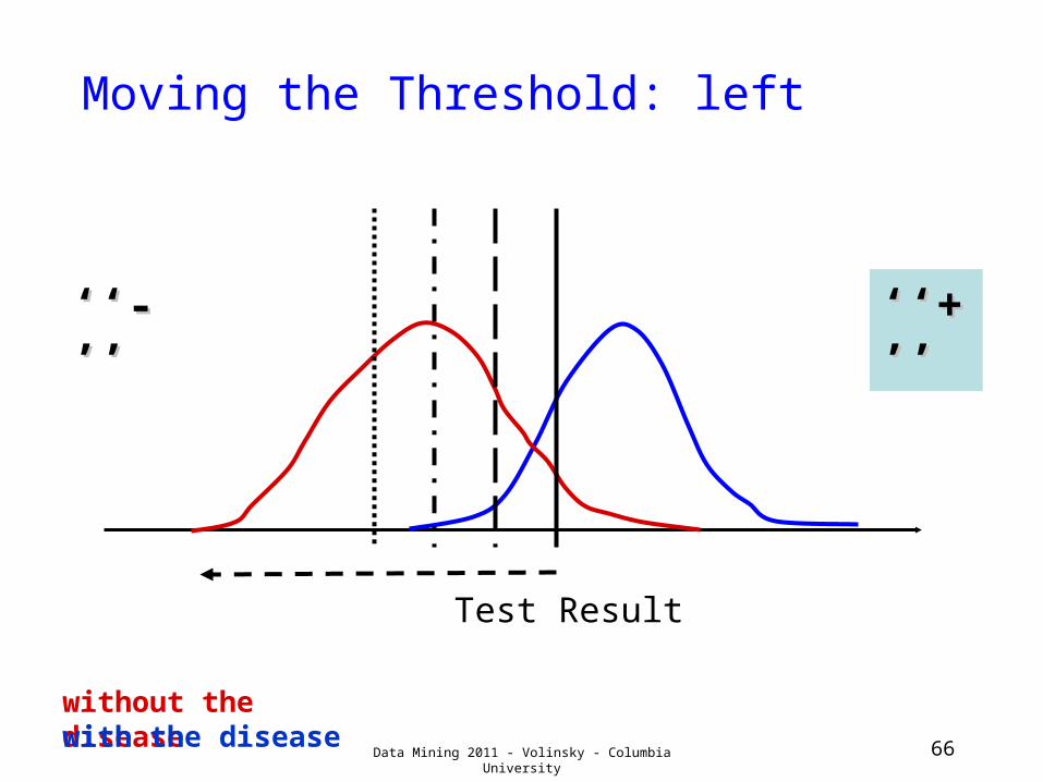
66
Moving the Threshold: left
Test Result
without the diseasewith the disease
‘‘‘‘-’-’’’
‘‘‘‘+’+’’’
Data Mining 2011 - Volinsky - Columbia University
67
ROC curveTru
e P
osi
tive R
ate
(s
en
siti
vit
y)
0%
100%
False Positive Rate (1-specificity)
0%
100%
Data Mining 2011 - Volinsky - Columbia University
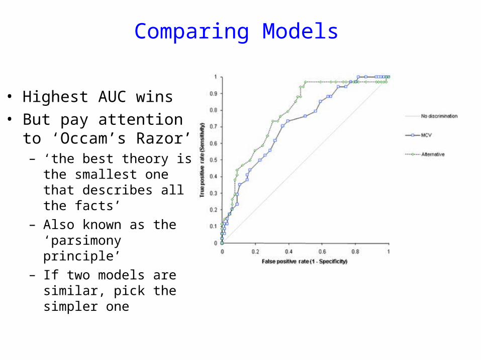
Comparing Models
• Highest AUC wins• But pay attention to
‘Occam’s Razor’– ‘the best theory is the
smallest one that describes all the facts’
– Also known as the ‘parsimony principle’
– If two models are similar, pick the simpler one

Incorporating cost functions
• Not all errors are the same:– Loan payments
• A bad loan costs us much more than a lost customer
– Medical tests• Cost of false alarm vs. missed diagnosis
– Spam• Cost of spam getting through vs. filtering
important mail
• Building algorithm to minimize cost is the same as adding weight to false neg and false pos
Data Mining 2011 - Volinsky - Columbia University 6969
1 0
1 0C(FP)
0 C(FN)
0
predictedoutcome
actualoutcome