Chapter 3 Bernoulli Equation - User page server for...
26
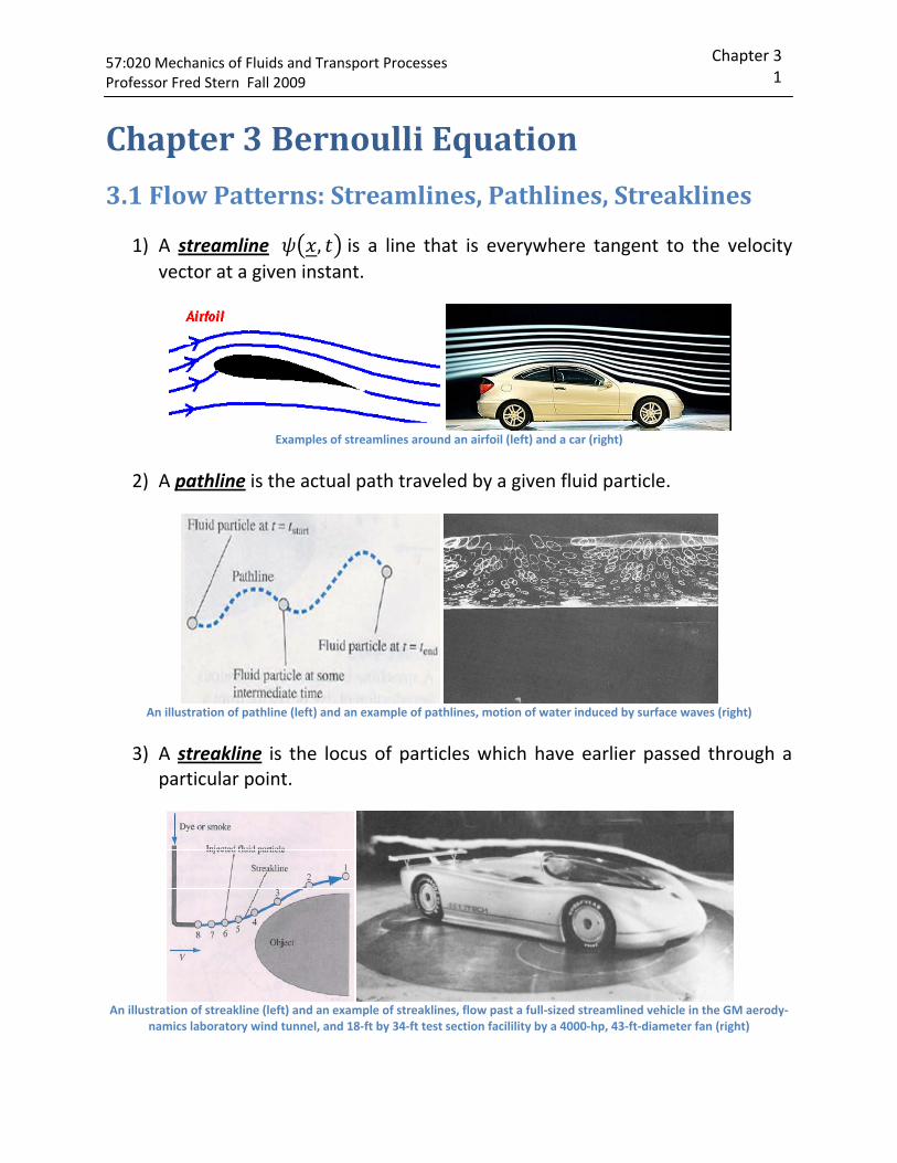
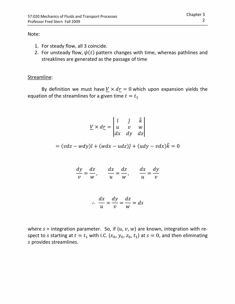
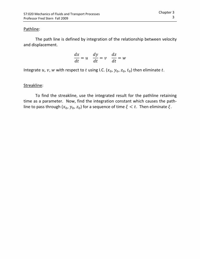
57:020 Mechanics of Fluids and Transport Processes Professor Fred Stern Fall 2009 Chapter 3 1 Chapter 3 Bernoulli Equation 3.1 Flow Patterns: Streamlines, Pathlines, Streaklines 1) A streamline ൫ ݔݐ,൯ is a line that is everywhere tangent to the velocity vector at a given instant. Examples of streamlines around an airfoil (left) and a car (right) 2) A pathline is the actual path traveled by a given fluid particle. An illustration of pathline (left) and an example of pathlines, motion of water induced by surface waves (right) 3) A streakline is the locus of particles which have earlier passed through a particular point. An illustration of streakline (left) and an example of streaklines, flow past a full-sized streamlined vehicle in the GM aerody- namics laboratory wind tunnel, and 18-ft by 34-ft test section facilility by a 4000-hp, 43-ft-diameter fan (right)
Transcript of Chapter 3 Bernoulli Equation - User page server for...
57:020 Mechanics of Fluids and Transport Processes Professor Fred Stern Fall 2009
Chapter 3 1
Chapter 3 Bernoulli Equation
3.1 Flow Patterns: Streamlines, Pathlines, Streaklines
1) A streamline , is a line that is everywhere tangent to the velocity vector at a given instant.
Examples of streamlines around an airfoil (left) and a car (right)
2) A pathline is the actual path traveled by a given fluid particle.
An illustration of pathline (left) and an example of pathlines, motion of water induced by surface waves (right)
3) A streakline is the locus of particles which have earlier passed through a particular point.
An illustration of streakline (left) and an example of streaklines, flow past a full-sized streamlined vehicle in the GM aerody-
namics laboratory wind tunnel, and 18-ft by 34-ft test section facilility by a 4000-hp, 43-ft-diameter fan (right)
57:020 Mechanics of Fluids and Transport Processes Professor Fred Stern Fall 2009
Chapter 3 2
Note:
1. For steady flow, all 3 coincide. 2. For unsteady flow, pattern changes with time, whereas pathlines and
streaklines are generated as the passage of time
Streamline:
By definition we must have 0 which upon expansion yields the equation of the streamlines for a given time
0
, ,
where = integration parameter. So, if ( , , ) are known, integration with re-spect to starting at with I.C. ( , , , ) at 0, and then eliminating
provides streamlines.
57:020 Mechanics of Fluids and Transport Processes Professor Fred Stern Fall 2009
Chapter 3 3
Pathline:
The path line is defined by integration of the relationship between velocity and displacement.
Integrate , , with respect to using I.C. ( , , , ) then eliminate .
Streakline:
To find the streakline, use the integrated result for the pathline retaining time as a parameter. Now, find the integration constant which causes the path-line to pass through ( , , ) for a sequence of time . Then eliminate .
57:020 Mechanics of Fluids and Transport Processes Professor Fred Stern Fall 2009
Chapter 3 4
3.2 Streamline Coordinates
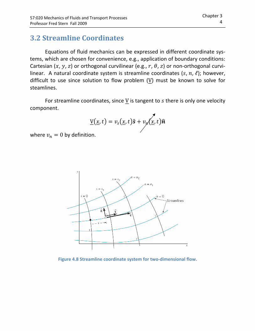
Equations of fluid mechanics can be expressed in different coordinate sys-tems, which are chosen for convenience, e.g., application of boundary conditions: Cartesian ( , , ) or orthogonal curvilinear (e.g., , , ) or non-orthogonal curvi-linear. A natural coordinate system is streamline coordinates ( , , ℓ); however, difficult to use since solution to flow problem (V) must be known to solve for steamlines.
For streamline coordinates, since V is tangent to there is only one velocity component. V , , ,
where 0 by definition.
Figure 4.8 Streamline coordinate system for two-dimensional flow.
57:020 Mechanics of Fluids and Transport Processes Professor Fred Stern Fall 2009
Chapter 3 5
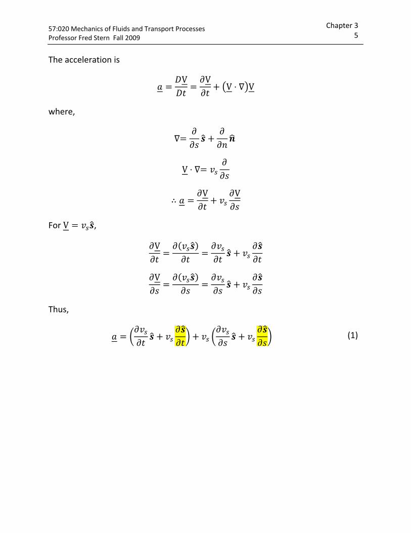
The acceleration is V V V V
where,
V V V
For V , V V
Thus,
(1)
57:020 Mechanics of Fluids and Transport Processes Professor Fred Stern Fall 2009
Chapter 3 6
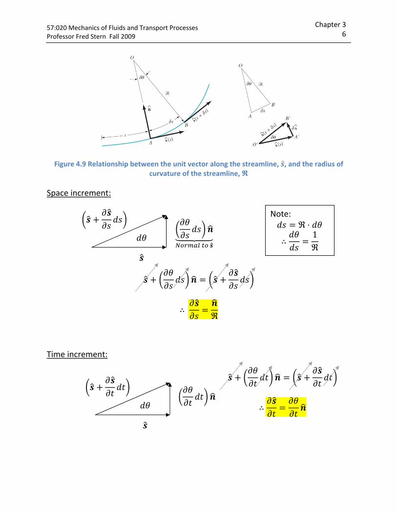
Figure 4.9 Relationship between the unit vector along the streamline, , and the radius of curvature of the streamline,
Space increment:
Time increment:
1
Note:
57:020 Mechanics of Fluids and Transport Processes Professor Fred Stern Fall 2009
Chapter 3 7
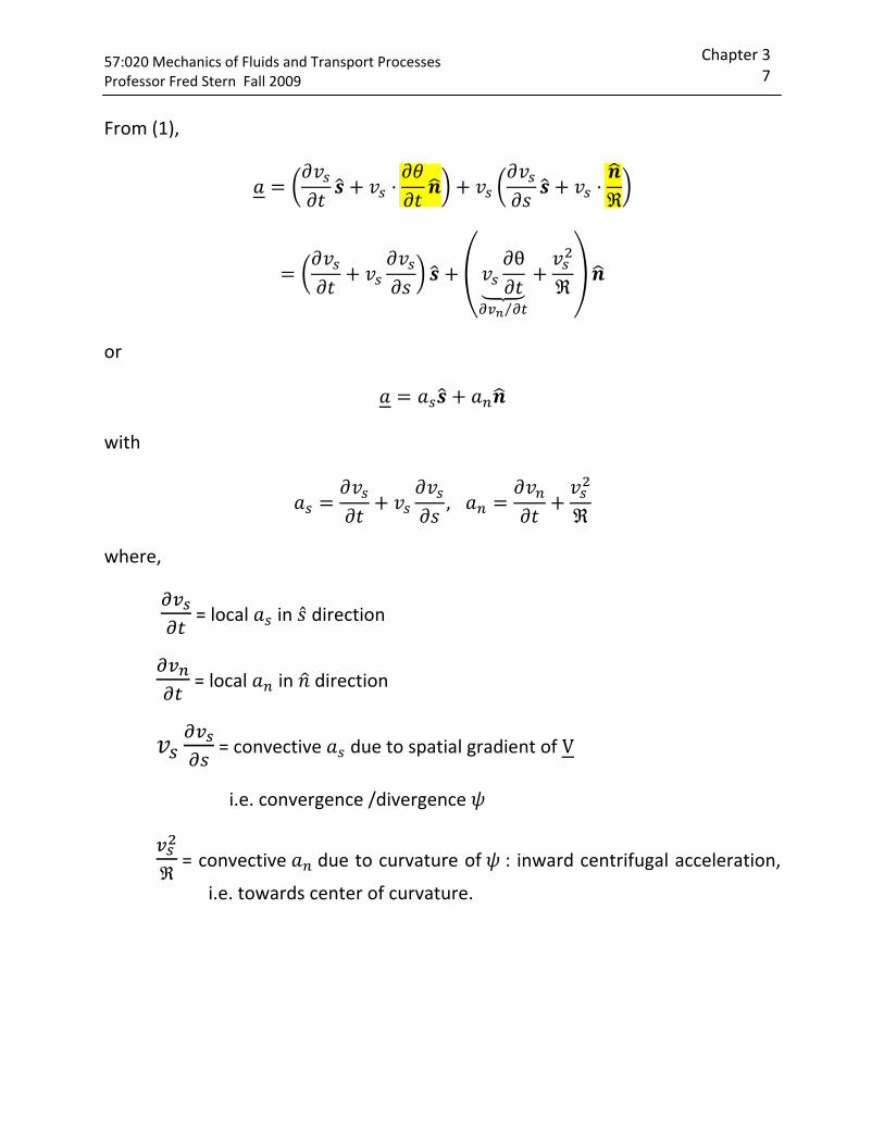
From (1),
θ⁄
or
with
,
where,
= local in direction
= local in direction
= convective due to spatial gradient of V
i.e. convergence /divergence
= convective due to curvature of : inward centrifugal acceleration,
i.e. towards center of curvature.
57:020 Mechanics of Fluids and Transport Processes Professor Fred Stern Fall 2009
Chapter 3 8
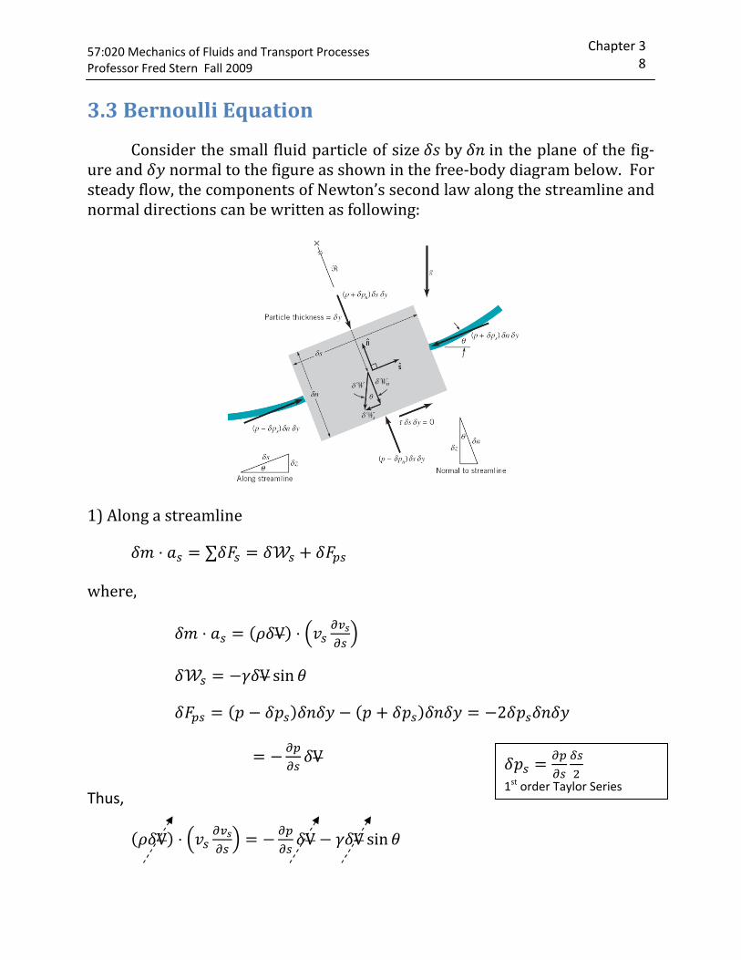
3.3 Bernoulli Equation Consider the small fluid particle of size by in the plane of the fig-ure and normal to the figure as shown in the free-body diagram below. For steady flow, the components of Newton’s second law along the streamline and normal directions can be written as following:
1) Along a streamline ∑ where, V V sin
2
V
Thus,
V V V sin
1st order Taylor Series
57:020 Mechanics of Fluids and Transport Processes Professor Fred Stern Fall 2009
Chapter 3 9
sin
→ change in speed due to and (i.e. along )
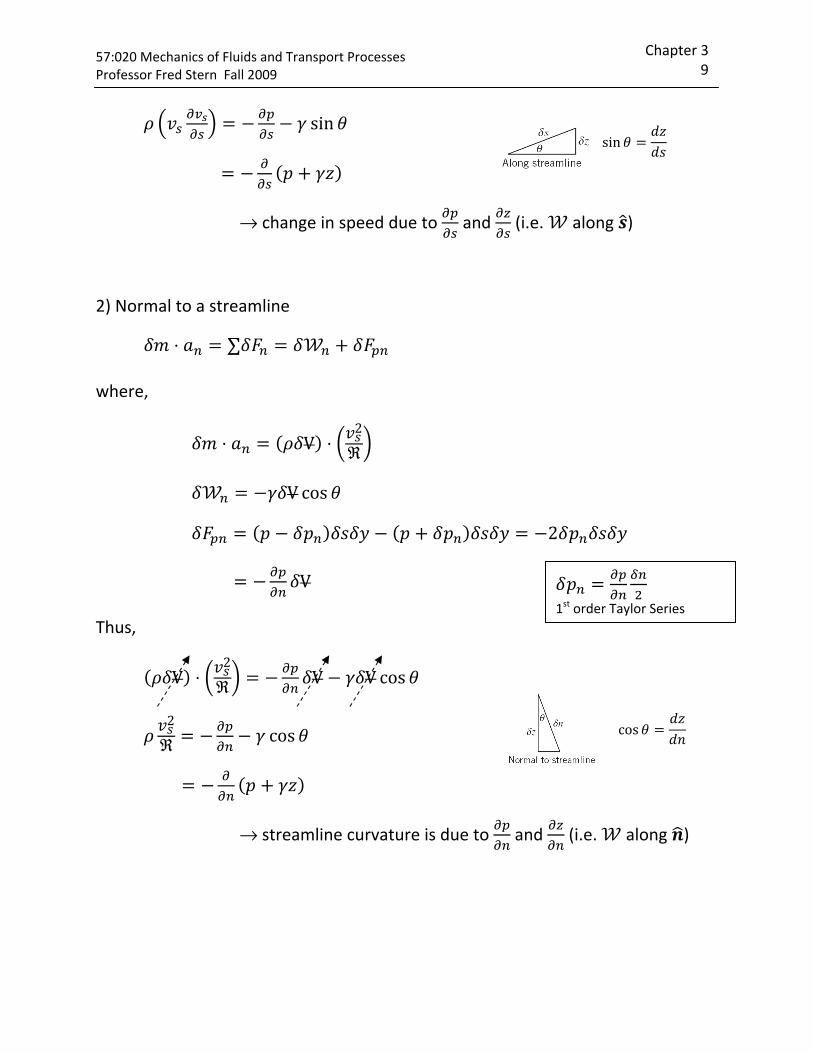
2) Normal to a streamline
∑
where,
V 2
V cos
2
V
Thus,
V 2 V V cos
2 cos
→ streamline curvature is due to and (i.e. along )
1st order Taylor Series
sin
cos
57:020 Mechanics of Fluids and Transport Processes Professor Fred Stern Fall 2009
Chapter 3 10
In a vector form:
(Euler equation)
or
Steady flow, = constant, equation
0
2
Steady flow, = constant, equation
For curved streamlines (= constant for static fluid) decreases in the di-rection, i.e. towards the local center of curvature.
It should be emphasized that the Bernoulli equation is restricted to the fol-lowing:
• inviscid flow • steady flow • incompressible flow • flow along a streamline
Note that if in addition to the flow being inviscid it is also irrotational, i.e. rotation of fluid = = vorticity = V = 0, the Bernoulli constant is same for all , as will be shown later.
57:020 Mechanics of Fluids and Transport Processes Professor Fred Stern Fall 2009
Chapter 3 11
3.4 Physical interpretation of Bernoulli equation
Integration of the equation of motion to give the Bernoulli equation actual-ly corresponds to the work-energy principle often used in the study of dynamics. This principle results from a general integration of the equations of motion for an object in a very similar to that done for the fluid particle. With certain assump-tions, a statement of the work-energy principle may be written as follows:
The work done on a particle by all forces acting on the particle is equal to the change of the kinetic energy of the particle.
The Bernoulli equation is a mathematical statement of this principle.
In fact, an alternate method of deriving the Bernoulli equation is to use the first and second laws of thermodynamics (the energy and entropy equations), ra-ther than Newton’s second law. With the approach restrictions, the general energy equation reduces to the Bernoulli equation.
An alternate but equivalent form of the Bernoulli equation is
2
along a streamline.
Pressure head:
Velocity head:
Elevation head:
The Bernoulli equation states that the sum of the pressure head, the velocity head, and the elevation head is constant along a streamline.
57:020 Mechanics of Fluids and Transport Processes Professor Fred Stern Fall 2009
Chapter 3 12
3.5 Static, Stagnation, Dynamic, and Total Pressure 12
along a streamline.
Static pressure:
Dynamic pressure:
Hydrostatic pressure:
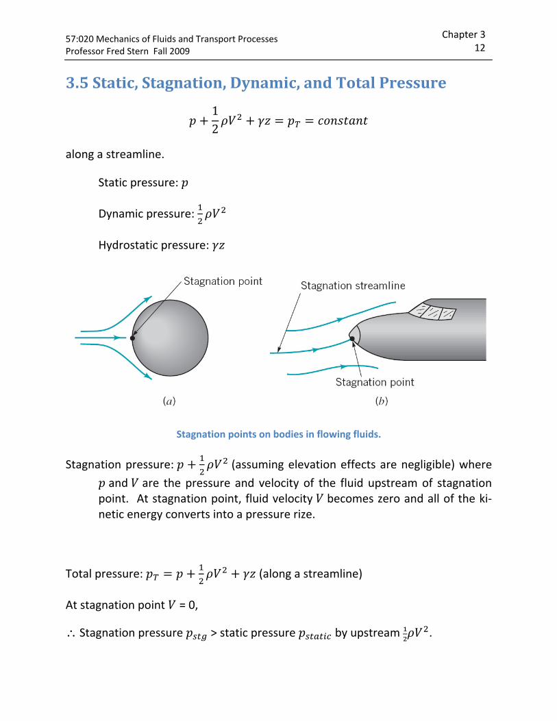
Stagnation points on bodies in flowing fluids.
Stagnation pressure: (assuming elevation effects are negligible) where
and are the pressure and velocity of the fluid upstream of stagnation point. At stagnation point, fluid velocity becomes zero and all of the ki-netic energy converts into a pressure rize.
Total pressure: (along a streamline)
At stagnation point = 0,
∴ Stagnation pressure > static pressure by upstream .
57:020 Mechanics of Fluids and Transport Processes Professor Fred Stern Fall 2009
Chapter 3 13
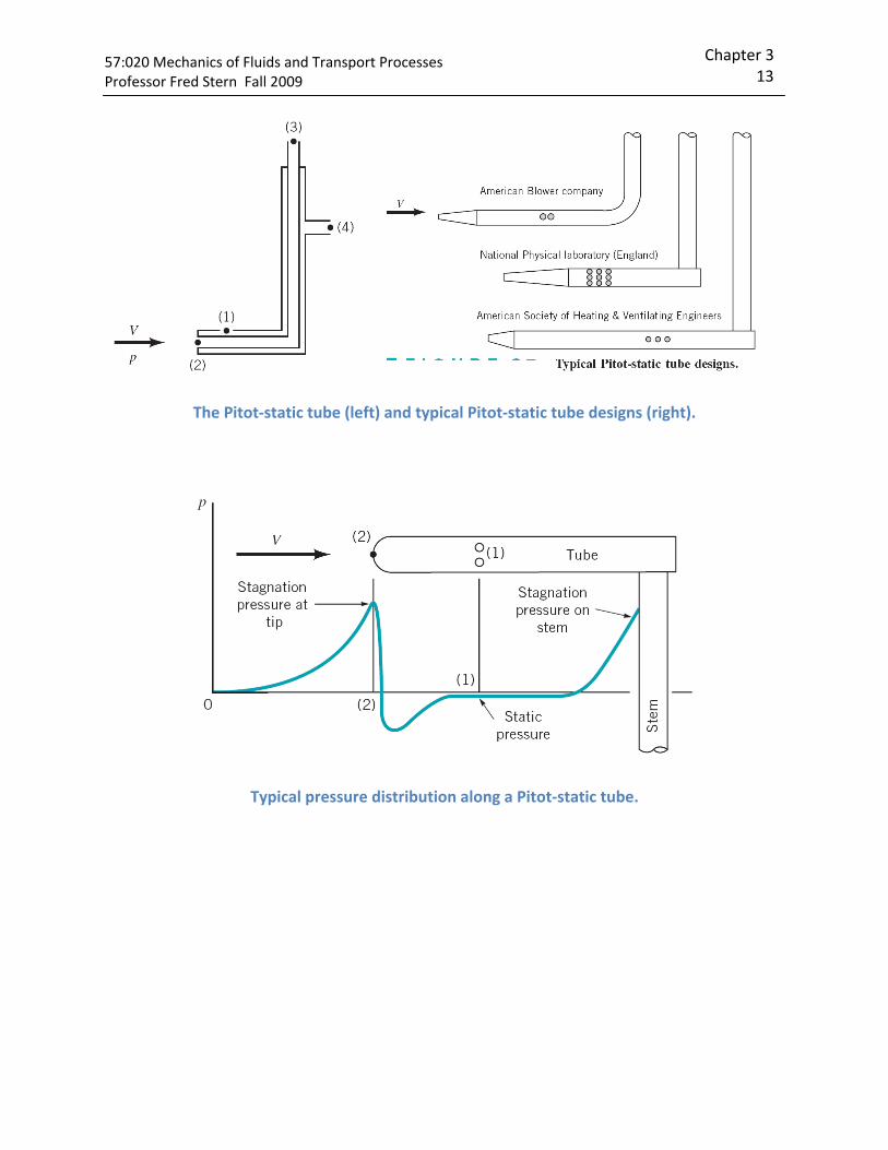
The Pitot-static tube (left) and typical Pitot-static tube designs (right).
Typical pressure distribution along a Pitot-static tube.
57:020 Mechanics of Fluids and Transport Processes Professor Fred Stern Fall 2009
Chapter 3 14
3.6 Applications of Bernoulli Equation
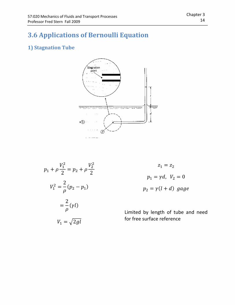
1) Stagnation Tube
2 2 2 2
2
, 0
Limited by length of tube and need for free surface reference
57:020 Mechanics of Fluids and Transport Processes Professor Fred Stern Fall 2009
Chapter 3 15
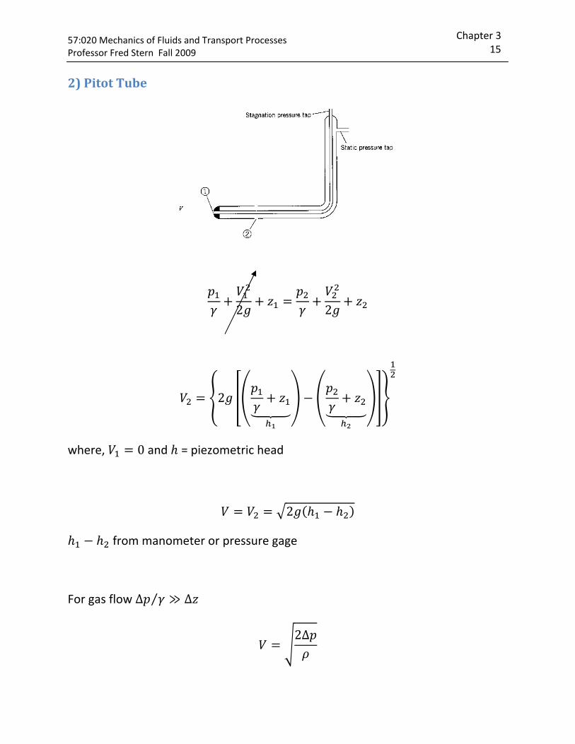
2) Pitot Tube
2 2
2
where, 0 and = piezometric head
2
from manometer or pressure gage
For gas flow Δ ⁄ Δ 2Δ
57:020 Mechanics of Fluids and Transport Processes Professor Fred Stern Fall 2009
Chapter 3 16
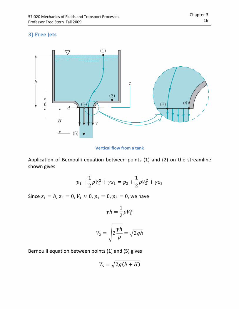
3) Free Jets
Vertical flow from a tank
Application of Bernoulli equation between points (1) and (2) on the streamline shown gives 12 12
Since , 0, 0, 0, 0, we have 12
2 2
Bernoulli equation between points (1) and (5) gives 2
57:020 Mechanics of Fluids and Transport Processes Professor Fred Stern Fall 2009
Chapter 3 17
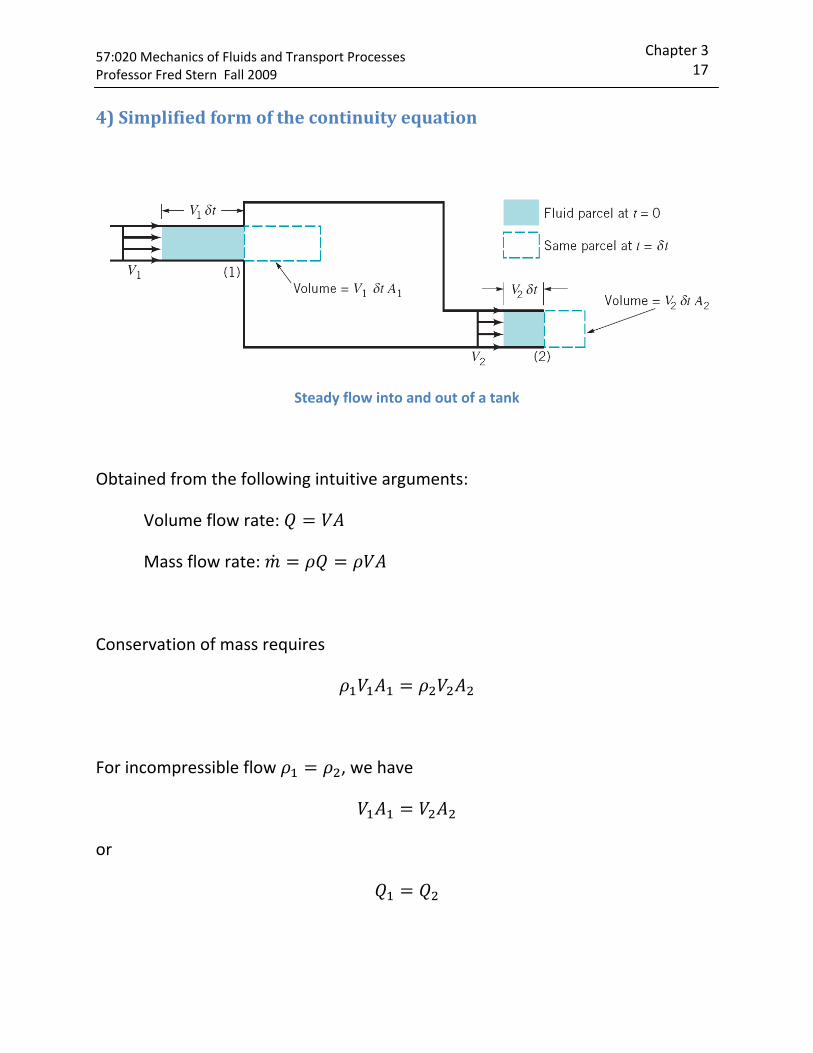
4) Simplified form of the continuity equation
Steady flow into and out of a tank
Obtained from the following intuitive arguments:
Volume flow rate:
Mass flow rate:
Conservation of mass requires
For incompressible flow , we have
or
57:020 MProfessor
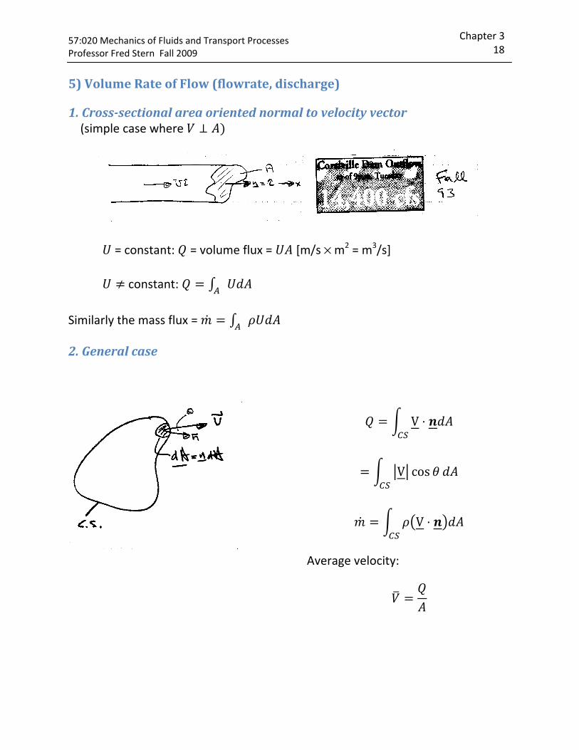
5) Volu
1. Cross (simp
Similarly
2. Gene
echanics of F Fred Stern F
ume Rate
s-sectionaple case wh
= constan
consta
y the mass
eral case
Fluids and TraFall 2009
of Flow (
al area orhere
nt: = vol
ant:
s flux =
nsport Proce
(flowrate,
riented no
ume flux =
esses
, discharg
ormal to v
= [m/s ×
Ave
ge)
velocity ve
× m2 = m3/
erage veloc
ector
/s]
VV cos
Vcity:
Chapte
er 3 18
57:020 Mechanics of Fluids and Transport Processes Professor Fred Stern Fall 2009
Chapter 3 19
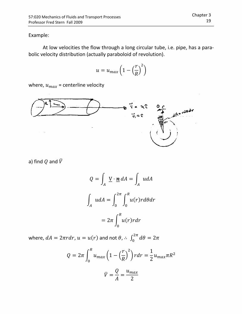
Example:
At low velocities the flow through a long circular tube, i.e. pipe, has a para-bolic velocity distribution (actually paraboloid of revolution).
1
where, = centerline velocity
a) find and
V
2
where, 2 , and not , 2
2 1 12
2
57:020 Mechanics of Fluids and Transport Processes Professor Fred Stern Fall 2009
Chapter 3 20
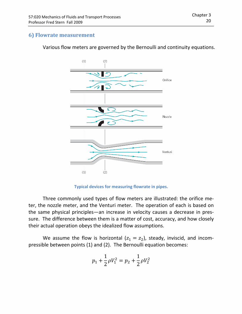
6) Flowrate measurement
Various flow meters are governed by the Bernoulli and continuity equations.
Typical devices for measuring flowrate in pipes.
Three commonly used types of flow meters are illustrated: the orifice me-ter, the nozzle meter, and the Venturi meter. The operation of each is based on the same physical principles—an increase in velocity causes a decrease in pres-sure. The difference between them is a matter of cost, accuracy, and how closely their actual operation obeys the idealized flow assumptions.
We assume the flow is horizontal ( ), steady, inviscid, and incom-pressible between points (1) and (2). The Bernoulli equation becomes: 12 12
57:020 Mechanics of Fluids and Transport Processes Professor Fred Stern Fall 2009
Chapter 3 21
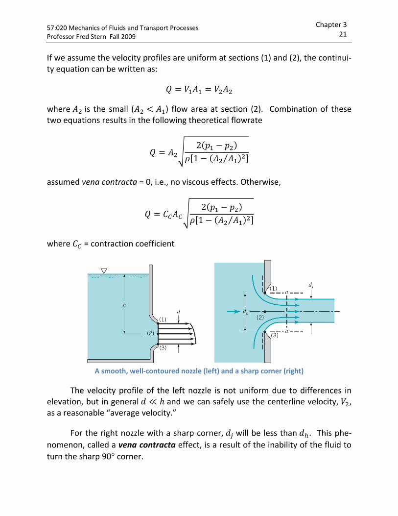
If we assume the velocity profiles are uniform at sections (1) and (2), the continui-ty equation can be written as:
where is the small ( ) flow area at section (2). Combination of these two equations results in the following theoretical flowrate 21 ⁄
assumed vena contracta = 0, i.e., no viscous effects. Otherwise, 21 ⁄
where = contraction coefficient
A smooth, well-contoured nozzle (left) and a sharp corner (right)
The velocity profile of the left nozzle is not uniform due to differences in elevation, but in general and we can safely use the centerline velocity, , as a reasonable “average velocity.”
For the right nozzle with a sharp corner, will be less than . This phe-nomenon, called a vena contracta effect, is a result of the inability of the fluid to turn the sharp 90° corner.
57:020 Mechanics of Fluids and Transport Processes Professor Fred Stern Fall 2009
Chapter 3 22
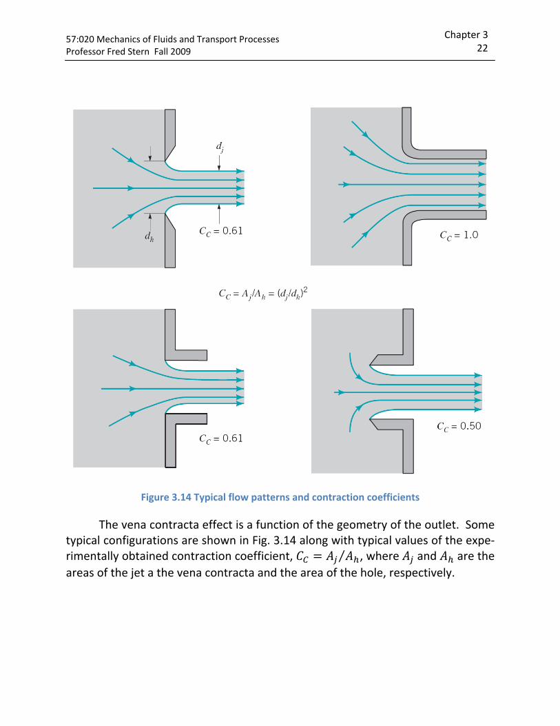
Figure 3.14 Typical flow patterns and contraction coefficients
The vena contracta effect is a function of the geometry of the outlet. Some typical configurations are shown in Fig. 3.14 along with typical values of the expe-rimentally obtained contraction coefficient, ⁄ , where and are the areas of the jet a the vena contracta and the area of the hole, respectively.
57:020 Mechanics of Fluids and Transport Processes Professor Fred Stern Fall 2009
Chapter 3 23
⁄
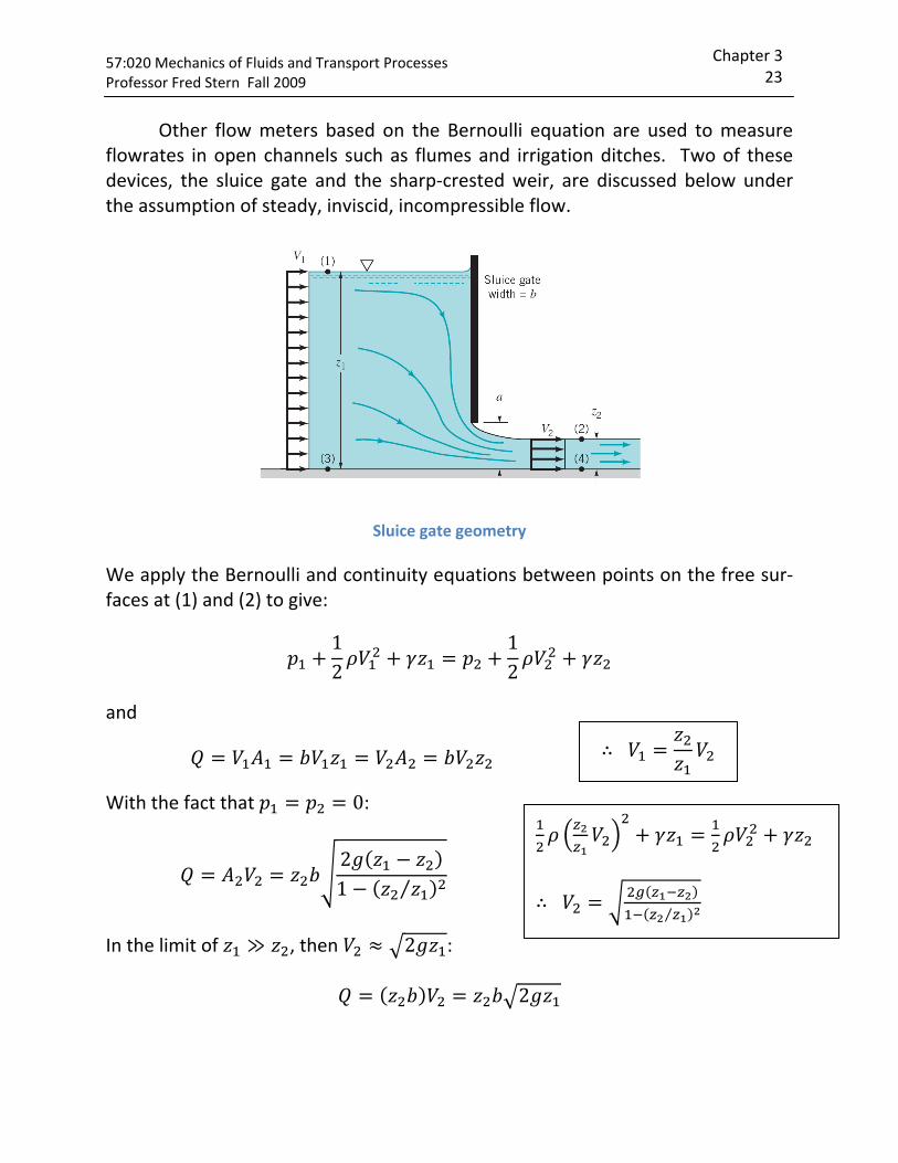
Other flow meters based on the Bernoulli equation are used to measure flowrates in open channels such as flumes and irrigation ditches. Two of these devices, the sluice gate and the sharp-crested weir, are discussed below under the assumption of steady, inviscid, incompressible flow.
Sluice gate geometry
We apply the Bernoulli and continuity equations between points on the free sur-faces at (1) and (2) to give: 12 12
and
With the fact that 0: 21 ⁄
In the limit of , then 2 : 2
57:020 Mechanics of Fluids and Transport Processes Professor Fred Stern Fall 2009
Chapter 3 24
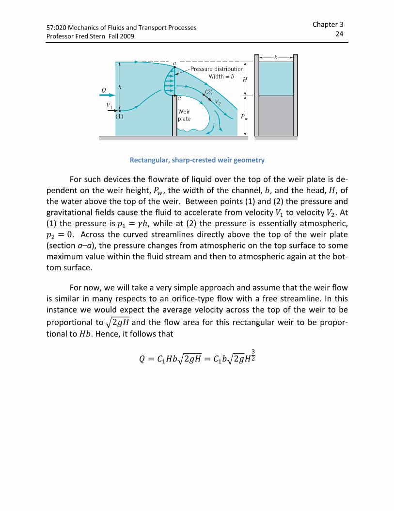
Rectangular, sharp-crested weir geometry
For such devices the flowrate of liquid over the top of the weir plate is de-pendent on the weir height, , the width of the channel, , and the head, , of the water above the top of the weir. Between points (1) and (2) the pressure and gravitational fields cause the fluid to accelerate from velocity to velocity . At (1) the pressure is , while at (2) the pressure is essentially atmospheric, 0. Across the curved streamlines directly above the top of the weir plate (section a–a), the pressure changes from atmospheric on the top surface to some maximum value within the fluid stream and then to atmospheric again at the bot-tom surface.
For now, we will take a very simple approach and assume that the weir flow is similar in many respects to an orifice-type flow with a free streamline. In this instance we would expect the average velocity across the top of the weir to be proportional to 2 and the flow area for this rectangular weir to be propor-tional to . Hence, it follows that 2 2
57:020 Mechanics of Fluids and Transport Processes Professor Fred Stern Fall 2009
Chapter 3 25
3.7 Energy grade line (EGL) and hydraulic grade line (HGL)
This part will be covered later at Chapter 5.
3.8 Limitations of Bernoulli Equation
Assumptions used in the derivation Bernoulli Equation:
(1) Inviscid (2) Incompressible (3) Steady (4) Conservative body force
1) Compressibility Effects:
The Bernoulli equation can be modified for compressible flows. A simple, although specialized, case of compressible flow occurs when the temperature of a perfect gas remains constant along the streamline—isothermal flow. Thus, we consider , where is constant (In general, , , and will vary). An equ-ation similar to the Bernoulli equation can be obtained for isentropic flow of a perfect gas. For steady, inviscid, isothermal flow, Bernoulli equation becomes 12
The constant of integration is easily evaluated if , , and are known at some location on the streamline. The result is
2 ln 2
57:020 Mechanics of Fluids and Transport Processes Professor Fred Stern Fall 2009
Chapter 3 26
2) Unsteady Effects:
The Bernoulli equation can be modified for unsteady flows. With the inclu-sion of the unsteady effect ( ⁄ 0) the following is obtained: 0 (along a streamline)
For incompressible flow this can be easily integrated between points (1) and (2) to give
(along a streamline)
3) Rotational Effects
Care must be used in applying the Bernoulli equation across streamlines. If the flow is “irrotational” (i.e., the fluid particles do not “spin” as they move), it is appropriate to use the Bernoulli equation across streamlines. However, if the flow is “rotational” (fluid particles “spin”), use of the Bernoulli equation is re-stricted to flow along a streamline.
4) Other Restrictions
Another restriction on the Bernoulli equation is that the flow is inviscid. The Bernoulli equation is actually a first integral of Newton's second law along a streamline. This general integration was possible because, in the absence of visc-ous effects, the fluid system considered was a conservative system. The total energy of the system remains constant. If viscous effects are important the sys-tem is nonconservative and energy losses occur. A more detailed analysis is needed for these cases.
The Bernoulli equation is not valid for flows that involve pumps or turbines. The final basic restriction on use of the Bernoulli equation is that there are no mechanical devices (pumps or turbines) in the system between the two points along the streamline for which the equation is applied. These devices represent sources or sinks of energy. Since the Bernoulli equation is actually one form of the energy equation, it must be altered to include pumps or turbines, if these are present.