Chapter: 3 · 3.5.Incompatible modes Incompatible modes, or incompatible displacemets, is a method...

Department ofMathematics

University of Oslo

Subdomain interior nodes

Subdomain boundary nodes Subdomain boundaries

Mek 4560Torgeir Rusten

Contents

// ..

/ .

of 35

Go Back

Close

Quit

Chapter: 3

MEK4560The Finite Element Method in

Solid Mechanics II(January 31, 2008)

Torgeir Rusten

(E-post:[email protected])

E-post:[email protected]

E-post:[email protected]


University of Oslo




Contents

// ..

/ .

of 35

Go Back

Close

Quit

Contents

3 Variational crimes [Strang and Fix, 1973] 33.1 Full integration . . . . . . . . . . . . . . . . . . . . . . . . . . . . . . . . . . . . 43.2 Selective reduced integration . . . . . . . . . . . . . . . . . . . . . . . . . . . . 43.3 Uniform reduced integration . . . . . . . . . . . . . . . . . . . . . . . . . . . . . 83.4 Mindlin-Reissner beams . . . . . . . . . . . . . . . . . . . . . . . . . . . . . . . 83.5 Incompatible modes . . . . . . . . . . . . . . . . . . . . . . . . . . . . . . . . . 93.6 Membrane elements . . . . . . . . . . . . . . . . . . . . . . . . . . . . . . . . . 12

3.6.1 Rotational degrees of freedom . . . . . . . . . . . . . . . . . . . . . . . . 133.6.2 Hybrid formulations . . . . . . . . . . . . . . . . . . . . . . . . . . . . . 13

3.7 The Patch test and convergence . . . . . . . . . . . . . . . . . . . . . . . . . . . 143.7.1 Background . . . . . . . . . . . . . . . . . . . . . . . . . . . . . . . . . . 143.7.2 The Patch test . . . . . . . . . . . . . . . . . . . . . . . . . . . . . . . . 15

3.8 Element quality . . . . . . . . . . . . . . . . . . . . . . . . . . . . . . . . . . . . 183.9 Bjelke (PLANE42) . . . . . . . . . . . . . . . . . . . . . . . . . . . . . . . . . . 203.10 I-bjelke (SOLID45) . . . . . . . . . . . . . . . . . . . . . . . . . . . . . . . . . . 24

A References 35


University of Oslo




Contents

// ..

/ .

of 35

Go Back

Close

Quit

3. Variational crimes [Strang and Fix, 1973]

In this chapter we introduce some “tricks of the trade” used to improve some finite elements.First selective reduced integration is motivated by an example. Then an application of uniformreduced integration is mentioned, see [Cook et al., 2002][1], Chapter 6.8.

Another method to improve elements for bending dominated analysis is incompatible modes,see [Cook et al., 2002][1], Chapter 6.6.

We also mention some “improved” element formulations, elements with rotational degrees offreedom and hybrid elements, [Cook et al., 2002][1] 3.10, 4.10.

All the above mentioned methods are called Variational crimes in Strang and Fix [Strang and Fix, 1973][3].

Since the basic requirements for convergence are violated an alternative criteria is introduce,named the patch test, [Cook et al., 2002] 6.13.

Element evaluation are mentioned briefly, see [Cook et al., 2002][1] 6.11.

[1] R. D. Cook, D. S. Malkus, M. E. Plesha, and R. J. Witt. Concepts and Applications of Finite ElementAnalysis. Number ISBN: 0-471-35605-0. John Wiley & Sons, Inc., 4th edition, October 2002.

[3] G. Strang and G. J. Fix. An Analysis of the Finite Element Method. Prentice-Hall, Englewood Cliffs, NewJersey, 1973.


University of Oslo




Contents

// ..

/ .

of 35

Go Back

Close

Quit

3.1. Full integration

If an integration rule are sufficiently accurate to integrate the stiffness coefficients exactly therule is called a full integration rule, see [Cook et al., 2002][1], Chapter 6.8. Quadrilateral andhexahedral elements are undistorted if they are rectangular and mid side nodes, if present, areuniformly spaced along straight edges.

3.2. Selective reduced integration

Selective integration of the shear term was introduce in the begin of the seventies in order toimprove the accuracy of lower order square elements applied to bending dominated problems.To motivate it we consider a plane stress model and a bending dominated problem.

Pure bending is defined by σxx ∝ y. The displacement field is given by

u = x y

v = −12(x2 + νy2

)



University of Oslo




Contents

// ..

/ .

of 35

Go Back

Close

Quit

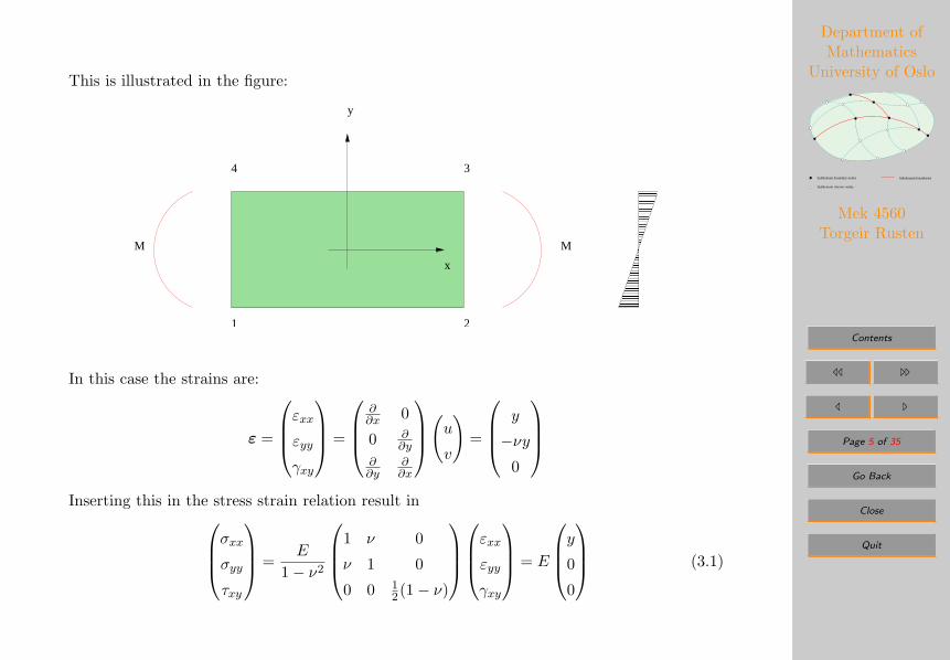
This is illustrated in the figure:

��

��

4 3

21

M M

x

y

In this case the strains are:

ε =

εxxεyyγxy

=

∂∂x 0

0 ∂∂y

∂∂y

∂∂x

(u

v

)=

y

−νy0

Inserting this in the stress strain relation result inσxxσyy

τxy

=E

1− ν2

1 ν 0

ν 1 0

0 0 12(1− ν)

εxxεyyγxy

= E

y00

(3.1)


University of Oslo




Contents

// ..

/ .

of 35

Go Back

Close

Quit

and the strain energy becomes

E

2

∫ 1

−1

∫ 1

−1y2 dx dy =

23E (3.2)

Then, consider a bilinear element with nodes in (−1,−1), (1,−1), (1, 1) and (−1, 1). Thebilinear basis functions are

N1(x, y) =14

(1− x)(1− y) (3.3)

N2(x, y) =14

(1 + x)(1− y) (3.4)

N3(x, y) =14

(1 + x)(1 + y) (3.5)

N4(x, y) =14

(1− x)(1 + y) (3.6)

The finite element interpolation of u is denoted uh and uh = xy, i.e. is equal to u. The valueof v at all the nodes are −1

2(1 + ν), hence vh = −12(1 + ν). Thus, the strains becomes

ε =

εxxεyyτxy

=

y0x

(3.7)

Inserting into the stress strain relations result inσxxσyy

xy

=E

1− ν2

y

νy12(1− ν)x

(3.8)


University of Oslo




Contents

// ..

/ .

of 35

Go Back

Close

Quit

and the strain energy becomes

E

2(1− ν2)

∫ 1

−1

∫ 1

−1y2 +

12

(1− ν)x2 dx dy =23

E

1− ν2+

23G (3.9)

Comparing this to (3.2) we note the appearance of the shear term, in addition to the membraneterm. The unphysical shear therm absorb part of the energy, and the finite element solutionappears to stiff. Note that if the shear term is integrated numerically by a one point integrationrule, where the evaluation point is at the origin the shear term vanish.

This motivates the use of reduced shear integration. Note that this does not prove thatreduced integration improve the computed results! It is an indication that it is worth trying.The experience in computation mechanics, however, is that reduced integration of the shearterm improve the numerical results.


University of Oslo




Contents

// ..

/ .

of 35

Go Back

Close

Quit

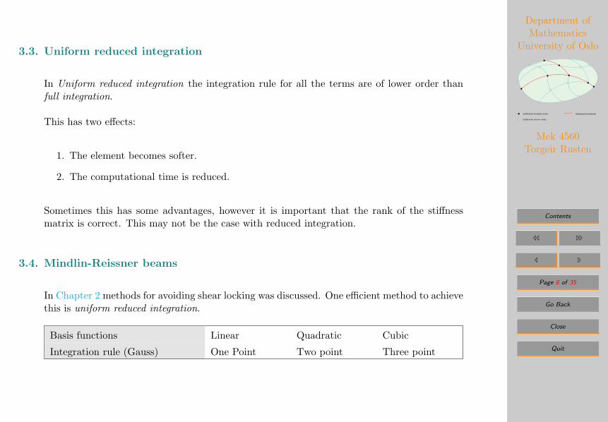
3.3. Uniform reduced integration

In Uniform reduced integration the integration rule for all the terms are of lower order thanfull integration.

This has two effects:

1. The element becomes softer.

2. The computational time is reduced.

Sometimes this has some advantages, however it is important that the rank of the stiffnessmatrix is correct. This may not be the case with reduced integration.

3.4. Mindlin-Reissner beams

In Chapter 2 methods for avoiding shear locking was discussed. One efficient method to achievethis is uniform reduced integration.

Basis functions Linear Quadratic Cubic

Integration rule (Gauss) One Point Two point Three point


University of Oslo




Contents

// ..

/ .

of 35

Go Back

Close

Quit

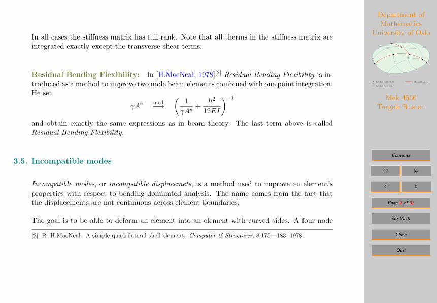
In all cases the stiffness matrix has full rank. Note that all therms in the stiffness matrix areintegrated exactly except the transverse shear terms.

Residual Bending Flexibility: In [H.MacNeal, 1978][2] Residual Bending Flexibility is in-troduced as a method to improve two node beam elements combined with one point integration.He set

γAsmed−→

(1γAs

+h2

12EI

)−1

and obtain exactly the same expressions as in beam theory. The last term above is calledResidual Bending Flexibility.

3.5. Incompatible modes

Incompatible modes, or incompatible displacemets, is a method used to improve an element’sproperties with respect to bending dominated analysis. The name comes from the fact thatthe displacements are not continuous across element boundaries.

The goal is to be able to deform an element into an element with curved sides. A four node

[2] R. H.MacNeal. A simple quadrilateral shell element. Computer & Structurer, 8:175—183, 1978.


University of Oslo




Contents

// ..

/ .

of 35

Go Back

Close

Quit

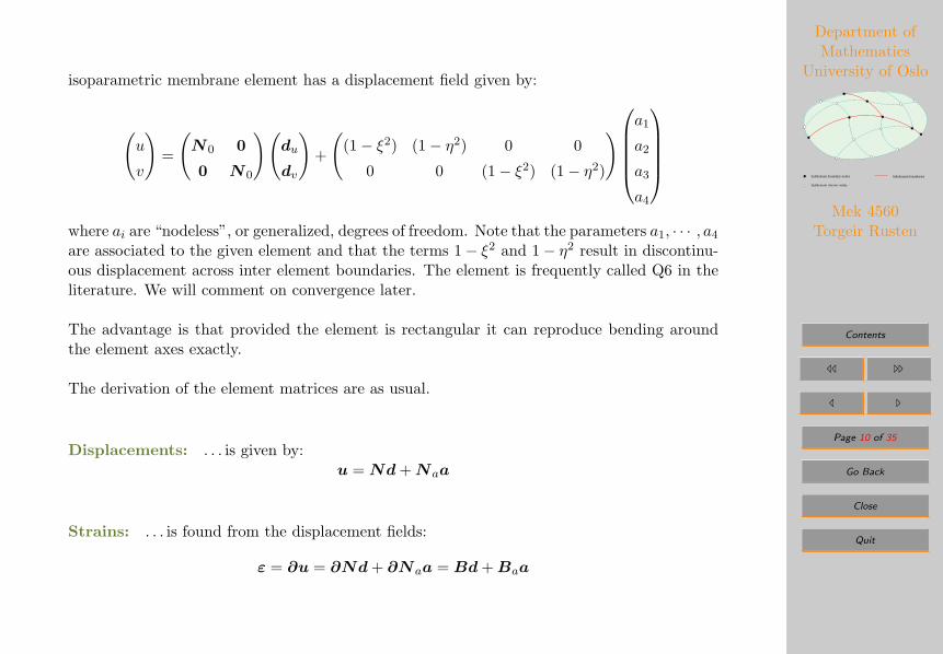
isoparametric membrane element has a displacement field given by:

(u

v

)=

(N0 0

0 N0

)(du

dv

)+

((1− ξ2) (1− η2) 0 0

0 0 (1− ξ2) (1− η2)

)a1

a2

a3

a4

where ai are “nodeless”, or generalized, degrees of freedom. Note that the parameters a1, · · · , a4

are associated to the given element and that the terms 1− ξ2 and 1− η2 result in discontinu-ous displacement across inter element boundaries. The element is frequently called Q6 in theliterature. We will comment on convergence later.

The advantage is that provided the element is rectangular it can reproduce bending aroundthe element axes exactly.

The derivation of the element matrices are as usual.

Displacements: . . . is given by:u = Nd+Naa

Strains: . . . is found from the displacement fields:

ε = ∂u = ∂Nd+ ∂Naa = Bd+Baa


University of Oslo




Contents

// ..

/ .

of 35

Go Back

Close

Quit

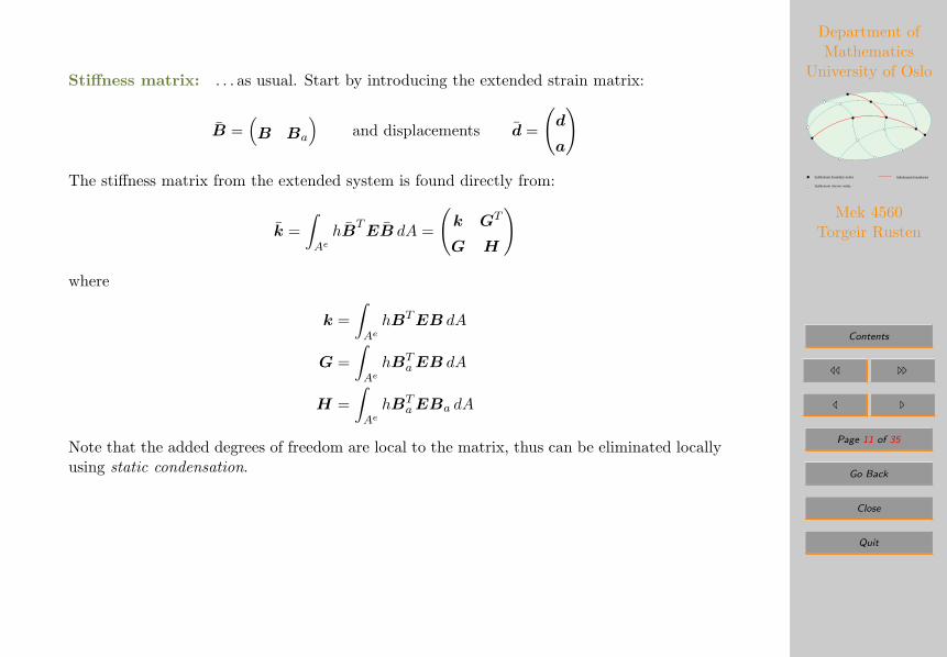
Stiffness matrix: . . . as usual. Start by introducing the extended strain matrix:

B =(B Ba

)and displacements d =

(d

a

)

The stiffness matrix from the extended system is found directly from:

k =∫Ae

hBTEB dA =

(k GT

G H

)

where

k =∫Ae

hBTEB dA

G =∫Ae

hBTaEB dA

H =∫Ae

hBTaEBa dA

Note that the added degrees of freedom are local to the matrix, thus can be eliminated locallyusing static condensation.


University of Oslo




Contents

// ..

/ .

of 35

Go Back

Close

Quit

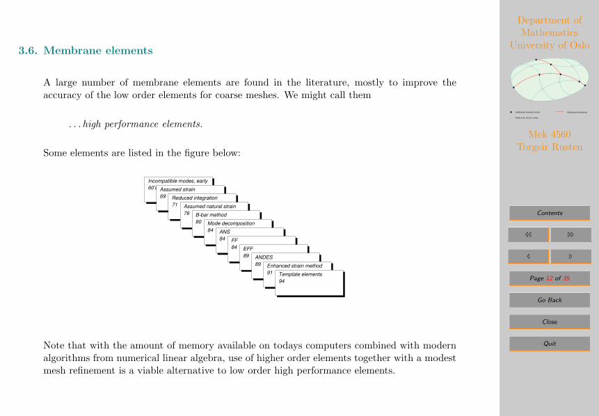
3.6. Membrane elements

A large number of membrane elements are found in the literature, mostly to improve theaccuracy of the low order elements for coarse meshes. We might call them

. . . high performance elements.

Some elements are listed in the figure below:

Incompatible modes, early60’s Assumed strain

69 Reduced integration71 Assumed natural strain

76 B-bar method80 Mode decomposition

84 ANS84 FF

84 EFF89 ANDES

89 Enhanced strain method91 Template elements

94

Note that with the amount of memory available on todays computers combined with modernalgorithms from numerical linear algebra, use of higher order elements together with a modestmesh refinement is a viable alternative to low order high performance elements.


University of Oslo




Contents

// ..

/ .

of 35

Go Back

Close

Quit

3.6.1. Rotational degrees of freedom

In addition to the usual translation degrees of freedom one use rotations in the corner nodesas nodal degrees of freedom. We mention two interesting aspects of this:

1. Improved accuracy of three and four node elements

2. Useful in shell formulations

In[Cook et al., 2002][1] a modification of the quadratic elements for plane elasticity is consid-ered. Here the six displacements degrees of freedom at the mid side nodes are replaced withthree rotational degrees of freedom at the corner nodes.

3.6.2. Hybrid formulations

Hybrid formulations are not based on the principle of complementary strain energy.

In some cases the hybrid formulation is build on the assumptions:

1. the stress field σ is in equilibrium in the element

2. the displacements ud are defined on inter element boundaries



University of Oslo




Contents

// ..

/ .

of 35

Go Back

Close

Quit

3.7. The Patch test and convergence

3.7.1. Background

In order for the finite element method to be useful the linear systems must be nonsingular, i.e.solvable, and the finite element approximation uh defined using the basis functions and thecomputed nodal degrees of freedom must “converge” to the exact solution u when the meshis refined. The subscript h is a parameter measuring the mesh size of the elements in themesh, typically the smallest length of an element edge or the radius of the smallest inscribedcircle/ball. One say that uh “converge” towards u if uh becomes “close” to u whenever themesh size h approach zero. One way to measure the difference of two functions is to introducea norm. One way to introduce a norm is to integrate the square of the function:

‖u2‖ =∫Vu2 dV (3.10)

In order to measure error in finite element methods derivatives are often introduced int theintegral, since on would like to control certain derivatives of the functions too.

Basic requirement:

1. The basis functions must have complete polynomials of degree m. Note: for membraneelements linear polynomials are required.

2. Compatibility functions across inter element boundaries, i.e. (m − 1)-continuity. Note:for membrane elements the displacements must be continuous.


University of Oslo




Contents

// ..

/ .

of 35

Go Back

Close

Quit

3. m−th derivatives of field variables must be represented when the element size becomessmall. Note: for membrane elements constant strains must be represented exactly.

In addition one would like elements to be:

4. Geometric invariant. I.e. the solution should not depend on the orientation of the globalcoordinate system.

In the next Chapter methods where the compatibility condition can be relaxed.

3.7.2. The Patch test

Irons, [Bazeley et al., 1965], in 1965 suggested a numerical test to check the validity of anelement formulation. If this test, called the Patch test, is satisfied it is verified that thesolution convergence to the correct solution. This statement is, and has been, controversialbut the test is accepted in the engineering community.

The Patch test (procedure): . . . is a necessary and sufficient for convergence [Taylor et al., 1986][4].We check that all rigid-body motions and constant strains are exactly represented for a set of

[4] R. L. Taylor, O. C. Zienkiewicz, J. C. Simo, and A. C. H. Chan. The patch test — A condition for assessingFEM convergence. International Journal for Numerical Methods in Engineering, 22:39–62, 1986.


University of Oslo




Contents

// ..

/ .

of 35

Go Back

Close

Quit

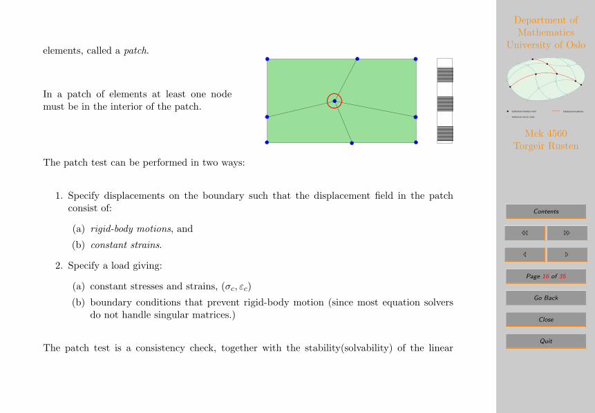
elements, called a patch.

In a patch of elements at least one nodemust be in the interior of the patch.

��

��

The patch test can be performed in two ways:

1. Specify displacements on the boundary such that the displacement field in the patchconsist of:

(a) rigid-body motions, and

(b) constant strains.

2. Specify a load giving:

(a) constant stresses and strains, (σc, εc)

(b) boundary conditions that prevent rigid-body motion (since most equation solversdo not handle singular matrices.)

The patch test is a consistency check, together with the stability(solvability) of the linear


University of Oslo




Contents

// ..

/ .

of 35

Go Back

Close

Quit

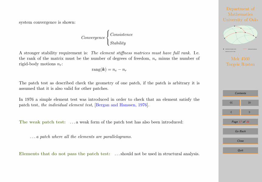
system convergence is shown:

Convergence

Consistence

Stability

A stronger stability requirement is: The element stiffness matrices must have full rank. I.e.the rank of the matrix must be the number of degrees of freedom, ne minus the number ofrigid-body motions nr:

rang(k) = ne − nr

The patch test as described check the geometry of one patch, if the patch is arbitrary it isassumed that it is also valid for other patches.

In 1976 a simple element test was introduced in order to check that an element satisfy thepatch test, the individual element test, [Bergan and Hanssen, 1976].

The weak patch test: . . . a weak form of the patch test has also been introduced:

. . . a patch where all the elements are parallelograms.

Elements that do not pass the patch test: . . . should not be used in structural analysis.


University of Oslo




Contents

// ..

/ .

of 35

Go Back

Close

Quit

3.8. Element quality

The goal is to obtain sufficient accuracy of the analysis as efficiently as possible. Usually onethink of efficiency as computational efficiency, but it also makes sense to consider the man-timeinvolved.

Note: The quality of a finite element analysis depend on the chosen finite element and also anthe geometry of the elements. An a-priori, i.e. without knowledge of the solution, a qualitativeassessment of element quality is impossible.

Fortunately, in connection to structural analysis a-priori knowledge of the solution exist andexperience in the choice of elements are gained over the years. The comments below are relatedto structural analysis.

1. Square elements is better than triangular elements.

2. Geometricly “distorted” elements result in a stiffer element.

For lower order elements:

1. Shear locking can be a problem and bending is poorly represented.

For nine node Lagrangian and eight node Serendipity elements:


University of Oslo




Contents

// ..

/ .

of 35

Go Back

Close

Quit

1. Rectangular elements give identical results.

2. 3× 3 integration is stiffer than 2× 2.

3. 8 node element are more sensitive to the geometry.

Conclusion: The ideal element is

1. Quadratic,

Use of “bad” elements:

. . . concentrate the “bad” elements.

. . . in doubt? Compute on several different meshes, mesh refinement. (Adaptive methods?).


University of Oslo




Contents

// ..

/ .

of 35

Go Back

Close

Quit

3.9. Bjelke (PLANE42)

1m

y

E=1000

5m

x

q=5N

Problem: Den fast innspente bjelken som er vist i figuren skal modelleres med 4-knutepunktsmembranelementer som har 2 frihetsgrader pr. knutepunkt. Bjelken skal diskretiseres slik atarealene til alle elementer skal være 0.25× 0.25m2 (dvs. 80 elementer).

Foreta elementmetodeanalyse der lasten paføres som:

i) vist i figuren (flatestrekk).

ii) 5 punktlaster (P = 1kN) pa de fem endeknutepunktene.

Department of Mathematics

University of Oslo



Mek 4560

Torgeir Rusten

Contents

// ..

/ .

of 35

Go Back

Close

Quit

Hvilken av disse to belastninger modellerer det som figuren viser mest nøyaktig?

Hva er σx og εx ved x = 2.5m, y = 0.5m og x = 4.5m, y = 0.5m? Kommenter nøyaktighetenav disse verdiene.

Løsning:

/BATCH,LIST

/FILNAM,ex413

/TITLE,Lineær statisk analyse av en bjelke

/PREP7 ! Preprossessoren

ET,1,42 ! PLANE42 membranelementer (plan spenning)

MP,EX,1,1e3 ! E-modulen

!Geometri ("solid modelling")

K,1 ! origo

K,2,0,1e3

K,3,5e3,1e3

K,4,5e3,0

A,1,2,3,4 ! Areal lages (linjer lages automatisk)

!Inndeling i elementer

LESIZE,ALL,250

AMESH,1

FINISH

/SOLU

ANTYPE,STATIC

NSEL,S,LOC,X,0 ! Velger alle knutepunkt med x-koord lik null

D,ALL,ALL ! Opplagring ved innspenningen

NSEL,S,LOC,X,5e3 ! Velger alle knutepunkt med x-koord lik 5m

ESLN,S,0 ! Velger alle elementer med minst ett knutepunkt i valgt sett


University of Oslo




Contents

// ..

/ .

of 35

Go Back

Close

Quit

SFE,ALL,2,PRES,,-5

ALLSEL

LSWRITE,1

SFEDEL,ALL,ALL,ALL ! Fa bort den jevnt fordelte lasten

NSEL,S,LOC,X,5e3

F,ALL,FX,1e3 ! Punktbelastningen

ALLSEL

LSWRITE,2

LSSOLVE,1,2 ! Løsningsprosedyren

FINISH

/POST1

SET,1,1 ! Last inn analyseresultatene for jevnt fordelt last

PLDISP,1 ! Deformert geometri

NSEL,S,NODE,,NODE(5000,500,0)

PRNSOL,S,X

SET,2,1 ! Resultat for punktbelastningen

PRNSOL,S,X

ALLSEL

FINISH

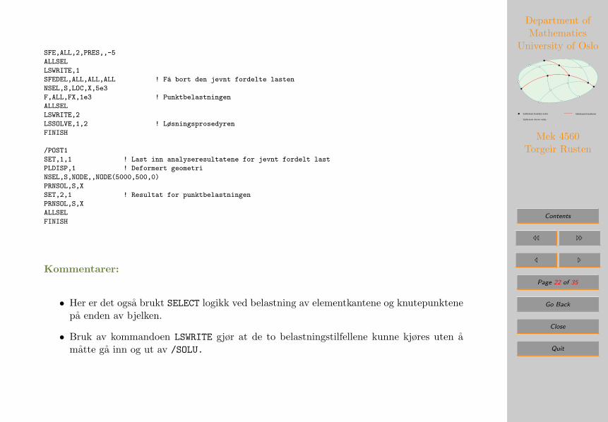
Kommentarer:

• Her er det ogsa brukt SELECT logikk ved belastning av elementkantene og knutepunktenepa enden av bjelken.

• Bruk av kommandoen LSWRITE gjør at de to belastningstilfellene kunne kjøres uten amatte ga inn og ut av /SOLU.


University of Oslo




Contents

// ..

/ .

of 35

Go Back

Close

Quit

Svar pa spørsmalene Fra den deformerte geometrien til de to lasttilfellene ser man atbelastningen med flatestrekk er a foretrekke fordi endetversnittet forblir rett.

Belastningene ga følgende σx og εx verdier:

Belastning

Flatestrekk Punktlast

Kn. pkt. 2.5, 0.5 σx = 5.000 εx = 0.5× 10−2 σx = 4.999 εx = 0.4999× 10−2

koord. 4.5, 0.5 σx = 5.000 εx = 0.5× 10−2 σx = 4.219 εx = 0.4069× 10−2

Unøyaktigheten av σx og εx med punktbelastningen viser tydelig St. Venants effekten - jolengre bort fra enden, sa blir spennings- og tøyningsfordelingen mer lik de riktige verdier.


University of Oslo




Contents

// ..

/ .

of 35

Go Back

Close

Quit

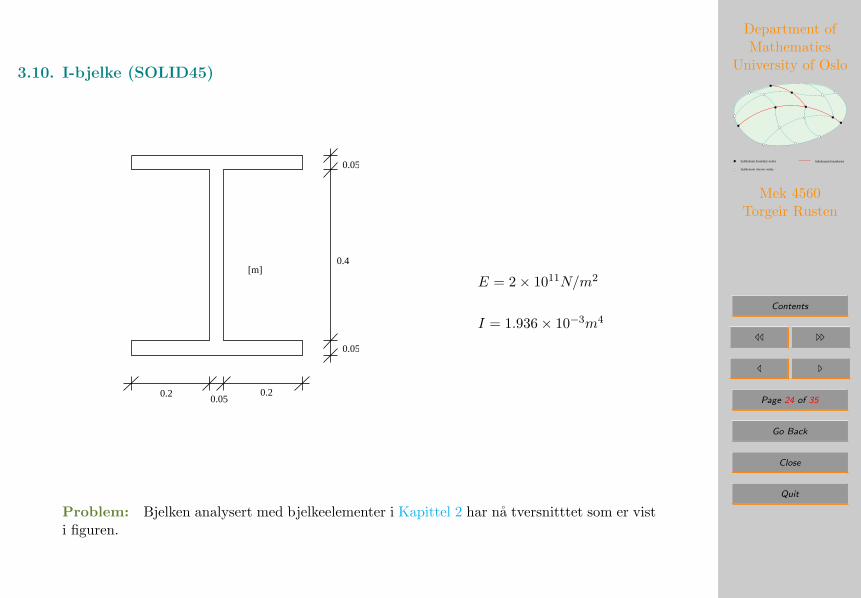
3.10. I-bjelke (SOLID45)

0.20.05

0.2

0.05

0.4

0.05

[m]E = 2× 1011N/m2

I = 1.936× 10−3m4

Problem: Bjelken analysert med bjelkeelementer i Kapittel 2 har na tversnitttet som er visti figuren.

Department of Mathematics

University of Oslo



Mek 4560

Torgeir Rusten

Contents

// ..

/ .

of 35

Go Back

Close

Quit

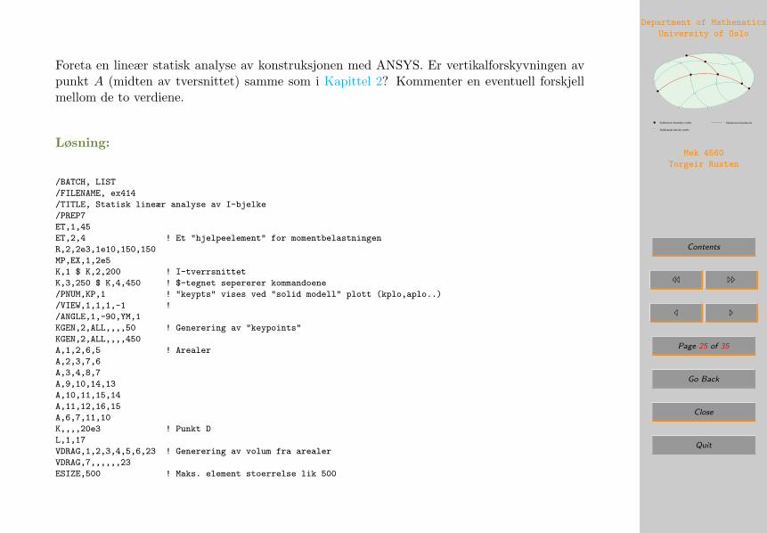
Foreta en lineær statisk analyse av konstruksjonen med ANSYS. Er vertikalforskyvningen avpunkt A (midten av tversnittet) samme som i Kapittel 2? Kommenter en eventuell forskjellmellom de to verdiene.

Løsning:

/BATCH, LIST

/FILENAME, ex414

/TITLE, Statisk lineær analyse av I-bjelke

/PREP7

ET,1,45

ET,2,4 ! Et "hjelpeelement" for momentbelastningen

R,2,2e3,1e10,150,150

MP,EX,1,2e5

K,1 $ K,2,200 ! I-tverrsnittet

K,3,250 $ K,4,450 ! $-tegnet sepererer kommandoene

/PNUM,KP,1 ! "keypts" vises ved "solid modell" plott (kplo,aplo..)

/VIEW,1,1,1,-1 !

/ANGLE,1,-90,YM,1

KGEN,2,ALL,,,,50 ! Generering av "keypoints"

KGEN,2,ALL,,,,450

A,1,2,6,5 ! Arealer

A,2,3,7,6

A,3,4,8,7

A,9,10,14,13

A,10,11,15,14

A,11,12,16,15

A,6,7,11,10

K,,,,20e3 ! Punkt D

L,1,17

VDRAG,1,2,3,4,5,6,23 ! Generering av volum fra arealer

VDRAG,7,,,,,,23

ESIZE,500 ! Maks. element stoerrelse lik 500


University of Oslo




Contents

// ..

/ .

of 35

Go Back

Close

Quit

VMESH,ALL

TYPE,2 $ REAL,2 ! "hjelpeelementet"

E,NODE(200,50,12e3),NODE(200,450,12e3) ! ved punkt C

NUMMRG,ALL ! To noder paa samme punkt blir en

NUMCMP,ALL ! Komprimer numerering

NSEL,S,NODE,,108 ! Bjelkeelement med 2 knutepunkter

NSEL,A,NODE,,355

CERIG,355,ALL ! Kobling av bjelke og volumelementer

NSEL,ALL

FINISH

/SOLU

NSEL,,LOC,Y,0 ! "select" for aa paafoere last og sette

NSEL,R,LOC,Z,4e3 ! Grensebetingelser

D,ALL,UY,,,,,UX,UZ ! Fastholdt pa undersiden av bjelken ved B

NSEL,,LOC,Y,0

NSEL,R,LOC,Z,20e3 ! ved D

D,ALL,UY,,,,,UX

NSEL,ALL

NSEL,S,LOC,Y,460,500

NSEL,R,LOC,Z,0,3900

ESLN,S,0 ! Oversiden av AB

SFE,ALL,1,PRES,,-.3333333

ALLSEL

F,NODE(200,450,12e3),MX,12e9 ! Momentbelastningen

SOLVE

SAVE

FINISH

/POST1

SET

/SHOW, ex414pl

PLDISP,1

PRERR

FINISH


University of Oslo




Contents

// ..

/ .

of 35

Go Back

Close

Quit

Svar/kommentarer: Et bjelkeelement er brukt som ”hjelpeelement” for paføring av mo-mentbelastningen. Bjelkeelementets frihetsgrader er koblet sammen med volumelementenegjennom kommandoen CERIG (som lager koblingsligninger - jfr. kurset MEK4550 ).

Nei, nedbøyningen av punkt A (ca. 95mm) er ikke den samme som i Kapittel 2 .

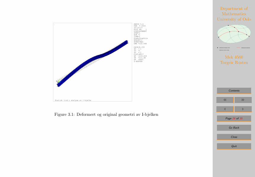
Denne konstruksjon er mye stivere (enn den i Kapittel 2). PRERR kommandoen gir en tilnærmetverdi (i %) av feilen som darlig ”mesh” (geometri,type og inndeling av elementene) i konstruk-sjonen utgjør i resultatet. Denne verdien i dette ekempelet er pa 49.645% - som er veldig høy.Feil kan ogsa oppsta ved maten punktbelastningen paføres. Den deformerte bjelken vises ifiguren nedenfor.


University of Oslo




Contents

// ..

/ .

of 35

Go Back

Close

Quit

ANSYS 5.6FEB 9 200322:10:13PLOT NO. 1DISPLACEMENTSTEP=1SUB =1TIME=1PowerGraphicsEFACET=1AVRES=MatDMX =122.568

1

XY

Z

DSCA=8.159XV =-1YV =1ZV =-1DIST=8017XF =219.218YF =111.38ZF =9921Z-BUFFER

Statisk lind r analyse av I-bjelke

Figure 3.1: Deformert og original geometri av I-bjelken


University of Oslo




Contents

// ..

/ .

of 35

Go Back

Close

Quit

Øving 3.1Hva er Patch testen, og hva er formalet med denne testen?

Sett opp et komplett Patch test problem for et stavelement, der alle randkrav settes pa somforeskrevne forskyvninger. Angi hva som indikerer om testen er oppfylt eller ikke. Tøyningsrelasjonen,materialloven og den totale potensielle energien for stavproblemet er gitt ved:

εxx =du

dxNxx = EAεxx

Π(u) =12

∫`Nxxεxx dx−

∫`qu dx

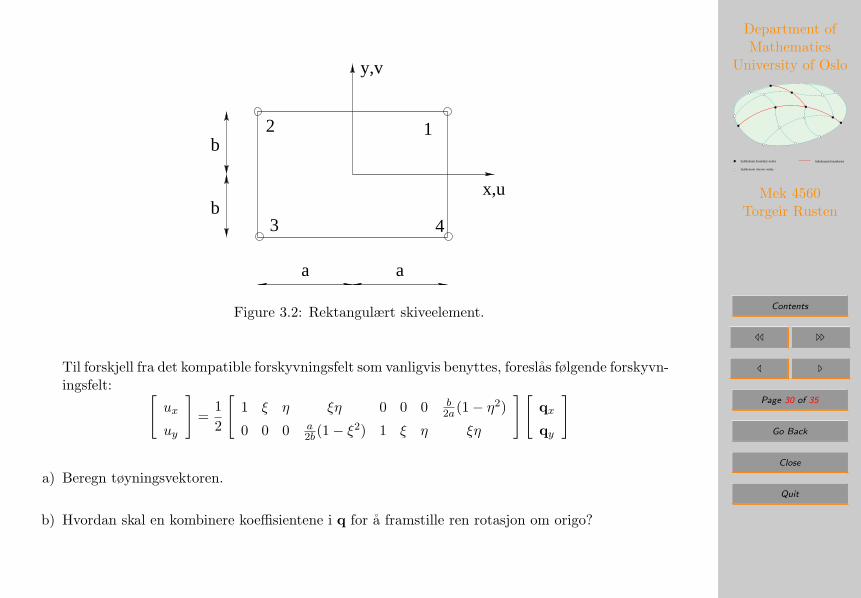
Øving 3.2Figuren viser et rektangulært element med 8 frihetsgrader.


University of Oslo




Contents

// ..

/ .

of 35

Go Back

Close

Quit

x,u

y,v

12

3 4

a

b

a

b

Figure 3.2: Rektangulært skiveelement.

Til forskjell fra det kompatible forskyvningsfelt som vanligvis benyttes, foreslas følgende forskyvn-ingsfelt: [

ux

uy

]=

12

[1 ξ η ξη 0 0 0 b

2a(1− η2)

0 0 0 a2b(1− ξ

2) 1 ξ η ξη

][qxqy

]

a) Beregn tøyningsvektoren.

b) Hvordan skal en kombinere koeffisientene i q for a framstille ren rotasjon om origo?


University of Oslo




Contents

// ..

/ .

of 35

Go Back

Close

Quit

c) Studer elementets egenskaper ved ren bøying om de to aksene. Sammenlign resultatet med etvanlig rektangulært element med 8 frihetsgrader.

d) Beregn stivhetsmatrisene kq for de to elementene. Kan man av dette slutte noe om størrelsenav forskyvningene ved beregning av de to forskjellige matrisene?

Øving 3.3Figuren viser et volumelement med 8 knutepunkter.

1

2 34

5

6

78

2 3

4

5

6 7

8

xz

y

1η

ξ

ζ

Figure 3.3: Isoparametrisk attenoderselement.

a) Finn N uttrykket ved η, ξ, ζ

b) Uttrykk forskyvningene i elementet ved hjelp av de generaliserte forskyvningsmønstre N q


University of Oslo




Contents

// ..

/ .

of 35

Go Back

Close

Quit

c) Finn de tilhørende tøyningene ε.

d) Klassifiser de generaliserte forskyvningsmønsterene i N q etter:

– Stivlegememønstre.

– Konstante tøyningsmønstre.

– Høyere ordens mønstre.

e) Vis hvordan Jakobimatrisen ser ut. (∆ηξζ = J∆xyz)

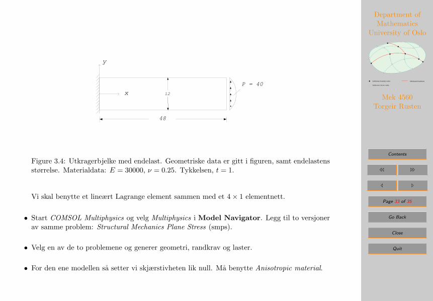
Øving 3.4I denne oppgaven skal vi benytte COMSOL Multiphysics og multi fysikk modellering. Vi skaligjen se pa utkragebjelken fra Kapittel 1 sammen med redusert skjær integrasjon. Problemeter vist i Figure 3.4.


University of Oslo




Contents

// ..

/ .

of 35

Go Back

Close

Quit

x 12

y

P = 40

48

Figure 3.4: Utkragerbjelke med endelast. Geometriske data er gitt i figuren, samt endelastensstørrelse. Materialdata: E = 30000, ν = 0.25. Tykkelsen, t = 1.

Vi skal benytte et lineært Lagrange element sammen med et 4× 1 elementnett.

• Start COMSOL Multiphysics og velg Multiphysics i Model Navigator. Legg til to versjonerav samme problem: Structural Mechanics Plane Stress (smps).

• Velg en av de to problemene og generer geometri, randkrav og laster.

• For den ene modellen sa setter vi skjærstivheten lik null. Ma benytte Anisotropic material.


University of Oslo




Contents

// ..

/ .

of 35

Go Back

Close

Quit

• For den andre modellen sa setter vi de komponenten som ikke er knyttet til skjær lik null. Hervelger vi ogsa en redusert integrasjon for elementet, ettpunkts integrasjon.

• Vi ma koble de to lingningssetene sammen. Det gjør vi for hele domenet.

• Hvordan sammenligner resultatene med de for full integrasjon.


University of Oslo




Contents

// ..

/ .

of 35

Go Back

Close

Quit

A. References

[Bazeley et al., 1965] Bazeley, G. P., Cheung, Y. K., Irons, B. M., and Zienkiewicz, O. C.(1965). Triangular elements in bending — Conforming and non-conforming solutions. InProceedings of Conference on Matrix Methods in Structural Mechanics, Ohio. Air ForceInstitute of Technology, Wright Patterson Air Force Base.

[Bergan and Hanssen, 1976] Bergan, P. and Hanssen, L. (1976). A new approach for derivinggood finite elements. In Whiteman, J., editor, The Mathematics of Finite Elements andApplications — Volume II. MAFELAP II Conference, Brunel University, 1975, AcademicPress, London.

[Cook et al., 2002] Cook, R. D., Malkus, D. S., Plesha, M. E., and Witt, R. J. (2002). Conceptsand Applications of Finite Element Analysis. Number ISBN: 0-471-35605-0. John Wiley &Sons, Inc., 4th edition.

[H.MacNeal, 1978] H.MacNeal, R. (1978). A simple quadrilateral shell element. Computer &Structurer, 8:175—183.

[Strang and Fix, 1973] Strang, G. and Fix, G. J. (1973). An Analysis of the Finite ElementMethod. Prentice-Hall, Englewood Cliffs, New Jersey.

[Taylor et al., 1986] Taylor, R. L., Zienkiewicz, O. C., Simo, J. C., and Chan, A. C. H. (1986).The patch test — A condition for assessing FEM convergence. International Journal forNumerical Methods in Engineering, 22:39–62.

Chapter: 3 · 3.5.Incompatible modes Incompatible modes, or incompatible displacemets, is a method...

Documents

Transcript of Chapter: 3 · 3.5.Incompatible modes Incompatible modes, or incompatible displacemets, is a method...