CHAPTER 24:Inference for Regression

Lecture PowerPoint Slides

The Basic Practice of Statistics6th Edition

Moore / Notz / Fligner

Chapter 24 Concepts2

Conditions for Regression Inference

Estimating the Parameters

Testing the Hypothesis of No Linear Relationship

Testing Lack of Correlation

Confidence Intervals for the Regression Slope

Inference About Prediction

Chapter 24 Objectives3

Check conditions for inference Estimate the parameters Conduct a significance test about the slope of a

regression line Conduct a significance test about correlation Construct and interpret a confidence interval for

the regression slope Perform inference about prediction

Introduction

When a scatterplot shows a linear relationship between a quantitative explanatory variable x and a quantitative response variable y, we can use the least-squares line fitted to the data to predict y for a given value of x. If the data are a random sample from a larger population, we need statistical inference to answer questions like these:

4

Is there really a linear relationship between x and y in the population, or could the pattern we see in the scatterplot plausibly happen just by chance?

What is the slope (rate of change) that relates y to x in the population, including a margin of error for our estimate of the slope?

If we use the least-squares regression line to predict y for a given value of x, how accurate is our prediction (again, with a margin of error)?

5

Introduction

Researchers have collected data on eruptions of the Old Faithful geyser. Below is a scatterplot of the duration and interval of time until the next eruption for all 222 recorded eruptions in a single month. The least-squares regression line for this population of data has been added to the graph. It has slope 10.36 and y-intercept 33.97. We call this the population regression line (or true regression line) because it uses all the observations that month.

Suppose we take an SRS of 20 eruptions from the population and calculate the least-squares regression line for the sample data. How does the slope of the sample regression line (also called the estimated regression line) relate to the slope of the population regression line?

6

Introduction

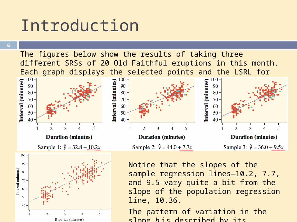
The figures below show the results of taking three different SRSs of 20 Old Faithful eruptions in this month. Each graph displays the selected points and the LSRL for that sample.

Notice that the slopes of the sample regression lines―10.2, 7.7, and 9.5―vary quite a bit from the slope of the population regression line, 10.36.

The pattern of variation in the slope b is described by its sampling distribution.

Conditions for Regression Inference

7

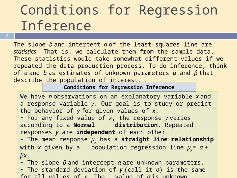
The slope b and intercept a of the least-squares line are statistics. That is, we calculate them from the sample data. These statistics would take somewhat different values if we repeated the data production process. To do inference, think of a and b as estimates of unknown parameters α and β that describe the population of interest.

We have n observations on an explanatory variable x and a response variable y. Our goal is to study or predict the behavior of y for given values of x.• For any fixed value of x, the response y varies according to a Normal

distribution. Repeated responses y are independent of each other.• The mean response µy has a straight line relationship with x given by a

population regression line µy= α + βx. • The slope β and intercept α are unknown parameters.• The standard deviation of y (call it σ) is the same for all values of x. The

value of σ is unknown.

We have n observations on an explanatory variable x and a response variable y. Our goal is to study or predict the behavior of y for given values of x.• For any fixed value of x, the response y varies according to a Normal

distribution. Repeated responses y are independent of each other.• The mean response µy has a straight line relationship with x given by a

population regression line µy= α + βx. • The slope β and intercept α are unknown parameters.• The standard deviation of y (call it σ) is the same for all values of x. The

value of σ is unknown.

Conditions for Regression InferenceConditions for Regression Inference

Conditions for Regression Inference

8

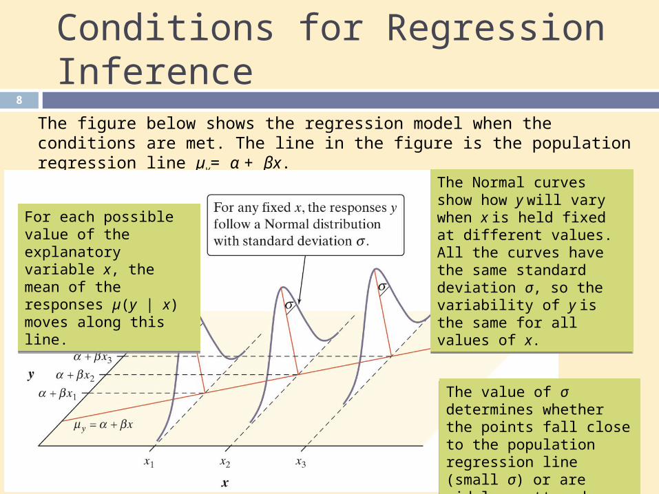
The figure below shows the regression model when the conditions are met. The line in the figure is the population regression line µy= α + βx.

The Normal curves show how y will vary when x is held fixed at different values. All the curves have the same standard deviation σ, so the variability of y is the same for all values of x.

The Normal curves show how y will vary when x is held fixed at different values. All the curves have the same standard deviation σ, so the variability of y is the same for all values of x.

The value of σ determines whether the points fall close to the population regression line (small σ) or are widely scattered (large σ).

The value of σ determines whether the points fall close to the population regression line (small σ) or are widely scattered (large σ).

For each possible value of the explanatory variable x, the mean of the responses µ(y | x) moves along this line.

For each possible value of the explanatory variable x, the mean of the responses µ(y | x) moves along this line.

Estimating the Parameters9

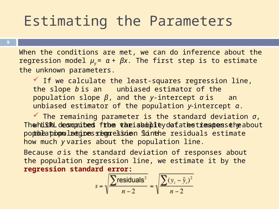
When the conditions are met, we can do inference about the regression model µy = α + βx. The first step is to estimate the unknown parameters.

If we calculate the least-squares regression line, the slope b is an unbiased estimator of the population slope β, and the y-intercept a is an unbiased estimator of the population y-intercept α. The remaining parameter is the standard deviation σ, which describes

the variability of the response y about the population regression line.

The LSRL computed from the sample data estimates the population regression line. So the residuals estimate how much y varies about the population line.

Because σ is the standard deviation of responses about the population regression line, we estimate it by the regression standard error:

10

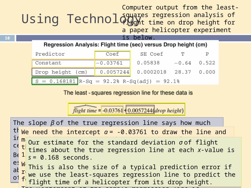
Using TechnologyComputer output from the least-squares regression analysis of flight time on drop height for a paper helicopter experiment is below.

The slope β of the true regression line says how much the average flight time of the paper helicopters increases when the drop height increases by 1 centimeter.

Because b = 0.0057244 estimates the unknown β, we estimate that, on average, flight time increases by about 0.0057244 seconds for each additional centimeter of drop height.

The slope β of the true regression line says how much the average flight time of the paper helicopters increases when the drop height increases by 1 centimeter.

Because b = 0.0057244 estimates the unknown β, we estimate that, on average, flight time increases by about 0.0057244 seconds for each additional centimeter of drop height.

We need the intercept a = -0.03761 to draw the line and make predictions, but it has no statistical meaning in this example. No helicopter was dropped from less than 150 cm, so we have no data near x = 0.

We might expect the actual y-intercept α of the true regression line to be 0 because it should take no time for a helicopter to fall no distance.

The y-intercept of the sample regression line is -0.03761, which is pretty close to 0.

We need the intercept a = -0.03761 to draw the line and make predictions, but it has no statistical meaning in this example. No helicopter was dropped from less than 150 cm, so we have no data near x = 0.

We might expect the actual y-intercept α of the true regression line to be 0 because it should take no time for a helicopter to fall no distance.

The y-intercept of the sample regression line is -0.03761, which is pretty close to 0.

Our estimate for the standard deviation σ of flight times about the true regression line at each x-value is s = 0.168 seconds.

This is also the size of a typical prediction error if we use the least-squares regression line to predict the flight time of a helicopter from its drop height.

Our estimate for the standard deviation σ of flight times about the true regression line at each x-value is s = 0.168 seconds.

This is also the size of a typical prediction error if we use the least-squares regression line to predict the flight time of a helicopter from its drop height.

11

Testing the Hypothesis of No Linear Relationship

When the conditions for inference are met, we can use the slope b of the sample regression line to construct a confidence interval for the slope β of the population (true) regression line. We can also perform a significance test to determine whether a specified value of β is plausible. The null hypothesis has the general form H0: β = hypothesized value. To do a test, standardize b to get the test statistic:

To find the P-value, use a t distribution with n - 2 degrees of freedom. Here are the details for the t test for the slope.

To test the hypothesis H0 : β = 0, compute the test statistic:

In this formula, the standard error of the least-square slope b is:

Find the P-value by calculating the probability of getting a t statistic this large or larger in the direction specified by the alternative hypothesis Ha. Use the t distribution with df = n – 2.

To test the hypothesis H0 : β = 0, compute the test statistic:

In this formula, the standard error of the least-square slope b is:

Find the P-value by calculating the probability of getting a t statistic this large or larger in the direction specified by the alternative hypothesis Ha. Use the t distribution with df = n – 2.

Significance Test for Regression SlopeSignificance Test for Regression Slope

Example12

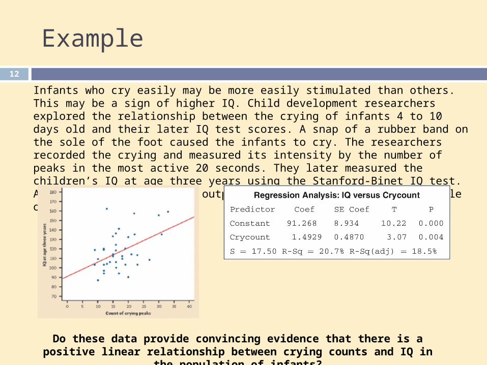
Infants who cry easily may be more easily stimulated than others. This may be a sign of higher IQ. Child development researchers explored the relationship between the crying of infants 4 to 10 days old and their later IQ test scores. A snap of a rubber band on the sole of the foot caused the infants to cry. The researchers recorded the crying and measured its intensity by the number of peaks in the most active 20 seconds. They later measured the children’s IQ at age three years using the Stanford-Binet IQ test. A scatterplot and Minitab output for the data from a random sample of 38 infants is below.

Do these data provide convincing evidence that there is a positive linear relationship between crying counts and IQ in the population of infants?

Example13

State: We want to perform a test ofH0 : β = 0 Ha : β > 0

where β is the true slope of the population regression line relating crying count to IQ score. No significance level was given, so we’ll use α = 0.05.

Plan: If the conditions are met, we will perform a t test for the slope β.

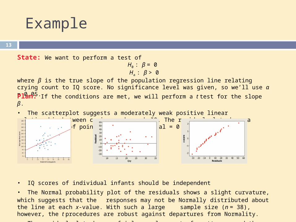
• The scatterplot suggests a moderately weak positive linear relationship between crying peaks and IQ. The residual plot shows a random scatter of points about the residual = 0 line.

• IQ scores of individual infants should be independent

• The Normal probability plot of the residuals shows a slight curvature, which suggests that the responses may not be Normally distributed about the line at each x-value. With such a large sample size (n = 38), however, the t procedures are robust against departures from Normality.

• The residual plot shows a fairly equal amount of scatter around the horizontal line at 0 for all x-values.

Example14

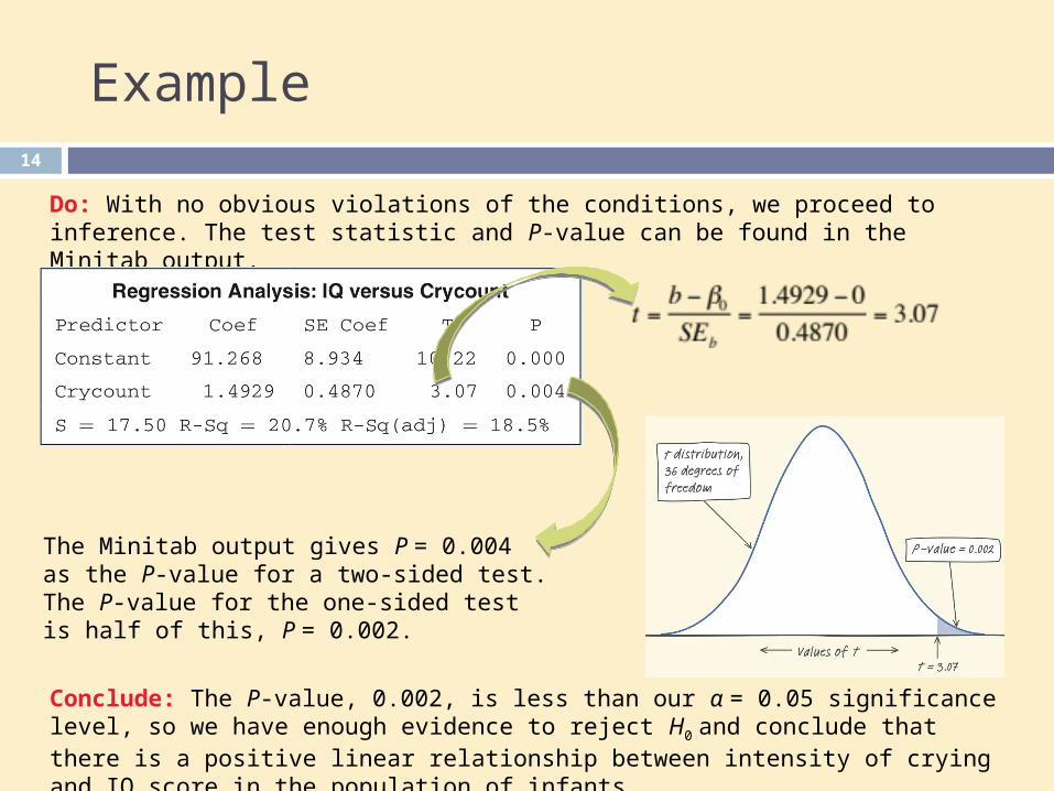
Do: With no obvious violations of the conditions, we proceed to inference. The test statistic and P-value can be found in the Minitab output.

Conclude: The P-value, 0.002, is less than our α = 0.05 significance level, so we have enough evidence to reject H0 and conclude that there is a positive linear relationship between intensity of crying and IQ score in the population of infants.

The Minitab output gives P = 0.004 as the P-value for a two-sided test. The P-value for the one-sided test is half of this, P = 0.002.

Testing Lack of Correlation15

The least-squares regression slope b is closely related to the correlation r between the explanatory and response variables. In the same way, the slope β of the population regression line is closely related to the correlation between x and y in the population.

Testing the null hypothesis H0: β = 0 is therefore exactly the same as testing that there is no correlation between x and y in the population from which we drew our data.

Testing the null hypothesis H0: β = 0 is therefore exactly the same as testing that there is no correlation between x and y in the population from which we drew our data.

Confidence Intervals for Regression Slope

16

The slope β of the population (true) regression line µy = α + βx is the rate of change of the mean response as the explanatory variable increases. We often want to estimate β. The slope b of the sample regression line is our point estimate for β. A confidence interval is more useful than the point estimate because it shows how precise the estimate b is likely to be. The confidence interval for β has the familiar form:

statistic ± (critical value) · (standard deviation of statistic)

A level C confidence interval for the slope β of the population regression line is:b ± t* SEb

Here t* is the critical value for the t distribution with df = n – 2 having area C between -t* and t*. The formula for SEb is the same as we used for the significance test.

A level C confidence interval for the slope β of the population regression line is:b ± t* SEb

Here t* is the critical value for the t distribution with df = n – 2 having area C between -t* and t*. The formula for SEb is the same as we used for the significance test.

Confidence Interval for Regression SlopeConfidence Interval for Regression Slope

Because we use the statistic b as our estimate, the confidence interval is:

b ± t* SEb

Example17

Construct and interpret a 95% confidence interval for the slope of the population regression line for the paper helicopter flight time example we referred to earlier.

SEb = 0.0002018, from the “SE Coef ” column in the computer output.

Because the conditions are met, we can calculate a t interval for the slope β based on a t distribution with df = n – 2 = 70 – 2 = 68. Using the more conservative df = 60 from Table B gives t* = 2.000.

The 95% confidence interval is:b ± t* SEb = 0.0057244 ± 2.000(0.0002018)

= 0.0057244 ± 0.0004036 = (0.0053208, 0.0061280)

We are 95% confident that the interval from 0.0053208 to 0.0061280 seconds per cm captures the slope of the true regression line relating the flight time y and drop height x of paper helicopters.

We are 95% confident that the interval from 0.0053208 to 0.0061280 seconds per cm captures the slope of the true regression line relating the flight time y and drop height x of paper helicopters.

Inference About Prediction18

One of the most common reasons to fit a line to data is to predict the response to a particular value of the explanatory variable. We want, not simply a prediction, but a prediction with a margin of error that describes how accurate the prediction is likely to be.

There are two types of predictions: predicting the mean response of all subjects with a certain value

x* of the explanatory variable predicting the individual response for one subject with a certain

value x* of the explanatory variable Predicted values are the same for each case, but the margin of error

is different.

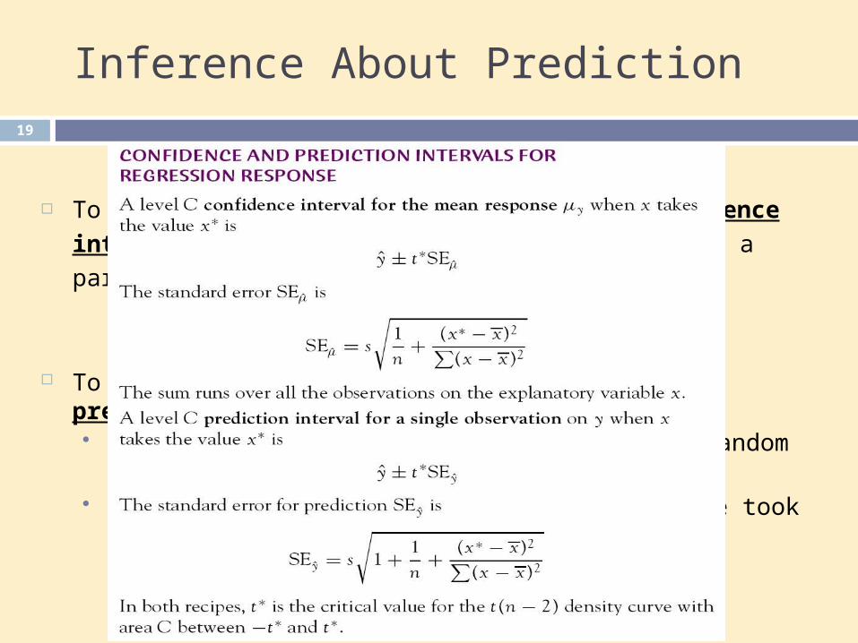
Inference About Prediction19

To estimate the mean response µy, use a confidence interval for the

parameter µy = + x*. This is a parameter, whose value we don’t

know.

To estimate an individual response y, use a prediction interval A prediction interval estimates a single random response y rather

than a parameter like µy The response y is not a fixed number. If we took more

observations with x = x*, we would get different responses.

Checking the Conditions for Inference

20

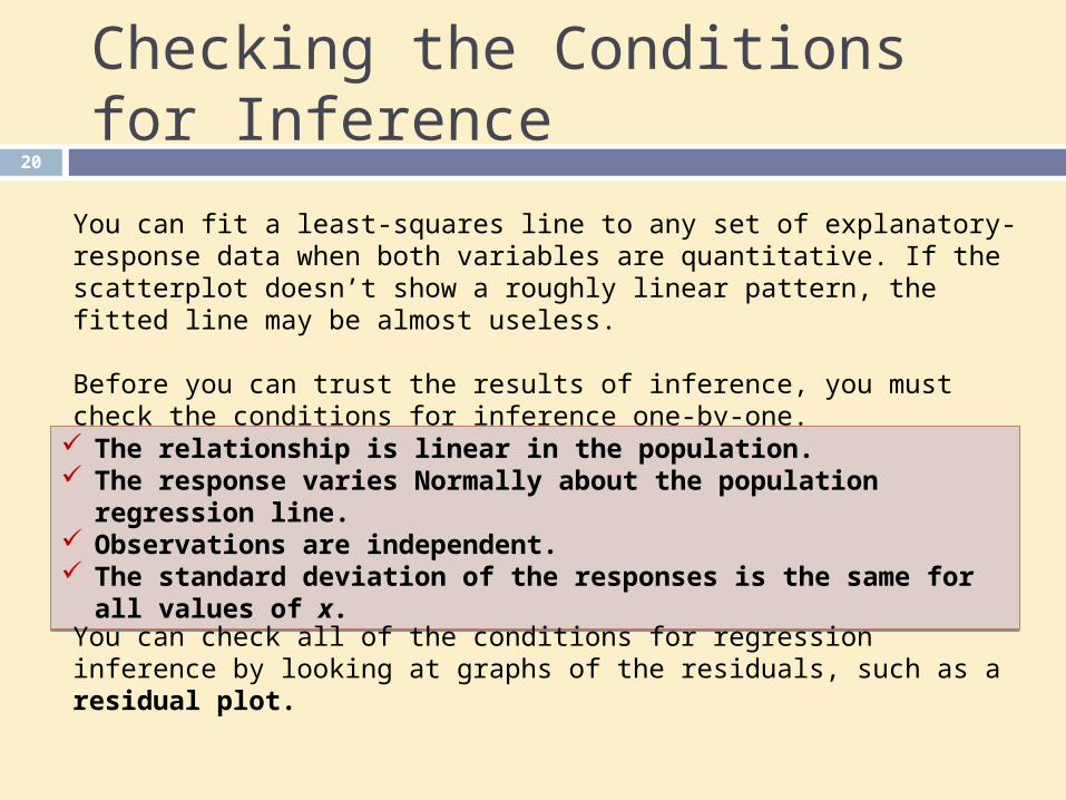
You can fit a least-squares line to any set of explanatory-response data when both variables are quantitative. If the scatterplot doesn’t show a roughly linear pattern, the fitted line may be almost useless.

Before you can trust the results of inference, you must check the conditions for inference one-by-one.

The relationship is linear in the population. The response varies Normally about the population regression line. Observations are independent. The standard deviation of the responses is the same for all values of x.

The relationship is linear in the population. The response varies Normally about the population regression line. Observations are independent. The standard deviation of the responses is the same for all values of x.

You can check all of the conditions for regression inference by looking at graphs of the residuals, such as a residual plot.

Chapter 24 Objectives Review

21

Check conditions for inference Estimate the parameters Conduct a significance test about the slope of a

regression line Conduct a significance test about correlation Construct and interpret a confidence interval

for the regression slope Perform inference about prediction