Chapter 24 Comparing Means 401...Chapter 24 Comparing Means 401 Chapter 24 – Comparing Means 1....

Chapter 24 Comparing Means 401

Chapter 24 – Comparing Means

1. Dogs and calories.

Yes, the 95% confidence interval would contain 0. The high P-value means that we lackevidence of a difference, so 0 is a possible value for µ µ

Meat Beef− .

2. Dogs and sodium.

Yes, the 95% confidence interval would contain 0. The high P-value means that we lackevidence of a difference, so 0 is a possible value for µ µ

Meat Beef− .

3. Dogs and fat.

a) Plausible values for µ µMeat Beef

− are all negative, so the mean fat content is probably higher

for beef hot dogs.

b) The fact that the confidence interval does not contain 0 indicates that the difference issignificant.

c) The corresponding alpha level is 10%.

4. Washers.

a) Plausible values for µ µTop Front

− are all negative, so the mean cycle time is probably higher

for front loading machines.

b) The fact that the confidence interval does not contain 0 indicates that the difference issignificant.

c) The corresponding alpha level is 2%.

5. Dogs and fat, second helping.

a) False. The confidence interval is about means, not about individual hot dogs.

b) False. The confidence interval is about means, not about individual hot dogs.

c) True.

d) False. Confidence intervals based on other samples will also try to estimate the truedifference in population means. There’s not reason to expect other samples to conform tothis result.

e) True.

6. Second load of wash.

a) False. The confidence interval is about means, not about individual hot dogs.

b) False. The confidence interval is about means, not about individual hot dogs.

c) False. Confidence intervals based on other samples will also try to estimate the truedifference in population means. There’s not reason to expect other samples to conform tothis result.

d) True. e) True.

Copyright 2010 Pearson Education, Inc.

402 Part VI Learning About the World

7. Learning math.

a) The margin of error of this confidence interval is (11.427 – 5.573)/2 = 2.927 points.

b) The margin of error for a 98% confidence interval would have been larger. The criticalvalue of t∗is larger for higher confidence levels. We need a wider interval to increase thelikelihood that we catch the true mean difference in test scores within our interval. In otherwords, greater confidence comes at the expense of precision.

c) We are 95% confident that the mean score for the CPMP math students will be between5.573 and 11.427 points higher on this assessment than the mean score of the traditionalstudents.

d) Since the entire interval is above 0, there is strong evidence that students who learn withCPMP will have higher mean scores is algebra than those in traditional programs.

8. Stereograms.

a) We are 90% confident that the mean time required to “fuse” the image for people whoreceive no information or verbal information only will be between 0.55 and 5.47 secondslonger than the mean time required to “fuse” the image for people who receive both verbaland visual information.

b) Since the entire interval is above 0, there is evidence that viewing the picture of the imagehelps people “see” the 3D image.

c) The margin of error for this interval is (5.47 – 0.55)/2 = 2.46 seconds.

d) 90% of all random samples of this size will produce intervals that will contain the truevalue of the mean difference between the times of the two groups.

e) A 99% confidence interval would be wider. The critical value of t∗is larger for higherconfidence levels. We need a wider interval to increase the likelihood that we catch thetrue mean difference in test scores within our interval. In other words, greater confidencecomes at the expense of precision.

f) The conclusion reached may very well change. A wider interval may contain the meandifference of 0, failing to provide evidence of a difference in mean times.

9. CPMP, again.

a) H0: The mean score of CPMP students is the same as the mean score of traditional students.µ µ µ µC T C T= − =( ) or 0

HA: The mean score of CPMP students is different from the mean score of traditionalstudents. µ µ µ µC T C T≠ − ≠( ) or 0



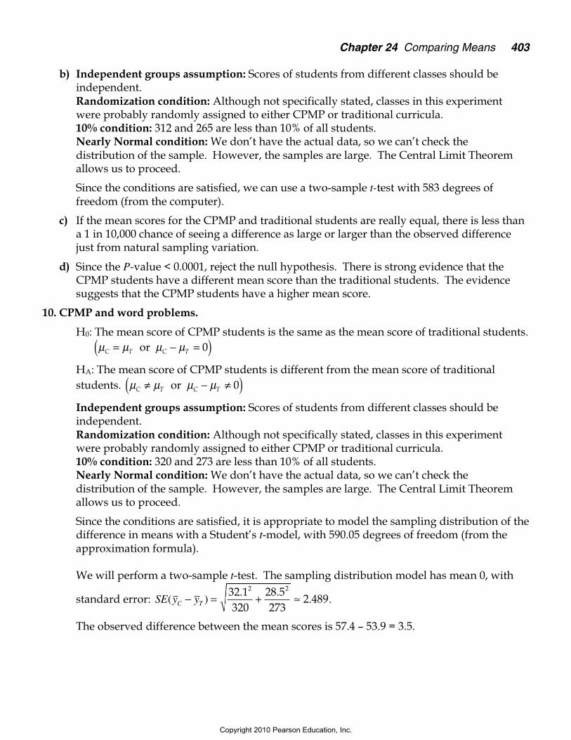
b) Independent groups assumption: Scores of students from different classes should beindependent.Randomization condition: Although not specifically stated, classes in this experimentwere probably randomly assigned to either CPMP or traditional curricula.10% condition: 312 and 265 are less than 10% of all students.Nearly Normal condition: We don’t have the actual data, so we can’t check thedistribution of the sample. However, the samples are large. The Central Limit Theoremallows us to proceed.

Since the conditions are satisfied, we can use a two-sample t-test with 583 degrees offreedom (from the computer).

c) If the mean scores for the CPMP and traditional students are really equal, there is less thana 1 in 10,000 chance of seeing a difference as large or larger than the observed differencejust from natural sampling variation.

d) Since the P-value < 0.0001, reject the null hypothesis. There is strong evidence that theCPMP students have a different mean score than the traditional students. The evidencesuggests that the CPMP students have a higher mean score.

10. CPMP and word problems.

H0: The mean score of CPMP students is the same as the mean score of traditional students.µ µ µ µC T C T= − =( ) or 0

HA: The mean score of CPMP students is different from the mean score of traditionalstudents. µ µ µ µC T C T≠ − ≠( ) or 0

Independent groups assumption: Scores of students from different classes should beindependent.Randomization condition: Although not specifically stated, classes in this experimentwere probably randomly assigned to either CPMP or traditional curricula.10% condition: 320 and 273 are less than 10% of all students.Nearly Normal condition: We don’t have the actual data, so we can’t check thedistribution of the sample. However, the samples are large. The Central Limit Theoremallows us to proceed.

Since the conditions are satisfied, it is appropriate to model the sampling distribution of thedifference in means with a Student’s t-model, with 590.05 degrees of freedom (from theapproximation formula).

We will perform a two-sample t-test. The sampling distribution model has mean 0, with

standard error: SE y yC T( ). .

.− = + ≈32 1320

28 5273

2 4892 2

.

The observed difference between the mean scores is 57.4 – 53.9 = 3.5.



Since the P-value = 0.1602, wefail to reject the nullhypothesis. There is noevidence that the CPMPstudents have a differentmean score on the wordproblems test than thetraditional students.

11. Commuting.

a) Independent groups assumption: Since the choice of route was determined at random, thecommuting times for Route A are independent of the commuting times for Route B.Randomization condition: The man randomly determined which route he would travel oneach day.Nearly Normal condition: The histograms of travel times for the routes are roughlyunimodal and symmetric. (Given)

Since the conditions are satisfied, it is appropriate to model the sampling distribution of thedifference in means with a Student’s t-model, with 33.1 degrees of freedom (from theapproximation formula). We will construct a two-sample t-interval, with 95% confidence.

( ) ( ) . , ..y y ts

n

s

ntB A df

B

B

A

A

− ± + = − ± + ≈ ( )∗ ∗2 2

33 1

2 2

43 40220

320

1 36 4 64

We are 95% confident that Route B has a mean commuting time between 1.36 and 4.64minutes longer than the mean commuting time of Route A.

b) Since 5 minutes is beyond the high end of the interval, there is no evidence that the Route Bis an average of 5 minutes longer than Route A. It appears that the old-timer may beexaggerating the average difference in commuting time.

12. Pulse rates.

a) The boxplots suggest that the mean pulse rates for men and women are roughly equal, butthat females’ pulse rates are more variable.

b) Independent groups assumption: There is no reason to believe that the pulse rates for menand women are related.Randomization condition: There is no mention of randomness, but we can assume that theresearcher chose a representative sample of men and women with regards to pulse rate.Nearly Normal condition: The boxplots are reasonably symmetric. Let’s hope thedistributions of the samples are unimodal, too.

The conditions for inference are satisfied, so we can analyze these data using the methodsdiscussed in this chapter.



c) Since the conditions are satisfied, it is appropriate to model the sampling distribution of thedifference in means with a Student’s t-model, with 40.2 degrees of freedom (from theapproximation formula). We will construct a two-sample t-interval, with 90% confidence.

( ) ( . . ). .

. , ..y y ts

n

s

ntM F df

M

M

F

F

− ± + = − ± + ≈ −( )∗ ∗2 2

40 2

2 2

72 75 72 6255 37225

287 69987

243 025 3 275

We are 90% confident that the mean pulse rate for men is between 3.025 points lower and3.275 points higher than the mean pulse rate for women.

d) Since 0 is in the interval, there is no evidence of a difference in mean pulse rate for men andwomen. This confirms our answer to part a.

13. Cereal.

Independent groups assumption: The percentage of sugar in the children’s cereals isunrelated to the percentage of sugar in adult’s cereals.Randomization condition: It is reasonable to assume that the cereals are representative ofall children’s cereals and adult cereals, in regardto sugar content.Nearly Normal condition: The histogram ofadult cereal sugar content is skewed to the right,but the sample sizes are of reasonable size. TheCentral Limit Theorem allows us to proceed.

Since the conditions are satisfied, it isappropriate to model the sampling distributionof the difference in means with a Student’s t-model, with 42 degrees of freedom (from theapproximation formula). We will construct a two-sample t-interval, with 95% confidence.

( ) ( . . ). .

. , .y y ts

n

s

ntC A df

C

C

A

A

− ± + = − ± + ≈ ( )∗ ∗2 2

42

2 2

46 8 10 15366 41838

197 61239

2832 49 40 80

We are 95% confident that children’s cereals have a mean sugar content that is between32.49% and 40.80% higher than the mean sugar content of adult cereals.

14. Egyptians.

a) Independent groups assumption: The skullbreadth of Egyptians in 4000 B.C.E isindependent of the skull breadth ofEgyptians almost 4 millennia later!Randomization condition: It is reasonable toassume that the skulls measured have skullbreadths that are representative of allEgyptians of the time.Nearly Normal condition: The histograms ofskull breadths are both unimodal and symmetric.

0 15 30

5

10

15

adult

30 45 60

2

4

6

children

127.5 135.0 142.5

2

4

6

8

200 BCE

116 128 140

2

4

6

8

10

4000 BCE



b) Since the conditions are satisfied, it is appropriate to model the sampling distribution of thedifference in means with a Student’s t-model, with 54 degrees of freedom (from theapproximation formula). We will construct a two-sample t-interval, with 95% confidence.

( ) ( . . ). .

. , .y y ts

n

s

ntK df

K

K200 4

2002

200

42

454

2 2

135 633 131 3674 03846

305 12925

301 88 6 66− ± + = − ± + ≈ ( )∗ ∗

We are 95% confident that Egyptian males in 200 B.C.E. had a mean skull breadth between1.88 and 6.66 mm larger than the mean skull breadth of Egyptian males in 4000 B.C.E.

c) Since the interval is completely above 0, there is evidence that the mean breadth of males’skulls has changed over this time period. The evidence suggests that the mean skullbreadth has increased.

15. Reading.

H0: The mean reading comprehension score of students who learn by the new method isthe same as the mean score of students who learn by traditional methods.µ µ µ µN T N T= − =( ) or 0

HA: The mean reading comprehension score of students who learn by the new method isgreater than the mean score of students who learn by traditional methods.µ µ µ µN T N T> − >( ) or 0

Independent groups assumption: Studentscores in one group should not have an impacton the scores of students in the other group.Randomization condition: Students wererandomly assigned to classes.Nearly Normal condition: The histograms of thescores are unimodal and symmetric.

Since the conditions are satisfied, it is appropriate to model the sampling distribution of thedifference in means with a Student’s t-model, with 33 degrees of freedom (from theapproximation formula). We will perform a two-sample t-test. We know:

y

s

n

N

N

N

===

51 7222

11 7062

18

.

.

y

s

n

T

T

T

===

41 8

17 4495

20

.

.

The sampling distribution model has mean 0, with standard error:

SE y yN T( ). .

.− = + ≈11 706218

17 449520

4 7792 2

.

The observed difference between the mean scores is 51.7222 – 41.8 ≈ 9.922.

0 40 80

2

4

6

8

10

Traditional

20 50 80

2

4

6

8

New



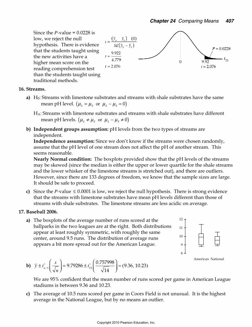
Since the P-value = 0.0228 islow, we reject the nullhypothesis. There is evidencethat the students taught usingthe new activities have ahigher mean score on thereading comprehension testthan the students taught usingtraditional methods.

16. Streams.

a) H0: Streams with limestone substrates and streams with shale substrates have the samemean pH level. µ µ µ µL S L S= − =( ) or 0

HA: Streams with limestone substrates and streams with shale substrates have differentmean pH levels. µ µ µ µL S L S≠ − ≠( ) or 0

b) Independent groups assumption: pH levels from the two types of streams areindependent.Independence assumption: Since we don’t know if the streams were chosen randomly,assume that the pH level of one stream does not affect the pH of another stream. Thisseems reasonable.Nearly Normal condition: The boxplots provided show that the pH levels of the streamsmay be skewed (since the median is either the upper or lower quartile for the shale streamsand the lower whisker of the limestone streams is stretched out), and there are outliers.However, since there are 133 degrees of freedom, we know that the sample sizes are large.It should be safe to proceed.

c) Since the P-value ≤ 0.0001 is low, we reject the null hypothesis. There is strong evidencethat the streams with limestone substrates have mean pH levels different than those ofstreams with shale substrates. The limestone streams are less acidic on average.

17. Baseball 2006.

a) The boxplots of the average number of runs scored at theballparks in the two leagues are at the right. Both distributionsappear at least roughly symmetric, with roughly the samecenter, around 9.5 runs. The distribution of average runsappears a bit more spread out for the American League.

b) y ts

nt

n±

= ±

−

∗ ∗1 139 79286

0 757998

14.

. ≈ ( . , . )9 36 10 23

We are 95% confident that the mean number of runs scored per game in American Leaguestadiums is between 9.36 and 10.23.

c) The average of 10.5 runs scored per game in Coors Field is not unusual. It is the highestaverage in the National League, but by no means an outlier.

8

9

10

11

12

American National



d) If you attempt to use two confidence intervals to assess a difference in means, you areactually adding standard deviations. But it’s the variances that add, not the standarddeviations. The two-sample difference of means procedure takes this into account.

18. Handy.

a) Males: y ts

ntM n±

= ±

≈−

∗ ∗1 4919 39

2 5250

18 67 20 11..

( . , . )

We are 95% confident that males can place between 18.67 and 20.11 pegs on average.

Females: y ts

ntF n±

= ±

≈−

∗ ∗1 4917 91

3 3950

16 95 18 87..

( . , . )

We are 95% confident that females can place between 16.95 and 18.87 pegs on average.

b) It may appear to suggest that there is no difference in the mean number of pegs placed bymales and females, but a two-sample t-interval should be constructed to assess thedifference in mean number of pegs placed.

c) ( ) ( . . ). .

. , ..y y ts

n

s

ntM F df

M

M

F

F

− ± + = − ± + ≈ ( )∗ ∗2 2

90 49

2 2

19 39 17 912 52

503 39

500 29 2 67

d) We are 95% confident that the mean number of pegs placed by males is between 0.29 and2.67 pegs higher than the mean number of pegs placed by females.

e) The two-sample t-interval is the correct procedure.

f) If you attempt to use two confidence intervals to assess a difference in means, you areactually adding standard deviations. But it’s the variances that add, not the standarddeviations. The two-sample difference of means procedure takes this into account.

19. Double header 2006.

a) ( ) ( . . )y y ts

n

s

nt

A N dfA

A

N

N

− ± + = − ±∗2 2

9 79286 9 43750 223

2 20 75799814

0 63861816

0 18 0 89∗ + ≈ −( ). .. , .

b) We are 95% confident that the mean number of runs scored in American League stadiumsis between 0.18 runs lower and 0.89 runs higher than the mean number of runs scored inNational League stadiums.

c) Since the interval contains 0, there is no evidence of a difference in the mean number ofruns scored per game in the stadiums of the two leagues.

20. Hard water.

a) H0: The mean mortality rate is the same for towns North and South of Derby.µ µ µ µN S N S= − =( ) or 0

HA: The mean mortality rate is different for towns North and South of Derby.µ µ µ µN S N S≠ − ≠( ) or 0



Independent groups assumption: The towns were sampled independently.Independence assumption: Assume that the mortality rates are in each town areindependent of the mortality rates in the others.Nearly Normal condition: We don’t have the actual data, so we can’t look at histograms ofthe distributions, but the samples are fairly large. It should be okay to proceed.

Since the conditions are satisfied, it is appropriate to model the sampling distribution of thedifference in means with a Student’s t-model, with 53.49 degrees of freedom (from theapproximation formula). We will perform a two-sample t-test.


SE y yN S( ). .

.− = + ≈138 470

34151 114

2737 546

2 2

.

The observed difference between the mean scores is1631.59 – 1388.85 = 242.74.

Since the P-value = 3 2 10 8. × − is low, we reject the nullhypothesis. There is strong evidence that the meanmortality rate different for towns north and south ofDerby. There is evidence that the mortality rate north ofDerby is higher.

b) Since there is an outlier in the data north of Derby, the conditions for inference are notsatisfied, and it is risky to use the two-sample t-test. The outlier should be removed, andthe test should be performed again. Without the actual data, we are not able to do this.The test without the outlier would probably help us reach the same conclusion, but there isno way to be sure.

21. Job satisfaction.

A two-sample t-procedure is not appropriate for these data, because the two groups are notindependent. They are before and after satisfaction scores for the same workers. Workersthat have high levels of job satisfaction before the exercise program is implemented maytend to have higher levels of job satisfaction than other workers after the program as well.

22. Summer school.

A two-sample t-procedure is not appropriate for these data, because the two groups are notindependent. They are before and after scores for the same students. Students with highscores before summer school may tend to have higher scores after summer school as well.

23. Sex and violence.

a) Since the P-value = 0.136 is high, we fail to reject the null hypothesis. There is no evidenceof a difference in the mean number of brands recalled by viewers of sexual content andviewers of violent content.

ty y

SE y y

t

t

N S

N S

=−( ) − ( )

−( )≈

≈

0

242 7437 5466 47

..

.



b) H0: The mean number of brands recalled is the same for viewers of sexual content andviewers of neutral content. µ µ µ µS N S N= − =( ) or 0

HA: The mean number of brands recalled is different for viewers of sexual content andviewers of neutral content. µ µ µ µS N S N≠ − ≠( ) or 0

Independent groups assumption: Recall of one group should not affect recall of another.Randomization condition: Subjects were randomly assigned to groups.Nearly Normal condition: The samples are large.

Since the conditions are satisfied, it is appropriate to model the sampling distribution of thedifference in means with a Student’s t-model, with 214 degrees of freedom (from theapproximation formula). We will perform a two-sample t-test.


SE y yS N( ). .

.− = + ≈1 76108

1 77108

0 242 2

.

The observed difference between the mean scores is 1.71 – 3.17 = – 1.46.

Since the P-value = 5 5 10 9. × − is low, we reject the nullhypothesis. There is strong evidence that the meannumber of brand names recalled is different for viewers ofsexual content and viewers of neutral content. Theevidence suggests that viewers of neutral ads remembermore brand names on average than viewers of sexualcontent.

24. Ad campaign.

a) We are 95% confident that the mean number of ads remembered by viewers of shows withviolent content will be between 1.6 and 0.6 lower than the mean number of brand namesremembered by viewers of shows with neutral content.

b) If they want viewers to remember their brand names, they should consider advertising onshows with neutral content, as opposed to shows with violent content.

25. Sex and violence II.

a) H0: The mean number of brands recalled is the same for viewers of violent content andviewers of neutral content. µ µ µ µV N V N= − =( ) or 0

HA: The mean number of brands recalled is different for viewers of violent content andviewers of neutral content. µ µ µ µV N V N≠ − ≠( ) or 0

Independent groups assumption: Recall of one group should not affect recall of another.Randomization condition: Subjects were randomly assigned to groups.Nearly Normal condition: The samples are large.


ty y

SE y y

t

t

S N

S N

=−( ) − ( )

−( )≈

−

≈ −

0

1 460 246 08

...




SE y yV N( ). .

.− = + ≈1 61101

1 62103

0 2262 2

.

The observed difference between the mean scores is3.02 – 4.65 = – 1.63.

Since the P-value = 1 1 10 11. × − is low, we reject the null hypothesis. There is strongevidence that the mean number of brand names recalled is different for viewers of violentcontent and viewers of neutral content. The evidence suggests that viewers of neutral adsremember more brand names on average than viewers of violent content.

b) ( ) ( . . ). .

. , ..y y ts

n

s

ntN S df

N

N

S

S

− ± + = − ± + ≈ ( )∗ ∗2 2

204 8

2 2

4 65 2 721 62103

1 85106

1 456 2 404

We are 95% confident that the mean number of brand names recalled 24 hours later isbetween 1.46 and 2.40 higher for viewers of shows with neutral content than for viewers ofshows with sexual content.

26. Ad recall.

a) He might attempt to conclude that the mean number of brand names recalled is greaterafter 24 hours.

b) The groups are not independent. They are the same people, asked at two different timeperiods.

c) A person with high recall right after the show might tend to have high recall 24 hours lateras well. Also, the first interview may have helped the people to remember the brandnames for a longer period of time than they would have otherwise.

d) Randomly assign half of the group watching that type of content to be interviewedimmediately after watching, and assign the other half to be interviewed 24 hours later.

27. Hungry?

H0: The mean number of ounces of ice cream people scoop is the same for large and smallbowls. µ µ µ µ

big small big small= − =( ) or 0

HA: The mean number of ounces of ice cream people scoop is the different for large andsmall bowls. µ µ µ µ

big small big small≠ − ≠( ) or 0

Independent groups assumption: The amount of ice cream scooped by individuals shouldbe independent.Randomization condition: Subjects were randomly assigned to groups.Nearly Normal condition: Assume that this condition is met.

ty y

SE y y

t

t

V N

V N

=−( ) − ( )

−( )≈

−

≈ −

0

1 630 2267 21

...





SE y ybig small

( ). .

.− = + ≈2 91

221 84

260 7177

2 2

oz.

The observed difference between the mean amounts is 6.58 – 5.07 = 1.51 oz.

Since the P-value of 0.0428 is low, we reject the null hypothesis. There is strong evidencethat the that the mean amount of ice cream people put into a bowl is related to the size ofthe bowl. People tend to put more ice cream into the large bowl, on average, than the smallbowl.

28. Thirsty?

H0: The mean number of milliliters of liquid people pour when asked to pour a “shot” isthe same for highballs and tumblers. µ µ µ µ

tumbler highball tumbler highball= − = or 00( )

HA: The mean number of milliliters of liquid people pour when asked to pour a “shot” isdifferent for highballs and tumblers. µ µ µ µ

tumbler highball tumbler highball≠ − ≠ or 00( )

Independent groups assumption: The amount of liquid poured by individuals should beindependent.Randomization condition: Subjects were randomly assigned to groups.Nearly Normal condition: Assume that this condition is met.



SE y ytumbler highball

( ). .

.− = + ≈17 9

9916 2

992 42

2 2

664 ml .

The observed difference between the mean amounts is60.9 – 42.2 = 18.7 ml.

ty y

SE y y

t

big small

big small

=−( ) − ( )

−( )≈

0

1 510 7

.

. 11772 104t ≈ .

ty y

SE y y

tumbler highball

tumbler highb

=−( ) − ( )

−

0

aall

t

t

( )≈

≈

18 72 42647 71

.

..



Since the P-value (less than 0.0001) is low, we reject the null hypothesis. There is strongevidence that the that the mean amount liquid people pour into a glass is related to theshape of the glass. People tend to pour more, on average, into a small, wide tumbler thaninto a tall, narrow highball glass.

29. Lower scores?

a) Assuming that the conditions for inference were met by the NAEP, a 95% confidenceinterval for the difference in mean score is:

( ) ( ) . . . , .y y ts

n

s

ndf1996 200019962

1996

20002

2000

150 147 1 960 1 22 0 61 5 39− ± + = − ± ( ) ≈ ( )∗

Since the samples sizes are very large, it should be safe to use z∗ = 1 960. for the criticalvalue of t. We are 95% confident that the mean score in 2000 was between 0.61 and 5.39points lower than the mean score in 1996. Since 0 is not contained in the interval, thisprovides evidence that the mean score has decreased from 1996 to 2000.

b) Both sample sizes are very large, which will make the standard errors of these samplesvery small. They are both likely to be very accurate. The difference in sample sizeshouldn’t make you any more certain or any less certain.

However, these results are completely dependent upon whether or not the conditions forinference were met. If, by sampling more students, the NAEP sampled from a differentpopulation, then the two years are incomparable.

30. The Internet.

a) The differences that were observed between the group of students with Internet access andthose without were too great to be attributed to natural sampling variation.

b) The researchers have incorrectly rejected their null hypothesis of no difference between thegroups, committing a Type I error.

c) There is evidence of an association between Internet access and mean science score, but thisdoes not prove that access to the Internet causes higher scores. There may be othervariables involved, such as socioeconomic status or the education level of the parents. Wewould need results from a controlled experiment to determine cause and effect.

31. Running heats.

H0: The mean time to finish is the same for heats 2 and 5. µ µ µ µ2 5 2 5 0= − =( ) or

HA: The mean time to finish is not the same for heats 2 and 5. µ µ µ µ2 5 2 5 0≠ − ≠( ) or

Independent groups assumption: The two heats were independent.Randomization condition: Runners were randomly assigned.Nearly Normal condition: The boxplots show an outlier in thedistribution of times in heat 2. We will perform the test twice, oncewith the outlier and once without. 51.25

52.50

53.75

55.00

2 5

Heat

Time





SE y y( ). .

.2 5

2 21 693197

1 200557

0 7845− = + ≈ .

The observed difference between mean times is 52.3557 – 52.3286 = 0.0271.

Since the P-value = 0.97 is high, we fail to reject the null hypothesis. Thereis no evidence that the mean time to finish differs between the two heats.

Without the outlier, it is appropriate to model the sampling distribution of the difference inmeans with a Student’s t-model, with 8.83 degrees of freedom (from the approximationformula). We will perform a two-sample t-test.


SE y y( ). .

.2 5

2 20 569556

1 200557

0 5099− = + ≈ .

The observed difference between mean times is 51.7467 – 52.3286 = –0.5819.

Since the P-value = 0.2837 ishigh, we fail to reject the nullhypothesis. There is noevidence that the mean timeto finish differs between thetwo heats.

32. Swimming heats.

H0: The mean time to finish is the same for heats 2 and 5. µ µ µ µ2 5 2 5 0= − =( ) or

HA: The mean time to finish is not the same for heats 2 and 5. µ µ µ µ2 5 2 5 0≠ − ≠( ) or

Independent groups assumption: The two heats were independent.Randomization condition: Swimmers were not randomly assigned, butif we consider these heats to be representative of seeded heats, we maybe able to generalize the results.Nearly Normal condition: The boxplots of the times in each heat showdistributions that are reasonably symmetric.

Since the conditions are satisfied, it is appropriate to model thesampling distribution of the difference in means with a Student’s t-model, with 12.62 degrees of freedom (from the approximation formula). We will performa two-sample t-test.

ty y

SE y y

t

t

=− −

−

≈

≈

( ) ( )( )

2 5

2 5

0

0 0271

0 78450 035

.

.

.

ty y

SE y y

t

t

=− −

−

≈−

≈ −

( ) ( )( )

2 5

2 5

0

0 58

0 50991 14

.

.

.

250

255

260

265

2 5

Heat

Time




SE y y( ). .

.2 5

2 23 0318

2 1498

1 3136− = + ≈ .

The observed difference between the mean times is 260.23 – 250.79 = 9.44.

Since the P-value < 0.001, we reject the null hypothesis. There is strongevidence that the mean time to finish differs between the two heats. Infact, the mean time in heat two was higher than the mean time in heat five.

33. Tees.

H0: The mean ball velocity is the same for regular and Stinger tees. µ µ µ µS R S R= − =( ) or 0

HA: The mean ball velocity is higher for the Stinger tees. µ µ µ µS R S R> − >( ) or 0

Assuming the conditions are satisfied, it is appropriate to model the sampling distributionof the difference in means with a Student’s t-model, with 7.03 degrees of freedom (from theapproximation formula). We will perform a two-sample t-test.


SE y yS R( ). .

.− = + ≈416

896

0 40002 2

.

The observed difference between the mean velocities is 128.83 – 127 = 1.83.

Since the P-value = 0.0013, we reject the null hypothesis. There is strongevidence that the mean ball velocity for stinger tees is higher than themean velocity for regular tees.

34. Golf again.

H0: The mean distance is the same for regular and Stinger tees. µ µ µ µS R S R= − =( ) or 0

HA: The mean distance is greater for the Stinger tees. µ µ µ µS R S R> − >( ) or 0

Assuming the conditions are satisfied, it is appropriate to model the sampling distributionof the difference in means with a Student’s t-model, with 9.42 degrees of freedom (from theapproximation formula). We will perform a two-sample t-test.


SE y yS R( ). .

.− = + ≈2 76

62 14

61 426

2 2

.

The observed difference between mean distances is 241 – 227.17 = 13.83.

Since the P-value <0.0001, we reject the null hypothesis. There is strongevidence that the mean distance for Stinger tees is higher than the meandistance for regular tees.

ty y

SE y y

t

t

=− −

−

≈

≈

( ) ( )( )

2 5

2 5

0

9 44

1 31367 19

.

.

.

ty y

SE y y

t

t

S R

S R

=− −

−

≈

≈

( ) ( )( )

0

1 83

0 40004 57

.

.

.

ty y

SE y y

t

t

S R

S R

=− −

−

≈

≈

( ) ( )( )

0

13 83

1 4269 70

.

.

.



35. Crossing Ontario.

a) ( ) ( . . ). .

. , ..y y ts

n

s

ntM W df

M

M

W

W

− ± + = − ± + ≈ −( )∗ ∗2 2

37 67

2 2

1196 75 1271 59304 369

20261 111

22252 89 103 21

We are 95% confident that the interval –252.89 to 103.20 minutes (–74.84 ± 178.05 minutes)contains the true difference in mean crossing times between men and women. Because theinterval includes zero, we cannot be confident that there is any difference at all.

b) Independent groups assumption: The times from the two groups are likely to beindependent of one another, provided that these were all individual swims.Randomization condition: The times are not a random sample from any identifiablepopulation, but it is likely that the times are representative of times from swimmers whomight attempt a challenge such as this. Hopefully, these times were recorded fromdifferent swimmers.Nearly Normal condition: The distributions of times are both unimodal, with no outliers.The distribution of men’s times is somewhat skewed to the left.

36. Music and memory.

a) H0: The mean memory test score is the same for those who listen to Mozart as it is for thosewho listen to rap music. µ µ µ µM R M R= − =( ) or 0

HA: The mean memory test score is greater for those who listen to Mozart than it is forthose who listen to rap music. µ µ µ µM R M R> − >( ) or 0

Independent groups assumption: The groups are not related in regards to memory score.Randomization condition: Subjects were randomly assigned to groups.Nearly Normal condition: We don’t have the actual data. We will assume that thedistributions of the populations of memory test scores are Normal.



SE y yM R( ). .

.− = + ≈3 19

203 99

291 0285

2 2

.

The observed differencebetween the mean number ofobjects remembered is10.0 – 10.72 = – 0.72.

Since the P-value = 0.7563 ishigh, we fail to reject the nullhypothesis. There is noevidence that the mean number of objects remembered by those who listen to Mozart ishigher than the mean number of objects remembered by those who listen to rap music.

ty y

SE y y

t

t

M R

M R

=− −

−

≈−

≈ −

( ) ( )( )

0

0 72

1 02850 70

.

.

.



b) ( ) ( . . ). .

. , ..y y ts

n

s

ntM N df

M

M

N

N

− ± + = − ± + ≈ − −( )∗ ∗2 2

19 09

2 2

10 0 12 773 19

204 73

135 351 0 189

We are 90% confident that the mean number of objects remembered by those who listen toMozart is between 0.189 and 5.352 objects lower than the mean of those who listened to nomusic.

37. Rap.

a) H0: The mean memory test score is the same for those who listen to rap as it is for thosewho listen to no music. µ µ µ µR N R N= − =( ) or 0

HA: The mean memory test score is lower for those who listen to rap than it is for thosewho listen to no music. µ µ µ µR N R N< − <( ) or 0

Independent groups assumption: The groups are not related in regards to memory score.Randomization condition: Subjects were randomly assigned to groups.Nearly Normal condition: We don’t have the actual data. We will assume that thedistributions of the populations of memory test scores are Normal.



SE y yR N( ). .

.− = + ≈3 9929

4 7313

1 50662 2

.

The observed differencebetween the mean number ofobjects remembered is10.72 – 12.77 = – 2.05.

Since the P-value = 0.0944 ishigh, we fail to reject the nullhypothesis. There is littleevidence that the mean number of objects remembered by those who listen to rap is lowerthan the mean number of objects remembered by those who listen to no music.

b) We did not conclude that there was a difference in the number of items remembered.

38. Cuckoos.

In order to determine whether the mean length of cuckoo eggs is the same for differentspecies, we will conduct three hypothesis tests.

Independent groups assumption: The eggs were collected from the nests of three differentspecies of bird.Randomization condition: Assume that the eggs are representative of all cuckoo eggs laidin the nest of the particular species of bird.10% condition: 14, 16, and 15 are less than 10% of all cuckoo eggs.

ty y

SE y y

t

t

R N

R N

=− −

−

≈−

≈ −

( ) ( )( )

0

2 05

1 50661 36

.

.

.



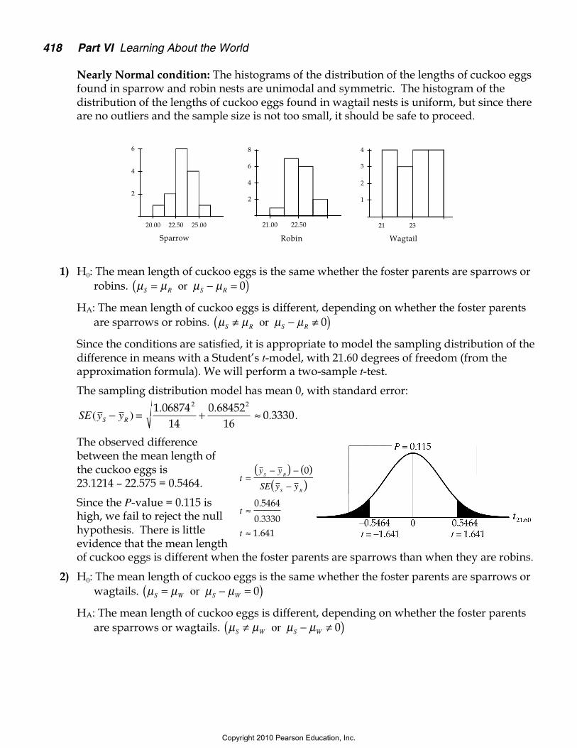
Nearly Normal condition: The histograms of the distribution of the lengths of cuckoo eggsfound in sparrow and robin nests are unimodal and symmetric. The histogram of thedistribution of the lengths of cuckoo eggs found in wagtail nests is uniform, but since thereare no outliers and the sample size is not too small, it should be safe to proceed.

1) H0: The mean length of cuckoo eggs is the same whether the foster parents are sparrows orrobins. µ µ µ µS R S R= − =( ) or 0

HA: The mean length of cuckoo eggs is different, depending on whether the foster parentsare sparrows or robins. µ µ µ µS R S R≠ − ≠( ) or 0



SE y yS R( ). .

.− = + ≈1 06874

140 68452

160 3330

2 2

.

The observed differencebetween the mean length ofthe cuckoo eggs is23.1214 – 22.575 = 0.5464.

Since the P-value = 0.115 ishigh, we fail to reject the nullhypothesis. There is littleevidence that the mean lengthof cuckoo eggs is different when the foster parents are sparrows than when they are robins.

2) H0: The mean length of cuckoo eggs is the same whether the foster parents are sparrows orwagtails. µ µ µ µS W S W= − =( ) or 0

HA: The mean length of cuckoo eggs is different, depending on whether the foster parentsare sparrows or wagtails. µ µ µ µS W S W≠ − ≠( ) or 0

21 23

1

2

3

4

Wagtail

21.00 22.50

2

4

6

8

Robin

20.00 22.50 25.00

2

4

6

Sparrow

ty y

SE y y

t

t

S R

S R

=− −

−

≈

≈

( ) ( )( )

0

0 5464

0 33301 641

.

.

.



This test is virtually identical in mechanics to the first test. We know:

y

s

n

S

S

S

===

23 1214

1 06874

14

.

.

y

s

n

W

W

W

===

22 9033

1 06762

15

.

.

t

df

P Value

==

− =

0 54926 860 587

.

.

.

Since the P-value = 0.587 is high, we fail to reject the null hypothesis. There is littleevidence that the mean length of cuckoos eggs is different when the foster parents aresparrows than when they are wagtails.

3) H0: The mean length of cuckoo eggs is the same whether the foster parents are robins orwagtails. µ µ µ µR W R W= − =( ) or 0

HA: The mean length of cuckoo eggs is different, depending on whether the foster parentsare robins or wagtails. µ µ µ µR W R W≠ − ≠( ) or 0

This test is virtually identical in mechanics to the first test. We know:

y

s

n

R

R

R

===

22 575

0 68452

16

.

.

y

s

n

W

W

W

===

22 9033

1 06762

15

.

.

t

df

P Value

= −=

− =

1 01223 600 322

.

.

.

Since the P-value = 0.322 is high, we fail to reject the null hypothesis. There is littleevidence that the mean length of cuckoo eggs is different when the foster parents arerobins than when they are wagtails.

There is no evidence to suggest a difference in mean length of cuckoo eggs that are laid inthe nests of different foster parents. In general, we should be wary of doing three t-tests onthe same data. Our Type I error is not the same for doing three tests as it is for one test.However, because none of the tests showed significant differences, this is less of a concernhere.


Chapter 24 Comparing Means 401...Chapter 24 Comparing Means 401 Chapter 24 – Comparing Means 1....

Documents

Transcript of Chapter 24 Comparing Means 401...Chapter 24 Comparing Means 401 Chapter 24 – Comparing Means 1....