Chapter 21: Correlations Between Characters

21

Correlations Between Characters

The phenotypic values of different traits in the same individualare often foundto be correlated. In humans, for example, individuals that are tall also tend to

have large feet. Such phenotypic correlations can arise from two causes.First,the expression of two characters may be modified by the same environmentalfactors operating within individuals. Some environmental factors may influenceboth characters in the samedirection,e.g., variation in resource availability duringdevelopment may influence the growthof all organs. Others may have oppositeeffects, as when an environmental cue to initiate the allocation of resources to

reproduction causes a curtailment of growth. The joint influences of all such fac-tors determine whethera within-individual environmentalcorrelation will existbetween thetraits. Such a correlation cannot be assumedto be a species-specificconstant. Just as the magnitude of the environmental variance for a trait can de-pendonthe nature of the environmentin which a population is assayed (Chapter6), so can the covariance of environmental deviations for twotraits.

Second, genetic correlations between characters can arise by two mecha-nisms. As a result of complex biochemical, developmental, and regulatory path-ways, a single gene will almost alwaysinfluence multiple traits, a phenomenonknownas pleiotropy (Wright 1968). The direction of pleiotropy may differ amonggenetic factors. Thus, at least in principle, strong pleiotropy need notresult in astrong genetic correlation between characters if the pleiotropic effects from dif-ferent loci cancel each other. A second possible source of genetic correlation isgametic phase disequilibrium between genesaffecting different characters, i.e.,the tendency of genes withlike effects on two characters to be positively or neg-atively associated in the sameindividuals. Since the pleiotropic effects of genesmay be influenced by their genetic background, and since the degree of gameticphase disequilibrium will be a function of the past history of populations, careshould also be taken in extrapolating estimates of the genetic correlation acrosspopulationsor acrosstime.

A knowledge of the mechanisms underlying the correlations between dif-ferent traits is fundamental to understanding the degree of integration of thephenotype and to resolving the constraints imposed on evolutionary processes.Depending on their sign, genetic correlations between twocharacters can eitherfacilitate or impede adaptive evolution. A conflict arises when two negatively ge-netically correlated traits are both selected in the samedirection, as the selectiveadvanceof each character tendsto pull the other character in the opposite direc-

629

630 CHAPTER 21

tion. A perfect genetic correlation between twotraits is equivalent to an absoluteevolutionary constraint, since no change in either character can occur without aparallel changein the other.

Deciphering the relative contributions of environmental and genetic factorsto phenotypic correlations is one of the most powerful and revealing applicationsof quantitative genetics. However, as we will see below, the estimation of geneticcorrelations is also an extremely demanding enterprise, requiring substantiallylarger sample sizes than are necessary in univariate analysis. For many purposes,a simple knowledge of the sign of a genetic correlation can be very revealing,and with the appropriate effort, is certainly achievable. However, as in the caseof heritability analysis, completely unambiguousestimates of the causal sourcesof covariance are not usually possible, e.g., it is generally not possible to obtaina completely unbiased estimate of the genetic correlation dueto additive geneticfactors, any more thanit is possible to obtain an absolutely clean estimate of o%by heritability analysis.

In this chapter, wefirst show how additive genetic covariances betweentraitscan be approximated by a simple extension of the methods already developedfor variance-componentanalysis of single traits. Combining these covarianceswith estimates of the additive genetic variances of the traits provides a basis forestimating the genetic correlation. Subtracting the genetic componentsof varianceand covariance at the genetic level from those at the phenotypic level yields theenvironmental components, which can thenbe usedto estimate the environmentalcorrelation. Following a consideration of issues associated with statistical analysisand hypothesis testing, we present several examples of the impact that geneticcorrelation analysis is having on evolutionary thinking.

THEORETICAL COMPOSITION OF THE GENETIC COVARIANCE

Assumingthe contribution from gametic phase disequilibrium to be negligible,Modeand Robinson (1959) showed howthe genetic covariance can be subdivided

into various components. Their workis a straightforward extension of the results

of Cockerham (1954) and Kempthorne (1954) for single characters. In order to

simplify the presentation, recall the procedure used in Chapter 5 for decomposing

the total genotypic value ofa trait influenced by twoloci. For characters 1 and 2,we have

Gi =perat lair +054 + On + 11] + [6:51 + bet]

+ [(@a)ik1 + (AQ) it+ (@Q)j6.1 + (@@)51,1]

+ [(a6d)ént1 + (06)se1,1 + (A8)ijb.1 + (a6) i511] + (Ob)ajnt +°°* (21-1a)

Go = Uc.2 + [aig + 05,2 + Ok,2 + A1,2| + [6i7,2 + Sx1,2]

+ [(aa)ik.2 + (aa)i1,2 + (aM)5,2 + (AQ)51,2]

+ [(a6)izt.2 + (6)jK1,2 + (A5)ijn.2 + (5)ig1,.2] + (66)ije1,2 +°°* (21.1b)

CORRELATIONS BETWEEN CHARACTERS 631

As in Chapter 5, a and 6 denote additive and dominanceeffects, i and 7 denotealleles at locus 1, and k and / denotealleles at locus 2. The genotypic values ofeach trait are composed of six components: the mean genotypic value for thepopulation, the total deviation from this mean dueto the additive effects of thefouralleles, the additional deviations due to the dominanceeffects at the two loci,and additive x additive, additive x dominance, and dominance x dominanceepistatic effects. Although they are written in terms of only two loci, the aboveexpressions can be generalized to any numberofloci.

Recalling that unlike terms (those having different subscripts) in Equations21.1a,b are uncorrelated under random mating and gametic phase equilibrium(Chapter 5), the genetic variances for each trait can be written as

)+o44(1) +o4p(1) toHp(1)+--- (21.2a)

(2) +05 (2) +0%44(2) +o4p(2) to%p(2)+-:- (21.2b)

= | QSN

OLN

eS + Qbs

—

The genetic covariance canalsobepartitioned into components. Using Equations21.1a,b and noting again that unlike terms are uncorrelated,

oa(1,2) = o4(1,2) + on(1,2) +o44(1,2) + capd(1,2) + opp (1,2) +--- (21.3)

where, for example,

Ja(1, 2) = o(04.1, 04,2) + 0(05,1,05.2) +0(An1, O%,2) + o(Q1.1, 012) +:°°

is the additive genetic covariance between characters 1 and 2. The second compo-nent of Equation 21.3 is attributable to the covariance of dominanceeffects, andso on for the epistatic components of variance. Note that when the twotraits arethe same, Equation 21.3 reduces to 21.2a.

In the past several chapters, numerous methodsfor the estimation of variancecomponents were covered. All of these methods are based on the sameprinciple— that the expected phenotypic covariances between various kindsof relativescan be expressedas linear functions of causal componentsof genetic, and in somecases environmental, variance. These principles extend naturally to the estimationof causal components of phenotypic covariance, exceptthat instead of comparingthe sametrait in tworelatives, two different characters are compared—one in eachrelative. The expected phenotypic covariance of character | in individual x andcharacter 2 in individual y follows naturally from the formulations of Cockerham(1954) and Kempthorne (1954):

Tale, 2y) = 20ry04(1,2) + Azyon(1, 2) + (202y)?o44(1, 2)+ 20ryAryoap(1,2) + AZ,opp(1, 2) ++ (21.4)

where ©, is the coefficient of coancestry, and A,.,is the coefficientof fraternity ofx and y (both defined as in Chapter 7). Note that when z = y, then 202, = Ary =

632 CHAPTER 21

1, and Equation 21.4 reduces to the total genetic covariance given in Equation21.3.

ESTIMATION OF THE GENETIC CORRELATION

All of the regression and ANOVAtechniques for estimating components of vari-ance reviewedin thelast four chapters extend readily to the decomposition of thecovariance betweentwotraits, as first recognized by Hazel (1943). Three of themost frequently used approacheswill be covered here.

Pairwise Comparison of Relatives

Westart with a method that is both conceptually and computationally simple,

requiring only that data are available for pairs of relatives. Suppose, for example,

that measuresoftraits 1 and 2 have been obtained for both midparents (denoted

by x) and offspring means(denoted by y). Four types of phenotypic covariances

can then be computed:trait 1 in midparents and offspring, trait 2 in midparents

and offspring, trait 1 in midparents and 2 in offspring, and vice versa. Thefirst two

of these relate to the genetic variances of the traits, the second twoto the genetic

covariance betweenthetraits. Ignoring possible contributions from commonen-

vironmentaleffects, their expected values are respectively:

o(21m.21y) = al) 1 raat) he. (21.5a)

(Zon, Z2y) = Za?) + vaal®) fee (21.5b)

a(10, ay) = SAG?) 4 TaallA) (21.5¢)

O(Zar,Z1y) = za’) + zaall,?) force (21.5d)

These expressionsare arrived at by use of Equation 21.4, after substituting the

midparent-offspring measures of relatedness, O,, = 1/4 and A,, = 0. Assum-

ing negligible epistatic effects, the sum of the “cross-covariances,” o(2Z12, Z2y) +

o(Z2x,21y), is equal to the additive genetic covariance. Each additive genetic

variance is equivalent to twice the respective within-character covariance, i.e.,

o4(1) = 20(21x, 21y). Thus, an approximation of the additive genetic correlation

based on midparent-offspring analysis is

O(Z12; 22y) + O(Zan; Z1y) (21.6a)pA =

2 O(212, Z1y) , O(220, Z2y)

Substitution of observed for expected covariances yields the estimate r4. An al-

ternative to Equation 21.6b involves the geometric (rather than arithmetic) mean


covariance,

pac

,|

Ze2ay)(222, Z1y) (21.6b)O(Z12; Z1y) ° O(Z2n, Z2y)

However, there are two reasons whythis estimatoris less desirable than Equation21.6a. First, since geometric meansare alwaysless than arithmetic means, Equa-tion 21.6b will tend to yield biased correlation estimates that are closer to zerothan those generated with Equation 21.6a. Second, if one estimate of the geneticcovariance is negative and the other positive, Equation 21.6b is undefined.

Equation 21.6a is general in that, as a first approximation, it applies to anyset of relatives with constant degrees of relationship. For example, x and y couldrepresent the two membersof a pair of dizygotic twins. Alternatively, « mightrepresent the mean of several members of a sib group and y that of the re-maining (nonoverlapping) members. The sib groups can even consist of mix-tures of half and full sibs, as is often the case in wild-caught gravid females.This generality follows from the fact that the coefficient ©,,, in the expressionsO(212,21y), O(Z22, Z2y), O(212; Zy), and (zz, Z1y) is always the same, andthere-fore cancels out in Equations 21.6a,b.

Nonetheless, the above formulation has the same kindsof uncertainties thatwe have encountered in estimatorsof heritability. First, only in the absence ofnonadditive genetic variance and commonenvironmentaleffects does Equation21.6a reduce exactly to the additive genetic correlation, 74(1, 2) / loa(1)o4(2)].Bias from dominancecanbeeliminated entirely by using relatives with Az, = 0(such asparent-offspring or half-sib pairs). The presence of epistatic genetic vari-ance and /or commonenvironmentaleffects in x and y will inflate the estimatesofthe additive genetic variances, but since covariances can be positive or negative,the same complications maybias estimates of the additive genetic covariance ineither direction. Thus, the directional effect of confounding factors on estimatesof the additive genetic correlation remains uncertain in most cases. A second

range of +1, especially when sample sizes are small.

Nested Analysis of Variance and Covariance

The nested full-sib, half-sib design provides an alternative approachto estimat-ing genetic correlations. Recall that with this design, several different femalesare mated to eachsire, and a nested analysis of variance yields estimates of theadditive genetic variances (Chapter 18). A parallel analysis can also provide anestimate of the additive genetic covariance. Analysis of covariance is identical inform to analysis of variance except that the former employs meancross-productsof the deviationsoftraits 1 and 2 rather than mean squared deviationsof individ-ual traits (Table 21.1). A lucid overview of the procedureis given by Grossmanand Gall (1968).

634 CHAPTER 21

Table 21.1 Summary of a nested analysis of covariance involving .Nsires, .\/; dams

within the ith sire, and n,; offspring within the 7th full-sib family.

Factor df Sumsof Cross-products E,(MCP)

N M;

Sires N-1 So Soni (Zi — 21) (Za; — Za) o-(1, 2) + keoa(1, 2)

a J

+k3o0,(1, 2)

_ N M;

Dams(sires) N(M — 1) Ss Soni; (Z1i5 — Z1i) (Zai9 — Zi) oe(1, 2) + kioa(l, 2)

a)

N M, Nig

Sibs (dams) T —_ NM Ss” Ss” S_(21g —_ 2115) (Zaigk — Z2i;) o-(1, 2)

a ) kJj

N M, Nig

Total T-1 Ss Ss S_ (213k — Zz) (22ijk — Zy) | o(1, 2)

ij ok

_ ¢aQ1,2) gaa, 2)

oa(l,2) op(l,2). 30aa(1,2) oap(1,2) epp(1,2)1.2) 1 CAM | ODN AAN SADA COPANO

oa(1, 2) 7 +7 4 + 16 77 8 7 46

aa(l1,2 30 p(1, 2 30 4aA(1, 2 70 1,292(1,2) ~ al yy of yy Aal in vk )

15a 1,2+ epee) op (1,2)

Note: T is the total numberof individuals in the experiment, and M the mean number

of dams/sire. For character 1, 21;;x is the observed phenotype of the kth offspring of the

jth dam matedto the ith sire, Z1;; is the mean phenotype ofthe ijth full-sib family, 21;

is the mean phenotypeofall progeny of the ith sire, and Zis the mean phenotypeofall

individuals. Similar notation is used for character 2. MCP denotes a mean cross-product,

obtained by dividing a sum of cross-products by its respective degrees of freedom. The

coefficients k, kg, and kz are defined in Table 18.3.a

Although mostnested analysesare not perfectly balanced,it is usually prefer-

able to use only individuals for which measuresof both charactersare available

in the analysis, so that estimates of both the variances and the covariance are

based on the same sample. Obviously, when a large numberof individuals are

missing one measure, this has the unfortunate side-effect of making the variance


estimates less accurate than they would be otherwise, so in extreme cases it maybe preferable to useall of the data.

The nested analysis of variance (covariance) yields nine mean squares(cross-products) — at the sire, dam, and progenylevels, for the variance of character1, the variance of character 2, and the covariance of 1 and 2. From the observedmean squares and cross-products, and the standard expressionsfor their expec-tations (Table 21.1), estimates for the sire, dam, and within-family components ofvariance and covariance can then be extracted by the method of moments(equat-ing mean squares with their expectations and solving). Recall from Chapter 18that in a univariate analysis, the sire componentof variance is equivalent to thecovarianceof paternal half sibs, thereby providing an estimate of one-fourth theadditive genetic variancefor the trait, assuming sourcesof epistatic varianceareofnegligible significance. Similarly, in an analysis of covariance, the sire componentprovides an estimate of one-fourth the additive genetic covariance between thetwotraits. Thus, letting Var(s;), Var(s2), and Cov(s,, s2) denote estimates of thesire components of variance and covariance, the genetic correlation is estimatedby

Cov(s1, 52)i——— 21.7“ Var(s1)Var(s2) (21.7)

As discussed in the previous section, this measure of the genetic correlationcan only be taken to be an approximation, since additive epistatic interactionsare potentially included in the estimates of the genetic variances and covariance.However, the reliance on paternal half sibs should minimize the complicationsthat can arise from common-environmenteffects. Like regression analysis, anal-ysis of variancecanalso yield estimates of the genetic correlation that are outsidethe rangeof true possibilities (—1,1). The likelihoodof this situation happening canbesubstantial, as Hill and Thompson(1978) have shownfor one-way (nonnested)ANOVA ofsib families. For example, if the intraclass correlations for both traitsare t = 0.0625 (assuming only additive genetic variance,this implies h? = 0.25 or0.125, depending on whether families consist of half orfull sibs), and 160 familiesof 5 sibs are analyzed, the probability of obtaining a genetic correlation orheri-tability out of boundsis only about 0.06. However,if t = 0.025 (h? = 0.10 or 0.05),with the same sample sizes, the probability of obtaining an unrealistic estimateisnearly 0.5.

In principle, as in the case of componentsofvariance, the various componentsof a genetic covariance can be extracted by comparison of the cross-covariancesbetween different types ofrelatives, e.g., full vs. half sibs in the nested design.Itwould then be possible to procure estimates of genetic correlations due to dom-inance and various formsof epistasis in addition to additive effects. However,previous chapters have amply demonstrated the difficulties in accomplishingsuch partitioning with components of genetic variance with any reasonable de-gree of accuracy. Since the sampling variance of cross-covariancesis also very high(see below), there appearsto belittle hope of a further dissection of the genetic

636 CHAPTER 21

correlation unless the numberof families sampled is in the thousands.

Regression of Family Means

Because of technical difficulties in acquiring genetic correlation estimates and intesting for their significance, a number of investigators have opted to use thecorrelation between family mean phenotypes as a surrogate for estimating pa.

Here one simply regresses the family mean phenotypeof character 1 on that ofcharacter 2, using the same individuals to compute each mean. The rationale for

such an approachis that as the size of a family increases, the sampling error of

the mean becomes diminishingly small, leaving the family mean phenotypeasan estimate of the family mean genotypic value. However,if the heritability ofeither trait is low, this approach can yield misleading results because the variances

and covariances of family meanswill be biased estimates of the additive genetic

expectations. Although we do not advocate this approach, we elaborate onit

somewhatto illustrate the interpretative difficulties that can arise.

Suppose each family consists of a group of n individuals, all related with

coefficient of coancestry © (for example, a group of paternal half-sibs), and let

Z1; be the mean phenotypeof the ith family and z1;; be the phenotypeofthe jth

memberof that family. Assuming that all of the resemblance betweenrelatives

is a consequence of additive gene action (in particular, that there are no shared

environmental effects), the expected variance among family meansfor character

1 can then be expressed as

_ 1 1 n(n — 1)o* (214) = 30 di = —o(2104) +gO(215 210k)

j=

1) 5 2 2= + [62(1) — 200%(1)] + 2604 (1) (21.8)n

where o2(1) is the phenotypic variance of the trait. The same logic gives the

expected covariance between family meansfortraits 1 and 2 as

1o(21;, 272i) = 7 loz(l, 2) — 2004(1,2)] + 20a,4(1, 2) (21.8b)

After some algebraic rearrangement, and continuing to ignore all sources of vari-

ation and covariation except those due to additive genetic effects, the correlation

of family meansis found to be

0 (21,4 22,1) (p2/Pa)_ ) _ 21.9" PA [one + 1)(one + 1) B19)o(21i) + (22,3)

where @ = 20(n—1), h? = 03(1)/02(1) and h3 = 04,(2)/02 (2) are the heritabilities

of the traits, and p, is the phenotypic correlation. The quantity in brackets defines


the factor by whichthe regression of family means deviates from the desired valuepa. The amountof bias can be seen to depend on ¢, h?, h2, and on theratio ofphenotypic to genetic correlations.

In the extremecase in whichthe heritabilities of both traits are equalto one,the genetic and phenotypic correlations are equal (as there is no environmentalvariance), and the correlation of family means provides an unbiased estimate ofthe genetic correlation, ie., p= = pA. However, such concordanceis unlikely toarise under any other circumstances. More generally, in order for the correlationbetween family meansto closely approximate the genetic correlation, both phand ¢h5 mustbe substantially larger than one and than lez /pa|. Even if the twotraits have moderately high heritabilities, the first condition requires large familysizes. Consider, for example,the situation in which bothtraits have heritabilitiesof 0.5, 50 paternalhalf sibs (20 = 0.25) are sampled per family, and the phenotypiccorrelation is five times larger than the genetic correlation. Substituting for thequantities in the brackets, wefind that the correlation of family meansinflates theestimate of the genetic correlation by

a

factor of 1.8.A perceived advantage of the family-mean approach is that p= is a true

product-momentcorrelation. Thus, unlike the other estimators described above,the correlation among family means cannot exceed +1, and its significance canbe evaluated in a straightforward manner using standardtablesofcritical valuesfor the sample correlation coefficient. However, the actual utility of this propertyseems questionable, given the uncertainty of what pz actually measures.

A more reasonablepath to estimating the genetic correlation from familymeans involves a combination of univariate ANOVA with covariance analysis,as follows. If each family is divided into two independentgroups, one used toestimate the meanofcharacter1 andthe otherfor character2, the expected covari-ance between meansis simply 2004(1,2). Assuming common family environ-mentis not a significant source of variation, there is no bias from environmentalcovariance because the two groups being compared containdifferent individuals.Combining the resultant estimate of 04(1,2) with estimates of o%,(1) and o% (2)obtained by ANOVAprovides a basis for a relatively unbiased estimate of p4.

COMPONENTSOF THE PHENOTYPIC CORRELATION

As noted in the introduction, phenotypic covariance between twotraits arisesfrom both genetic and environmental causes. We have just seen how the basicmachineryfor estimating heritabilities can be extendedto the estimationof geneticcorrelations. However, the environmental correlation, pz, can only be calculateddirectly under a very special set of circumstances. If a collection of geneticallyhomogeneousindividuals (either a highly inbred line or a single clone) is used, sothere is no genetic variance amongindividuals within the group, the phenotypicand environmental correlations are equivalent.

638 CHAPTER 21

Ordinarily, a more circuitous route to the estimation of pz is necessary. The

usual approachis to estimate the phenotypic and genetic correlationsfirst, and

to extract the environmental correlation from the algebraic relationship between

the three quantities. The phenotypic correlation between twotraits is easily ac-

quired, as it is simply the correlation of the measures ofthe twotraits in the same

individual,o~(1, 2)

,= 21.10=~ 5) 0.) oewhere o.(1) and a,(2) are the phenotypic standard deviations of the twotraits

and o,(1,2) is the covarianceoftraits 1 and 2 in the sameindividual. Therelation-

ship between the three typesofcorrelationsis fairly easily derived. Noting that

covariances are additive (Chapter 3) and assumingthat all covariance is due to

additive genetic and special environmentaleffects, o,(1,2) = o4(1,2)+o2(., 2),

where

Equation 21.10 then expandsto

po, = hihopa + per) (1 — h2)(1 — 3) (21.11)

rearrangementof which leadsto

pz —hihepa

(1 — ha)(1 — h3) eee)pp =

(An alternative derivation based on path analysis is provided in Appendix 2.)

Estimates of the environmentalcorrelation are obtained by substituting observed

for expected quantities in this expression.

The derivation of Equation 21.12 assumes zero covariance between the ge-

netic value of trait 1 in individual x and the environmental deviation oftrait 2

in relative y, and vice versa, a reasonable assumption if maternal effects can be

ruled out. This problem aside, it should also be emphasized that because Equa-

tions 21.6, 21.7, and 21.9 only provide approximations of the additive genetic

correlation, Equation 21.12 yields only an approximation of the environmental

correlation. All of the nonadditive genetic variance and covariance thatis not in-

cluded in the estimation of p4 will contribute to pz. For example, whenthe genetic

covariance is estimated by twice the covariance of offspring and midparents, the

actual composition of the excess “environmental” covariance is

A(1, 2)mee] =on(1,2)t+op(1,2+ 2o,(1,2)—|oa4(1, 2) + 5 toap(1,2)+--:


Since any of the covariance terms can be positive or negative, estimates of en-vironmental correlations can be biased in either direction by nonadditive geneaction.

Phenotypic Correlations as Surrogate Estimates of Genetic CorrelationsBecauseof the inherent difficulties in estimating additive genetic correlations,itis of great interest to know if these have a strong tendencyto reflect the moreeasily acquired phenotypic correlations in magnitude and/or sign. If this weretrue, phenotypic correlations would provide useful, and more accessible, insightinto the directionality of constraints on multivariate evolution. Moreover, be-cause phenotypic correlations can normally be estimated with a high degree ofaccuracy, while genetic correlations usually have very large standarderrors, ifthe parametric values of genetic and phenotypic correlations tended to be equal,then estimates of the phenotypic correlation could more closely approximate thetrue genetic correlation than the genetic correlation estimate itself.

It has been noticed that estimates for genetic correlations tend to slightlyexceed phenotypic correlations in absolute magnitude (Searle 1961, Kohn andAtchley 1988, Koots et al. 1994). But a broader analysis indicates that this maybe dueto biases that arise with small sample sizes. When the “effective numberof families,” Nh,h2, where N is the actual numberof families, exceeds 50 or so,

(Cheverud 1988).Broad surveys of the literature have led Cheverud (1988, 1995) and Roff

(1995, 1996) to the conclusion that pz and p,4 not only normally have the samesign, but are also of the same magnitude (Figure 21.1). The pattern appears to beparticularly clear for morphological (as opposed to life-history) characters (Roff1996, Simons and Roff 1996). Few others have been bold enough to make theassertion that p, ~ pa, and Willis et al. (1991) point out several reasons why thegenerality of such a statementshould betreated with caution. Certainly, itis still anopen question as to whether environmentalfactors thatjointly influence twotraitsoperate through the same biochemical / developmental pathwaysaspleiotropicgenetic factors, and cases do exist in which the estimates r, and r, differ in sign(Mousseau and Roff 1987) and magnitude (Hébert et al. 1994). Nevertheless, thesimilarities between existing estimates of genetic and phenotypic correlationsare striking. Becausethelatter is a function of the former, some correspondenceisexpectedjust on the basis of samplingerror, butit seems unlikely that this accountsfor the entire pattern. Further in-depth study of this fundamentally importantproblem is certainly in order.

STATISTICAL ISSUES

640 CHAPTER 21

Males Females

1.0

Environment 2

0.6 1°

oO ~)2 oO

| oO hy = oO

Environment1

Geneticcorrelation

o ooS OV

0.4

0.2 be os : une é en . a 0.2 fory f . o ae unss|ae2sa

02 00 02 04 06 08 10 -02 00 02 04 06 08 1.0

Phenotypic correlation

Figure 21.1 Comparisonof genetic vs. phenotypic correlations for pairs of mor-

phological traits in the sandcricket, Gryllus firmus. Results are given for the two

sexes, raised in two environments that varied in temperature and photoperiod.

(From Roff 1995.)

mental correlations to aid in their interpretation. For the genetic and environ-

mental correlations, the problems here are considerable. The estimators for pa

and pr generally utilize a combination of results from different applications of

ANOVAand/orregression analysis, all employing data on the sameindividuals.

The sampling properties of functionsof statistics derived from nonindependent

analyses are poorly understood.


Hypothesis Tests

Testing for a significant phenotypiccorrelation is straightforward,as it is a con-ventional product-momentcorrelation, which can be evaluated againstcriticalvalues widely available in tables in statistics texts. For genetic correlations, thesimplest option for testing the hypothesis that p4 = 0 is based onthe principlethat significant genetic covariance between twotraits implies a significant geneticcorrelation. With the pairwise-comparison method,the significance of the regres-sion of character 2 in set y on character 1 in set x, and vice versa, can be evaluatedby the standardtest for a regressionslope.

Methodsfor evaluating the significance of an environmentalcorrelation areless well developed. However, with the nearly universalavailability ofhigh-speedcomputers, a simple procedure enables simultaneoustests for all three types ofcorrelation (rz, r4, and rz). Bootstrapping and jackknifing over families (Chapter18) are being relied upon increasingly to generate empirically derived samplingdistributions of the desired statistics (Dorn and Mitchell-Olds 1991, Brodie 1993,Paulsen 1994, Roff and Preziosi 1994). For each quasisample of the data set, theestimates r, andr4 are computed directly, and then rg is obtained by use of Equa-tion 21.11. After randomly generating numeroussets of such estimates, one canconstruct confidence intervals for the three parameters from their observed sam-pling distributions. With the paired-comparison method,an alternative procedureis to randomize membersof the set y with respectto thoseof set z, evaluating theprobability (underthe null hypothesis of no correlation) of obtaining a correlationcoefficient as extremeas that observed with the true data set. A similar approachcan be appliedto the nested design, by randomizingfull-sib families with respectto sires and dams.

Finally, we note that studies of genetic correlation usually involve thesi-multaneous analysis of several characters, not just two, resulting in tables ofcorrelations betweenall possible pairs of characters. Care then needsto be takenso as not to overinterpret the significance levels attached to single correlations.For example, supposethat one were studying

a

setof N traits, none of which areactually correlated. The probability that none of the N(.N — 1)/2 observed corre-lationsis significant(at level a) is (1 — a)"'N~)/2, The probability thatat leastone correlation would appear, by chance,to be significantat the level a or smalleris one minusthis quantity. This probability can be substantial — if N — 7, thereis a 0.19 probability that at least one of the 21 correlations will spuriously appearto be significant at the P = 0.01 level, and a 0.66 probability at the a = 0.05 level.Adjusting significance tests to account for multiple comparisonsis straightfor-ward whenthe different tests involve independentdata (Rice 1989; see Chapter14). However, in the analysis of correlated characters, the nonindependenceofdata renders conventional multiple-comparison procedures invalid, and to ourknowledgenosatisfactory solution to the problem exists.

642 CHAPTER 21

Standard Errors

By Taylor expansion (Appendix 1), Reeve (1955)first obtained an expression for

the approximate large-sample variance of r4 for the single parent-offspring re-

gression, and HammondandNicholas (1972) subsequently generalized this to

includeall types of parent-offspring combinations:

Var(ra) & x Garay 4

AnEO

raB

Crea)

4 “aera Crz)°

4

ACratre)

=

(BPP)+(Crane?)

(21.13)

where A = 1 or 2 for regressions involving midparents or single parents (respec-

tively), B = [(1/h?)+(1/h3)]/2, C = 1/(hih2), N is the numberoffamilies, nis the

numberof offspring /dam in each family, and k is the numberof offspring /sire

in each family. For midparent-offspring regressions, n = k is the family size,

whereas in the regression of paternalhalf-sibs on fathers, n = 1 and k is the num-

ber of dams/sire. Reeve (1955) provides an expressionfor n for use in unbalanced

designs, and VanVleck and Henderson (1961) present an equation for the case in

which onlya single character is measured in each individual (such ascharacter 1

in parents and character 2 in offspring).

The preceding formula serves as a useful guide in choosing an adequate

experimental design.If the constraint on the investigator is the total numberof

individuals that can be measured, T = Nk, then it can be seen that Var(r4) is

minimized by maximizing the numberof families (NV). (This approach minimizes

the first term in the equation, while the remaining terms, whose denominators

are T = Nk, are unaffected.) Thus, the optimal design for estimating a genetic

correlation is to measure a single offspring from as many families as possible.

This recommendationis similar to that for heritability estimation based on parent-

offspring regression (Chapter 17).VanVleck and Henderson (1961) and Brown(1969) used simulation studies to

evaluate the degree of accuracy in using Equation 21.13 to estimate the standard

error of a genetic correlation by substituting observed for expected quantities. For

N < 100, they foundthat estimates from Equation 21.13 are biased downwards

and may underestimate the true sampling variance by as much as an orderof

magnitude with appreciable frequency. However, if N is on the orderof 1,000,

andthetrue value of r4 is not very nearly +1.0, Equation 21.13 is quite accurate.

VanVleck and Henderson (1961) and Brown (1969) also examined the sam-

pling distribution of r4. Provided geneactionis additive, Equation 21.6a appears

to yield an unbiased estimate of r4, and provided the true value p4 is not very

nearly +1.0, the sampling distribution of r4 approximates normality as sample

sizes become large. Thus, when N is large, 2,/Var(r4) usually can be taken as


PA = 0.0

|0.15

0.10

0.05

“03 -0.1 00 01 03

oO5 Pas 0.55oO PA = 0.5

= |0.20 0.20

0.15 0.15

0.10 0.10

0.05 0.05 1.0 -06 -03 0.0 03 06 1.0

Genetic correlation

Figure 21.2 Sampling distributions of the additive genetic correlation estimatedwith regression of single offspring on N single parents, using simulated datasets. In all cases, both characters have heritabilities equal to 0.4. Values of theunderlying parameters are: (A) p, = 0.0, p4 = 0.0, N = 200; (B) pz = 0.0,pA = 0.0, N = 1000; (C) pz = 0.5, p4 = 0.5, N = 200; (D) pz = 0.5,PA = 0.5, N = 1000. (From Brown 1969.)

an estimate of the 95% confidenceinterval for r4. It is clear from Figure 21.2 thatunless the numberof families analyzed is on the orderof 1,000 (for single parent-single offspring regressions), the standard error of r4 will be quite large. Cer-tainly, experiments that involve fewer than several hundred individuals shouldbe avoidedif at all possible (see also Klein 1974).

Several attempts have also been madeto obtain expressions for the large-sample variance of correlation coefficients obtained from nested full-sib, half-sibanalyses (Mode and Robinson 1959, Robertson 1959b, Tallis 1959, Scheinberg 1966,Abe 1969, Grossman 1970, Hammond and Nicholas 1972, Grossmanand Norton1974). The algebrais quite tedious, and anumberof the early papers contain errorsor are ratherrestrictive in their applicability. The most general expression, derivedby HammondandNicholas (1972), is rather complex, but can be summarized as

al a?§ b?D c7W )

Var(r;) ~ 2 ( + 4df,+2 dfj+2 df,,+2 (21.14a)€

644 CHAPTER 21

where i denotes z. A. or F depending on whichtype of correlation is being con-sidered, and df,. df,, and df,, refer to the degrees of freedom at the sire, dam, and

progeny levels. The terms S, D, and WVare of the form

Z, Zia\*? (Zo Zi9\° Z Z Z Z(F- 2) +(2- 2) +2/ 12 -) ( 12 | (21.14b)

Yi Cie Vo Cie Yi C12 Vo C2

where Z1, Zz, and Z, 2 refer to the mean squares and cross-products of characters

1 and 2 at the level of sires (when calculating S), dams (whencalculating D),

and replicates (when calculating W’). Vi, V2, and C;,2 denote the estimates of the

variances and covariances at the phenotypic, genetic, and environmentallevels,

depending upon whichcorrelation is being dealt with; these estimates are derived

by the usual route of the method of moments.Finally, the constants a, b, c, and e

depend uponthe nature of the correlation as follows:

a b C €

Phenotypic ky ke — ko ko — ky + k3(ky —_ 1) kiks

Genetic 1 —kpy/ky (ke — k1)/ky k3/4

Environmental —2 2ko/ky (ky — k2)/ky| + kz k

with the k; coefficients being defined in Table 18.3.

Robertson (1959b) and Tallis (1959) have considered the optimal design for

estimating the genetic correlation from a nested analysis of variance and covari-

ance, concluding that the design that minimizes the sampling variance of the

heritabilities also applies to the genetic correlations. Thus, the recommendations

of Chapter 18 may bereferred to.The important messageof this section is that attaining a reasonable degree

of confidence in any study of genetic correlation requires a very substantial data

base. Often, with sample sizes less than a few hundred individuals, the strongest

statement that can be made is whetherthe correlation is significantly positive or

negative. The conventional approachin regression analysis, and the one that we

focused onin the preceding paragraphs, is to take p = 0 as the null hypothesis.

For genetic studies concerned with constraints on the evolutionary process, an

alternativeis to let p.4 = £1 be the null hypothesis andto evaluateit against the

observed data using resampling procedures.

Bias Dueto Selection

Selection in the parental generation on the characters of interest or any other

characters correlated with them canlead to biased estimates of the genetic corre-

lation by altering the variances and covariancesrelative to the expectations prior

to selection (Van Vleck 1968, Robertson 1977b, Meyer and Thompson 1984). In

principle, this problem can be significant in studies of wild populations exposed


to natural selection. Here we consider how serious the bias can be and howitmight be corrected for.

Utilizing an early result of Pearson (1903), Lande and Price (1989) showedhow thebias can be eliminated under the assumptionthatthejoint distributionof the characters in parents and offspring is multivariate normal in the absenceofselection. Under those conditions, the partial regression coefficients in a multipleregression of offspring on parentcharacters are unaffected by selection, providedall of the characters underselection are actually includedin the analysis. Letting Cdenote the matrix of covariances between characters in unselected offspring andparents, and P be the phenotypic variance-covariance matrix in the unselectedparents, then Pearson’s result implies

CP7!=C,P;! (21.15a)

with the subscript s denoting matrices after selection. (Recall from Chapter 8thatpartial regression coefficients are obtained as the productof the covariancematrix involving predictor and responsevariables and the inverse ofthe variance-covariance matrix for the predictor variables.) Rearranging, the matrix of covari-ances between unselected parents and offspring can be expressed as

C=C,P7'!P (21.15b)

The genetic correlations that we wish to estimate are pA(t,j) = Ciz/./CuCj;,where C;,; denotes the elementin row i and columnj of C.

The aboverelationship showsthat the observed covariances in C, can betransformed into the desired elements of C if the phenotypic variance-covariancematrices before (P) and after (P,) selection are known.Thelatter is what we ob-serve from the sampled parents. Lande andPrice (1989) suggest that the elementsof P might be obtained from the unselected offspring (of the selected parents)since a single generationofselection rarely causes a significant alteration in thephenotypic covariance structureof populations. Obviously, this approachis pos-sible only if the forces of selection operating on the parents can be removed fromthe offspring, and no new onesare added, andif the sources of environmentalvariation contributing to P in the offspring generation can be kept the same asthose in the parental generation. Such conditions may be difficult to achieve inmany empirical settings.

As a simple example (from Lande and Price 1989)of the magnitudeof bias inthe genetic correlation that can be inducedbyselection, supposethat the varianceof the first of two characters under investigation has been reduced bya fraction kby selection such that the phenotypic variance in the observed (selected) parentsis o3(1) = (1 — k)o?(1), where o2(1) is the phenotypic variance of character 1before selection. Assumefurther that selection did not operate on anyothercor-related traits. Since the regression of character 2 on 1 accountsfor a fraction p= ofthe variance of character 2 (Equation 3.17), a changein the variance of character 1

646 CHAPTER 21

Expected

py

k (Fractional changein varianceoftrait 1)

Figure 21.3 Bias in the expected genetic correlation between two characters

whenthe phenotypic variance of character | in the parents has been modified

to (1 — k)o2(1) but has been unaccountedfor in the analysis. Solid circles: cor-

relation based on covariance of offspring character 2 on parent character 1; open

squares: correlation based on covariance of offspring character 1 on parent charac-

ter 2; solid line: average. Left: h? = 0.3, h3 = 0.7. Right: hj = 0.7, h2 = 0.3.

The true value p4 is 0.5 in both examples. (From Lande andPrice 1989.)

equal to —ko?(1) must induce a change in the variance of character 2 equal to

—kp2o2(2). Therefore, the phenotypic variance for character 2 in the parents after

selection is ¢2(2) = (1 — kp2)o2(2). From Pearson’sresult, we knowthatselection

does not change the regression coefficient, so if selection reduces the phenotypic

variance of character 1 by the factor k, it must reduce the phenotypic covariance

by the samefactor, i.e, 75(1,2) = (1 — k)o.(1, 2). Substituting these quantities

into P, and solving C, = CP~'P,, we obtain the expected covariances between

parents (p) and offspring (0) after selection,

o4(Z10.21p) = val) (1 —k) (21.16a)

7, (220, 22p) = va?) ( - ‘pagel (21.16b)

o4(Z10;Z2p) = za'.?) 0 ~a (21.16c)

O5(Z20;Z1p) = 2a) — k) (21.16d)


These expressionsillustrate several important points about estimates of ge-netic correlations in selected populations (Figure 21.3). First, selection that causesa change in the phenotypic varianceof the parents will usually induce changesin all four of the covariances between parents andoffspring.

Second, selection causes the two covariances between characters 1 and 2 tobe unequal, i.e., o5(210, Z2p) F Os(2Z1p, 220). In somecases, especially when theheritability of the unselected trait is relatively low, the two measures of geneticcovariance may actually differ in sign; this requires that phi /(pah2) > 1/k. Inprinciple, this property could provide a way of assessing whetherselection hascaused a significant bias in the parent sample, provided maternaleffects can beruled out. However,in light of the difficulties in procuring accurate estimates ofcovariances, sucha test is not likely to be very powerful. In general, averaging thetwo types of covariances (Equations 21.16c and d) does not improvethesituationmuch, since both are often biased in the samedirection (Figure 21.3).

Third, in extreme cases, the expected valueof the genetic correlation, as definedby Equation 21.6a, can exceedits theoreticallimits of +1 (Figure 21.3). Combiningthis problem withthe substantial sampling varianceof genetic correlations, wildlyunrealistic genetic correlations are possible with selected populations.

If any generalization can be drawn from theseresults, it is that the directionand magnitude of selection bias on the estimation of p,4 is difficult to assess inthe absenceof prior information on the composite parameter kph, /h2 and on p,4itself. (The situation is worse, of course,if selection is acting on bothtraits and/oron additionalcorrelatedtraits.) Clearly, in situations where selectionis likely tobe a problem, application of Equation 21.15b priorto analysisis highly desirable.

The mostfeasible way to eliminate selection bias is to assay the study pop-ulation in a highly protective environment, but this approach raises another fun-damentalissue. If the characters under investigation are sensitive to genotype xenvironmentinteraction (Chapter 22), then a change in environment may inducea real shift in 4, so that one is no longer estimating the correlation of inter-est. Simons and Roff (1996) found that patterns of genetic correlations amongmorphological charactersin crickets are essentially the same when estimated inconstant laboratory vs. variable field conditions, although the correspondenceamong correlations involvinglife-history traits is less pronounced. On the otherhand, Gebhardt and Stearns (1988) found that the genetic correlation betweendevelopment time and weightat eclosion in Drosophila mercatorum changed signfrom one environment to another. This issue is of special concern when oneismost interested in quantifying genetic constraints in harsh environments, whereselective mortality may be quite high and genetic constraints may play their mostimportant role. Clearly, more work is needed on the degree to which geneticcorrelations (and covariances) respond to environmental changes.

648 CHAPTER 21

APPLICATIONS

These warnings are not meantto be totally discouraging. Studies that are appro-

priately designed and meetwith the appropriate precautionscanyield substantial

insight into the constraints on the evolution of multivariate phenotypes. The fol-

lowing examples will providea feeling for the diversity of problems that can be

evaluated with a genetic covariance analysis.

Genetic Basis of Population Differentiation

Ecologists are well aware that different populations of the same species often

exhibit rather different diets. To a large extent this may simplyreflect shifts in the

relative availabilities of prey types in different areas. An alternative possibility is

the existence of genetic differences in feeding behavior. Arnold (1981a-c) studied

this issue in garter snakes (Thamnophis). In California, coastal populationsof this

snake are primarily terrestrial predators of slugs, while inland populations prey

more exclusively on fish and amphibians. A dietary shift between these two areas

is clearly necessary, since slugs are absent from inland habitats. Arnold made

several observations that were consistent with genetic differences in the feeding

habits of coastal and inland snakes. For example, about 75% of naive, newborn

snakes from the coast would attack slugs in laboratory experiments, while only

about 35% of the inland snakes would doso. The slug-refusing individuals were

quite persistent in their decision, starving to death unless alternate prey were

offered.A standard laboratory test was devised to evaluate whether the divergence

in prey preference was dueto genetic differences in chemoreceptive responses.

Cotton swabs wereeither rubbed on different prey or soaked in their extracts

and presented to naive, newborn snakes. The number of tongue flicks /minute

was then taken to be a measure of chemoreceptive response. As expected, the

coastal population was much morereceptive to slugs (Table 21.2). On the other

hand, the inland population was not significantly more responsive to fish and

amphibianodors than wasthe coastal population. Furthermore, the coastal snakes

exhibited a much stronger responseto leeches than did the inland snakes. This

latter point was surprising, since leeches are unknownin the diets of coastal

snakes.Someinsight into these results was provided by a genetic analysis of full-

sib families obtained from field-collected gravid females (19 females with

a

total

of 211 young in the inland population and 20 females with 102 young from the

coast). Becauseof the full-sib design, the genetic variances and covariances may

be biased by the presence of dominance, but common environmental effects were

ruled out on the basis of prior experiments. Estimates for the heritabilities of

chemoreceptive responsesare given in Table 21.2 and for the genetic correlations

in Table 21.3.


Table 21.2 A comparison of chemoreceptive responses to prey odors by newborn gartersnakes, Thamnophis elegans, from coastal and inland California.

Mean Tongue-flick Rate Heritability

Coast Inland Difference Coast Inland

Slugs 30.9 4.3 1.72 0.2 0.2Leeches 11.8 2.5 1.24 0.6 0.3Salamanders 9.0 7.4 0.21 0.4 0.2Frogs and tadpoles 30.5 29.8 0.17 0.4 0.3Control 1.4 1.6 —0.26 0.0 0.1

Source: Arnold (1981a,c).Note: The difference between population mean phenotypesis in units of standard devia-tions of In-transformedvalues.

The estimated genetic correlation between responsesto leeches andslugsis0.9 for both populations. Thus, any evolutionary changein oneof these responsesis expected to cause a similar shift in the other throughpleiotropy. This result helpsexplain the increase in receptivity to leeches for the coastal population, which hasevolved in the direction of slug specialization. Arnold further suggests that thedichotomy between the two populations may be magnified by an evolutionaryreduction in receptivity to leeches in the inland population. There is no positiveselection for slug predation in this population because there are no slugs. Thereare leeches, however, and their consumption maybe deleterious, since they oftenpass throughthe snake’s gut alive, causing some damagein the process.

Table 21.3. A comparisonof the genetic correlations for chemoreceptive responsesto preyodorsin coastal (above diagonal) and inland (below diagonal) populations of Thamnophiselegans.

SSeS

Sl Le Sa Fr Co

Slugs — 0.9 1.0 0.9 0.0Leeches 0.9 — 0.8 0.9 0.2Salamanders 0.5 0.8 — 0.9 0.6Frogs and tadpoles 0.6 0.4 0.2 — 0.2Controls -0.4 0.0 0.3 -0.3 —eTSource: Arnold (1981b).Note: Standard errors of the estimates are on the orderof 0.3. S] = slugs, Le = leeches, Sa= salamanders, Fr = frogs and tadpoles, and Co = control.eee

650 CHAPTER 21

If the hypothesized selective pressures due to slugs and leechesare correct,

then the similarities in responses to salamandersandfrogs in the two populationscan also be clarified. In the coastal population, chemoreceptive responsesto slugs,salamanders, and frogs are almost perfectly genetically correlated so the relativelystrong response to vertebrates may be largely a pleiotropic effect of selectionfor predation on slugs. The responses to leeches, salamanders, and frogs havelower, butstill positive, genetic correlations in the inland population. Thus, anantagonism would exist between positive selection for predation on vertebratesand selection for avoidance of leeches.

This kind of reasoning would not have been reached had Arnoldrelied solelyon phenotypic correlations. The phenotypic correlations between the variouschemoreceptive responses were uniformly low in both populations, < 0.3 in allbut one case.

The Homogeneity of Genetic Covariance Matrices Among Species

Asnotedin the previous example, characters evolve in responseto natural selec-

tion as a direct consequenceofthe forces of selection operating on the characters

themselves and as an indirect consequence of selection operating on all geneti-

cally correlated traits (see Chapter 8). Thus, any attempt to project the long-termconsequencesof selection on specific characters is highly dependenton the degree

of constancyof the genetic covariances over time. Such constancyis also required

if much progress is to be madein retrospective evaluations of the evolutionary

forces that may be responsible for observed changes in the fossil record (Reyment

1991). One approachto evaluatingthe stability of the genetic covariance matrix is

to perform temporal surveys of genetic variances and covariancesin individual

populations. But such comparisons cannot usually be made on very long time

scales. An alternative is to compare the genetic covariance structure of isolated

populationsor species. Similarity in this case would be consistent with long-term

stability.Lofsvold (1986) used the latter approach in an analysis of skull morphology

in the white-footed mouse (Peromyscus leucopus) and two subspecies of the deer

mouse(P. maniculatus bairdii and P. m. nebrascensis). The specimens were obtained

from a museum collection of preserved skulls obtained from full-sib families of

wild-caught individuals bred in the laboratory of L. R. Dice in the 1930s. Fif-

teen cranial characters were measured with calipers. After adjusting for sexual

dimorphism (Chapter 24), the additive genetic variances and covariances were

estimated from regressions of offspring means on paternal phenotype. Lofsvold

used three approaches to compare the genetic covariance matrices. Two of these

are explained relatively easily, while the third requires a rather advanced under-

standing of multivariate statistics and will not be considered here.

The first approach wasto treat the corresponding elements of two genetic

covariance matrices as paired observations and compute the ordinary correlation

coefficient, rj,, between them. An rj, equal to 1.0 would then indicate perfect pro-


portionality between the two matrices, while rjz = 0.0 would indicate a completelack of correspondence.Thisis not a test of the absolute equality of two matrices,since ray = 1.0 wouldarise if one matrix were simply a product of the second anda constant. Moreover, since thestatistical distribution of rj, is unknown,it is notpossible to attach any degree of confidence to ray.

Lofsvold’s second approach eliminates these difficulties, but in a rather arbi-trary fashion. An index of similarity, y, was computed by taking the sum of thecross-products of the corresponding elements of the two genetic covariance matri-ces being compared.The off-diagonal elements of one matrix were then randomlyrearranged by rows, and anew index computed for the randomized matrix and theother, unaltered, matrix. The randomization procedure was repeated manytimes,yielding an empirical distribution of ~ for randomly constructed matrices. Thesignificance of the observed was then determined from the cumulative distribu-tion of the randomly generated valuesof 7. For example, if a randomly generated7 greater than the observed7 arose at a frequencyless than 5%, the hypothesisthatthe observed similarity is no greater than that expected by chance wasrejectedat the 0.05 level. Although this and other procedures involving the permutationof matrix elements have been used frequently to compare variance / covariancestructures, the statistical and biological justification for their use has not beenestablished.

The three different approaches taken in this study yielded essentially thesame conclusions. While the genetic covariance structures for the two P. manicu-latus subspecies were similar (proportionally), comparisons between P. leucopusand P. maniculatus indicated pronounced differences. Thus, for this genus, theassumption of constant genetic covariance structure cannot be extended beyondthe species level. The potential response of one Peromyscus species to selectioncannot be extrapolated from information on the genetic covariance of another.

Several other attempts have been madeto test the hypothesis that closelyrelated populations or taxa have similar genetic covariance and/orcorrelationmatrices (Cheverud 1988, 1989; Kohn and Atchley 1988; Cheverud et al. 1989;Venable and Burquez 1990; Wilkinson et al. 1990; Spitze et al. 1991; Platenkampand Shaw 1992; Brodie 1993; Paulsen 1994), most of them failing to detect sig-nificant differences, probably because of low statistical power. Manystatisticsbeyond those mentioned above have been employedin these studies, e.g., thesum of squared differences between like elements, the difference between matrixdeterminants or between dominanteigenvalues, and the correlation between theelements of the leading eigenvectors. Thestatistical properties of most of thesetests are poorly understood, if not completely unknown (Cowley and Atchley1992, Shaw 1992). Consequently, most investigators apply severaldifferent tech-niquesto their data in hopes that a consistent message will emerge, and that hasusually been the case. However, such results may be

a

bit misleading, since thedifferent methodsare clearly not independent.

Prior to the application of any test for covariance matrix similarity, a funda-

652 CHAPTER 21

mentalissue that needsto be dealt with is measurementscale. If there is an asso-ciation between meansandvariances, two taxa can exhibit different covariance

structures simply because they differ in mean phenotypes. Methods for dealingwith this type of problem have been covered in Chapter 11. An equally seriousissue is the fact that different characters are often measured on fundamentallydifferent scales (e.g., length vs. volume). Without some kind of transformation,the contributions of different characters to matrix similarity indices will dependon the different measurementscales. The problem cannotbe eliminated by simplystandardizingall characters to have equal variances, since that would be contraryto the goal of the analysis. Spitze et al. (1991) suggest that each scale of measure-ment be transformed such that the variance of all characters measured on thatscale averages to one across populations. This approach has the effect of stan-

dardizing different scales with respect to each other, while preserving differencesin variance amongcharacters within and between populations.

Resampling procedures (Chapter 16) seem to provide a reasonable alternativemeansfor the comparison of covariance matrices (Spitze et al. 1991). Once the datahave been transformed, the information from both populations can be pooledinto one synthetic population. Then two quasipopulations can be constructed by

randomlyselecting families from the synthetic population, and allocating them

such that the two quasipopulations have the same number of families as the

true population samples. This procedure is repeated a thousandorso times, and

the similarity index of interest is computed for each pair of quasipopulations,

generating a null distribution of the statistic against which the observed valuefor

the true populationsis tested. One can then evaluate whether the observed valueis significantly greater than (or less than) what would be obtained by drawing

two samples from a commonpopulation. In addition to making no assumptions

aboutthe distribution of phenotypes, this bootstrap procedure has the advantage

of applying to any similarity index.If one is willing to assume that the characters under consideration have a

multivariate normal distribution, a maximum likelihood method is available for

testing the hypothesis that any element (or group of elements) of the covariance

matrices differ between two populations (Shaw 1991). Unfortunately, simulations

have shownthe powerofthis test to be quite low. For example, considering only

the univariate case, if the additive genetic variances in two populations differ by

a factor of 2.5, a nested sib analysis involving 100 sires/ population, 3 dams/sire,

and 3 offspring /dam would detect the difference at the 0.05 level of significance

only about 50% of the time. With the same design butonly 40sires, the difference

would go undetected 80% of the time. Such results should not be too surprising.

We have seen repeatedly that the procurementof accurate variance / covariance

estimates demandslarge sample sizes; detecting a significant difference between

two separate estimates can only be moredifficult. It remains to be seen whether


Logbr

ainwe

ight

Log body weight

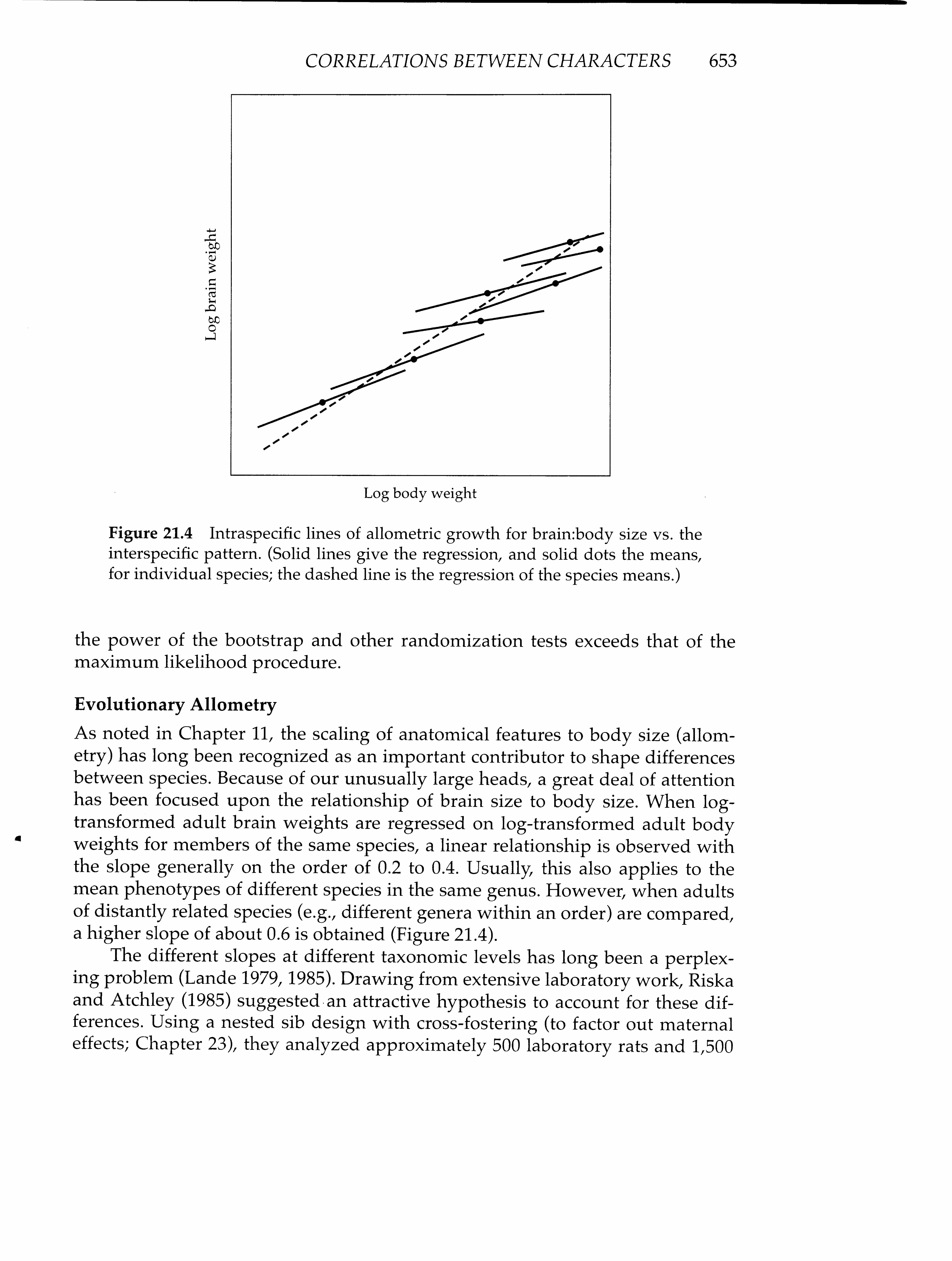
Figure 21.4 Intraspecific lines of allometric growth for brain:body size vs. theinterspecific pattern. (Solid lines give the regression, and solid dots the means,for individual species; the dashedline is the regression of the species means.)

the power of the bootstrap and other randomization tests exceeds that of themaximum likelihood procedure.

Evolutionary Allometry

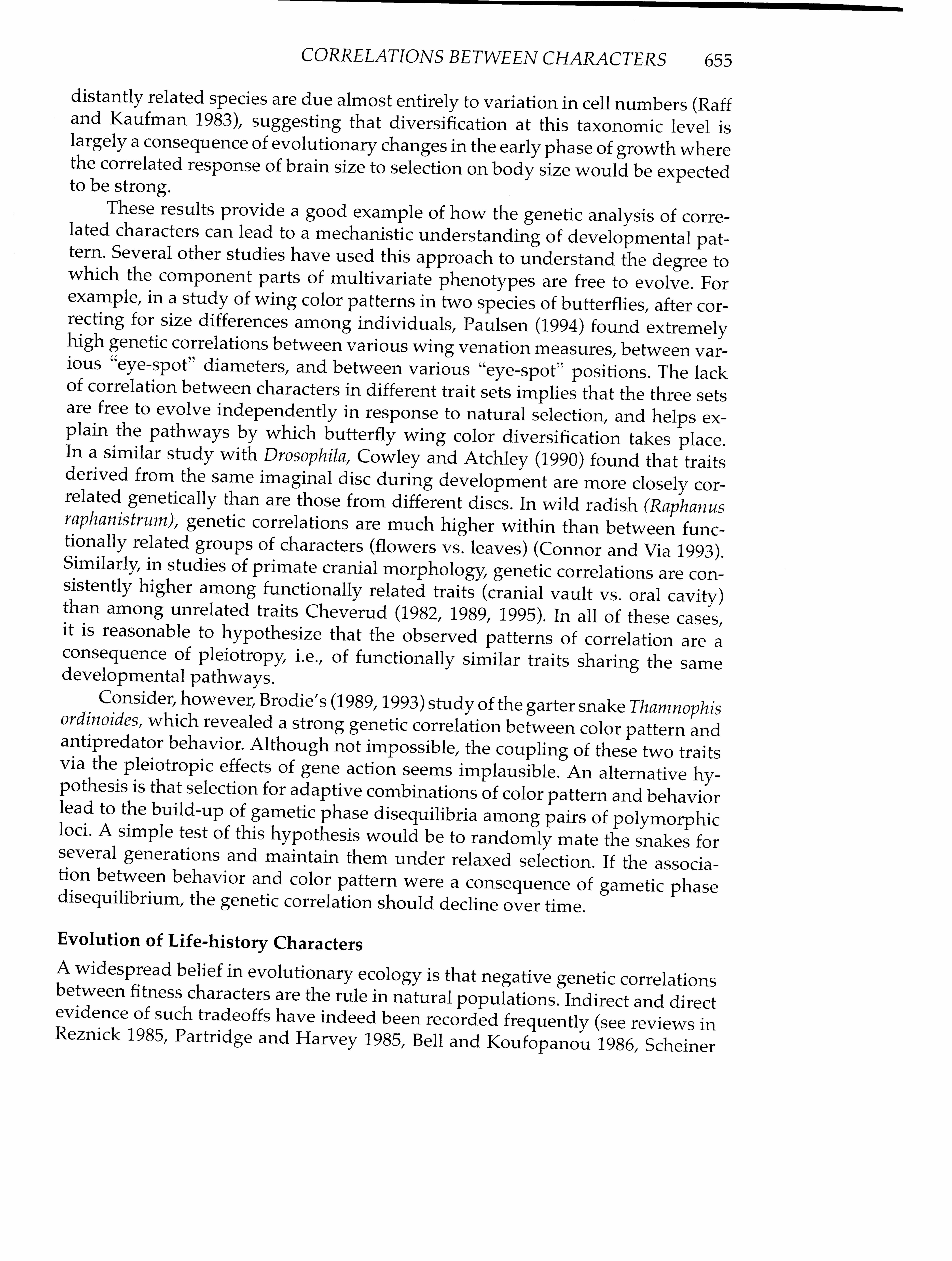
As noted in Chapter 11, the scaling of anatomical features to body size (allom-etry) has long been recognized as an important contributor to shape differencesbetweenspecies. Because of our unusually large heads, a great deal of attentionhas been focused upon the relationship of brain size to body size. When log-transformed adult brain weights are regressed on log-transformed adult bodyweights for members of the samespecies, a linear relationship is observed withthe slope generally on the order of 0.2 to 0.4. Usually, this also applies to themean phenotypesof different species in the same genus. However, when adultsof distantly related species (e.g., different genera within an order) are compared,a higher slope of about 0.6 is obtained (Figure 21.4).

The different slopes at different taxonomic levels has long been a perplex-ing problem (Lande 1979, 1985). Drawing from extensive laboratory work, Riskaand Atchley (1985) suggested.an attractive hypothesis to account for these dif-ferences. Using a nested sib design with cross-fostering (to factor out maternaleffects; Chapter 23), they analyzed approximately 500 laboratory rats and 1,500

654 CHAPTER 21

0.8

Geneticcorrelation

© ws

0 40 80 120 160 200

Age (days)

Figure 21.5 Reduction with age of the genetic correlation between final adultbrain and age-specific body weights. (From Riska and Atchley 1985.)

mice (Atchley and Rutledge 1980, Atchley et al. 1984). The experimental designprovided estimates of the genetic correlations betweenbrain size, body size, andbody growth during different age intervals. In both species, the correlation be-tween eventual adult brain weight and age-specific body weight declines withage (Figure 21.5). This reduction was found to be dueto an increasingly negativecorrelation between brain weight and growth incrementlate in life. Thus, thepositive genetic correlation between brain and bodysize is primarily a functionof genes that are active in prenatal and early postnatal growth.

Riska and Atchley pointed out that mammalian growth canbe partitionedroughly into an early phase in which cell numbers of most organsare increasingand a late phase in which cell numbers are nearly constant but cell sizes areincreasing in different organsto different degrees. Thus, genesthat influence early

growth have general pleiotropic effects on the size of most organs, while thoseoperating later in life have morespecific targets.In artificial selection experimentsfor bodysize in mice, a large proportion of the response is due to changesin cell

size (Falconeret al. 1978), indicating that late-acting genes with relatively mildpleiotropic effects are selected upon. Based on the pattern in Figure 21.5, such

selection would be expected to yield a relatively mild change in brain weight,as observed in intraspecific studies. In contrast, body size differences between

|


distantly related species are due almost entirely to variation in cell numbers(Raffand Kaufman 1983), suggesting that diversification at this taxonomic level islargely a consequenceof evolutionary changesin the early phase of growth wherethe correlated responseof brainsize to selection on body size would be expectedto be strong. |

These results provide a good example of how the genetic analysis of corre-lated characters can lead to a mechanistic understanding of developmentalpat-tern. Several other studies have used this approach to understandthe degree towhich the componentparts of multivariate phenotypes are free to evolve. Forexample, in a study of wing color patterns in two species of butterflies, after cor-recting for size differences amongindividuals, Paulsen (1994) found extremelyhigh genetic correlations between various wing venation measures, between var-ious “eye-spot” diameters, and between various “eye-spot” positions. The lackof correlation between characters in different trait sets implies that the three setsare free to evolve independently in response to natural selection, and helps ex-plain the pathways by which butterfly wing color diversification takes place.In a similar study with Drosophila, Cowley and Atchley (1990) foundthattraitsderived from the same imaginaldisc during developmentare more closely cor-related genetically than are those from different discs. In wild radish (Raphanusraphanistrum), genetic correlations are much higher within than between func-tionally related groups ofcharacters(flowers vs. leaves) (Connor and Via 1993).Similarly, in studies of primate cranial morphology, genetic correlations are con-sistently higher among functionally related traits (cranial vault vs. oral cavity)than among unrelated traits Cheverud (1982, 1989, 1995). In all of these cases,it is reasonable to hypothesize that the observed patterns of correlation are aconsequence of pleiotropy, i.e., of functionally similar traits sharing the samedevelopmental pathways.

Consider, however, Brodie’s (1989, 1993) study of the garter snake Thamnophisordinoides, whichrevealed a strong genetic correlation between color pattern andantipredator behavior. Although not impossible, the coupling of these twotraitsvia the pleiotropic effects of gene action seems implausible. An alternative hy-pothesisis that selection for adaptive combinationsof color pattern and behaviorlead to the build-up of gametic phase disequilibria amongpairs of polymorphicloci. A simple test of this hypothesis would be to randomly mate the snakes forseveral generations and maintain them underrelaxed selection. If the associa-tion between behavior and color pattern were a consequence of gametic phasedisequilibrium, the genetic correlation should decline over time.

Evolution of Life-history Characters

A widespreadbelief in evolutionary ecology is that negative genetic correlationsbetweenfitness charactersare the rule in natural populations. Indirect and directevidenceof such tradeoffs have indeed been recorded frequently (see reviewsinReznick 1985, Partridge and Harvey 1985, Bell and Koufopanou 1986, Scheiner

656 CHAPTER 21

et al. 1989), but a numberofclear cases of positive genetic correlations have also

been reported(e.g., Giesel and Zettler 1980, Hegmann and Dingle 1982, Mitchell-

Olds 1986, Rausher and Simms1989, Spitze et al. 1991). Ina broad review of the

literature, Roff (1996) found that genetic correlations between fitness characters

tend to be lower than those between morphological characters. However, there

is a broad degree ofoverlap in the distributions, and the majority of life-history

correlationsarestill positive.

Positive genetic correlations between fitness characters can be artifactual

(Rose 1984, Service and Rose 1985, Clark 1987) — a consequence of using in-

bred lines, some of which suffer from inbreeding depression more than others,

or of performing assays in a novel laboratory environmentto which populations

are not adapted. Butnotall of the data seem to be explained so easily.

The usual argumentfor the negative correlation hypothesis is that alleles

that simultaneously improve severaltraits tend to be advanced rapidly by selec-

tion, while those with several negative effects tend to be eliminated (Falconer and

Mackay 1996, Rose 1982). Such a sorting processis expected to leave circulating a

pool of alleles with favorable effects on some fitness traits but unfavorableeffects

on others,i.e., a set of alleles with equivalent effects on total fitness. Curtsinger

et al. (1994) have cast doubt upon this seductively simple hypothesis, pointing

out that the conditions for the maintenance of stable polymorphisms by antag-

onistic pleiotropy are quite restrictive. However, their argumentis not entirely

satisfying, since they only considered the maintenance of variation by balancing

selection, ignoring the recurrent introduction of new alleles by mutation. As noted

in Chapter 12, polygenic mutation introduces variance for quantitative characters

at a high enoughrate that substantial genetic variance can be maintained by a

balance with purifyingselection, andthisis likely to be true for genetic covariance

as well.van Noordwijk and de Jong (1986) and Houle (1991) have shownhow the sign

of a genetic correlation between fitness characters can depend on the pleiotropic

properties of mutations.If no genetic variation exists for the ability to acquire re-

sources, then there will necessarily be a genetic tradeoff in the amountof resources

that can be allocated to two competing processes. Suppose, however, that genetic

variation exists for acquisition ability so that some individuals acquire moretotal

resources and therefore are able to allocate more to both characters. A positive

genetic correlation between the two characters would then be possible. As noted

above, selection would be expected to eliminate such variation by fixing favor-

able genes, but if deleterious mutation continuously generated individualswith

low acquisition abilities, a positive genetic correlation betweenfitness characters

would be maintained by selection-mutation balance. Given that most mutations

tend to be deleterious (Chapter 12), such a situation is not out of the realm of pos-

sibility, assuming that many more mutations influence acquisition thanallocation

of resources. Resolution of these issues will require a deeper understandingof the

pleiotropic effects of mutations than is currently available.

Chapter 21: Correlations Between Characters

Documents

Transcript of Chapter 21: Correlations Between Characters