CHAPTER 20 LAPLACE EQUATION Team 6: Bhanu Kuncharam Tony Rochav Wei Lu.

CHAPTER 20LAPLACE EQUATION

Team 6: Bhanu Kuncharam

Tony RochavWei Lu

20.1 IntroductionRemembering from chapter 16, the Laplacian operator (in Cartesian coordinates):

There are two types of Laplacian equations,• Homogeneous

• Non-homogeneous (also known as the Poisson equation):

Where f is a “source” function that is prescribed over the region in question.

zyx 2

2

2

2

2

22

02 u

fu 2

Introduction

A question to ask before we start going deeper into learning how to solve the Laplace equation is: Does this equation come up naturally? The answer to this question is yes. Let it be illustrated from the following example. Let’s consider the heat equation:

Under which considerations would the Laplace equation arise?• Steady state (solution at equilibrium)

• No heat sources

Under these conditions the Laplace equation arises from physical situations.

CpQ

uktu

2

0

t

u

0Q

00 22 uuk

20.2 Separation of Variables: Cartesian Coordinates

The method of separation of variables assumes that the solution for an equation of multiple variable can be describes as the product of functions of a single variable. One function for each variable. For example.

This method of solution can be applied to the Laplace equation when we assume that the Laplacian applies to a 2 dimensional function.

How we solve Laplace’s equation will depend upon the geometry of the 2-D object we are solving it on.

)()(),( yGxFyxT

Separation of Variables

Let’s start out by solving it on the rectangle given by 0 ≤ x ≤ L , 0 ≤ y ≤ H .

For the geometry shown in the right, Laplace’s equation along with the four boundary conditions will be:

•First notices that we don’t need and initial condition for this heat problem since the Laplace equation is homogeneous, meaning it is equal to zero, which is the equivalent of assuming a steady state for the T variable.

•Next, let’s notice that while the partial differential equation is both linear and homogeneous the boundary conditions are only linear and are not homogeneous. This creates a problem because separation of variables requires homogeneous boundary conditions.

)(),(

)()0,(

)(),(

),(),0(

0

1

2

2

1

2

2

2

22

xfHxT

xfxT

ygyLT

ygyT

y

T

x

TT

T=g2(y)

T=f1(x)

T=g1(y)

T=f2(x)

0 x

y

L

H


To completely solve Laplace’s equation we are going to have to solve it four times. Each time we solve it only one of the four boundary conditions can be nonhomogeneous while the remaining three will be homogeneous.

Because we know that Laplace’s equation is linear and homogeneous and each of the pieces is a solution to Laplace’s equation then the sum will also be a solution.

T4(L,y)=g2(y)

T1(x,0)=f1(x)

T3(0,y)=g1(y)

T2(x,H)=f2(x)

T1(L,y)=0

T1(x,0)=f1(x)

T1(0,y)=0

T1(x,H)=0

T2(L,y)=g2(y)

T2(x,0)=0

T2(0,y)=0

T2(x,H)=0

T3(L,y)=0

=g2(y)T3(x,0)=f1(x)

T3(0,y)=0

T3(x,H)= f2(x)=

+

+ T4(L,y)=0

T4(x,0)=0

T4(0,y)= g1(y)

T4(x,H)=0

+


Now, once solved all four of these problems the solution to our original system, (16), will be,

Also, this will satisfy each of the four original boundary conditions. For example:

And so on for the remaining boundary conditions.

We will solve the problem in the following way:• Apply separation of variables to the each problem and find a

product solution that will satisfy the differential equation and the three homogeneous boundary conditions.

• Use the Principle of Superposition to find a solution to the problem and then apply the final boundary condition to determine the value of the constant(s) that are left in the problem.

Two of the cases will be shown here and the two can be done as an

additional exercise.

),(),(),(),(),( 4321 yxTyxTyxTyxTyxT

)(000)()0,()0,()0,()0,()0,( 114321 xfxfxTxTxTxTxT

Separation of Variables - Example 1

Find the solution to the following differential equation.

Boundary Conditions:

Notice that this example is a part of our original problem solution, it would be the third component of our solution.

T3=0

T3=0

T3=0

T3=f2(x)

0 x

y

L

H

023

2

23

2

32

y

T

x

TT

)(),(

0)0,(

0),(

,0),0(

23

3

3

3

xfHxT

xT

yLT

yT

T4(L,y)=g2(y)

T1(x,0)=f1(x)

T3(0,y)=g1(y)

T2(x,H)=f2(x)

T1(L,y)=0

T1(x,0)=f1(x)

T1(0,y)=0

T1(x,H)=0

T2(L,y)=g2(y)

T2(x,0)=0

T2(0,y)=0

T2(x,H)=0

T3(L,y)=0

=g2(y)T3(x,0)=f1(x)

T3(0,y)=0

T3(x,H)= f2(x)

= + +T4(L,y)=0

T4(x,0)=0

T4(0,y)= g1(y)

T4(x,H)=0

+

We assume the solution can be solved by separating the variable. In other words the solution can be expressed in the form:

Our homogeneous boundary conditions now become:

Next, we’ll plug the product solution into the differential equation.

T3=0

T3=0

T3=0

T3=f2(x)

0 x

y

L

H

)()(),(3 yGxFyxT

0)0( 0)( 0)0( GLFF

2

2

2

2

2

2

2

2

2

2

2

2

11

0)()(

0)()()()(

x

G

Gx

F

F

y

GxF

x

FyG

yGxFy

yGxFx

Separation of Variables – Solution to Example 1

At this point we need to select our separation variable. We need identify were the two homogeneous boundaries exist and select the positive or negative variable that will give us a solution in the form of sine and cosine.

After that you can find that how to build up the solution is different from one book to another. While in the textbook tend to find and combine all the solutions (using the superposition principle), others notice when only the positive or negative solution are non-trivial, thus reducing the need of working out so many constants

In this section both approaches are exemplified, for the first two examples we eliminated the possibility of =0, integration constant being zero, because we know the values of all four boundary conditions.


For the reasons mentioned before, for this case, we select our integration constant as (-). So, after adding in the separation constant we get,

and two ordinary differential equations that we get from this case (along with their boundary conditions) are,

and


2

2

2

2 11

x

G

Gx

F

F

0)(

0)0(

02

2

LF

F

Fx

F

0)0(

02

2

G

Gx

G

Using our first ODE we find that the solution is, as intended, in the form:

Applying the first boundary condition gives

Applying the second boundary condition, and C1=0 to F(x) we get:

Now, we after disregarding, trivial solutions, this means we must have:


)sin()cos()( 21 xCxCxF

0 )0()1(0 121 CCC

)sin()(0 2 LCLF

,...3,2,1 )sin(0 nnLL

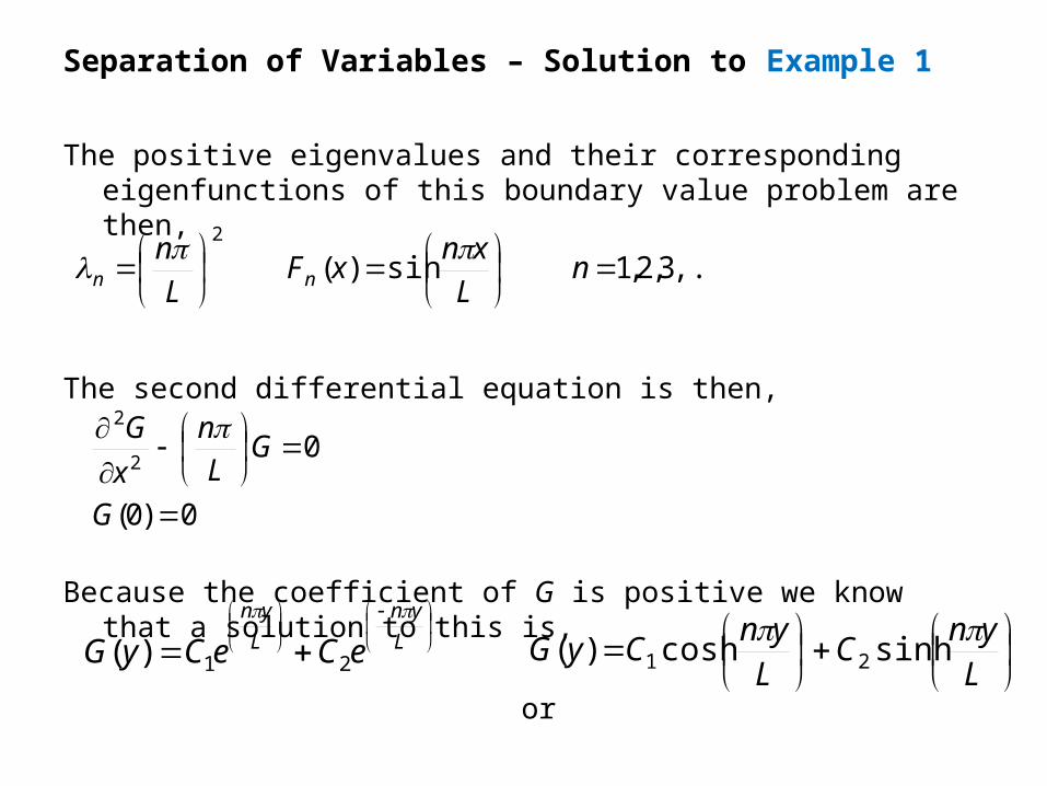
The positive eigenvalues and their corresponding eigenfunctions of this boundary value problem are then,

The second differential equation is then,

Because the coefficient of G is positive we know that a solution to this is,

or


,...3,2,1 sin)( 2

n

L

xnxF

L

nnn

0)0(

02

2

G

GL

n

x

G

L

ynC

L

ynCyG

sinhcosh)( 21

L

yn

L

yn

eCeCyG

21)(

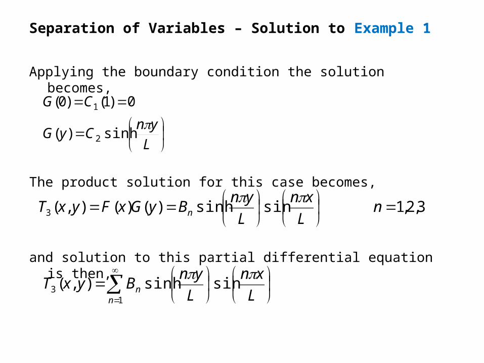
Applying the boundary condition the solution becomes,

The product solution for this case becomes,

and solution to this partial differential equation is then,


L

ynCyG

CG

sinh)(

0)1()0(

2

1

3,2,1 sinsinh)()(),(3

n

L

xn

L

ynByGxFyxT n

13 sinsinh),(

nn L

xn

L

ynByxT

Finally, let’s apply the nonhomogeneous boundary condition to get the coefficients for this solution.

As expected, this is again a Fourier sine series and so using previously done work instead of using the orthogonally of the sines to we see that,


123 sinsinh)(),(

nn L

xn

L

HnBxfHxT

,...3,2,1 sin)(sinh

2

,...3,2,1 sin)(2

sinh

0

2

0

2

ndxL

xnxf

L

HnL

B

ndxL

xnxf

LL

HnB

L

n

L

n

Finally we see that the solution for this problem is:

Where

• Important remarks: For the Laplace equation, the sign of the separation constant and the sequencing of the boundary conditions needs to be decided on a case-by-case basis. However the following rule of thumb can be used as guidance: “Anticipating the edge along which the eventual Fourier series will take place, chose the or - so as to obtain oscillatory functions along that edge. Then apply the boundary conditions adjacent to that edge first”.


13 sinsinh),(

nn L

xn

L

ynByxT

,...3,2,1 sin)(sinh

2

0

2

ndxL

xnxf

L

HnL

BL

n

Consider f(x), to be a constant, say f(x)=100C and our rectangular body to have dimensions L=200, H=100. In this case, we can see the boundary conditions taking place in the eastern, western, and southern boundary were T=0.

Separation of Variables – Visualization of Example 1

http://dylanh.bol.ucla.edu/CA/temperature.html

http://dylanh.bol.ucla.edu/CA/temperature.html

Find a solution to the following PDE

Boundary conditions:

Notice that this example is a part of our original problem solution, it would be the fourth component of our solution.

Separation of Variables – Example 2

024

2

24

2

42

y

T

x

TT

0),(

0)0,(

0),(

)(),0(

4

4

4

14

HxT

xT

yLT

ygyT

T4(L,y)=g2(y)

T1(x,0)=f1(x)

T3(0,y)=g1(y)

T2(x,H)=f2(x)

T1(L,y)=0

T1(x,0)=f1(x)

T1(0,y)=0

T1(x,H)=0

T2(L,y)=g2(y)

T2(x,0)=0

T2(0,y)=0

T2(x,H)=0

T3(L,y)=0

=g2(y)T3(x,0)=f1(x)

T3(0,y)=0

T3(x,H)= f2(x)

= + +T4(L,y)=0

T4(x,0)=0

T4(0,y)= g1(y)

T4(x,H)=0

+

T4(L,y)=0

T4(x,0)=0

T4(0,y)= g1(y)

T4(x,H)=0

We start from assuming the solution can be solved by separating the variable.

Boundary conditions:

Next, we plug the product solution into the differential equation.


)()(),(4 yGxFyxT

0)( 0)0( 0)( HGGLF

2

2

2

2

2

2

2

2

2

2

2

2

11

0)()(

0)()()()(

y

GGx

FF

y

GxF

x

FyG

yGxFy

yGxFx

At this point we need to choose a separation constant, in this case (), Note how the selection of this variable depends on where we have two boundary conditions.

So, after adding in the separation constant we get,

and two ordinary differential equations that we get from this case (along with their boundary conditions) are

and


2

2

2

2 11

y

GGx

FF

0)(

02

2

LF

Fx

F

0)(

0)0(

02

2

LG

G

Gy

G

This time our second ODE has the sine, cosine, solution:

Applying our boundary conditions we get to determine that

The positive eigenvalues and their corresponding eigenfunctions of this boundary value problem are then,


)sin()cos()( 21 yCyCyG

0)0( 1 CG

,...3,2,1 sin)( 2

n

H

ynyG

H

nnn

The second differential equation is then,

Because the coefficient of F is positive we know that a solution to this is,

However, this is not really suited for dealing with the h(L)= 0 boundary condition. So, let’s also notice that the following is also a solution:

This is usually called a “shifted solution” and is very useful!


0)(

02

2

LF

FL

n

x

F

H

xnC

H

xnCxF

sinhcosh)( 21

H

LxnC

H

LxnCxF

)(sinh

)(cosh)( 21

Applying the lone boundary condition to this “shifted” solution gives,

The solution to the first differential equation is now,

And this is all the farther we can go with this because we only had a single boundary condition. That is not really a problem however because we now have enough information to form the product solution for this partial differential equation. A product solution for this partial differential equation is,


0)1()( 1 CLF

H

LxnCxF

)(sinh)( 2

3,2,1 sin)(

sinh)()(),(

n

Hxn

HLxn

ByGxFyxT nn

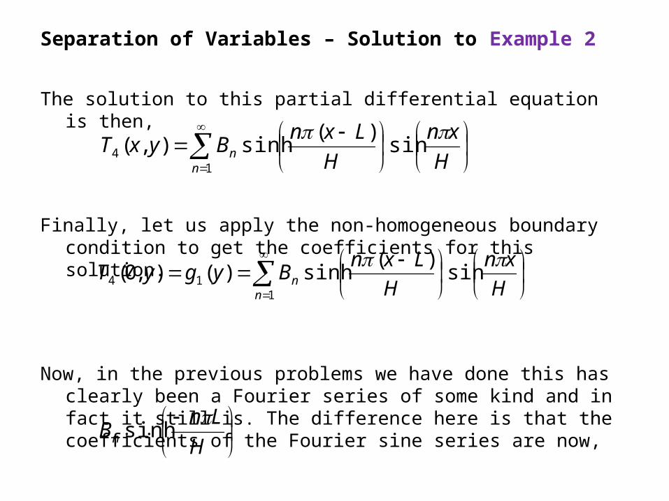
The solution to this partial differential equation is then,

Finally, let us apply the non-homogeneous boundary condition to get the coefficients for this solution.

Now, in the previous problems we have done this has clearly been a Fourier series of some kind and in fact it still is. The difference here is that the coefficients of the Fourier sine series are now,


1

4 sin)(

sinh),(n

n H

xn

H

LxnByxT

1

14 sin)(

sinh)(),0(n

n H

xn

H

LxnBygyT

H

LnBn

sinh

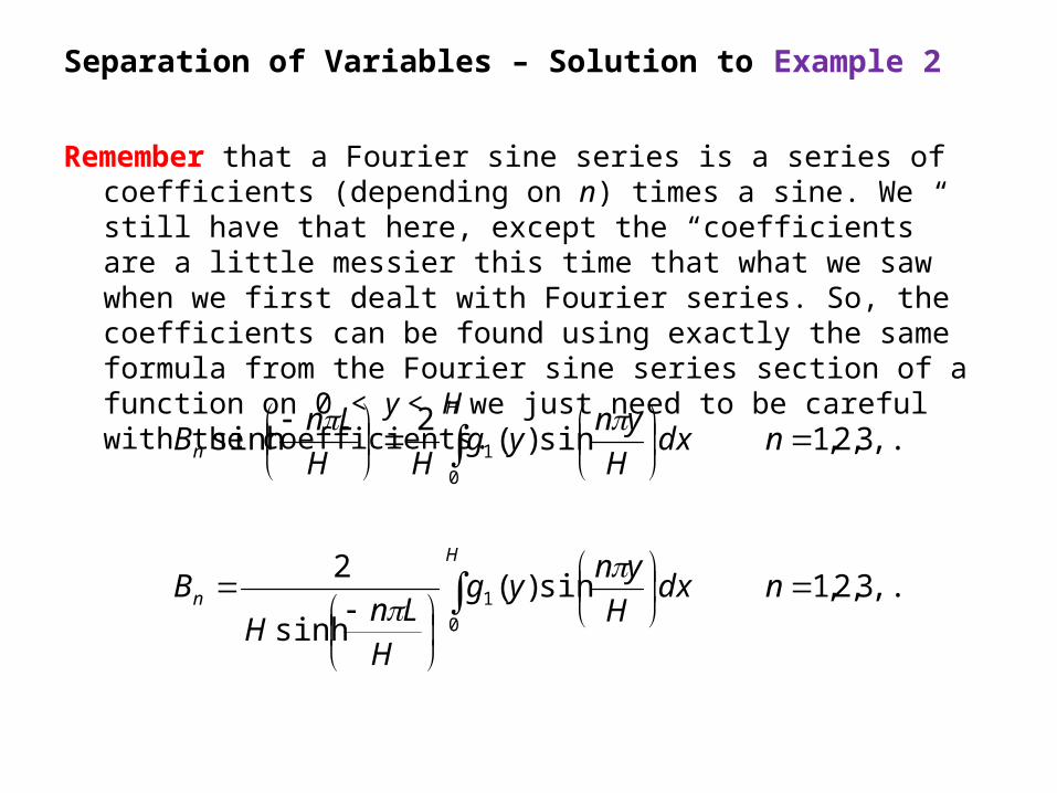
Remember that a Fourier sine series is a series of coefficients (depending on n) times a sine. We still have that here, except the “coefficients” are a little messier this time that what we saw when we first dealt with Fourier series. So, the coefficients can be found using exactly the same formula from the Fourier sine series section of a function on 0 < y < H we just need to be careful with the coefficients.


,...3,2,1 sin)(

sinh

2

,...3,2,1 sin)(2

sinh

0

1

0

1

ndxH

ynyg

H

LnH

B

ndxH

ynyg

HH

LnB

H

n

H

n

Finally we see that the solution for this problem is:

Where


1

4 sin)(

sinh),(n

n H

xn

H

LxnByxT

,...3,2,1 sin)(sinh

2

0

1

ndxH

ynyg

H

LnH

BH

n

Until this point we have worked two of the four cases (T3 &T4)

that would need to be solved in order to completely solve the Laplace equation with non-homogenous boundary conditions in all four sides.

As we have seen each case was similar and yet also had some differences. We saw the use of both separation constants and that sometimes we need to use a “shifted” solution in order to deal with one of the boundary conditions. The remaining cases can be easy to find after this explanation.

Separation of Variables – Closing of Examples 1&2

T4(L,y)=g2(y)

T1(x,0)=f1(x)

T3(0,y)=g1(y)

T2(x,H)=f2(x)

T1(L,y)=0

T1(x,0)=f1(x)

T1(0,y)=0

T1(x,H)=0

T2(L,y)=g2(y)

T2(x,0)=0

T2(0,y)=0

T2(x,H)=0

T3(L,y)=0

=g2(y)T3(x,0)=f1(x)

T3(0,y)=0

T3(x,H)= f2(x)

= + +T4(L,y)=0

T4(x,0)=0

T4(0,y)= g1(y)

T4(x,H)=0

+

The figure on the right illustrates the solution of the Laplace equation with non-homogeneous boundary conditions for al four sides, in this case fixed temperature in all four sides a square body such as the one in the problem.

http://tigger.uic.edu/~rkodama/

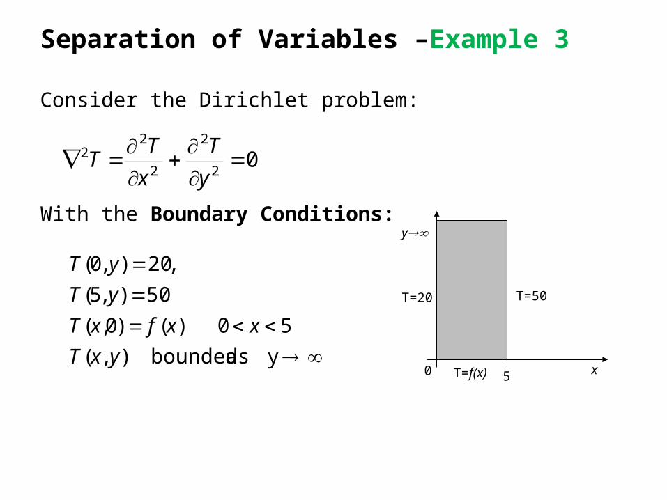
Consider the Dirichlet problem:

With the Boundary Conditions:

Separation of Variables –Example 3

02

2

2

22

y

T

x

TT

T=50

T=f(x)

T=20

0 x

y

5

y as bounded ),(

50 )()0,(

50),5(

,20),0(

yxT

xxfxT

yT

yT

This example can very well represent a complicated three dimensional domain. Take for example the following figure from Greenberg’s book:

Suppose that our interest is finding the temperature of the object near the end of the fin, within the rectangle ABCE, assume we don’t know the boundary along AB and the boundaries T=20 along AE, T=50 along BC, and T=f(x) along EC. To a good approximation, we render the problem tractable by letting D be the entire semi-infinite strips shown for the Dirichlet problem.

Separation of Variables –Example 3

Fig. Cooling fin*

*Greenberg, M. D. (1998). Advanced Engineering Mathematics (2nd ed.): Prentice Hall.

We assume the solution can be solved by separating the variable. In other words the solution is in the form:

We apply this to the homogeneous boundary conditions first since we’ll need those once we get reach the point of choosing the separation constant. The boundary conditions become,

Next, we plug the product solution into the differential equation.

Separation of Variables –Solution of Example 3

)()(),( yGxFyxT

)()0( 50)5( 20)0( xfGFF

2

2

2

2

2

2

2

2

2

2

2

2

11

0)()(

0)()()()(

y

GGx

FF

y

GxF

x

FyG

yGxFy

yGxFx

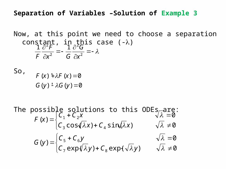
Now, at this point we need to choose a separation constant, in this case (-)

So,

The possible solutions to this ODEs are:


2

2

2

2 11

x

G

Gx

F

F

0)(')'(

0)(')'(

yGyG

xFxF

0 )exp()exp(

0 )(

0 )sin()cos(

0 )(

87

65

43

21

yCyC

yCCyG

xCxC

xCCxF

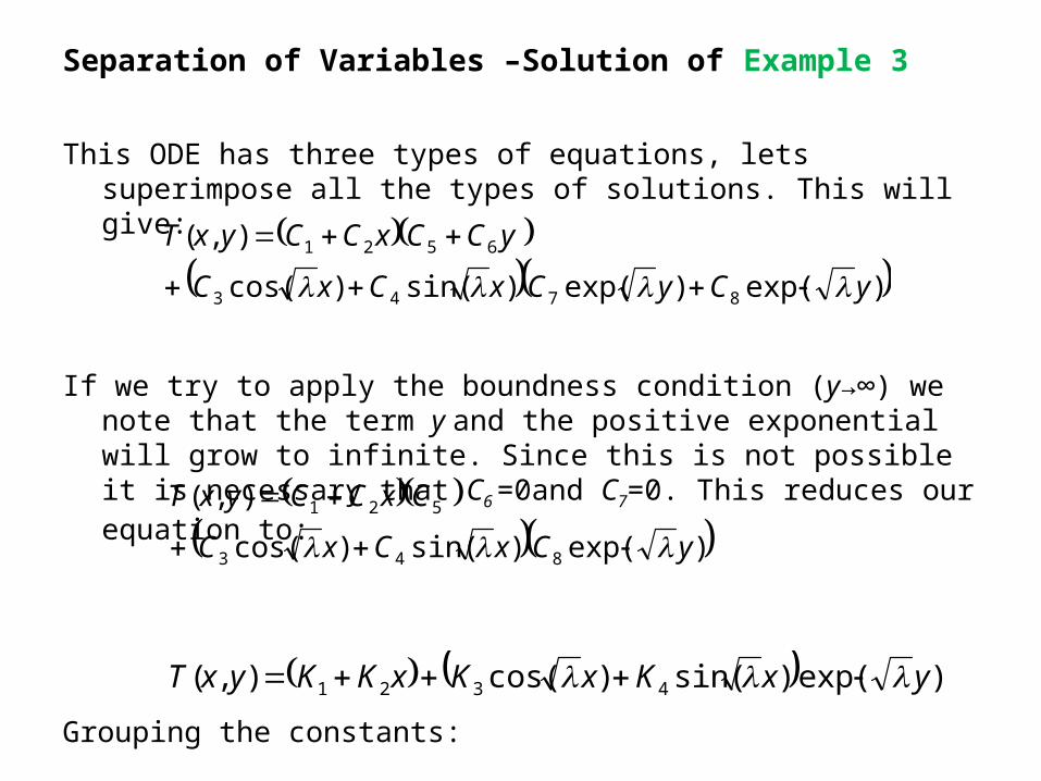
This ODE has three types of equations, lets superimpose all the types of solutions. This will give:

If we try to apply the boundness condition (y→∞) we note that the term y and the positive exponential will grow to infinite. Since this is not possible it is necessary that C6 =0and C7=0. This reduces our equation to:

Grouping the constants:


)exp()exp()sin()cos(

),(

8743

6521

yCyCxCxC

yCCxCCyxT

)exp()sin()cos(

),(

843

521

yCxCxC

CxCCyxT

)exp()sin()cos(),( 4321 yxKxKxKKyxT

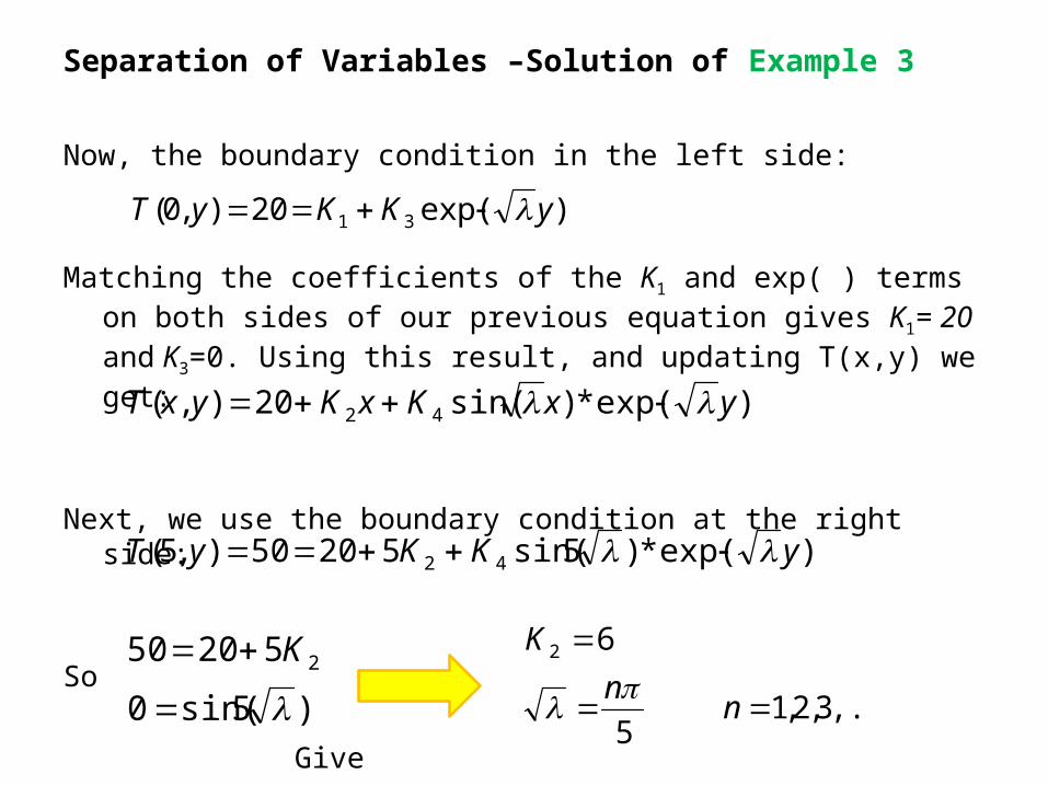
Now, the boundary condition in the left side:

Matching the coefficients of the K1 and exp( ) terms on both sides of our previous equation gives K1= 20 and K3=0. Using this result, and updating T(x,y) we get:

Next, we use the boundary condition at the right side:

So

Give


)exp(20),0( 31 yKKyT

)exp(*)sin(20),( 42 yxKxKyxT

)exp(*)5sin(52050),5( 42 yKKyT

)5sin(0

52050 2

K

,...3,2,1 5

62

nn

K

Using this result to update T(x,y):

This is the solution to our problem. Now we only need to find the value of Kn. To do this we use the lower boundary condition:

We find that

or


1 5exp*

5sin620),(

nn

ynxnKxyxT

1 5sin620)()0,(

nn

xnKxxfxT

1 5sin620)(

nn

xnKxxf

xxfxn

Kn

n 620)(5

sin1

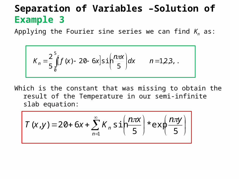
Applying the Fourier sine series we can find Kn as:

Which is the constant that was missing to obtain the result of the Temperature in our semi-infinite slab equation:


,...3,2,1 5

sin620)(5

25

0

ndx

xnxxfKn

1 5exp*

5sin620),(

nn

ynxnKxyxT

20.3 Separation of variables; Non-Cartesian Coodinates

The laplacian in terms of polar coordinates where r, θ are independent variables

which is same as equation (24) from section 16.7

20.3.1 Plane polar coordinates

θ

x

y

r cosθ

r sinθ

r

r

1

rr

1

r 2

2

22

22

From figure polar coordinates can be written in terms of Cartesian coordinates

sinry

cosrx

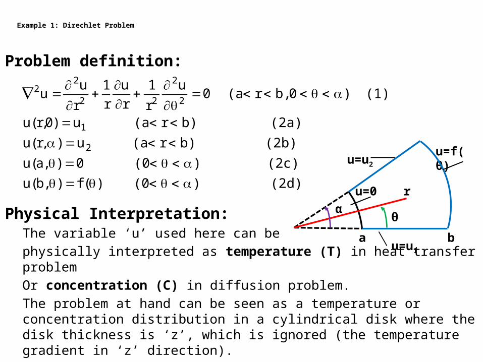
Example 1: Direchlet Problem

Problem definition:

Physical Interpretation:The variable ‘u’ used here can be physically interpreted as temperature (T) in heat transfer problemOr concentration (C) in diffusion problem. The problem at hand can be seen as a temperature or concentration distribution in a cylindrical disk where the disk thickness is ‘z’, which is ignored (the temperature gradient in ‘z’ direction).

(2d) )(0 )(f),b(u

(2c) )(0 0),a(u

(2b) b)r(a u),r(u

(2a) b)r(a u)0,r(u

(1) )0 b,r(a 0u

r

1

r

u

r

1

r

uu

2

1

2

2

22

22

u=0

u=f(θ)

θ

r

a b

u=u2

u=u1

α

Solution using separation of variables method

We seek solution in the form of

Using this as solution the laplacian equation transforms into:

Which can be simplified r and divide by RΘ to separate the variables

Here +κ2 is chosen to obtain solution in the form of cosκθ and sinκθ instead of coshκθ and sinhκθ since we anticipate that to satisfy the u(b,θ)=f(θ) boundary condition we need to expand f(θ) in a Fourier series (discussed later sections)

(3) )()r(R),r(u

(4) 0Rr

1R

r

1R

2

(5) constantR

RrRr 22

The previous differential equation can be written in a more familiar form as

The solution can be written as:

and

Superposition of these two solutions (8a, 8b), we can write a general solution as

(7) 0 and

(6) 0RRrRr2

22

(8a) 0 DrCr

0 rlnBA)r(R

(8b) 0 sin H cosG

0 FE)(

(9) )sin H cosG)(DrCr()FE)(rlnBA(),r(u

Note:A, B, C,D E,F, G, H are arbitrary integration constants and needs to be evaluated.

Apply boundary conditionsWhen θ=0

Set AE=u1 , B=0, and G=0 which gives

When θ=α

So u1+Iα=u2 and sinkα=0 gives

(9) )sin H cosG)(DrCr()FE)(rlnBA(),r(u

u=0

u=f(θ)

θ

r

a b

u=u2

u=u1

α

)(0 )(f),b(u

)(0 0),a(u

b)r(a u),r(u

b)r(a u)0,r(u

2

1

(10) G)DrCr(E)rlnBA(u)0,r(u 1

Boundary conditions

(11) sin )Qr(PrIu),r(u 1

(12) sin )Qr(PrIuu),r(u 11

(13a) 1,2,3...)(n n and

(13a) )uu(I 12

We can write the solution after substituting equation 13a, 13b

Using next boundary condition:

Which can be written as:

Where

(14) n

sinrQrP)uu(u),r(u1n

/nn

/nn121

(2c) )(0 0),a(u

(15) n

sinaQaP)uu(u0),a(u1n

/nn

/nn121

(16) n

sinaQaP)uu(u1n

/nn

/nn121

(17) dn

sin)uu(u2

aQaP0

121/n

n/n

n

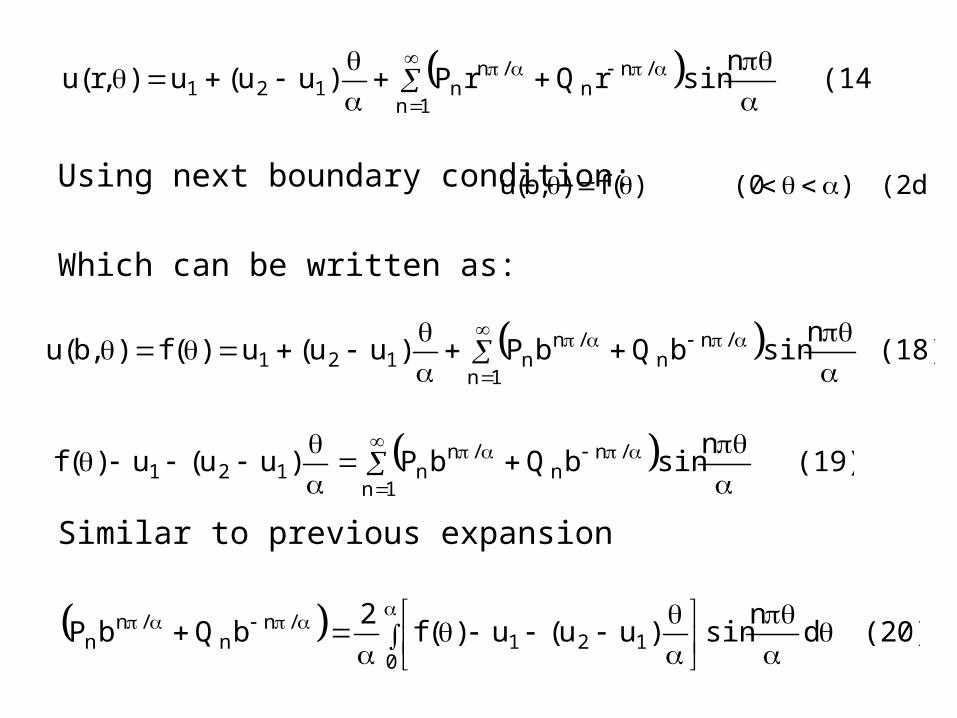
Using next boundary condition:

Which can be written as:

Similar to previous expansion

(14) n

sinrQrP)uu(u),r(u1n

/nn

/nn121

(2d) )(0 )(f),b(u

(18) n

sinbQbP)uu(u)(f),b(u1n

/nn

/nn121

(19) n

sinbQbP)uu(u)(f1n

/nn

/nn121

(20) dn

sin)uu(u)(f2

bQbP0

121/n

n/n

n

Integrals in Equations (17) and (19) can be evaluated when f(θ) is specified which allows us to render them into algebraic equations. They can be solved to obtain a unique solution because the determinant matrix of coefficients is not zero.

0b

a

b

a

bb

aa/n/n

/n/n

/n/n

Numerical Example: Temperature distribution

)(0 100),b(T

)(0 0),a(T

b)r(a 0),r(T

b)r(a 0)0,r(T

)0 b,r(a 0T

r

1

r

T

r

1

r

TT

2

2

22

22

Solution: Using the general solution from previous derivation

n

sinrQrP)TT(T),r(T1n

/nn

/nn121

Apply boundary conditions in above equation

n

sinrQrP),r(T1n

/nn

/nn

Evaluate Pn and Qn by solving the algebraic equations below:

0 dn

sin02

aQaP0

/nn

/nn

n

400 1-

ncos

200 d

nsin100

2bQbP

0

/nn

/nn

and

Solving above algebraic equations we get

0aQaP /nn

/nn

n

400bQbP /n

n/n

n

Final solution for temperature distribution in disk is given by following equation

nsin

ba

ab

ra

ar

n

1400),r(T

1n/n/n

/n/n

/n/n

/n

n

ba

ba

aQ

/n/n

/n

n

ba

ba

aP

20.3.2 Cylindrical coordinates

rθ

z

b

Z=0 Z=L

zz

sinry

cosrx

(1) zr

1

rr

1

r 2

2

2

2

22

22

The laplacian in terms of polar coordinates where r, θ,z are independent variables

(2) 0zr

1

rr

1

r 2

2

2

2

22

22

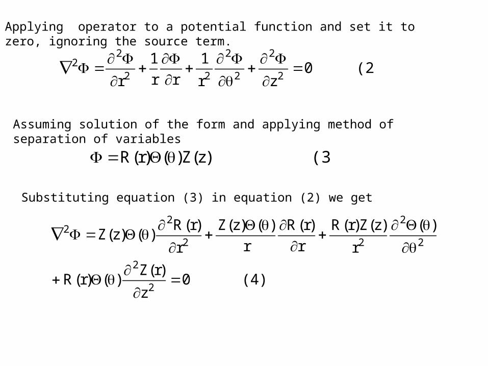
Applying operator to a potential function and set it to zero, ignoring the source term.

(3) )z(Z)()r(R

Assuming solution of the form and applying method of separation of variables

(4) 0z

)r(Z)()r(R

)(

r

)z(Z)r(R

r

)r(R

r

)()z(Z

r

)r(R)()z(Z

2

2

2

2

22

22

Substituting equation (3) in equation (2) we get

(5) 0z

Z

Z

1

r

1

r

R

Rr

1

r

R

R

12

2

2

2

22

2

Simplify by dividing by ) )z(Z)()r(R

Or separating ‘Z’ term

(6) z

Z

Z

1

r

1

r

R

Rr

1

r

R

R

12

2

2

2

22

2

Equations for the three components of solution can be written as follows

For “Z” component

(7.1) 0Zkz

Z

kz

Z

Z

1

22

2

22

2

and use short hand notation for brevity

(7.2) 0v22

2

For “θ”

component

For “R” component

(7.3) 0Rr

vk

r

R

r

1

r

R2

22

2

2

Equation (7.3) is also known as Bessele Equation

Solutions for equations (7.1), (7.2) is well known

(8) e)z(Z kz

(9) e)( ivand

Solution to equation (7.3) is little more complicated, we will it find case by case below

(10) )kr(JR v The solution is in terms of bessel function… Jv(kr)

The solution to the equation that is regular at origin is

Case 1: kr<<1 (11) )kr()kr(J vv

Case 1: kr>>1

References

(12) 42

vkrcos

kr

2)kr(Jv

(1) http://planetmath.org/encyclopedia/LaplaceEquationInCylindricalCoordinates.html

(2) http://www.owlnet.rice.edu/~hill/phys532/L1b.pdf (3) Arfken, George, Weber, Hans, Mathematical Physics. Academic

Press, San Diego, 2001

http://planetmath.org/encyclopedia/LaplaceEquationInCylindricalCoordinates.html

http://planetmath.org/encyclopedia/LaplaceEquationInCylindricalCoordinates.html

http://www.owlnet.rice.edu/~hill/phys532/L1b.pdf

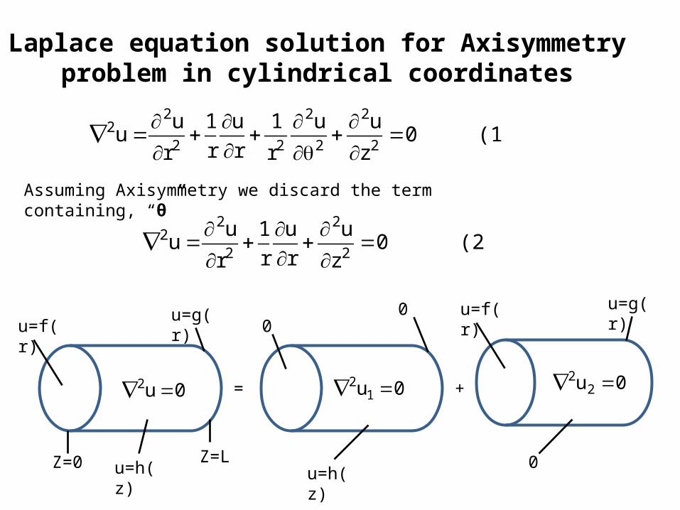
Laplace equation solution for Axisymmetry problem in cylindrical coordinates

(1) 0z

uu

r

1

r

u

r

1

r

uu

2

2

2

2

22

22

Assuming Axisymmetry we discard the term containing, “θ”

(2) 0z

u

r

u

r

1

r

uu

2

2

2

22

0u2 = +0u12 0u2

2

u=f(r)

u=g(r) 0

u=h(z)

0 u=f(r)

0

u=g(r)

u=h(z)

Z=0

Z=L

By superposition of solution as shown in figure we find solution in two parts one for u1 and u2

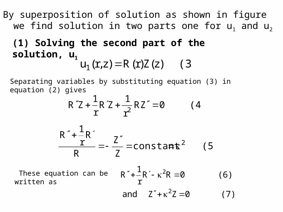
(3) )z(Z)r(R)z,r(u1 Separating variables by substituting equation (3) in equation (2) gives

(5) constantZ

Z

R

Rr

1R

2

(4) 0ZRr

1ZR

r

1ZR

2

These equation can be written as

(7) 0ZZ and

(6) 0RRr

1R

2

2

(1) Solving the second part of the solution, u1

(8) 0k )kr(DK)kr(CI

0k rlnBAR

00

(9) 0k kzsinHkzcosG

0k FzEZ

Solutions for the previous differentiation equations

I0 and K0 are modified bessel functions of the first and second kind, respectively of zero order

The general solution is

(10) )zsin Hz cosG))(kr(DK)kr(CI(

)FZE)(rlnBA()z,r(u

00

Greenberg, M. D. (1998). Advanced Engineering Mathematics (2nd ed.): Prentice Hall.

Applying boundary conditions and simplifying the final solution is

L)z(0 L

znsin)

L

bn(IT)z(h)z,b(u

1n0n1

dz L

znsin)z(h

L

2

L

bnIT

L

00n

Or

dz L

znsin)z(h

L

bnLI

2T

L

00

n


(1) )z(Z)r(R)z,r(u2

(2) Solving the second part of the solution, u2

Separating variables by substituting equation and then writing the solution as done previously…

(2) 0k )kr(DY)kr(CJ

0k rlnBAR

00

(3) 0k kzsinhHkzcoshG

0k FzEZ

J0 and Y0 are modified bessel functions of the first and second kind, respectively of zero order

(4) )zsinh Hz coshG))(kr(DY)kr(CJ(

)FZE)(rlnBA()z,r(u

00

Applying boundary conditions and simplifying the final solution is

(5) b

rzsinhT

b

rzcoshS)

b

rz(J)z,r(u nnnn

1nn02

(6) rdrb

rzJ)r(f

)]z(J[b

2S

b

0n02

n12n

(7) rdrb

rzJ)r(g

)]z(J[b

2)

b

rzsinh(T)

b

rzcosh(S

b

0n02

n12nnnn

Final solution is obtained by solving equation (6) and equation (7) and substituting equation (5)

The complete solution to the problem on ‘u’ is as below

)z,r(u)z,r(u)z,r(u 21

20.3.3 Spherical coordinates

(1) 0sin

1sin

sin

112

2

22

22

Laplace equation in spherical coordinates can be written as follows:

(2) )(Q)(P)r(Rz,,r

(3) 0Q

sinQ

1Psin

sinP

1R

R

12

2

2222

2

Substituting equation (2) and simplifying

(4) 0Q

Q

1Psin

P

sinR

R

sin2

22

2

Multiply with r2 sin2 (φ)

(5) 0QmQ 22

2

For “θ” component

This has a solution that is already known

(6) ..0,1,2,3...m e)(Q im

http://users.aber.ac.uk/ruw/teach/260/laplace.php


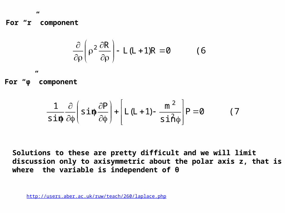
For “r” component

(6) 0R)1L(LR2

For “φ” component

(7) 0Psin

m)1L(L

Psin

sin

12

2

Solutions to these are pretty difficult and we will limit discussion only to axisymmetric about the polar axis z, that is where the variable is independent of θ



Assuming Axisymmetry for Polar axis

Boundary condition

(2) )()(Rz,,r

(1) )(0 )(f),c(

This is analogous problem to the Direchlet problem in polar coordinates

The solution is in the form of

(3) kconstant cot

R

R2R 22

The ODE’s from equation (3)

(4) 0RkR2R 22

(5) 0kcot 2

(6) cosx Change of variables


Change of variables to x gives us

(7) 0)1L(Ldx

dx2

dx

d)x1(

2

22

Note that if x=-1, +1 are excluded from the problem “L” may be a non-integer.The solution to equation (7) is the Legendre polynomial discussed in chapter 4, section 4.3 We will thus write the general solution to Laplace’s equation in spherical coordinates for this case as follows:

(8) cosPr

1BrA),r( L

0n1LL

LL

The Legendre polynomials can be obtained from the following equation (for details refer to section 4.3 in textbook)

(9) 1xdx

d

!L2

1)x(P

L2L

L

LL Rodrigues’ formula

The Legendre polynomials can also obtained from generating function given below:

(10) )x(P)x21(

1),x(F

0LL

L2/12

Note: The polynomials form a complete, orthogonal set of function in the domain of -1<=x<=1 or 0<=θ<=π

(11.2) dx)x(P)x(f2

1L2A

1

1LL

(11.1) )x(PA)x(f0L

LL

Which gives us below equation (11.2) using Fourier Legendre expansion of the function in equation (11.1)


Now using the given boundary conditions in equation (2) for dirichlet problem

(8) cosPr

1BrA),r( L

0n1LL

LL

In this equation we have BL =0 because of stipulated boundaries given. Therefore from equation (8) we have the following final equation

(11) cosP rA),r(0n

LL

L

Use next boundary condition to solve for the constant AL

(12) cosPrA)(f),r(0n

LL

L

Dirichlet Problem in Spherical Coordinates:

We already obtained equations for constants in general solution in previous slides

(12) cosPcA)(f),r(0n

LL

L

From equation 11.2 we can write AL as follows

(14) dsin)(cosP)(fc2

1L2A

1

1LLL

(13) dx)x(P)x(f2

1L2cA

1

1L

LL

Equation (14) and Equation (14) form the final solution for the dirichlet problem for spherical coordinates

20.4 The Fourier Transform

Transform:In mathematics, a function that results when a given function is multiplied by a so-called kernel function, and the product is integrated between suitable limits. (Britannica)

We can use a Fourier transform on x if the x domain isOr a Fourier cosine or sine transform on x if the domain is

x

x0

Application condition

0

st .dt)t(fesLf)s(F

1. http://ase.tufts.edu/chemistry/sykes2.Greenberg, M. D. (1998). Advanced Engineering Mathematics (2nd ed.): Prentice Hall.

http://ase.tufts.edu/chemistry/sykes

http://ase.tufts.edu/chemistry/sykes

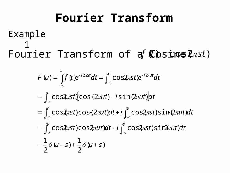
Fourier Transform of a Cosine

Fourier Transform

)2cos()( sttf

Example1

)(2

1)(

2

1

)2sin()2cos()2cos()2cos(

)2sin()2cos()2cos()2cos(

)2sin()2cos()2cos(

)2cos()()( 22

susu

dtutstidtutst

dtutstidtutst

dtutiutst

dtestdtetfuF utiuti

Fourier TransformExample1:Dirichlet problem for Half

Plane

)(for )()0,(

)0 ,(for 0),(2

xxfxu

yxyxu

y

x

Solution by Fourier Transform

1.Apply the Fourier transform in x to the Laplace’s equation (note: y is independent of x )

2. Use Operational Formula

3.Find the general solution of the resulting equation

www.faculty.kfupm.edu.sa/MATH/ffairag/math470_091/notes/6p9b.ppt

Fourier Transform

yy

xi

xi

yyxx

yyxx

BeAeyu

udy

udor

dxeyxu

dy

du

dxey

uui

uFuF

FuuF

),(ˆ

0ˆˆ

0),(

0ˆ)(

0

0

22

2

2

22

2

22

We assume that

0),(lim

),(lim),(ˆlim

0),(

dxeyxu

dxeyxuyu

get

asyyxu

xi

y

xi

yy

We need A=0,so

Solution

y

y

y

y

efyu

Bfu

fu

Beyu

)(ˆ),(ˆ

)(ˆˆ

)(ˆˆ

),(ˆ

0

0


Fourier Transform

Solution

We obtain the final result

dfyxPd

yx

fyyxu )(),(

)(

)(),(

22

This is the Poisson integral formula for the half plane

Poisson kernel


Figure: Poisson kernel P

Helpful References

• Greenberg, M. D. (1998). Advanced Engineering Mathematics (2nd ed.): Prentice Hall.

• Kreyszig, E. (1998). Advanced Engineering Mathematics (8th ed.): Wiley.

• http://tutorial.math.lamar.edu/Classes/DE/LaplacesEqn.aspx

• http://users.aber.ac.uk/ruw/teach/260/laplace.php

http://tutorial.math.lamar.edu/Classes/DE/LaplacesEqn.aspx

http://tutorial.math.lamar.edu/Classes/DE/LaplacesEqn.aspx



End of chapter 20

CHAPTER 20 LAPLACE EQUATION Team 6: Bhanu Kuncharam Tony Rochav Wei Lu.

Documents

Transcript of CHAPTER 20 LAPLACE EQUATION Team 6: Bhanu Kuncharam Tony Rochav Wei Lu.