Chapter 2 — What is Aggregate?Draft version: September 13, 2021

Contents

1 Di�erence Attacks 2

2 Reconstruction Attacks 22.1 Example: Reconstruction Attacks and the Census . . . . . . . . . . . . . . . . . . 3

2.2 The Reconstruction Paradigm . . . . . . . . . . . . . . . . . . . . . . . . . . . . . 4

2.3 Reconstruction from Noisy Statistics . . . . . . . . . . . . . . . . . . . . . . . . . 4

3 Provable Reconstruction Attacks: Linear Reconstruction 53.1 Linear Queries and Linear Reconstruction Attacks . . . . . . . . . . . . . . . . . . 5

3.2 Privacy is an Exhaustible Resource: Reconstruction from Many Queries . . . . . . 7

3.3 Reconstruction Using Fewer Queries . . . . . . . . . . . . . . . . . . . . . . . . . 9

3.3.1 ∗∗ Proving Theorem 3.6 . . . . . . . . . . . . . . . . . . . . . . . . . . . . 10

3.3.2 ∗∗ Do the queries have to be random? . . . . . . . . . . . . . . . . . . . . 11

3.4 Computationally E�cient Reconstruction: Linear Programming . . . . . . . . . . 12

3.5 Can we Improve The Attacks? . . . . . . . . . . . . . . . . . . . . . . . . . . . . . 13

4 Summary 15

1

Acknowledgement. This book chapter is an extension from the course material jointly devel-

oped by Jonathan Ullman and Adam Smith. Please feel free to provide feedback.

We’ve talked about the fact that a lot of the public discussion around data privacy centers

on concepts like identi�ability, speci�cally whether or not an attacker can identify information

belonging to a speci�c individual. So we might come into this subject with the intuition that

aggregate statistics—those which combine the information of many individuals—are automatically

private because there is no direct way to identify any individual in the output. The goal of this

chapter is to disabuse the reader of this notion, and argue that releasing seemingly harmless statistics

can reveal a lot about individuals. We’ll begin with simple examples of di�erence attacks showing

that even questions that seem to aggregate information, when constructed carefully, can actually

single out individuals precisely. However, the bulk of this chapter is devoted to reconstruction

attacks, which allow an attacker to recover all or part of a dataset using noisy statistics. Not only

will we see that reconstruction attacks are possible, we will see that they are, in fact, inevitable if

we don’t impose limits on the kind and amount of information we release about the dataset.

1 Di�erence Attacks

Let’s start with a very simple example. You’ve just started a new job and signed up for the health

insurance provided by your employer. Your employer has access to aggregate statistics from the

insurance provider, and can, in particular ask questions like Howmany employees joined the company

on December 10th, 2020 and have lupus? Suppose the answer to this query is 1. Since the employer

knows your exact start date, and perhaps even knows that you are the only person with this start

date, your employer just learned that you su�er from lupus.

Maybe this example was a little too obvious. If the answer is 1, are we really aggregating

anything? What if we just suppress these small answers and return something like “less than 5”

instead of the exact answer? It turns out that small answers are not the only issue. We can come up

with two queries whose answers are both large, but whose di�erence reveals information about a

speci�c person. Consider the following pair of queries: (1) How many employees joined the company

before December 10th, 2020 and su�er from lupus? (2) How many employees joined the company before

December 11th, 2020 and su�er from lupus? Suppose the answers to these queries are 417 and 418,

respectively. Then, your employer has just learned that you su�er from lupus. Notice that we don’t

need to allow a user to construct carefully related queries for this type of attack to occur. These

are exactly the queries that would arise from a system that reports a running count of the number

of employees with lupus over time, and these sorts of frequently updated statistics often directly

result in di�erence attacks.

Attacks like these that exploit the di�erence between two aggregate queries to single out a

speci�c person are called, unsurprisingly, di�erence attacks.

Di�erence attacks might seem trivial and easily avoided, but they are a useful test case

for any proposed method for protecting privacy.

2 Reconstruction Attacks

We will turn our attention to a much more general class of attacks called reconstruction attacks,

where seemingly benign information can be used to recover a large amount of information about

2

the dataset.

2.1 Example: Reconstruction Attacks and the Census

We’ll introduce reconstruction attacks by way of an example inspired by the U.S. Census Bureau’s

disclosure control methods for the 2010 Decennial Census [GAM19]. The Census collects the age,

sex, race, location, and other demographic information of those living in the United States.

Microdata

ID Block Age Sex Race

001 1402 26 M Black

002 1402 34 F White

003 1402 46 M White

004 1402 30 M Black

005 1402 9 F White

006 1402 5 F White

007 1403 58 F Asian

008 1403 18 F Latina

Tabulations for Block 1402

Age

Statistic Group Count Median Mean

1 Total 6 26 25

2A Female 3 9 16

2B Male 3 30 34

3A Black Male ∗ ∗ ∗

3B Black Female ∗ ∗ ∗

3C White Female 3 9 16

3D White Male ∗ ∗ ∗

Figure 1: An oversimpli�ed example of Census microdata (left) and summary statistics (right).

This data is made available for various purposes, but federal law prohibits releasing the individ-

ual responses—called microdata—so the Census instead releases tabulations of various summary

statistics, such as those in Figure 1.1

As we discussed, releasing small counts is problematic, so

certain cells in the table are suppressed, which we indicate with the ∗ symbol.

What can we learn about the microdata from the tabulations given in Figure 1? Let’s look

at a concrete example and focus on just Statistic 2B in the table, which tells us about the set of

individuals in the dataset who reported their sex as male. The �rst column tells us that there are

three such people in the dataset, so let’s denote their ages as A ≤ B ≤ C . We have the background

information that 0 ≤ A,B,C ≤ 122, where the upper bound is the oldest reported age of any

human.2

Using only our background information, there are

(125

3

)= 317,750 possible choices for A,

B, and C . However, we also know that the median age of these individuals is B = 30, which leaves

us with 31 × 93 = 2,883 possible choices—more than 100-fold fewer choices! Finally, we know that

the mean age of these individuals is1

3(A+ B +C) = 34. Since we know B = 30 and A+ B +C = 108,

we also have C = 78 − A, so C is actually determined once we pick a value of A. That leaves us

with only 31 possible tuples (A,B,C) that are consistent with the given statistics—over 10,000-fold

fewer choices than we started with, from just two statistics! It’s not hard to see how adding more

constaints will quickly reveal even more information about the underlying microdata.

Exercise 2.1. Suppose we unsuppress Statistic 3A, and it shows that the dataset contains two

Black males, whose mean age is 28. Is this enough information to uniquely determine the values A,

B, and C , or are there multiple choices of A,B,C that are consistent with the tabulated statistics?

1Note that the example statistics in Figure 1 are intentionally oversimpli�ed for pedagogical purposes. In particular,

the census asks two separate questions for race and ethnicity and the set of possible responses is much richerd.

2Although it’s the subject of some controvery, the French woman Jeanne Calment reportedly lived to 122 [Wik21].

3

2.2 The Reconstruction Paradigm

The previous reconstruction attack relied on ad hoc reasoning to perform the reconstruction.

However, the approach we took is actually very general, and we can introduce a model to study this

paradigm. We start with some dataset x that represents the underlying microdata. Each statistic (or

query) on the dataset is some function f (x), and for each statistic we obtain some answer f (x) = a.

For example, the �rst column of Statistic 2B tells us that f (x) = 3 where f counts the number of

individuals who entered male as their sex. Each statistic gives us a set of constraints on the dataset,

such as the fact that x must be a dataset with three males.

Tables like the one in Figure 1 give us a large set of constraints like

f1(x) = a1 f2(x) = a2 · · · fk (x) = ak

Given all these constraints, the dataset reconstruction problem is to �nd a dataset x that is consistent

with these constraints.

Aggregate statistics place constraints on the dataset that can be used to reconstruct all or

part of the underlying microdata.

If we are given enough constraints, then there may only be a single consistent dataset, in which

case we have reconstructed the microdata! More generally, the statistics might severely limit what

datasets are consistent, revealing a lot of information about the microdata. In our previous example

we were not able to reconstruct the entire dataset x exactly, but we were able to determine that any

consistent dataset must have three males, one of whom was exactly 30, one younger than 30, and

one of whom was no older than 78.

In general, solving dataset reconstruction is an instance of what are called constraint-satisfaction

problems. Although most interesting constraint-satisfaction problems are NP-hard in the worst

case, we can often use powerful tools like SAT-solvers to do dataset reconstruction in practice,

so NP-hardness o�ers little-to-no practical defense against reconstruction. Moreover, in the next

section we’ll see examples where the reconstruction problem can be solved in polynomial time.

2.3 Reconstruction from Noisy Statistics

Our example of the Census relied only on exact statistics, such as the fact that there were exactly

three males in the dataset. Reconstructing using exact statistics is already enough to cause concern,

and to suggest that some explicit steps must be taken to limit access to sensitive data, such attacks

can be rather brittle and easily avoided. In realistic settings we are not only given a limited set of

statistics to work with, but are also given statistical information that is noisy. For example, the

tabulations in Figure 1 already anticipate certain simple attacks by suppressing certain cells with

small counts, which can be thought of as a form of noise if we think of each suppressed cell as

representing some default answer. Noisy statistics can also arise by explicitly perturbing the data

or the statistics with random noise. Noisy statistical information can be viewed as giving us soft

constraints on the dataset of the form

f1(x) ≈ a1 f2(x) ≈ a2 · · · fk (x) ≈ ak

and reconstruction attacks aim to �nd a dataset x that is consistent with these soft constraints.

4

3 Provable Reconstruction Attacks: Linear Reconstruction

In this section we’ll explore settings where we can rigorously analyze reconstruction attacks, which

will lead to insights about what types of statistical information will leave the microdata vulnerable

to reconstruction, how robust these reconstruction attacks are to sources of noise in the statistics,

and how to carry out these attacks in a computationally e�cient way. This theory was introduced in

a seminal paper by Dinur and Nissim [DN03] that was ultimately the beginning of the development

of di�erential privacy, however we will see the theory presented in a slightly di�erent way that

emphasizes how these attacks might arise in practice.

3.1 Linear Queries and Linear Reconstruction Attacks

Let’s start by introducing a model for reconstruction attacks that will allow us to study the problem

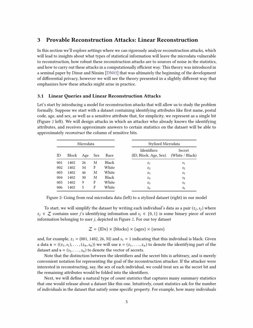
formally. Suppose we start with a dataset containing identifying attributes like �rst name, postal

code, age, and sex, as well as a sensitive attribute that, for simplicity, we represent as a single bit

(Figure 2 left). We will design attacks in which an attacker who already knows the identifying

attributes, and receives approximate answers to certain statistics on the dataset will be able to

approximately reconstruct the column of sensitive bits.

Microdata

ID Block Age Sex Race

001 1402 26 M Black

002 1402 34 F White

003 1402 46 M White

004 1402 30 M Black

005 1402 9 F White

006 1402 5 F White

Stylized Microdata

Identi�ers Secret

(ID, Block, Age, Sex) (White / Black)

z1 s1z2 s2z3 s3z4 s4z5 s5z6 s6

Figure 2: Going from real microdata data (left) to a stylized dataset (right) in our model

To start, we will simplify the dataset by writing each individual’s data as a pair (zj , sj ) where

zj ∈ Z contains user j’s identifying infomation and sj ∈ {0, 1} is some binary piece of secret

information belonging to user j, depicted in Figure 2. For our toy dataset

Z = {IDs} × {blocks} × {ages} × {sexes}

and, for example, z1 = (001, 1402, 26, M) and s1 = 1 indicating that this individual is black. Given

a data x = ((z1, s1), . . . , (zn , sn)) we will use z = (z1, . . . , zn) to denote the identifying part of the

dataset and s = (s1, . . . , sn) to denote the vector of secrets.

Note that the distinction between the identi�ers and the secret bits is arbitrary, and is merely

convenient notation for representing the goal of the reconstruction attacker. If the attacker were

interested in reconstructing, say, the sex of each individual, we could treat sex as the secret bit and

the remaining attributes would be folded into the identi�ers.

Next, we will de�ne a natural type of count statistics that captures many summary statistics

that one would release about a dataset like this one. Intuitively, count statistics ask for the number

of individuals in the dataset that satisfy some speci�c property. For example, how many individuals

5

are older than 28 and have the secret bit 1? Since we’re interested in reconstructing the secret bits

sj , we will only consider statistics of the form

f (x) =n∑j=1

φ(zj )sj for φ : Z → {0, 1}

= #{j : φ(zj ) = 1 and sj = 1} (1)

Here, φ in the example above would be φ(zj ) = 1 if and only if user j is older than 28. Note that if

the microdata contains n individuals, then these statistics return an integer between 0 and n.

The nice thing about these statistics—and the reason they are often called linear statistics—is

because the can be expressed nicely in the language of linear algebra. For a given statistic f and

dataset x with identi�ers z and secret vector s, the value of the statistic has the form

f (x) = fz · s where fz = (φ(z1), . . . ,φ(zn)) (2)

where u · v is the dot product between the two vectors. We used the notation fz to indicate that

the vector depends on both the speci�cation of the query and on the identifying information in

the dataset, however, from now on we will simply write f without the superscript because the

identi�ers will be �xed and unchanging throughout our analysis.

Given a set of queries f1, . . . , fk we can write the evaluation of all the queries as a matrix-vector

product F · s f1(x)...

fk (x)

=

— f1 —

...

— fk —

s1...

sn

(3)

An important thing to note is that, in this notation, the answer to fi is the dot product of the i-throw of the matrix, denoted Fi , with the secret vector s . In other words

fi (x) = (F · s)i = fi · s (4)

Internalizing this notation will help with what comes next. Linear algebra is tricky, and it might

seem daunting to go from something relatively intuitive like a count statistic to matrices and

vectors. However, this linear algebraic representation is going to be crucial both for analyzing how

reconstruction is possible and for making the algorithm computationally e�cient.

Exercise 3.1. Consider the set of queries f1, f2, f3 speci�ed by:

• φ1(zj ) = 1 if and only if user j is older than 40

• φ2(zj ) = 1 if and only if user j is older than 40 and male

• φ3(zj ) = 1 if and only if user j is older than 20 and male

For the dataset in Figure 2, write the matrix F, the secret vector s , and the product F · s.

The reconstruction problem we’re going to try to understand is how to take a vector of approx-

imate answers a ≈ F · s and recover a vector s ≈ s. We’ll mostly focus on when the constraints give

enough information to reconstruct something close to s, and only touch upon how to actually �nd

s in a computationally e�cient way.

6

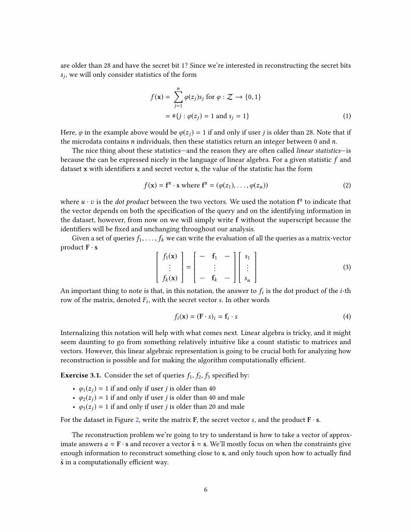
In this chapter, we will only see one actual reconstruction attack, although we’ll prove di�erent

things about it depending on which queries we’re given. All the attack does is try to �nd a vector

of secrets s ∈ {0, 1}n that is consistent with the information we’re given, in the sense that we would

have obtained similar answers if the true secrets were s. See Algorithm 1 for a description of the

attack.

Algorithm 1 The Reconstruction Attack

1: Reconstruct(f1, . . . , fk ;a1, . . . ,ak ; z)2: input: queries f1, . . . , fk , answers a1, . . . ,ak ∈ R, and identi�ers z ∈ Zn

3: output: a vector of secrets s ∈ {0, 1}n

4: form the vectors f1, . . . , fk using the queries and identi�ers

5: let s ∈ {0, 1}n be the vector that minimizes the quantity maxi ∈[k ] |fi · s − ai |6: return s

To be explicit, we’ve de�ned the reconstruction attack in terms of the queries f1, . . . , fk and the

identi�ers, but ultimately what the attack needs is only the vector representation f1, . . . , fk , so as a

shorthand we will sometimes say that the attack is “given” the vector representation of the queries.

The next claim captures a simple, but important statement about what happens in this recon-

struction attack when the answers are all accurate to within some error bound.

Claim 3.2. If every query is answered to within error ≤ αn, i.e.

max

i ∈[k ]|fi · s − ai | ≤ αn,

then the reconstruction attack returns s such that maxi ∈[k ] |fi · s − ai | ≤ αn.

To see why this claim is true, observe that the true vector of secrets s satis�esmaxi ∈[k ] |fi ·s−ai | ≤αn. Thus, the vector s that minimizes this quantity must make it no greater than αn. We may

actually �nd a vector s that minimizes the quantity even further, but for our analysis we will only

use the fact that there is some s that has error ≤ αn for these queries.

The main idea for how we’re going to analyze this attack is to show that for every s that

disagrees with the real s in many coordinates, there is some query vector fi that prevents s from

being the minimum in the sense that |fi · s− fi · s| is too large, and therefore |fi · s− ai | is also large.

3.2 Privacy is an Exhaustible Resource: Reconstruction from Many Queries

In case you’re wondering, so far we have not shown that there is any set of statistics that can be

used to reconstruct the secret vector s, even when we are given exact answers to each of these

statistics. But such sets do exist! We leave it as an exercise to write down an explicit example.

Exercise 3.3. Suppose the identi�ers z1, . . . , zn are unique and known to you. Construct a set of

statistics f1, . . . , fn such that, for every secret vector s ∈ {0, 1}n , the reconstruction attack will

recover s = s provided it is given exact answers to each of these queries so that ai = fi (x).

But can reconstruction succeed when the answers are noisy? In this section we’ll prove a

simple, but absolutely crucial result, showing that if we are given answers to all possible statistics,

then reconstruction is possible even if the noise in the queries is so large as to render the answers

almost useless.

7

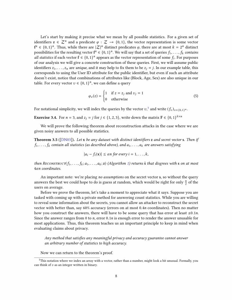
Let’s start by making it precise what we mean by all possible statistics. For a given set of

identi�ers z ∈ Znand a predicate φ : Z → {0, 1}, the vector representation is some vector

fz ∈ {0, 1}n . Thus, while there are |Z|n distinct predicates φ, there are at most k = 2n

distinct

possibilities for the resulting vector fz ∈ {0, 1}n . We will say that a set of queries f1, . . . , fk contains

all statistics if each vector f ∈ {0, 1}n appears as the vector representation of some fi . For purposes

of our analysis we will give a concrete construction of these queries. First, we will assume public

identi�ers z1, . . . , zn are unique, and it may help to �x them to be zj = j. In our example table, this

corresponds to using the User ID attribute for the public identi�er, but even if such an attribute

doesn’t exist, notice that combinations of attributes like (Block, Age, Sex) are also unique in our

table. For every vector v ∈ {0, 1}n , we can de�ne a query

φv (z) =

{1 if z = zj and vj = 1

0 otherwise

(5)

For notational simplicity, we will index the queries by the vector v ,3

and write (fv )v ∈{0,1}n .

Exercise 3.4. For n = 3, and zj = j for j ∈ {1, 2, 3}, write down the matrix F ∈ {0, 1}k×n

We will prove the following theorem about reconstruction attacks in the case where we are

given noisy answers to all possible statistics.

Theorem 3.5 ([DN03]). Let x be any dataset with distinct identi�ers z and secret vector s. Then if

f1, . . . , fk contain all statistics (as described above), and a1, . . . ,ak are answers satisfying

|ai − fi (x)| ≤ αn for every i = 1, . . . ,k,

then Reconstruct(f1, . . . , fk ;a1, . . . ,ak ; z) (Algorithm 1) returns s that disgrees with s on at most

4αn coordinates.

An important note: we’re placing no assumptions on the secret vector s, so without the query

answers the best we could hope to do is guess at random, which would be right for onlyn2

of the

users on average.

Before we prove the theorem, let’s take a moment to appreciate what it says. Suppose you are

tasked with coming up with a private method for answering count statistics. While you are willing

to reveal some information about the secrets, you cannot allow an attacker to reconstruct the secret

vector with better than, say 60% accuracy (errors on at most 0.4n coordinates). Then no matter

how you construct the answers, there will have to be some query that has error at least ±0.1n.

Since the answer ranges from 0 to n, error 0.1n is enough error to render the answer unusable for

most applications. Thus, this theorem teaches us an important principle to keep in mind when

evaluating claims about privacy.

Any method that satis�es any meaningful privacy and accuracy guarantee cannot answer

an arbitrary number of statistics to high accuracy.

Now we can return to the theorem’s proof.

3This notation where we index an array with a vector, rather than a number, might look a bit unusual. Formally, you

can think of v as an integer written in binary.

8

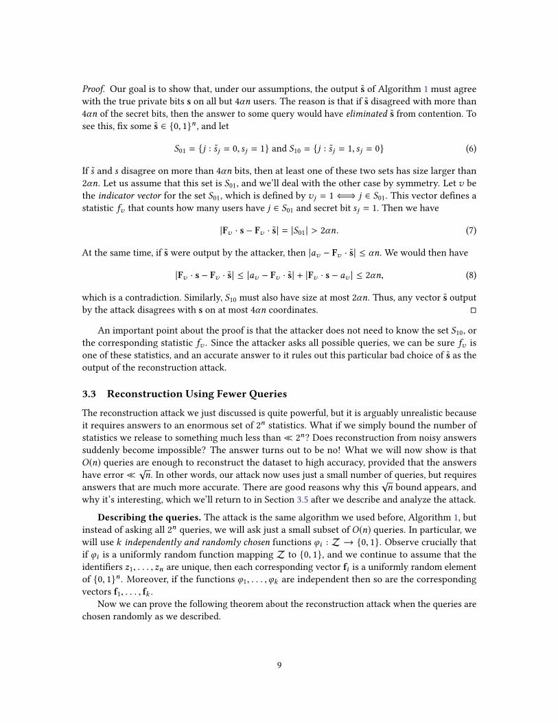
Proof. Our goal is to show that, under our assumptions, the output s of Algorithm 1 must agree

with the true private bits s on all but 4αn users. The reason is that if s disagreed with more than

4αn of the secret bits, then the answer to some query would have eliminated s from contention. To

see this, �x some s ∈ {0, 1}n , and let

S01 = {j : sj = 0, sj = 1} and S10 = {j : sj = 1, sj = 0} (6)

If s and s disagree on more than 4αn bits, then at least one of these two sets has size larger than

2αn. Let us assume that this set is S01, and we’ll deal with the other case by symmetry. Let v be

the indicator vector for the set S01, which is de�ned by vj = 1⇐⇒ j ∈ S01. This vector de�nes a

statistic fv that counts how many users have j ∈ S01 and secret bit sj = 1. Then we have

|Fv · s − Fv · s| = |S01 | > 2αn. (7)

At the same time, if s were output by the attacker, then |av − Fv · s| ≤ αn. We would then have

|Fv · s − Fv · s| ≤ |av − Fv · s| + |Fv · s − av | ≤ 2αn, (8)

which is a contradiction. Similarly, S10 must also have size at most 2αn. Thus, any vector s output

by the attack disagrees with s on at most 4αn coordinates. �

An important point about the proof is that the attacker does not need to know the set S10, or

the corresponding statistic fv . Since the attacker asks all possible queries, we can be sure fv is

one of these statistics, and an accurate answer to it rules out this particular bad choice of s as the

output of the reconstruction attack.

3.3 Reconstruction Using Fewer Queries

The reconstruction attack we just discussed is quite powerful, but it is arguably unrealistic because

it requires answers to an enormous set of 2n

statistics. What if we simply bound the number of

statistics we release to something much less than� 2n

? Does reconstruction from noisy answers

suddenly become impossible? The answer turns out to be no! What we will now show is that

O(n) queries are enough to reconstruct the dataset to high accuracy, provided that the answers

have error�√n. In other words, our attack now uses just a small number of queries, but requires

answers that are much more accurate. There are good reasons why this

√n bound appears, and

why it’s interesting, which we’ll return to in Section 3.5 after we describe and analyze the attack.

Describing the queries. The attack is the same algorithm we used before, Algorithm 1, but

instead of asking all 2n

queries, we will ask just a small subset of O(n) queries. In particular, we

will use k independently and randomly chosen functions φi : Z → {0, 1}. Observe crucially that

if φi is a uniformly random function mapping Z to {0, 1}, and we continue to assume that the

identi�ers z1, . . . , zn are unique, then each corresponding vector fi is a uniformly random element

of {0, 1}n . Moreover, if the functions φ1, . . . ,φk are independent then so are the corresponding

vectors f1, . . . , fk .

Now we can prove the following theorem about the reconstruction attack when the queries are

chosen randomly as we described.

9

Theorem 3.6 ([DN03]). Let x be any dataset with distinct identi�ers z and secret vector s. Then if

f1, . . . , fk are k = 20n independent, uniformly random statistics (as described above) then with high

probability (over the choice of the queries), if a1, . . . ,ak are answers satisfying

|ai − fi (x)| ≤ αn for every i = 1, . . . ,k,

then Reconstruct(f1, . . . , fk ;a1, . . . ,ak ; z) (Algorithm 1) returns s that disagrees with s on at most

256α2n2 coordinates.4

Observe that when α � 1/√n, the reconstruction error is� n, meaning that we recover nearly

all of the secret bits. As we discuss in Section 3.5, introducing error that is proportional to

√n is

signi�cant, because this is the scale of the error that would arise naturally if the data were randomly

sampled from some population. Thus, this theorem teaches us another important lesson.

Any method that o�ers a meaningful privacy guarantee and has “insigni�cant” error is

severely limited in how many queries it can answer.

The proof that this attack has low reconstruction error is much trickier, but ultimately uses the

same idea we used for the exponential reconstruction attack—if s and s disagree on many bits, then

there will be some query that proves s cannot be close to s, and thus cannot be the output of the

reconstruction attack.

3.3.1 ∗∗ Proving Theorem 3.6

Before giving the proof, we’ll need the following technical fact.

Claim 3.7. Let t ∈ {−1, 0,+1}n be a vector with at leastm non-zero entries and let u ∈ {0, 1}n be a

uniformly random vector. Then

P(|u · t| >

√m/4

)≤

1

10

(9)

Proof sketch. Intuitively, what we want to show is that u · t behaves somewhat like a Gaussian

random variable with standard deviation at least

√m/2. If it were truly Gaussian with this standard

deviation, then the probability that it is contained in an any interval of width

√m/2 would be at

most7

10. The reason the right-hand side above is

9

10is because the Gaussian approximation isn’t

exactly correct, and we need to account for the di�erence, which can be done in several ways. We

do not include a complete proof. �

Now let’s return to the proof of Theorem 3.6

Proof of Theorem 3.6. Our goal will be to show that any vector s ∈ {0, 1}n that disagrees with s on

more than 256α2n2 bits cannot satisfy

∀i ∈ [k] |fi · s − ai | ≤ αn. (10)

and thus cannot be the output of the reconstruction attack. To this end, �x any true secret vector

s ∈ {0, 1}n and let

B ={s : s and s disagree on at least 256α2n2 coordinates

}(11)

4The constants 20 and 256 in this theorem are somewhat arbitrary and can de�nitely be improved substantially with

a more careful analysis.

10

Our goal is to show that the reconstruction attack does not output any vector in B. Here B is

a mnemonic for the set of “bad” outputs that we want to show are not the ones returned by the

reconstruction attack. To this end, we will say that statistic i eliminates vector s if

|fi · (s − s)| ≥ 4αn. (12)

If s is eliminated by some statistic i then s cannot be the output of the reconstruction attack because

|fi · s − ai | ≥ |fi · (s − s) − ai | − |fi · s − ai | ≥ 4αn − αn = 3αn. (13)

Thus, our goal is to show that every vector in B is eliminated by some query. In other words

∀s ∈ B ∃i ∈ [k] |Fi · (s − s)| ≥ 4αn (14)

To do so, let’s �x some particular vector s ∈ B and show that it is eliminated with extremely

high probability. Speci�cally, suppose s ∈ {0, 1}n di�ers from s on at leastm = 256α2n2 coordinates.

We will argue

∃i ∈ [k] |fi · (s − s)| ≥ 4αn (15)

We will show how (15) can be deduced from Claim 3.7. Fix vectors s and s that di�er on at least

m coordinates, and de�ne t = s − s. Then t ∈ {−1, 0,+1}n and t has at least m non-zero entries.

Moreover, since the queries are chosen uniformly at random, u = fi is a uniformly random vector

in {0, 1}n . Thus u and t satisfy the assumptions of Claim 3.7, so we conclude that

P (|fi · (s − s)| ≤ 4αn) ≤9

10

(16)

Thus, each query fi has a reasonable chance of eliminating s. Now, since the k = 20n queries are

independent, we have that

P (∀i ∈ [k] : |fi · (s − s)| ≤ 4αn) ≤

(9

10

)20n

≤ 2−2n . (17)

The last step is to argue that every s ∈ B will be eliminated by some statistic i . Since there are

only 2n

possible choices for s, we know that |B| ≤ 2n

Therefore, we have

P (∃s ∈ B , ∀i ∈ [k] : |fi · (s − s)| ≤ 4αn) ≤ 2n · 2−2n = 2

−n . (18)

We now know that (except with probability ≤ 2−n

), every vector s that disagrees with s on more

than m coordinates will be eliminated from contention, so the attacker must return a vector s that

disagrees on at most m coordinates. Note that the only way reconstruction can fail is if we get

unlucky with the choice of queries, which happens with probability at most 2−n

. �

3.3.2 ∗∗ Do the queries have to be random?

Although we modeled the queries, and thus the matrix F, as uniformly random, it’s important to

note that we really only relied on the fact that for every pair of vectors s, s,

max

i ∈[k ]|Fi · (s − s)| &

√err(s, s), (19)

11

where we de�ne err(s, s) is the number of coordinates on which they disagree. We can perform

noisy reconstruction with error ≈√n for any family of queries that gives rise to a matrix with

this property. Moreover, quantitatively weaker versions of this property lead to reconstruction

attacks as well, albeit with less tolerance to noise. Not every matrix satis�es a property like this

one, and later on we will see examples of special types of queries that are much easier to make

private than random queries. However, any family of random enough queries will satisfy such a

property. More speci�cally, this property, or similar properties, are satis�ed by any matrix with no

small singular values [DY08] or high discrepancy [MN12, NTZ13], and these conditions are known

to hold for some natural families such as marginal statistics and contingency tables [KRSU10], and

various geometric families [MN12].

3.4 Computationally E�cient Reconstruction: Linear Programming

Algorithm 1 is not computationally e�cient, even if the number of queries k is small, since the

attacker might have to enumerate all 2n

vectors s ∈ {0, 1}n to �nd one that minimizes

max

i ∈[k ]|fi · s − ai | (20)

However, we can modify the attack slightly to run in time polynomial in n using linear pro-

gramming (see the cutout). To do so, we have to start by �nding some real-valued vector s ∈ [0, 1]n

that solves the following optimization problem

argmin

s ∈[0,1]nmax

i ∈[k ]|fi · s − ai | (21)

Then, to obtain the reconstruction we will round each entry to 0 or 1 to obtain a vector s ∈ {0, 1}n .

Pseudocode for the new attack is in Algorithm 2

Algorithm 2 The LP-Based Reconstruction Attack

1: LP-Reconstruct(f1, . . . , fk ;a1, . . . ,ak ; z)2: input: queries f1, . . . , fk , answers a1, . . . ,ak ∈ R, and identi�ers z ∈ Zn

3: output: a vector of secrets s ∈ {0, 1}n

4: form the vectors f1, . . . , fk using the queries and identi�ers

5: using an LP, �nd s ∈ [0, 1]n that minimizes the quantity maxi ∈[k ] |fi · s − ai |6: let s ∈ {0, 1}n be the vector obtained by rounding each value si to {0, 1}

7: return s

Exercise 3.8. The optimization problem in LP-Reconstruct (Algorithm 2, Line 5) does not look

like LPs as they are de�ned in the cutout but can indeed be written as one. Show how to write an

LP that solves this optimization problem.

Using a very slightly more careful analysis, one can prove that when we are given answers to

O(n) random queries, each with error at most αn, the solution to the linear program will satisfy

n∑j=1

|sj − sj | . α2n2 (22)

12

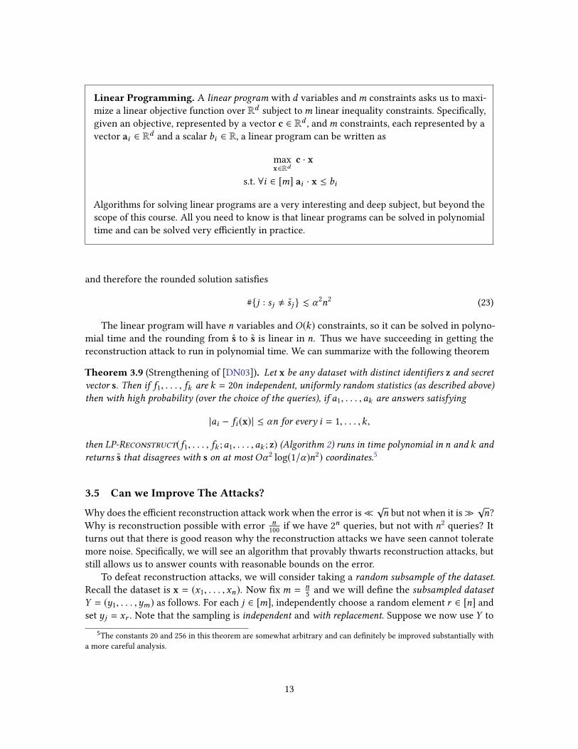
Linear Programming. A linear program with d variables andm constraints asks us to maxi-

mize a linear objective function over Rd subject tom linear inequality constraints. Speci�cally,

given an objective, represented by a vector c ∈ Rd , andm constraints, each represented by a

vector ai ∈ Rd and a scalar bi ∈ R, a linear program can be written as

max

x∈Rdc · x

s.t. ∀i ∈ [m] ai · x ≤ bi

Algorithms for solving linear programs are a very interesting and deep subject, but beyond the

scope of this course. All you need to know is that linear programs can be solved in polynomial

time and can be solved very e�ciently in practice.

and therefore the rounded solution satis�es

#{j : sj , sj } . α2n2 (23)

The linear program will have n variables and O(k) constraints, so it can be solved in polyno-

mial time and the rounding from s to s is linear in n. Thus we have succeeding in getting the

reconstruction attack to run in polynomial time. We can summarize with the following theorem

Theorem 3.9 (Strengthening of [DN03]). Let x be any dataset with distinct identi�ers z and secretvector s. Then if f1, . . . , fk are k = 20n independent, uniformly random statistics (as described above)

then with high probability (over the choice of the queries), if a1, . . . ,ak are answers satisfying

|ai − fi (x)| ≤ αn for every i = 1, . . . ,k,

then LP-Reconstruct(f1, . . . , fk ;a1, . . . ,ak ; z) (Algorithm 2) runs in time polynomial in n and k and

returns s that disagrees with s on at most Oα2log(1/α)n2) coordinates.5

3.5 Can we Improve The Attacks?

Why does the e�cient reconstruction attack work when the error is�√n but not when it is�

√n?

Why is reconstruction possible with errorn100

if we have 2n

queries, but not with n2 queries? It

turns out that there is good reason why the reconstruction attacks we have seen cannot tolerate

more noise. Speci�cally, we will see an algorithm that provably thwarts reconstruction attacks, but

still allows us to answer counts with reasonable bounds on the error.

To defeat reconstruction attacks, we will consider taking a random subsample of the dataset.

Recall the dataset is x = (x1, . . . ,xn). Now �x m = n5

and we will de�ne the subsampled dataset

Y = (y1, . . . ,ym) as follows. For each j ∈ [m], independently choose a random element r ∈ [n] and

set yj = xr . Note that the sampling is independent and with replacement. Suppose we now use Y to

5The constants 20 and 256 in this theorem are somewhat arbitrary and can de�nitely be improved substantially with

a more careful analysis.

13

compute the statistics in place of x. That is, we return the answer

5f (Y ) =m∑j=1

5φ(yj ) (24)

in place of the true answer

f (X ) =n∑j=1

φ(x j ) (25)

Note that we multiply by 5 to account for the fact thatm = n5

.

Releasing the subsampled dataset Y doesn’t seem to provide much, if any, “privacy” to the users.

If a user would be unhappy if you released the full dataset x, then someone who is in the subsample

Y would be just as unhappy or more if you released Y , and since each user in x has a reasonably

large change of being in the subsample, they would probably not be happy with your decision to

release Y before knowing whether or not they land in Y .

However, any reconstruction attack, when given the statistics computed on Y , must have

reconstruction error at least4n10

, because the answers we are revealing do not depend on the users

whose data wasn’t subsampled. Thus the best the attacker can do is learn the secret bit of the users

in the subsample exactly and then guess the secret bit of the other users at random.

However, the random subsample will simultaneously give a good estimate of the answers to

many statistics. Speci�cally, one can prove the following result:

Exercise 3.10. Prove that for any set of statistics f1, . . . , fk , with probability at least99

100,

∀i ∈ [k]����� m∑j=1

5φi (yj ) −n∑i=1

φi (x j )

����� ≤ O(√

n logk)

(26)

Therefore, we see that for k = 20n as in the case of the e�cient reconstruction attack, a

random subsample will prevent reconstruction and give answers with error

√n logn. In contrast,

reconstruction provably succeeds any time the error is�√n, so our reconstruction attack cannot

be improved signi�cantly. Also, when k � 2o(n)

, a random subsample will prevent reconstruction

and answer all queries with error o(n), meaning that no reconstruction attack that makes k = 2o(n)

queries can tolerate noisen100

!

So this is a bit unsatisfying. The reconstruction attacks we have are the best possible, and can

be defeated by a method that doesn’t give a meaningful privacy guarantee. As the course goes

on we will see how to give accurate answers to these statistics with rigorous privacy guarantees

via di�erential privacy [DMNS06]. In some cases, the accuracy will match the limits imposed by

reconstruction attacks and in some cases it won’t. We will also see a more subtle type of privacy

attack called membership inference that can help explain these gaps.

Exercise 3.11. (More general subsampling) Consider a dataset x = (x1, . . . ,xn). For some pa-

rameter m, we will de�ne the subsampled dataset Y = (y1, . . . ,ym) as follows. For each j ∈ [m],independently choose a random element r ∈ [n] and set yj = xr . Note that the sampling is

independent and with replacement. Suppose we now use Y to compute the statistics in place of x.

1. Given Y , how can we obtain an unbiased estimate of a count statistic f (x) =∑n

j=1 φ(x j )?That is, output an estimate f (Y ) such that for every x, E (f (Y )) = f (x).

14

2. What is the variance of your estimate? That is, E((f (Y ) − f (x))2

)?

3. Suppose we are given statistics f1, . . . , fk . Prove the tightest bound you can on the maximum

error of your estimates of fi (Y ) over all i = 1, . . . ,k . That is, prove that, for every dataset x,

P(

kmax

i=1| fi (Y ) − fi (x)| ≤ �

)≥ 1 − β (27)

where you should �ll in � with the best expression you can come up with in terms ofm, k ,

and β .

4 Summary

Key Points

• Aggregate statistics place constraints on the dataset that can be used to reconstruct all or

part of the underlying data about individuals.

• Any method that satis�es any meaningful privacy and accuracy guarantee cannot answer an

arbitrary number of statistics.

• Any method that answers too many queries with an “insigni�cant” amount of error cannot

satisfy any meaningful privacy guarantee.

Additional Reading

• A survey on privacy attacks against aggregate statistics [DSSU17]

• More discussion of reconstruction attacks at

– https://differentialprivacy.org/reconstruction-theory/– https://differentialprivacy.org/diffix-attack/

References

[DMNS06] Cynthia Dwork, Frank McSherry, Kobbi Nissim, and Adam Smith. Calibrating noise to

sensitivity in private data analysis. In Conference on Theory of Cryptography, TCC ’06,

2006.

[DN03] Irit Dinur and Kobbi Nissim. Revealing information while preserving privacy. In

Proceedings of the 22nd ACM Symposium on Principles of Database Systems, PODS ’03.

ACM, 2003.

[DSSU17] Cynthia Dwork, Adam Smith, Thomas Steinke, and Jonathan Ullman. Exposed! A

Survey of Attacks on Private Data. Annual Review of Statistics and Its Application,

4:61–84, 2017.

[DY08] Cynthia Dwork and Sergey Yekhanin. New e�cient attacks on statistical disclosure

control mechanisms. In Annual International Cryptology Conference. Springer, 2008.

15

[GAM19] Simson Gar�nkel, John M Abowd, and Christian Martindale. Understanding database

reconstruction attacks on public data. Communications of the ACM, 62(3):46–53, 2019.

[KRSU10] Shiva Prasad Kasiviswanathan, Mark Rudelson, Adam Smith, and Jonathan Ullman. The

price of privately releasing contingency tables and the spectra of random matrices with

correlated rows. In Proceedings of the 42nd ACM Symposium on Theory of Computing,

STOC ’10. ACM, 2010.

[MN12] S Muthukrishnan and Aleksandar Nikolov. Optimal private halfspace counting via

discrepancy. In Proceedings of the forty-fourth annual ACM symposium on Theory of

computing. ACM, 2012.

[NTZ13] Aleksandar Nikolov, Kunal Talwar, and Li Zhang. The geometry of di�erential privacy:

The small database and approximate cases. In ACM Symposium on Theory of Computing,

STOC ’13, 2013.

[Wik21] Wikipedia contributors. Jeanne calment — Wikipedia, the free encyclope-

dia. https://en.wikipedia.org/w/index.php?title=Jeanne_Calment&oldid=1030629685, 2021. [Online; accessed 28-June-2021].

16