CHAPTER 2 RESCUING THE ECONOMY FROM THE … 2 RESCUING THE ECONOMY FROM THE GREAT ... Rescuing the...
42
39 C H A P T E R 2 RESCUING THE ECONOMY FROM THE GREAT RECESSION T he first and most fundamental task the Administration faced when President Obama took office was to rescue an economy in freefall. In November 2008, employment was declining at a rate of more than half a million jobs per month, and credit markets were stretched almost to the breaking point. As the economy entered 2009, the decline accelerated, with job loss in January reaching almost three-quarters of a million. The President responded by working with Congress to take unprecedented actions. These steps, together with measures taken by the Federal Reserve and other finan- cial regulators, have succeeded in stabilizing the economy and beginning the process of healing a severely shaken economic and financial system. But much work remains. With high unemployment and continued job losses, it is clear that recovery must remain the key focus of 2010. An Economy in Freefall According to the National Bureau of Economic Research, the United States entered a recession in December 2007. Unlike most postwar reces- sions, this downturn was not caused by tight monetary policy aimed at curbing inflation. Although economists will surely analyze this downturn extensively in the years to come, there is widespread consensus that its central precipitating factor was a boom and bust in asset prices, especially house prices. The boom was fueled in part by irresponsible and in some cases predatory lending practices, risky investment strategies, faulty credit ratings, and lax regulation. When the boom ended, the result was wide- spread defaults and crippling blows to key financial institutions, magnifying the decline in house prices and causing enormous spillovers to the remainder of the economy.
Transcript of CHAPTER 2 RESCUING THE ECONOMY FROM THE … 2 RESCUING THE ECONOMY FROM THE GREAT ... Rescuing the...
39
C H A P T E R 2
RESCUING THE ECONOMYFROM THE GREAT RECESSION
The first and most fundamental task the Administration faced whenPresident Obama took office was to rescue an economy in freefall. In
November 2008, employment was declining at a rate of more than half amillion jobs per month, and credit markets were stretched almost to thebreaking point. As the economy entered 2009, the decline accelerated, withjob loss in January reaching almost three-quarters of a million. The Presidentresponded by working with Congress to take unprecedented actions. Thesesteps, together with measures taken by the Federal Reserve and other finan-cial regulators, have succeeded in stabilizing the economy and beginningthe process of healing a severely shaken economic and financial system. Butmuch work remains. With high unemployment and continued job losses, itis clear that recovery must remain the key focus of 2010.
An Economy in Freefall
According to the National Bureau of Economic Research, the UnitedStates entered a recession in December 2007. Unlike most postwar reces-sions, this downturn was not caused by tight monetary policy aimed atcurbing inflation. Although economists will surely analyze this downturnextensively in the years to come, there is widespread consensus that itscentral precipitating factor was a boom and bust in asset prices, especiallyhouse prices. The boom was fueled in part by irresponsible and in somecases predatory lending practices, risky investment strategies, faulty creditratings, and lax regulation. When the boom ended, the result was wide-spread defaults and crippling blows to key financial institutions, magnifyingthe decline in house prices and causing enormous spillovers to the remainderof the economy.
40 | Chapter 2
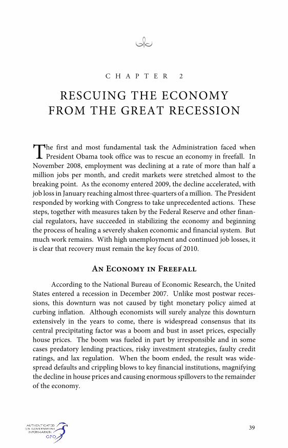
The Run-Up to the RecessionThe rise in house prices during the boom was remarkable. As Figure
2-1 shows, real house prices almost doubled between 1997 and 2006. By2006, they were more than 50 percent above the highest level they hadreached in the 20th century.
Stock prices also rose rapidly. The Standard and Poor’s (S&P) 500,for example, rose 101 percent between its low in 2002 and its high in 2007.That rise, though dramatic, was not unprecedented. Indeed, in the fiveyears before its peak in March 2000, during the “tech bubble,” the S&P 500rose 205 percent, while the more technology-focused NASDAQ index rose506 percent.
The run-up in asset prices was associated with a surge in construc-tion and consumer spending. Residential construction rose sharply asdevelopers responded to the increase in housing demand. From the fourthquarter of 2001 to the fourth quarter of 2005, the residential investmentcomponent of real GDP rose at an average annual rate of nearly 8 percent.Similarly, consumers responded to the increases in the value of their assetsby continuing to spend freely. Saving rates, which had been declining sincethe early 1980s, fell to about 2 percent during the two years before the reces-sion. This spending was facilitated by low interest rates and easy credit, withhousehold borrowing rising faster than incomes.
50
75
100
125
150
175
200
1909 1919 1929 1939 1949 1959 1969 1979 1989 1999 2009
Figure 2-1House Prices Adjusted for Inflation
Index (1900=100)
Sources: Shiller (2005); recent data from http://www.econ.yale.edu/~shiller/data/Fig2-1.xls.
Rescuing the Economy from the Great Recession | 41
The DownturnHouse prices began to drop in some markets in 2006, and then
nationally beginning in 2007. This process was gradual at first, with pricesmeasured using the LoanPerformance house price index declining just3½ percent nationally between January and June 2007. Lenders had lentaggressively during the boom, often providing mortgages whose soundnesshinged on continued house price appreciation. As a result, the compara-tively modest decline in house prices threatened large losses on subprimeresidential mortgages (the riskiest class of mortgages), as well as on theslightly higher-quality “Alt-A” mortgages. As the availability of mortgagecredit tightened, the downward pressure on real estate prices intensified.National house prices declined 6 percent between June and December 2007.
The negative feedback between credit availability and the housingmarket weighed on household and business confidence, restraining consumerspending and business investment. Although residential constructionled the slowdown in real activity through 2007, by early 2008 outlays forconsumer goods and services and business equipment and software haddecelerated sharply, and total employment was beginning to decline. Realgross domestic product (GDP) fell slightly in the first quarter of 2008.
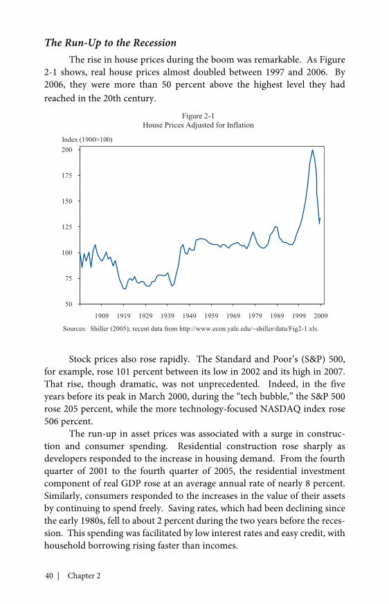
In February 2008, Congress passed a temporary tax cut. Figure 2-2shows real after-tax (or disposable) income and consumer spending beforeand after rebate checks were issued. Consumption was maintained despitea tremendous decline in household wealth over the same period. Totalhousehold and nonprofit net worth declined 9.1 percent between June2007 and June 2008. Microeconomic studies of consumer behavior in thisepisode confirm the role of the tax rebate in maintaining spending (Brodaand Parker 2008; Sahm, Shapiro, and Slemrod 2009). The fact that real GDPreversed course and grew in the second quarter of 2008 is further tributeto the helpfulness of the policy. But, in part because of the lack of robust,sustained stimulus, growth did not continue.
Financial institutions had invested heavily in assets whose values weretied to the value of mortgages. For many reasons—the opacity of the instru-ments, the complexity of financial institutions’ balance sheets and their“off-balance-sheet” exposures, the failure of credit-rating agencies to accu-rately identify the riskiness of the assets, and poor regulatory oversight—theextent of the institutions’ exposure to mortgage default risk was obscured.When mortgage defaults rose, the result was unexpectedly large losses tomany financial institutions.
In the fall of 2008, the nature of the downturn changed dramatically.More rapid declines in asset prices generated further loss of confidencein the ability of some of the world’s largest financial institutions to honor
42 | Chapter 2
their obligations. In September, the Lehman Brothers investment bankdeclared bankruptcy, and other large financial firms (including AmericanInternational Group, Washington Mutual, and Merrill Lynch) were forcedto seek government aid or to merge with stronger institutions. Whatfollowed was a rush to liquidity and a cascading of retrenchment that hadmany of the features of a classic financial panic.
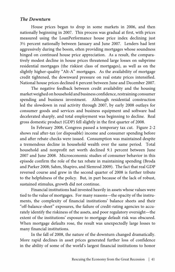
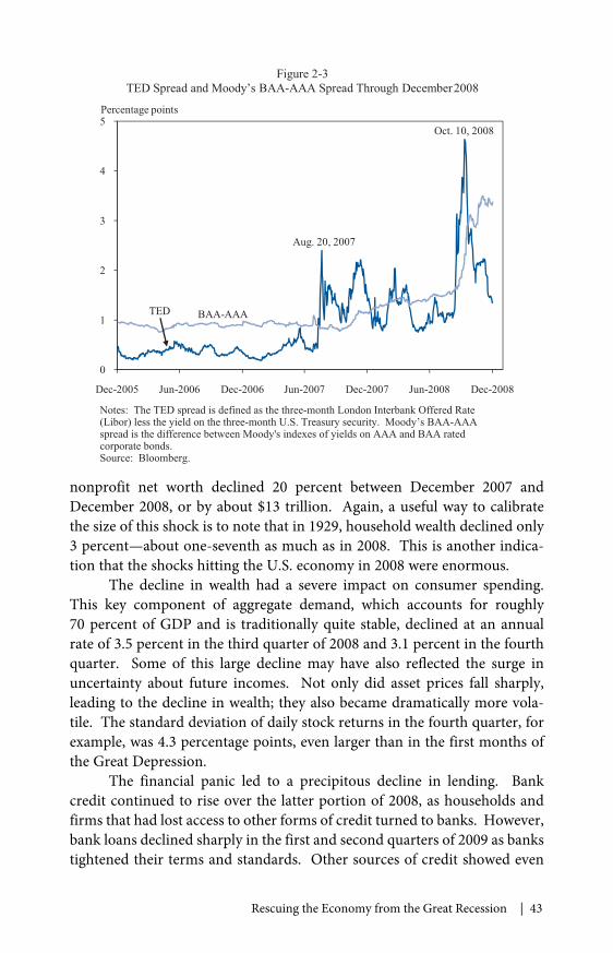
Risk spreads shot up to extraordinary levels. Figure 2-3 shows boththe TED spread and Moody’s BAA-AAA spread. The TED spread is thedifference between the rate on short-term loans among banks and a safeshort-term Treasury interest rate. The BAA-AAA spread is the differencebetween the interest rates on high-grade and medium-grade corporatebonds. Both spreads rose dramatically during the heart of the panic. Indeed,one way to put the spike in the BAA-AAA spread in perspective is to notethat the same spread barely moved during the Great Crash of the stockmarket in 1929, and rose by only about half as much during the first wave ofbanking panics in 1930 as it did in the fall of 2008.
The same loss of confidence shown by the rise in credit spreadstranslated into declining asset prices of all sorts. The S&P 500 declined29 percent in the second half of 2008. Real house prices tumbled another11 percent over the same period (see Figure 2-1). All told, household and
9,000
9,200
9,400
9,600
9,800
10,000
10,200
10,400
Jan-2007 Jul-2007 Jan-2008 Jul-2008 Jan-2009 Jul-2009
Figure 2-2Income and Consumption Around the 2008 Tax Rebate
Billions of 2005 dollars, seasonally adjusted annual rate
Disposable Personal Income
Personal Consumption Expenditures
Sources: Department of Commerce (Bureau of Economic Analysis), National Income andProduct Accounts Table 2.6, line 30, and Table 2.8.6, line 1.
Rescuing the Economy from the Great Recession | 43
nonprofit net worth declined 20 percent between December 2007 andDecember 2008, or by about $13 trillion. Again, a useful way to calibratethe size of this shock is to note that in 1929, household wealth declined only3 percent—about one-seventh as much as in 2008. This is another indica-tion that the shocks hitting the U.S. economy in 2008 were enormous.
The decline in wealth had a severe impact on consumer spending.This key component of aggregate demand, which accounts for roughly70 percent of GDP and is traditionally quite stable, declined at an annualrate of 3.5 percent in the third quarter of 2008 and 3.1 percent in the fourthquarter. Some of this large decline may have also reflected the surge inuncertainty about future incomes. Not only did asset prices fall sharply,leading to the decline in wealth; they also became dramatically more vola-tile. The standard deviation of daily stock returns in the fourth quarter, forexample, was 4.3 percentage points, even larger than in the first months ofthe Great Depression.
The financial panic led to a precipitous decline in lending. Bankcredit continued to rise over the latter portion of 2008, as households andfirms that had lost access to other forms of credit turned to banks. However,bank loans declined sharply in the first and second quarters of 2009 as bankstightened their terms and standards. Other sources of credit showed even
0
1
2
3
4
5
Dec-2005 Jun-2006 Dec-2006 Jun-2007 Dec-2007 Jun-2008 Dec-2008
Figure 2-3TED Spread and Moody’s BAA-AAA Spread Through December2008
Percentage points
Aug. 20, 2007
Oct. 10, 2008
BAA-AAATED
Notes: The TED spread is defined as the three-month London Interbank Offered Rate(Libor) less the yield on the three-month U.S. Treasury security. Moody’s BAA-AAAspread is the difference between Moody's indexes of yields on AAA and BAA ratedcorporate bonds.Source: Bloomberg.
44 | Chapter 2
more substantial declines. One particularly important market is that forcommercial paper (short-term notes issued by firms to finance key operatingcosts such as payroll and inventory). The market for lower-tier nonfinancial(A2/P2) commercial paper collapsed in the fall of 2008, with the averagedaily value of new issues falling from $8.0 billion in the second quarter of2008 to $4.3 billion in the fourth quarter. In addition, securitization ofautomobile loans, credit card receivables, student loans, and commercialmortgages ground to a halt.
This freezing of credit markets, together with the decline in wealthand confidence, caused consumer spending and residential investment tofall sharply. Real GDP declined at an annual rate of 2.7 percent in the thirdquarter of 2008, 5.4 percent in the fourth quarter, and 6.4 percent in thefirst quarter of 2009. Industrial production, which had been falling steadilyover the first eight months of 2008, plummeted in the final four months—dropping at an annual rate of 18 percent.
Many industries were battered by the financial crisis and the resultingeconomic downturn. The American automobile industry was hit particu-larly hard. Sales of light motor vehicles, which had exceeded 16 millionunits every year from 1999 to 2007, fell to an annual rate of only 9.5 millionin the first quarter of 2009. Employment in the motor vehicle and partsindustry declined by 240,000 over the 12 months through January 2009.Two domestic manufacturers, General Motors (GM) and Chrysler, requiredemergency loans in late December 2008 and early January 2009 to avoiddisorderly bankruptcy.
The most disturbing manifestation of the rapid slowdown in theeconomy was the dramatic increase in job loss. Over the first months of2008, job losses were typically between 100,000 and 200,000 per month.In October, the economy lost 380,000 jobs; in November, 597,000 jobs.By January, the economy was losing jobs at a rate of 741,000 per month.Commensurate with this terrible rate of job loss, the unemployment raterose rapidly—from 6.2 percent in September 2008 to 7.7 percent in January2009. It then continued to rise by roughly one-half of a percentage point permonth through the winter and spring; it reached 9.4 percent in May, andended the year at 10.0 percent.
Wall Street and Main StreetAs described in more detail later, policymakers have focused much
of their response to the crisis on stabilizing the financial system. ManyAmericans are troubled by these policies. Because to a large extent it wasthe actions of credit market participants that led to the crisis, people ask whypolicymakers should take actions focused on restoring credit markets.
Rescuing the Economy from the Great Recession | 45
The basic reason for these policies is that the health of credit marketsis critically important to the functioning of our economy. Large firms usecommercial paper to finance their biweekly payrolls and pay suppliers formaterials to keep production lines going. Small firms rely on bank loans tomeet their payrolls and pay for supplies while they wait for payment of theiraccounts receivable. Home purchases depend on mortgages; automobilepurchases depend on car loans; college educations depend on student loans;and purchases of everyday items depend on credit cards.
The events of the past two years provide a dramatic demonstrationof the importance of credit in the modern economy. As the President saidin his inaugural address, “Our workers are no less productive than whenthis crisis began. Our minds are no less inventive, our goods and servicesno less needed.” Yet developments in financial markets—rises and fallsin home and equity prices and in the availability of credit—have led to acollapse of spending, and hence to a precipitous decline in output and tounemployment for millions.
Numerous academic studies before the crisis had also shown that theavailability of credit is critical to investment, hiring, and production. Onestudy, for example, found that when a parent company earns high profitsand so has less need to rely on credit, the additional funds lead to higherinvestment by subsidiaries in completely unrelated lines of business (Lamont1997). Another found that when a small change in a firm’s circumstancesfrees up a large amount of funds that would otherwise have to go to pensioncontributions, the result is a large change in spending on capital goods(Rauh 2006). Other studies have shown that when the Federal Reservetightens monetary policy, small firms, which typically have more difficultyobtaining financing, are hit especially hard (Gertler and Gilchrist 1994), andfirms without access to public debt markets cut their inventories much moresharply than firms that have such access (Kashyap, Lamont, and Stein 1994).
Research before the crisis had also found that financial market disrup-tions could affect the real economy. Ben Bernanke, who is now Chairmanof the Federal Reserve, demonstrated a link between the disruption oflending caused by bank failures and the worsening of the Great Depression(Bernanke 1983). A smaller but more modern example is provided by theimpact of Japan’s financial crisis in the 1990s on the United States: construc-tion lending, new construction, and construction employment were moreadversely affected in U.S. states where subsidiaries of Japanese banks hada larger role, and thus where credit availability was more affected by thecollapse of Japan’s bubble (Peek and Rosengren 2000). That a financialdisruption in a trading partner can have a detectable adverse impact on oureconomy through its impact on credit availability suggests that the effect of
46 | Chapter 2
a full-fledged financial crisis at home would be enormous—an implicationthat, sadly, has proven to be correct.
Finally, microeconomic evidence from the recent crisis also shows theimportance of the financial system to the real economy. For example, firmsthat happened to have long-term debt coming due after the crisis began,and thus faced high costs of refinancing, cut their investment much morethan firms that did not (Almeida et al. 2009). Another study found that amajority of corporate chief financial officers surveyed reported that theirfirms faced financing constraints during the crisis, and that the constrainedfirms on average planned to reduce investment spending, research anddevelopment, and employment sharply compared with the unconstrainedfirms (Campello, Graham, and Harvey 2009).
In short, the goal of the policies to stabilize the financial system wasnot to help financial institutions. The goal was to help ordinary Americans.When the financial system is not working, individuals and businesses cannotget credit, demand and production plummet, and job losses skyrocket.Thus, an essential step in healing the real economy is to heal the financialsystem. The alternative of letting financial institutions suffer the conse-quences of their mistakes would have led to a collapse of credit markets andvastly greater suffering for millions and millions of Americans.
The policies to rescue the financial sector were, however, costly, andoften had the side effect of benefiting the very institutions whose irrespon-sible actions contributed to the crisis. That is one reason that the Presidenthas endorsed a Financial Crisis Responsibility Fee on the largest financialfirms to repay the Federal Government for its extraordinary actions. Asdiscussed in Chapter 6, the Administration has also proposed a compre-hensive plan for financial regulatory reform that will help ensure that WallStreet does not return to the risky practices that were a central cause of therecent crisis.
The Unprecedented Policy Response
Given the magnitude of the shocks that hit the economy in the fall of2008 and the winter of 2009, the downturn could have turned into a secondGreat Depression. That it has not is a tribute to the aggressive and effec-tive policy response. This response involved the Federal Reserve and otherfinancial regulators, the Administration, and Congress. The policy toolswere similarly multifaceted, including monetary policy, financial marketinterventions, fiscal policy, and policies targeted specifically at housing.
Rescuing the Economy from the Great Recession | 47
Monetary PolicyThe first line of defense against a weak economy is the interest rate
policy of the independent Federal Reserve. By increasing or decreasing thequantity of reserves it supplies to the banking system, the Federal Reservecan lower or raise the Federal funds rate, which is the interest rate at whichbanks lend to one another. The funds rate influences other interest ratesin the economy and so has important effects on economic activity. Usingchanges in the target level of the funds rate as their main tool of counter-cyclical policy, monetary policymakers had kept inflation low and the realeconomy remarkably stable for more than two decades.
The Federal Reserve has used interest rate policy aggressively in therecent episode. The target level of the funds rate at the beginning of 2007was 5¼ percent. The Federal Reserve cut the target by 1 percentage pointover the last four months of 2007 and by an additional 2¼ percentage pointsover the first four months of 2008. After the events of September, it cut thetarget in three additional steps in October and December, bringing it to itscurrent level of 0 to ¼ percent.
Conventional interest rate policy, however, could do little to dealwith the enormous disruptions to credit markets. As a result, the FederalReserve has used a range of unconventional tools to address those disrup-tions directly. For example, in March 2008, it created the Primary DealerCredit Facility and the Term Securities Lending Facility to provide liquiditysupport for primary dealers (that is, financial institutions that trade directlywith the Federal Reserve) and the key financial markets in which theyoperate. In October 2008, when the critical market for commercial paperthreatened to stop functioning, the Federal Reserve responded by setting upthe Commercial Paper Funding Facility to backstop the market.
Once the Federal Reserve’s target for the funds rate was effectivelylowered to zero in December 2008, there was another reason to use uncon-ventional tools. Nominal interest rates generally cannot fall below zero:because holding currency guarantees a nominal return of zero, no one iswilling to make loans at a negative nominal interest rate. As a result, whenthe Federal funds rate is zero, supplying more reserves does not drive itlower. Statistical estimates suggest that based on the Federal Reserve’s usualresponse to inflation and unemployment, the subdued level of inflation andthe weak state of the economy would have led the central bank to reduce itstarget for the funds rate by about an additional 5 percentage points if it couldhave (Rudebusch 2009).
This desire to provide further stimulus, coupled with the inability touse conventional interest rate policy, led the Federal Reserve to undertakelarge-scale asset purchases to reduce long-term interest rates. In March
48 | Chapter 2
2009, the Federal Reserve announced plans to purchase up to $300 billion oflong-term Treasury debt; it also announced plans to increase its purchasesof the debt of Fannie Mae, Freddie Mac, and the Federal Home Loan Banks(the government-sponsored enterprises, or GSEs, that support the mortgagemarket) to up to $200 billion, and its purchases of agency (that is, FannieMae, Freddie Mac, and Ginnie Mae) mortgage-backed securities to up to$1.25 trillion.
Finally, the Federal Reserve has attempted to manage expectations byproviding information about its goals and the likely path of policy. Officialshave consistently stressed their commitment to ensuring that inflationneither falls substantially below nor rises substantially above its usual level.In addition, the Federal Reserve has repeatedly stated that economic condi-tions “are likely to warrant exceptionally low levels of the Federal fundsrate for an extended period.” To the extent this statement provides marketparticipants with information they did not already have, it is likely to keeplonger-term interest rates lower than they otherwise would be.
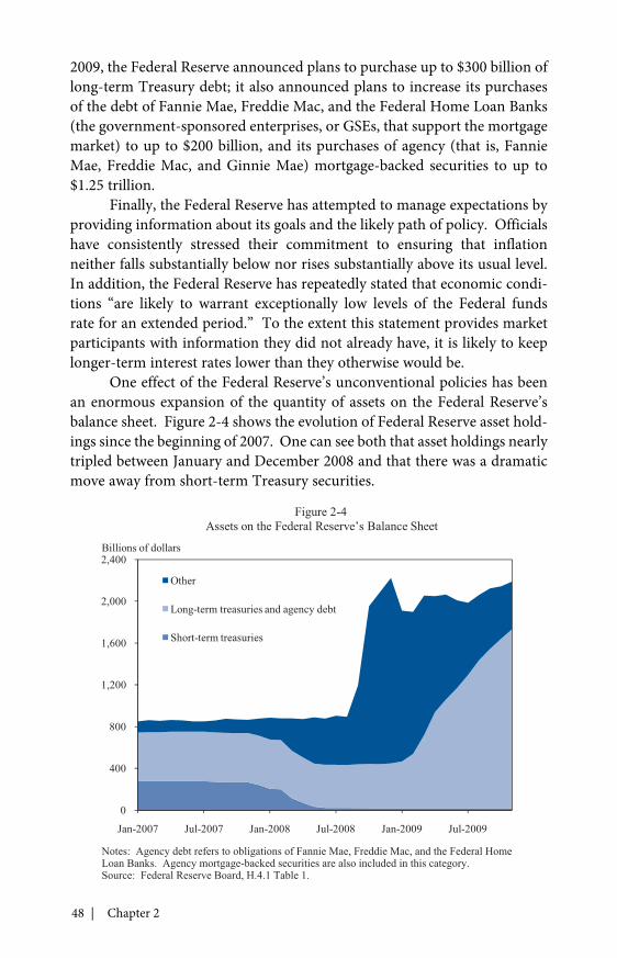
One effect of the Federal Reserve’s unconventional policies has beenan enormous expansion of the quantity of assets on the Federal Reserve’sbalance sheet. Figure 2-4 shows the evolution of Federal Reserve asset hold-ings since the beginning of 2007. One can see both that asset holdings nearlytripled between January and December 2008 and that there was a dramaticmove away from short-term Treasury securities.
0
400
800
1,200
1,600
2,000
2,400
Jan-2007 Jul-2007 Jan-2008 Jul-2008 Jan-2009 Jul-2009
Other
Long-term treasuries and agency debt
Short-term treasuries
Figure 2-4Assets on the Federal Reserve’s Balance Sheet
Billions of dollars
Notes: Agency debt refers to obligations of Fannie Mae, Freddie Mac, and the Federal HomeLoan Banks. Agency mortgage-backed securities are also included in this category.Source: Federal Reserve Board, H.4.1 Table 1.
Rescuing the Economy from the Great Recession | 49
The flip side of the large increase in the Federal Reserve’s assetholdings is a large increase in the quantity of reserves it has supplied to thefinancial system. Some observers have expressed concern that the largeexpansion in reserves could lead to inflation. In this regard, two key pointsshould be kept in mind. First, as already described, most statistical modelssuggest that the Federal Reserve’s target interest rate would be substan-tially lower than it is today if it were not constrained by the fact that theFederal funds rate cannot fall below zero. As a result, monetary policy isin fact unusually tight given the state of the economy, not unusually loose.Second, the Federal Reserve has the tools it needs to prevent the reservesfrom leading to inflation. It can drain the reserves from the financial systemthrough sales of the assets it has acquired or other actions. Indeed, despitethe weak state of the economy, the return of credit market conditions towardnormal is leading to the natural unwinding of some of the exceptional creditmarket programs. Another reliable way the Federal Reserve can keep thereserves from creating inflationary pressure is by using its relatively newability to raise the interest rate it pays on reserves: banks will be unwillingto lend the reserves at low interest rates if they can obtain a higher return ontheir balances held at the Federal Reserve.
Financial RescueEfforts to stabilize the financial system have been a central part of
the policy response. As just discussed, even before the financial crisis inSeptember 2008, the Federal Reserve was taking steps to ease pressureson credit markets. The events of the fall led to even stronger actions. OnSeptember 7, Fannie Mae and Freddie Mac were placed in conservator-ship under the Federal Housing Finance Agency to prevent a potentiallysevere disruption of mortgage lending. On September 16, concern aboutthe potentially catastrophic effects of a disorderly failure of AmericanInternational Group (AIG) caused the Federal Reserve to extend the firm an$85 billion line of credit. On September 19, concerns about the possibilityof runs on money-market mutual funds led the Treasury to announce atemporary guarantee program for these funds.
On October 3, Congress passed and President Bush signed theEmergency Economic Stabilization Act of 2008. This Act provided upto $700 billion for the Troubled Asset Relief Program (TARP) for thepurchase of distressed assets and for capital injections into financial institu-tions, although the second $350 billion required presidential notificationto Congress and could be disallowed by a vote of both houses. The initial$350 billion was used mainly to purchase preferred equity shares in finan-cial institutions, thereby providing the institutions with more capital to helpthem withstand the crisis.
50 | Chapter 2
At President-Elect Obama’s request, President Bush notified Congresson January 12, 2009 of his plan to release the second $350 billion of TARPfunds. With strong support from the incoming Administration, the Senatedefeated a resolution disapproving the release. These funds provided policy-makers with critical resources needed to ensure financial stability.
On February 10, 2009, Secretary of the Treasury Timothy Geithnerannounced the Administration’s Financial Stability Plan. The plan repre-sented a new, comprehensive approach to the financial rescue that soughtto tackle the interlocking sources of instability and increase credit flows.An overarching theme was a focus on transparency and accountability torebuild confidence in financial markets and protect taxpayer resources.
A key element of the plan was the Supervisory Capital AssessmentProgram (or “stress test”). The purpose was to assess the capital needs ofthe country’s 19 largest financial institutions should economic and finan-cial conditions deteriorate further. Institutions that were found to need anadditional capital buffer would be encouraged to raise private capital andwould be provided with temporary government capital if those efforts didnot succeed. This program was intended not just to examine the capitalpositions of the institutions and ensure that they obtained more capital ifneeded, but also to strengthen private investors’ confidence in the soundnessof the institutions’ balance sheets, and so strengthen the institutions’ abilityto obtain private capital.
Another element of the plan was the Consumer and Business LendingInitiative, which was aimed at maintaining the flow of credit. In November2008, the Federal Reserve had created the Term Asset-Backed SecuritiesLoan Facility to help counteract the dramatic decline in securitized lending.In the February announcement of the Financial Stability Plan, the Treasurygreatly expanded the resources of the not-yet-implemented facility. TheTreasury increased its commitment to $100 billion to leverage up to $1 tril-lion of lending for businesses and households. By facilitating securitization,the program was designed to help unfreeze credit and lower interest ratesfor auto loans, credit card loans, student loans, and small business loansguaranteed by the Small Business Administration (SBA).
A third element of the plan was a Treasury partnership with theFederal Deposit Insurance Corporation and the Federal Reserve to createthe Public-Private Investment Program. A central purpose was to removetroubled assets from the balance sheets of financial institutions, therebyreducing uncertainty about their financial strength and increasing theirability to raise capital and hence their willingness to lend. Partnership withthe private sector served two important objectives: it leveraged scarce publicfunds, and it used private competition and incentives to ensure that thegovernment did not overpay for assets.
Rescuing the Economy from the Great Recession | 51
There were two other key components of the Financial Stability Plan.One was a wide-ranging program to reduce mortgage interest rates and helpresponsible homeowners stay in their homes. These policies are describedlater in the section on housing policy. The other component was a rangeof measures to help small businesses. Many of these were included in theAmerican Recovery and Reinvestment Act and are discussed in the section onfiscal stimulus.
Failure of the two troubled domestic automakers (GM and Chrysler)threatened economy-wide repercussions that would have been magnifiedby related problems at the automakers’ associated financial institutions(GMAC and Chrysler Financial). To avoid these consequences, the BushAdministration set up the Auto Industry Financing Program within theTARP. This program extended $17.4 billion in funding to the two compa-nies in late December 2008 and early January 2009. The program alsoextended $7.5 billion in funding to the two auto finance companies aroundthe same time. Upon taking office, the Obama Administration requiredthe automakers to submit plans for restructuring and a return to viabilitybefore additional funds were committed. To sustain the industry duringthis planning process, the Treasury established the Warranty CommitmentProgram to reassure consumers that warranties of the troubled firms wouldbe honored. It also initiated the Auto Supplier Support Program to maintainstability in the auto supply base.
Over the spring of 2009, the Administration’s Auto Task Forceworked with GM and Chrysler to produce plans for viability. In the caseof Chrysler, the task force determined that viability could be achieved bymerging with the Italian automaker Fiat. For GM, the task force determinedthat substantial reductions in costs were necessary and charged the companywith producing a more aggressive restructuring plan. For both companies, aquick, targeted bankruptcy was judged to be the most efficient and successfulway to restructure. Chrysler filed for bankruptcy on April 30, 2009; GM, onJune 1. In addition to concessions by all stakeholders, including workers,retirees, creditors, and suppliers, the U.S. Government invested substantialfunds to bring about the orderly restructuring. In all, more than $80 billionof TARP funds had been authorized for the motor vehicle industry as ofSeptember 20, 2009.
Fiscal StimulusThe signature element of the Administration’s policy response to the
crisis was the American Recovery and Reinvestment Act of 2009 (ARRA).The President signed the Recovery Act in Denver on February 17, just28 days after taking office. At an estimated cost of $787 billion, the Act is
52 | Chapter 2
the largest countercyclical fiscal action in American history. It provides taxcuts and increases in government spending equivalent to roughly 2 percentof GDP in 2009 and 2¼ percent of GDP in 2010. To put those figures inperspective, the largest expansionary swing in the budget during FranklinRoosevelt’s New Deal was an increase in the deficit of about 1½ percent ofGDP in fiscal 1936. That expansion, however, was counteracted the verynext fiscal year by a contraction that was even larger.
The fiscal stimulus was designed to fill part of the shortfall inaggregate demand caused by the collapse of private demand and the FederalReserve’s inability to lower short-term interest rates further. It was partof a comprehensive package that included stabilizing the financial system,helping responsible homeowners avoid foreclosure, and aiding small busi-nesses through tax relief and increased lending. The President set as a goalfor the fiscal stimulus that it raise employment by 3½ million relative to whatit otherwise would have been.
Several principles guided the design of the stimulus. One was thatit be spread over two years, reflecting the Administration’s view that theeconomy would need substantial support for more than one year. At thesame time, the Administration also strongly supported keeping the stimulusexplicitly temporary. It was not to be an excuse to permanently expand thesize of government.
A second key principle was that the stimulus be well diversified.Different types of stimulus affect the economy in different ways. Individualtax cuts, for example, affect production and employment in a wide range ofindustries by encouraging households to spend more on consumer goods,while government investments in infrastructure directly increase construc-tion activity and employment. In addition, underlying economic conditionsaffect the efficacy of fiscal policy in ways that can be quantitatively importantand sometimes difficult to forecast. Likewise, different types of stimulusaffect the economy with different speeds. For instance, aid to individualsdirectly affected by the recession tends to be spent relatively quickly, whilenew investment projects require more time. Because of the need to providebroad support to the economy over an extended period, the Administrationsupported a stimulus plan that included a broad range of fiscal actions.
A third principle was that emergency spending should aim to addresslong-term needs. Some spending, such as unemployment insurance, isaimed at helping those directly affected by the recession maintain a decentstandard of living. But government investment spending should aim tocreate enduring capital investments that increase productivity and growth.
The Recovery Act reflected those guiding principles. The CongressionalBudget Office (CBO) estimated that almost one-quarter of the stimulus
Rescuing the Economy from the Great Recession | 53
would be spent by the end of the third quarter of 2009, and an additional halfwould be spent over the next four quarters (Congressional Budget Office2009b). So far, the pace of the spending and tax cuts has largely matchedCBO’s estimates.
The final package was very well diversified. Roughly one-third tookthe form of tax cuts. The most significant of these was the Making WorkPay tax credit, which cut taxes for 95 percent of working families. Taxes fora typical family were reduced by $800 per couple for each of 2009 and 2010.Another provision of the bill provided roughly $14 billion for one-timepayments of $250 to seniors, veterans, and people with disabilities. Themacroeconomic effects of these payments are likely to be similar to thoseof tax cuts.
Businesses received important tax cuts as well. The most importantof these was an extension of bonus depreciation, which reduced taxes onnew investments by allowing firms to immediately deduct half the cost ofproperty and equipment purchases. One advantage of such temporaryinvestment incentives is that they can affect the timing of investment,moving some investment from future years when the economy does nothave a deficiency of aggregate demand to the present, when it does.
In addition, because the financial market disruptions had aparticularly paralyzing effect on the financial plans of small businesses,the Act included additional measures targeted specifically at those busi-nesses. Tax cuts for small businesses included an expansion of provisionsallowing for the carryback of net operating losses, a temporary 75 percentexclusion from capital gains taxes on small business stock, and the abilityto immediately expense up to $250,000 of qualified investment purchases.In addition to reducing taxes, these provisions improve cash flow at firmsfacing credit constraints and provide extra incentives for individuals toinvest in small businesses. The Act also included measures to help increasesmall business lending through the SBA. In particular, it raised to 90percent the maximum guarantee on SBA general purpose and workingcapital loans (the 7(a) program) and eliminated fees on both 7(a) loansand loans for fixed-asset capital and real estate investment projects (the504 program).
Another important part of the stimulus consisted of fiscal relief to stategovernments. Because almost every state has a balanced-budget require-ment, the declines in revenues caused by the recession forced states to cutspending or raise taxes, thereby further contracting demand and magnifyingthe downturn. Federal fiscal relief can help prevent these contractionaryresponses, helping to maintain critical state services and state employment,prevent tax increases on families already suffering from the recession, and
54 | Chapter 2
cushion the fall in demand. And because many states were already raisingtaxes and cutting spending when the ARRA was passed, the effects werelikely to occur relatively quickly. The Act therefore included roughly $140billion of state fiscal relief.
The Recovery Act also included approximately $90 billion of supportfor individuals directly affected by the recession. This support serves twocritical purposes. First, it provides relief from the recession’s devastatingimpact on families and individuals. Second, because the recipients typicallyspend this support quickly, it provides an immediate boost to the broadereconomy. Among the major components of this relief were an extensionand expansion of unemployment insurance benefits, subsidies to help theunemployed continue to obtain health insurance, and additional fundingfor the Supplemental Nutritional Assistance Program. The Act also reducedtaxes on unemployment insurance benefits, the effect of which is similar toan expansion of benefits.
Finally, the Recovery Act included direct government investmentspending. Because government investment raises output in the short runboth through its direct effects and by increasing the incomes and spendingof the workers employed on the projects, its output effects are particularlylarge. In addition, because this type of stimulus is spent less quickly thanother types, it will play a vital role in providing support to the economyafter 2009. And by funding critical investments, this spending will raise theeconomy’s output even in the long run.
The Act included funding both for traditional government investmentprojects, such as transportation infrastructure and basic scientific research,and for initial investments to jump-start private investment in emergingnew areas, such as health information technology, a smart electrical grid,and clean energy technologies. The Act also included tax credits for specifictypes of private spending, such as home weatherization and advanced energymanufacturing, which are likely to have effects similar to direct governmentinvestment spending. Altogether, roughly one-third of the budget impactof the Recovery Act will take the form of these investments and tax credits.
Fiscal stimulus actions did not end with the passage and implementa-tion of the Recovery Act. In June 2009, the Administration worked withCongress to set up the Car Allowance Rebate System (CARS). Commonlyknown as the “Cash for Clunkers” program, CARS gave rebates of upto $4,500 to consumers who replaced older cars and trucks with newer,more fuel-efficient models. The program was in effect for July and mostof August. After the program’s popularity led to quick exhaustion of theoriginal funding of $1 billion, the funding was increased to $3 billion toallow more consumers to participate.
Rescuing the Economy from the Great Recession | 55
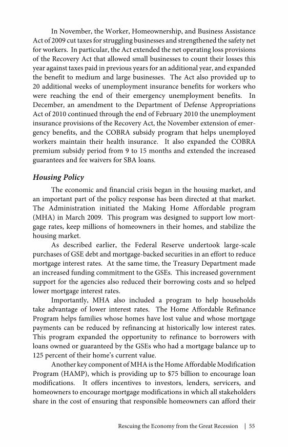
In November, the Worker, Homeownership, and Business AssistanceAct of 2009 cut taxes for struggling businesses and strengthened the safety netfor workers. In particular, the Act extended the net operating loss provisionsof the Recovery Act that allowed small businesses to count their losses thisyear against taxes paid in previous years for an additional year, and expandedthe benefit to medium and large businesses. The Act also provided up to20 additional weeks of unemployment insurance benefits for workers whowere reaching the end of their emergency unemployment benefits. InDecember, an amendment to the Department of Defense AppropriationsAct of 2010 continued through the end of February 2010 the unemploymentinsurance provisions of the Recovery Act, the November extension of emer-gency benefits, and the COBRA subsidy program that helps unemployedworkers maintain their health insurance. It also expanded the COBRApremium subsidy period from 9 to 15 months and extended the increasedguarantees and fee waivers for SBA loans.
Housing PolicyThe economic and financial crisis began in the housing market, and
an important part of the policy response has been directed at that market.The Administration initiated the Making Home Affordable program(MHA) in March 2009. This program was designed to support low mort-gage rates, keep millions of homeowners in their homes, and stabilize thehousing market.
As described earlier, the Federal Reserve undertook large-scalepurchases of GSE debt and mortgage-backed securities in an effort to reducemortgage interest rates. At the same time, the Treasury Department madean increased funding commitment to the GSEs. This increased governmentsupport for the agencies also reduced their borrowing costs and so helpedlower mortgage interest rates.
Importantly, MHA also included a program to help householdstake advantage of lower interest rates. The Home Affordable RefinanceProgram helps families whose homes have lost value and whose mortgagepayments can be reduced by refinancing at historically low interest rates.This program expanded the opportunity to refinance to borrowers withloans owned or guaranteed by the GSEs who had a mortgage balance up to125 percent of their home’s current value.
Another key component of MHA is the Home Affordable ModificationProgram (HAMP), which is providing up to $75 billion to encourage loanmodifications. It offers incentives to investors, lenders, servicers, andhomeowners to encourage mortgage modifications in which all stakeholdersshare in the cost of ensuring that responsible homeowners can afford their
56 | Chapter 2
monthly mortgage payments. To protect taxpayers, HAMP focuses onsound modifications. No payments are made by the government unlessthe modification lasts for at least three months, and all the payments aredesigned around the principle of “pay for success.” All parties have alignedincentives under the program to achieve successful modifications at anaffordable and sustainable level.
The Administration has supported additional programs to help thehousing sector. The Recovery Act included an $8,000 first-time homebuyer’scredit for home purchases made before December 1, 2009. As with tempo-rary investment incentives, this credit can help the economy by changingthe timing of decisions, bringing buyers into the housing market who werenot planning on becoming homeowners until after 2009 or were postponingtheir purchases in light of the distress in the market. In November, thiscredit was expanded and extended by the Workers, Homeownership, andBusiness Assistance Act of 2009.
TheRecoveryActalsogaveconsiderableresources to theNeighborhoodStabilization Program, a program administered by the Department ofHousing and Urban Development to stabilize communities that havesuffered from foreclosures and abandoned homes. The Administration alsoprovided assistance to state and local housing finance agencies and theirefforts to aid distressed homeowners, stimulate first-time home buying, andprovide affordable rental homes. These agencies had faced a significantliquidity crisis resulting from disruptions in financial markets.
The Effects of the Policies
The condition of the American economy has changed dramatically inthe past year. At the beginning of 2009, financial markets were functioningpoorly, house prices were plummeting, and output and employment werein freefall. Today, financial markets have stabilized and credit is starting toflow again, house prices have leveled off, output is growing, and the employ-ment situation is stabilizing. Because of the depth of the economy’s fall, weare a long way from full recovery, and significant challenges remain. But thetrajectory of the economy is vastly improved.
There is strong evidence that the policy response has been centralto this turnaround. The actions to stabilize credit markets have preventedfurther destructive failures of major financial institutions and helped main-tain lending in key areas. The housing and mortgage policies have kepthundreds of thousands of homeowners in their homes and brought mort-gage rates to historic lows. The speed of the economy’s change in directionhas been remarkable and matches up well with the timing of the fiscal
Rescuing the Economy from the Great Recession | 57
stimulus. And both direct estimates as well as the assessments of expertobservers underscore the crucial role played by the stimulus.
The Financial SectorGiven the powerful impact of the financial sector on the real economy,
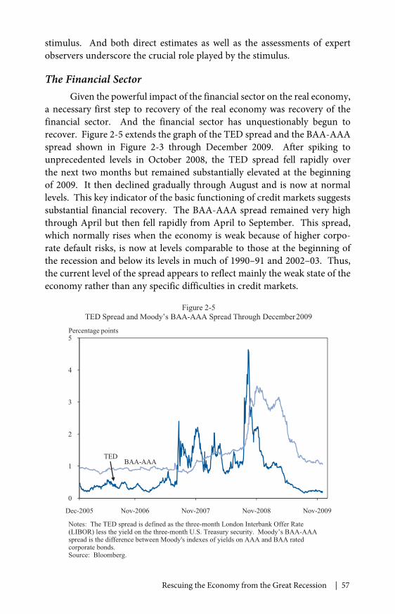
a necessary first step to recovery of the real economy was recovery of thefinancial sector. And the financial sector has unquestionably begun torecover. Figure 2-5 extends the graph of the TED spread and the BAA-AAAspread shown in Figure 2-3 through December 2009. After spiking tounprecedented levels in October 2008, the TED spread fell rapidly overthe next two months but remained substantially elevated at the beginningof 2009. It then declined gradually through August and is now at normallevels. This key indicator of the basic functioning of credit markets suggestssubstantial financial recovery. The BAA-AAA spread remained very highthrough April but then fell rapidly from April to September. This spread,which normally rises when the economy is weak because of higher corpo-rate default risks, is now at levels comparable to those at the beginning ofthe recession and below its levels in much of 1990–91 and 2002–03. Thus,the current level of the spread appears to reflect mainly the weak state of theeconomy rather than any specific difficulties in credit markets.
0
1
2
3
4
5
Dec-2005 Nov-2006 Nov-2007 Nov-2008 Nov-2009
Figure 2-5TED Spread and Moody’s BAA-AAA Spread Through December2009
Percentage points
BAA-AAATED
Notes: The TED spread is defined as the three-month London Interbank Offer Rate(LIBOR) less the yield on the three-month U.S. Treasury security. Moody’s BAA-AAAspread is the difference between Moody's indexes of yields on AAA and BAA ratedcorporate bonds.Source: Bloomberg.
58 | Chapter 2
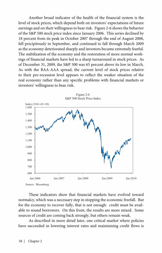
Another broad indicator of the health of the financial system is thelevel of stock prices, which depend both on investors’ expectations of futureearnings and on their willingness to bear risk. Figure 2-6 shows the behaviorof the S&P 500 stock price index since January 2006. This series declined by18 percent from its peak in October 2007 through the end of August 2008,fell precipitously in September, and continued to fall through March 2009as the economy deteriorated sharply and investors became extremely fearful.The stabilization of the economy and the restoration of more normal work-ings of financial markets have led to a sharp turnaround in stock prices. Asof December 31, 2009, the S&P 500 was 65 percent above its low in March.As with the BAA-AAA spread, the current level of stock prices relativeto their pre-recession level appears to reflect the weaker situation of thereal economy rather than any specific problems with financial markets orinvestors’ willingness to bear risk.
These indicators show that financial markets have evolved towardnormalcy, which was a necessary step in stopping the economic freefall. Butfor the economy to recover fully, that is not enough: credit must be avail-able to sound borrowers. On this front, the results are more mixed. Somesources of credit are coming back strongly, but others remain weak.
As described in more detail later, one critical market where policieshave succeeded in lowering interest rates and maintaining credit flows is
600
700
800
900
1,000
1,100
1,200
1,300
1,400
1,500
1,600
Jan-2006 Jan-2007 Jan-2008 Jan-2009 Jan-2010
Figure 2-6S&P 500 Stock Price Index
Index (1941-43=10)
Source: Bloomberg.
Rescuing the Economy from the Great Recession | 59
the mortgage market. Another market that has recovered substantially isthe market for commercial paper. In late 2008 and early 2009, this marketwas functioning in large part because of the direct intervention of theFederal Reserve. By mid-January, the Federal Reserve’s Commercial PaperFunding Facility (CPFF) was holding $350 billion of commercial paper. Ascredit conditions have stabilized, however, firms have been able to placetheir commercial paper privately on better terms than through the CPFF,and levels of commercial paper outstanding have remained stable evenas the Federal Reserve has reduced its holdings to less than $15 billion.Nonetheless, quantities of commercial paper outstanding remain well belowtheir pre-crisis levels.
Another crucial source of credit that has stabilized is the market forcorporate bonds. As risk spreads have fallen, corporations have found iteasier to obtain funding by issuing longer-term bonds than by issuing suchinstruments as commercial paper. As a result, corporate bond issuance, whichfell sharply in the second half of 2008, is now running above pre-crisis levels.
An important financial market development occurred in response tothe stress test conducted in the spring. This comprehensive review of thesoundness of the Nation’s 19 largest financial institutions, together with thepublic release of this information, strengthened private investors’ confi-dence in the institutions. Partly as a result, the institutions were able to raise$55 billion in private common equity, improving their capital positions andtheir ability to lend.
The fact that financial institutions are increasingly able to raise privatecapital is reducing their need to rely on public capital. Only $7 billion ofTARP funds have been extended to banks since January 20, 2009. Manyfinancial institutions have repaid their TARP funds, and the expected costof the program to the government has been revised down by approximately$200 billion since August 2009.
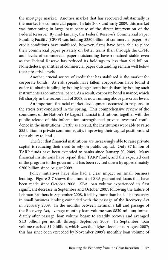
Policy initiatives have also had a clear impact on small businesslending. Figure 2-7 shows the amount of SBA-guaranteed loans that havebeen made since October 2006. SBA loan volume experienced its firstsignificant decrease in September and October 2007; following the failure ofLehman Brothers in September 2008, it fell by more than half. The recoveryin small business lending coincided with the passage of the Recovery Actin February 2009. In the months between Lehman’s fall and passage ofthe Recovery Act, average monthly loan volume was $830 million; imme-diately after passage, loan volume began to steadily recover and averaged$1.3 billion per month through September 2009. In September, loanvolume reached $1.9 billion, which was the highest level since August 2007;this has since been exceeded by November 2009’s monthly loan volume of
60 | Chapter 2
$2.2 billion. In total, between February and December 2009 the SBAguaranteed nearly $15 billion in small business lending.
Nonetheless, overall credit conditions have not returned to normal.Many small business owners report continued difficulties in obtainingcredit. In addition, the severity of the downturn is leading to elevated ratesof failure of small banks, potentially disrupting their lending to small busi-nesses and households. The market for asset-backed securities is also farfrom fully recovered. As a result, it is often hard for banks and other lendersto package and sell their loans, which forces them to hold a greater fractionof the loans they originate and thus limits their ability to lend.
One important source of data on credit availability is the FederalReserve’s Senior Loan Officer Opinion Survey on Bank Lending Practices.The survey, conducted every three months, examines whether banksare tightening lending standards, loosening them, or keeping them basi-cally unchanged. The October 2008 survey found that the overwhelmingmajority of banks were tightening standards. This fraction has declinedsteadily, and by October 2009 less than 20 percent were reporting that theywere tightening standards for commercial and industrial loans, though nonereported loosening standards. Thus, credit conditions remain tight.
HousingAs described earlier, policymakers have taken unprecedented actions
to maintain mortgage lending. One result has been a major shift in the
0
500
1,000
1,500
2,000
2,500
Oct-2006 Apr-2007 Oct-2007 Apr-2008 Oct-2008 Apr-2009 Oct-2009
Figure 2-7
Monthly Gross SBA 7(a) and 504 Loan Approvals
Millions of dollars
Before ARRA After ARRA
10/08-2/09 average$830 million
3/09-12/09 average$1,380million
Source: Unpublished monthly data provided by the Small Business Administration.
Rescuing the Economy from the Great Recession | 61
composition of mortgage finance. In 2006, private institutions provided60 percent of liquidity while the GSEs, the Federal Housing Agency (FHA),and the Veterans Administration (VA) provided the remaining 40 percent.As home prices began to decline nationally in 2007, private financing formortgages began to dry up. As of November 2009, the mortgages guar-anteed by the GSEs, FHA, and the VA accounted for nearly all mortgageoriginations. About 22 percent of mortgage originations are guaranteedby FHA or VA, up from less than 3 percent in 2006. About 75 percentof mortgage originations are guaranteed by the GSEs, up from less than40 percent in 2006.
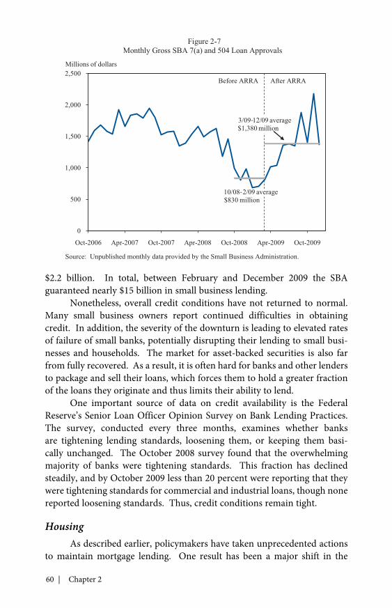
As Figure 2-8 shows, mortgage rates fell to historic lows in 2009—consistent with the government’s increased funding commitment to FannieMae and Freddie Mac and the Federal Reserve’s purchases of mortgage-backed securities. These low mortgage rates support home prices and thusbenefit all homeowners. More directly, households that have refinancedtheir mortgages at the lower rates have obtained considerable savings. Thesesavings have effects similar to tax cuts, improving households’ financialpositions and encouraging spending on other goods. With the help of theHome Affordable Refinance Program, approximately 3 million borrowershave refinanced, putting more than $6 billion of purchasing power at anannual rate into the hands of households.
0
2
4
6
8
10
12
14
16
18
20
Apr-1971 Apr-1977 Apr-1983 Mar-1989 Mar-1995 Mar-2001 Mar-2007
Figure 2-830-Year Fixed Rate Mortgage Rate
Percent
Note: Contract interest rate for first mortgages.Source: Freddie Mac, Primary Mortgage Market Survey.
62 | Chapter 2
In addition, the Home Affordable Modification Program has beensuccessful in encouraging mortgage modifications. When the program waslaunched, the Administration estimated that it could offer help to as manyas 3 million to 4 million borrowers through the end of 2012. On October8, 2009, the Administration announced that servicers had begun more than500,000 trial modifications, nearly a month ahead of the original goal. Asof November, the monthly pace of trial modifications exceeded the monthlypace of completed foreclosures. Of course, not all trial modifications willbecome permanent, but the Administration is making every effort to ensurethat as many sound modifications as possible do.
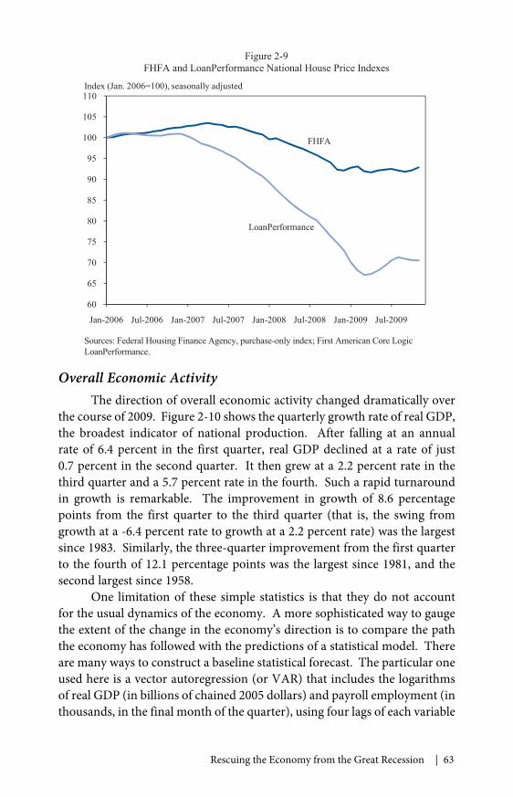
One important result of the policies aimed at the housing marketand of the broader policies to support the economy is that the housingmarket appears to have stabilized. National home price indexes havebeen relatively steady for the past several months, as shown in Figure 2-9.The Federal Housing Finance Agency purchase-only house price index,which is constructed using only conforming mortgages (that is, mortgageseligible for purchase by the GSEs), has changed little since late 2008. TheLoanPerformance house price index, another closely watched measure thatuses conforming and nonconforming mortgages with coverage of repeatsales transactions for more than 85 percent of the population, rose 6 percentbetween March and August 2009 before declining slightly in recent months.In addition, the pace of sales of existing single-family homes has increasedsubstantially. Sales in the fourth quarter of 2009 were 29 percent abovetheir low in the first quarter of 2009 and comparable to levels in the first halfof 2007.
Finally, there are signs of renewed building activity. After falling81 percent from their peak in September 2005 to their low in January 2009,single-family housing permits (a leading indicator of housing construc-tion) rose 49 percent through December 2009. Similarly, after falling for14 consecutive quarters, the residential investment component of real GDProse in the third and fourth quarters of 2009.
Inventories of vacant homes for sale remain at high levels, and manyvacant homes are being held off the market and will likely be put up forsale as home prices increase. This overhang may lead to some additionalprice declines, although prices are unlikely to fall at the same rate as theydid during the crisis. Thus, the recovery of the housing sector is likely to beslow. Of course, we should neither expect nor want the housing market toreturn to its pre-crisis condition. In the long run, as discussed in more detailin Chapter 4, neither the extraordinarily high levels of housing constructionand price appreciation before the crisis nor the extraordinarily low levels ofconstruction and the rapid price declines during the crisis are sustainable.
Rescuing the Economy from the Great Recession | 63
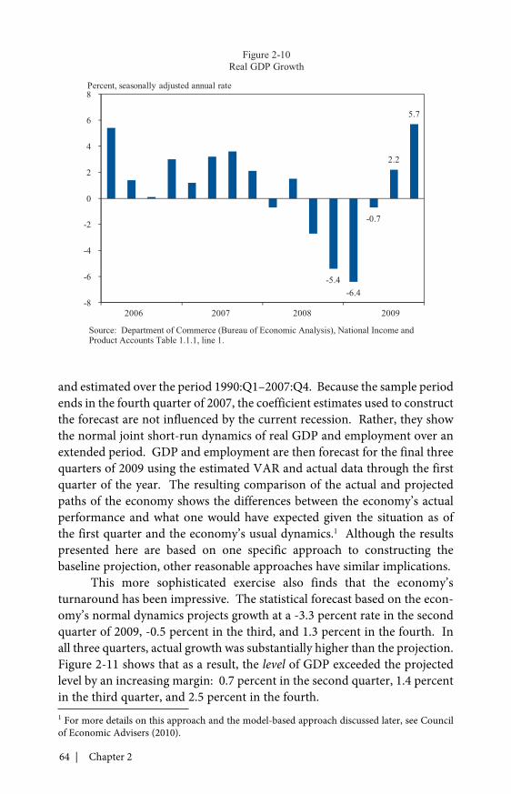
Overall Economic ActivityThe direction of overall economic activity changed dramatically over
the course of 2009. Figure 2-10 shows the quarterly growth rate of real GDP,the broadest indicator of national production. After falling at an annualrate of 6.4 percent in the first quarter, real GDP declined at a rate of just0.7 percent in the second quarter. It then grew at a 2.2 percent rate in thethird quarter and a 5.7 percent rate in the fourth. Such a rapid turnaroundin growth is remarkable. The improvement in growth of 8.6 percentagepoints from the first quarter to the third quarter (that is, the swing fromgrowth at a -6.4 percent rate to growth at a 2.2 percent rate) was the largestsince 1983. Similarly, the three-quarter improvement from the first quarterto the fourth of 12.1 percentage points was the largest since 1981, and thesecond largest since 1958.
One limitation of these simple statistics is that they do not accountfor the usual dynamics of the economy. A more sophisticated way to gaugethe extent of the change in the economy’s direction is to compare the paththe economy has followed with the predictions of a statistical model. Thereare many ways to construct a baseline statistical forecast. The particular oneused here is a vector autoregression (or VAR) that includes the logarithmsof real GDP (in billions of chained 2005 dollars) and payroll employment (inthousands, in the final month of the quarter), using four lags of each variable
60
65
70
75
80
85
90
95
100
105
110
Jan-2006 Jul-2006 Jan-2007 Jul-2007 Jan-2008 Jul-2008 Jan-2009 Jul-2009
Figure 2-9FHFA and LoanPerformance National House Price Indexes
Index (Jan. 2006=100), seasonally adjusted
LoanPerformance
FHFA
Sources: Federal Housing Finance Agency, purchase-only index; First American Core LogicLoanPerformance.
64 | Chapter 2
and estimated over the period 1990:Q1–2007:Q4. Because the sample periodends in the fourth quarter of 2007, the coefficient estimates used to constructthe forecast are not influenced by the current recession. Rather, they showthe normal joint short-run dynamics of real GDP and employment over anextended period. GDP and employment are then forecast for the final threequarters of 2009 using the estimated VAR and actual data through the firstquarter of the year. The resulting comparison of the actual and projectedpaths of the economy shows the differences between the economy’s actualperformance and what one would have expected given the situation as ofthe first quarter and the economy’s usual dynamics.1 Although the resultspresented here are based on one specific approach to constructing thebaseline projection, other reasonable approaches have similar implications.
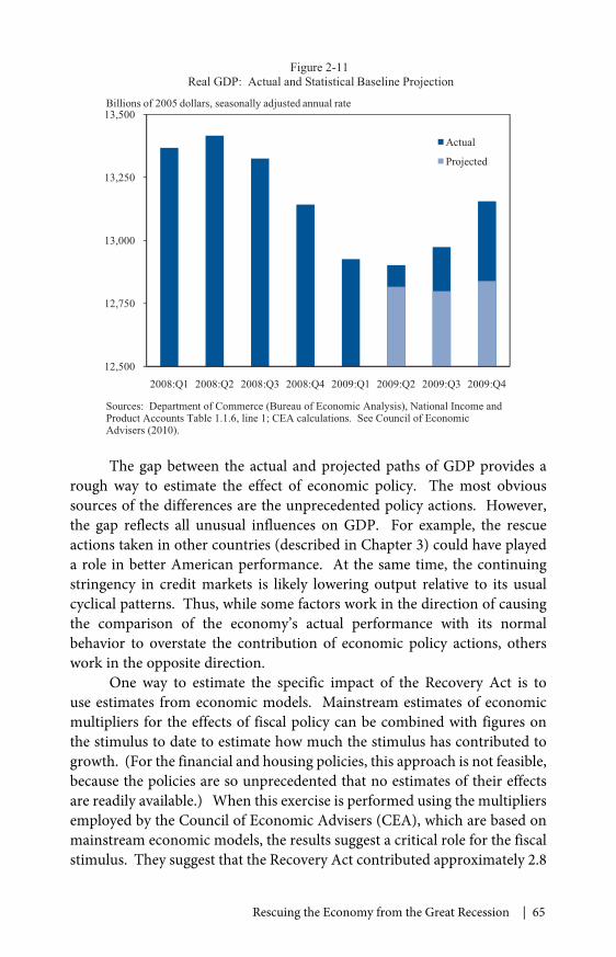
This more sophisticated exercise also finds that the economy’sturnaround has been impressive. The statistical forecast based on the econ-omy’s normal dynamics projects growth at a -3.3 percent rate in the secondquarter of 2009, -0.5 percent in the third, and 1.3 percent in the fourth. Inall three quarters, actual growth was substantially higher than the projection.Figure 2-11 shows that as a result, the level of GDP exceeded the projectedlevel by an increasing margin: 0.7 percent in the second quarter, 1.4 percentin the third quarter, and 2.5 percent in the fourth.1 For more details on this approach and the model-based approach discussed later, see Councilof Economic Advisers (2010).
-5.4-6.4
-0.7
2.2
5.7
-8
-6
-4
-2
0
2
4
6
8
Figure 2-10Real GDP Growth
Percent, seasonally adjusted annual rate
2006 2007 2008 2009
Source: Department of Commerce (Bureau of Economic Analysis), National Income andProduct Accounts Table 1.1.1, line 1.
Rescuing the Economy from the Great Recession | 65
The gap between the actual and projected paths of GDP provides arough way to estimate the effect of economic policy. The most obvioussources of the differences are the unprecedented policy actions. However,the gap reflects all unusual influences on GDP. For example, the rescueactions taken in other countries (described in Chapter 3) could have playeda role in better American performance. At the same time, the continuingstringency in credit markets is likely lowering output relative to its usualcyclical patterns. Thus, while some factors work in the direction of causingthe comparison of the economy’s actual performance with its normalbehavior to overstate the contribution of economic policy actions, otherswork in the opposite direction.
One way to estimate the specific impact of the Recovery Act is touse estimates from economic models. Mainstream estimates of economicmultipliers for the effects of fiscal policy can be combined with figures onthe stimulus to date to estimate how much the stimulus has contributed togrowth. (For the financial and housing policies, this approach is not feasible,because the policies are so unprecedented that no estimates of their effectsare readily available.) When this exercise is performed using the multipliersemployed by the Council of Economic Advisers (CEA), which are based onmainstream economic models, the results suggest a critical role for the fiscalstimulus. They suggest that the Recovery Act contributed approximately 2.8
12,500
12,750
13,000
13,250
13,500
2008:Q1 2008:Q2 2008:Q3 2008:Q4 2009:Q1 2009:Q2 2009:Q3 2009:Q4
Actual
Projected
Figure 2-11Real GDP: Actual and Statistical Baseline Projection
Billions of 2005 dollars, seasonally adjusted annual rate
Sources: Department of Commerce (Bureau of Economic Analysis), National Income andProduct Accounts Table 1.1.6, line 1; CEA calculations. See Council of EconomicAdvisers (2010).
66 | Chapter 2
percentage points to growth in the second quarter, 3.9 percentage points inthe third, and 1.8 percentage points in the fourth. As a result, this approachsuggests that the level of GDP in the fourth quarter was slightly more than2 percent higher than it would have been in the absence of the stimulus.
Knowledgeable outside observers agree that the Recovery Act hasincreased output substantially relative to what it otherwise would have been.For example, in November 2009, CBO estimated that the Act had raised thelevel of output in the third quarter by between 1.2 and 3.2 percent relative tothe no-stimulus baseline (Congressional Budget Office 2009a). Private fore-casters also generally estimate that the Act has raised output substantially.
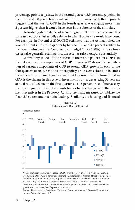
A final way to look for the effects of the rescue policies on GDP is inthe behavior of the components of GDP. Figure 2-12 shows the contribu-tion of various components of GDP to overall GDP growth in each of thefour quarters of 2009. One area where policy’s role seems clear is in businessinvestment in equipment and software. A key source of the turnaround inGDP is the change in this type of investment from a devastating 36 percentannual rate of decline in the first quarter to a 13 percent rate of increase bythe fourth quarter. Two likely contributors to this change were the invest-ment incentives in the Recovery Act and the many measures to stabilize thefinancial system and maintain lending. Similarly, the housing and financial
-4
-3
-2
-1
0
1
2
3
4
5
6
2009:Q1
2009:Q2
2009:Q3
2009:Q4
Figure 2-12Contributions to Real GDP Growth
Percentage points
PCE Nonres.Struct.
Res.Fixed I
InventoryI
Fed.Gov’t
S&LGov’t
NetExports
Equip. I
Notes: Bars sum to quarterly change in GDP growth (-6.4% in Q1; -0.7% in Q2; 2.2% inQ3; 5.7% in Q4). PCE is personal consumption expenditures; Nonres. Struct. is nonresiden-tial fixed investment in structures; Equip I. is nonresidential fixed investment in equipmentand software; Res. Fixed I is residential fixed investment; Inventory I is inventoryinvestment; Federal Gov’t is Federal Government purchases; S&L Gov’t is state and localgovernment purchases; Net Exports is net exports.Source: Department of Commerce (Bureau of Economic Analysis), National Income andProduct Accounts Table 1.1.2.
Rescuing the Economy from the Great Recession | 67
market policies were surely important to the swing in the growth of residen-tial investment from a 38 percent annual rate of decline in the first quarterto increases in the third and fourth quarters.
Two other components showing evidence of the policies’ effectsare personal consumption expenditures and state and local governmentpurchases. The Making Work Pay tax credit and the aid to individualsdirectly affected by the recession meant that households did not have to cuttheir consumption spending as much as they otherwise would have, andthe Cash for Clunkers program provided important incentives for motorvehicle purchases in the third quarter. Consumption was little changed inthe first two quarters of 2009 and then rose at a healthy 2.8 percent annualrate in the third quarter—driven in considerable part by a 44 percent rate ofincrease in purchases of motor vehicles and parts—and at a 2.0 percent ratein the fourth quarter. And, despite the dire budgetary situations of state andlocal governments, their purchases rose at the fastest pace in more than fiveyears in the second quarter and were basically stable in the third and fourthquarters. This stability almost surely could not have occurred in the absenceof the fiscal relief to the states.
The figure also shows the large role of inventory investment inmagnifying macroeconomic fluctuations. When the economy goes intoa recession, firms want to cut their inventories. As a result, inventoryinvestment moves from its usual slightly positive level to sharply negative,contributing to the fall in output. Then, as firms moderate their inventoryreductions, inventory investment rises—that is, becomes less negative—contributing to the recovery of output.
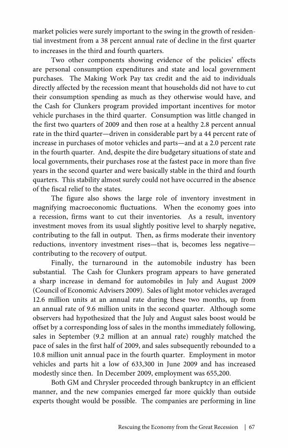
Finally, the turnaround in the automobile industry has beensubstantial. The Cash for Clunkers program appears to have generateda sharp increase in demand for automobiles in July and August 2009(Council of Economic Advisers 2009). Sales of light motor vehicles averaged12.6 million units at an annual rate during these two months, up froman annual rate of 9.6 million units in the second quarter. Although someobservers had hypothesized that the July and August sales boost would beoffset by a corresponding loss of sales in the months immediately following,sales in September (9.2 million at an annual rate) roughly matched thepace of sales in the first half of 2009, and sales subsequently rebounded to a10.8 million unit annual pace in the fourth quarter. Employment in motorvehicles and parts hit a low of 633,300 in June 2009 and has increasedmodestly since then. In December 2009, employment was 655,200.
Both GM and Chrysler proceeded through bankruptcy in an efficientmanner, and the new companies emerged far more quickly than outsideexperts thought would be possible. The companies are performing in line
68 | Chapter 2
with their restructuring plans, and in November 2009, GM announced itsintention to begin repaying the Federal Government earlier than originallyexpected. It made a first payment of $1 billion in December.
The Labor MarketThe ultimate goal of the economic stabilization and recovery
policies is to provide a job for every American who seeks one. The recession’simpact on the labor market has been severe: employment in December 2009was 7.2 million below its peak level two years earlier, and the unemploy-ment rate was 10 percent. Moreover, although real GDP has begun to grow,employment losses are continuing.
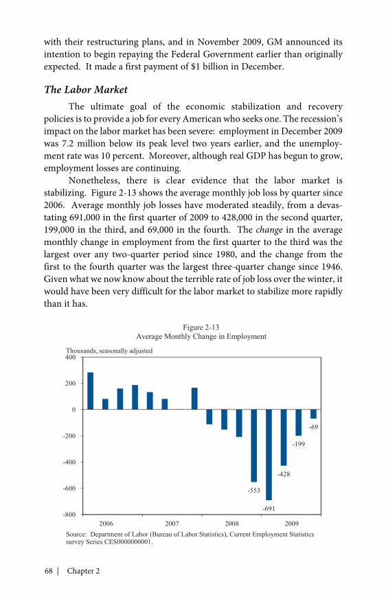
Nonetheless, there is clear evidence that the labor market isstabilizing. Figure 2-13 shows the average monthly job loss by quarter since2006. Average monthly job losses have moderated steadily, from a devas-tating 691,000 in the first quarter of 2009 to 428,000 in the second quarter,199,000 in the third, and 69,000 in the fourth. The change in the averagemonthly change in employment from the first quarter to the third was thelargest over any two-quarter period since 1980, and the change from thefirst to the fourth quarter was the largest three-quarter change since 1946.Given what we now know about the terrible rate of job loss over the winter, itwould have been very difficult for the labor market to stabilize more rapidlythan it has.
-553
-691
-428
-199
-69
-800
-600
-400
-200
0
200
400
Figure 2-13Average Monthly Change in Employment
Thousands, seasonally adjusted
2006 2007 2008 2009Source: Department of Labor (Bureau of Labor Statistics), Current Employment Statisticssurvey Series CES0000000001.
Rescuing the Economy from the Great Recession | 69
One can again use the VAR described earlier to obtain a morerefined estimate of how the behavior of employment has differed from itsusual pattern. This statistical procedure implies that given the economy’sbehavior through the first quarter of 2009 and its usual dynamics, one wouldhave expected job losses of about 597,000 per month in the second quarter,513,000 in the third quarter, and 379,000 in the fourth. Thus, actual employ-ment as of the middle of the second quarter (May) was approximately300,000 higher than one would have projected given the normal behaviorof the economy; as of the middle of the third quarter (August), it was about1.1 million higher; and as of the middle of the fourth quarter (November), itwas about 2.1 million higher. As with the behavior of GDP, the portion of thisdifference that is attributable to the Recovery Act and other policies cannotbe isolated from the portion resulting from other factors. But again, thedifference could either understate or overstate the policies’ contributions.
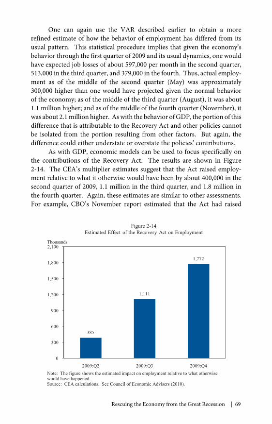
As with GDP, economic models can be used to focus specifically onthe contributions of the Recovery Act. The results are shown in Figure2-14. The CEA’s multiplier estimates suggest that the Act raised employ-ment relative to what it otherwise would have been by about 400,000 in thesecond quarter of 2009, 1.1 million in the third quarter, and 1.8 million inthe fourth quarter. Again, these estimates are similar to other assessments.For example, CBO’s November report estimated that the Act had raised
385
1,111
1,772
0
300
600
900
1,200
1,500
1,800
2,100
2009:Q2 2009:Q3 2009:Q4
Figure 2-14Estimated Effect of the Recovery Act on Employment
Thousands
Note: The figure shows the estimated impact on employment relative to what otherwisewould have happened.Source: CEA calculations. See Council of Economic Advisers (2010).
70 | Chapter 2
employment in the third quarter by between 0.6 million and 1.6 million,relative to what otherwise would have happened.
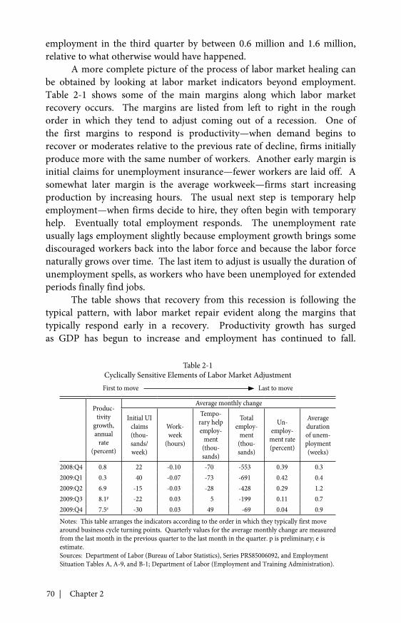
A more complete picture of the process of labor market healing canbe obtained by looking at labor market indicators beyond employment.Table 2-1 shows some of the main margins along which labor marketrecovery occurs. The margins are listed from left to right in the roughorder in which they tend to adjust coming out of a recession. One ofthe first margins to respond is productivity—when demand begins torecover or moderates relative to the previous rate of decline, firms initiallyproduce more with the same number of workers. Another early margin isinitial claims for unemployment insurance—fewer workers are laid off. Asomewhat later margin is the average workweek—firms start increasingproduction by increasing hours. The usual next step is temporary helpemployment—when firms decide to hire, they often begin with temporaryhelp. Eventually total employment responds. The unemployment rateusually lags employment slightly because employment growth brings somediscouraged workers back into the labor force and because the labor forcenaturally grows over time. The last item to adjust is usually the duration ofunemployment spells, as workers who have been unemployed for extendedperiods finally find jobs.
The table shows that recovery from this recession is following thetypical pattern, with labor market repair evident along the margins thattypically respond early in a recovery. Productivity growth has surgedas GDP has begun to increase and employment has continued to fall.
Table 2-1Cyclically Sensitive Elements of Labor Market AdjustmentFirst to move Last to move
Produc-tivity
growth,annual
rate(percent)
Average monthly change
Initial UIclaims(thou-sands/week)
Work-week
(hours)
Tempo-rary helpemploy-
ment(thou-sands)
Totalemploy-
ment(thou-sands)
Un-employ-
ment rate(percent)
Averagedurationof unem-ployment(weeks)
2008:Q4 0.8 22 -0.10 -70 -553 0.39 0.32009:Q1 0.3 40 -0.07 -73 -691 0.42 0.42009:Q2 6.9 -15 -0.03 -28 -428 0.29 1.22009:Q3 8.1p -22 0.03 5 -199 0.11 0.72009:Q4 7.5e -30 0.03 49 -69 0.04 0.9Notes: This table arranges the indicators according to the order in which they typically first movearound business cycle turning points. Quarterly values for the average monthly change are measuredfrom the last month in the previous quarter to the last month in the quarter. p is preliminary; e isestimate.Sources: Department of Labor (Bureau of Labor Statistics), Series PRS85006092, and EmploymentSituation Tables A, A-9, and B-1; Department of Labor (Employment and Training Administration).
Rescuing the Economy from the Great Recession | 71
Initial unemployment insurance claims, which rose precipitously earlierin the recession, have begun to decline at an increasing rate. Likewise, theworkweek has gone from shortening to lengthening, albeit slowly. Temporaryhelp employment has changed from extreme declines to substantial increases.So far, total employment has shown a greatly moderating decline but has notyet risen. The pace of increase in the unemployment rate has slowed notice-ably, but the unemployment rate has not yet fallen on a quarterly basis.Finally, increases in the duration of unemployment have not yet begun tomoderate noticeably.
These data suggest that the labor market is beginning to move inthe right direction, but much work remains to be done. The country isnot yet seeing the substantial rises in total employment and declines in theunemployment rate that are the ultimate hallmark of robust labor marketimprovement. And, of course, even once all the indicators are movingsolidly in the right direction, the labor market will still have a long way to gobefore it is fully recovered.
Signs of healing are also beginning to appear in the industrialcomposition of the stabilization of the labor market. Figure 2-15 shows theaverage monthly change in each of eight sectors in each of the four quartersof 2009. As one would expect of the beginnings of a recovery from a severe
-240
-190
-140
-90
-40
10
60
110
160
2009:Q1
2009:Q2
2009:Q3
2009:Q4
Figure 2-15Contributions to the Change in Employment
Thousands, average monthly change from end of quarter to end of quarter
Con-struct.
Mfg. Trade Prof. &Bus. Serv.
Edu. &Health
FederalGov’t
S&LGov’t
Other
Notes: Bars sum to average monthly change in quarter (-691,000 in Q1; -428,000 in Q2;-199,000 in Q3; -69,000 in Q4). Construct. is construction; Mfg. is manufacturing; Trade iswholesale and retail trade, transportation, and utilities; Prof. & Bus. Serv. is professional andbusiness services; Edu. & Health is education and health; Federal Gov’t is FederalGovernment; S&L Gov’t is state and local government.Source: Department of Labor (Bureau of Labor Statistics), Employment Situation Table B-1.
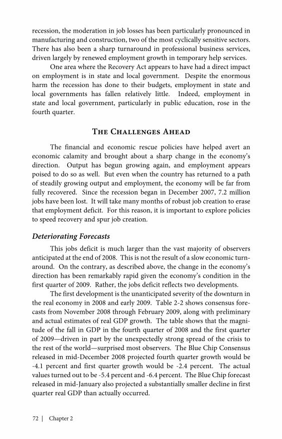
72 | Chapter 2
recession, the moderation in job losses has been particularly pronounced inmanufacturing and construction, two of the most cyclically sensitive sectors.There has also been a sharp turnaround in professional business services,driven largely by renewed employment growth in temporary help services.
One area where the Recovery Act appears to have had a direct impacton employment is in state and local government. Despite the enormousharm the recession has done to their budgets, employment in state andlocal governments has fallen relatively little. Indeed, employment instate and local government, particularly in public education, rose in thefourth quarter.
The Challenges Ahead
The financial and economic rescue policies have helped avert aneconomic calamity and brought about a sharp change in the economy’sdirection. Output has begun growing again, and employment appearspoised to do so as well. But even when the country has returned to a pathof steadily growing output and employment, the economy will be far fromfully recovered. Since the recession began in December 2007, 7.2 millionjobs have been lost. It will take many months of robust job creation to erasethat employment deficit. For this reason, it is important to explore policiesto speed recovery and spur job creation.
Deteriorating ForecastsThis jobs deficit is much larger than the vast majority of observers
anticipated at the end of 2008. This is not the result of a slow economic turn-around. On the contrary, as described above, the change in the economy’sdirection has been remarkably rapid given the economy’s condition in thefirst quarter of 2009. Rather, the jobs deficit reflects two developments.
The first development is the unanticipated severity of the downturn inthe real economy in 2008 and early 2009. Table 2-2 shows consensus fore-casts from November 2008 through February 2009, along with preliminaryand actual estimates of real GDP growth. The table shows that the magni-tude of the fall in GDP in the fourth quarter of 2008 and the first quarterof 2009—driven in part by the unexpectedly strong spread of the crisis tothe rest of the world—surprised most observers. The Blue Chip Consensusreleased in mid-December 2008 projected fourth quarter growth would be-4.1 percent and first quarter growth would be -2.4 percent. The actualvalues turned out to be -5.4 percent and -6.4 percent. The Blue Chip forecastreleased in mid-January also projected a substantially smaller decline in firstquarter real GDP than actually occurred.
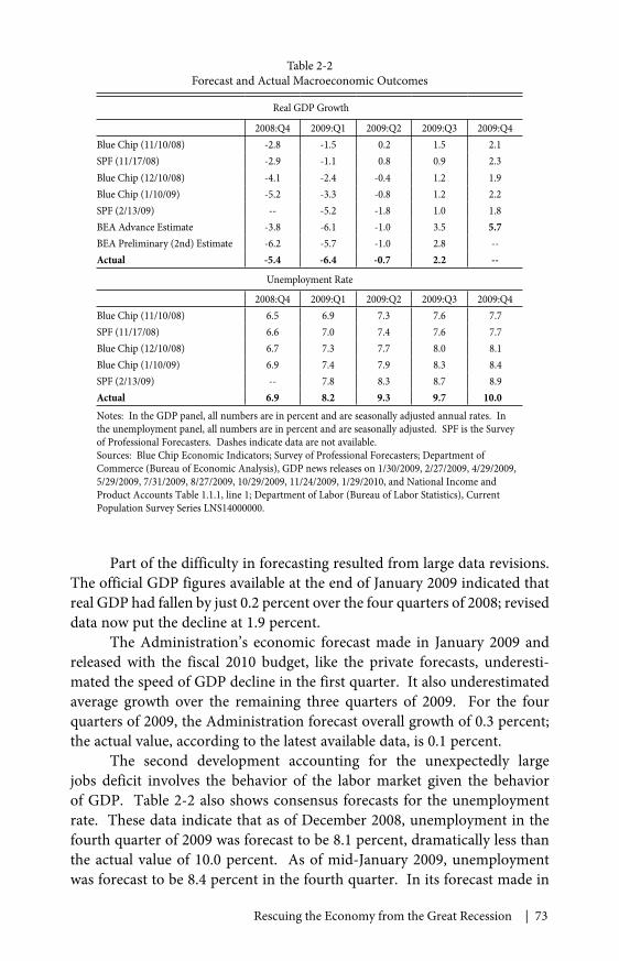
Rescuing the Economy from the Great Recession | 73
Part of the difficulty in forecasting resulted from large data revisions.The official GDP figures available at the end of January 2009 indicated thatreal GDP had fallen by just 0.2 percent over the four quarters of 2008; reviseddata now put the decline at 1.9 percent.
The Administration’s economic forecast made in January 2009 andreleased with the fiscal 2010 budget, like the private forecasts, underesti-mated the speed of GDP decline in the first quarter. It also underestimatedaverage growth over the remaining three quarters of 2009. For the fourquarters of 2009, the Administration forecast overall growth of 0.3 percent;the actual value, according to the latest available data, is 0.1 percent.
The second development accounting for the unexpectedly largejobs deficit involves the behavior of the labor market given the behaviorof GDP. Table 2-2 also shows consensus forecasts for the unemploymentrate. These data indicate that as of December 2008, unemployment in thefourth quarter of 2009 was forecast to be 8.1 percent, dramatically less thanthe actual value of 10.0 percent. As of mid-January 2009, unemploymentwas forecast to be 8.4 percent in the fourth quarter. In its forecast made in
Table 2-2Forecast and Actual Macroeconomic Outcomes
Real GDP Growth
2008:Q4 2009:Q1 2009:Q2 2009:Q3 2009:Q4Blue Chip (11/10/08) -2.8 -1.5 0.2 1.5 2.1SPF (11/17/08) -2.9 -1.1 0.8 0.9 2.3Blue Chip (12/10/08) -4.1 -2.4 -0.4 1.2 1.9Blue Chip (1/10/09) -5.2 -3.3 -0.8 1.2 2.2SPF (2/13/09) -- -5.2 -1.8 1.0 1.8BEA Advance Estimate -3.8 -6.1 -1.0 3.5 5.7BEA Preliminary (2nd) Estimate -6.2 -5.7 -1.0 2.8 --Actual -5.4 -6.4 -0.7 2.2 --
Unemployment Rate
2008:Q4 2009:Q1 2009:Q2 2009:Q3 2009:Q4Blue Chip (11/10/08) 6.5 6.9 7.3 7.6 7.7SPF (11/17/08) 6.6 7.0 7.4 7.6 7.7Blue Chip (12/10/08) 6.7 7.3 7.7 8.0 8.1Blue Chip (1/10/09) 6.9 7.4 7.9 8.3 8.4SPF (2/13/09) -- 7.8 8.3 8.7 8.9Actual 6.9 8.2 9.3 9.7 10.0Notes: In the GDP panel, all numbers are in percent and are seasonally adjusted annual rates. Inthe unemployment panel, all numbers are in percent and are seasonally adjusted. SPF is the Surveyof Professional Forecasters. Dashes indicate data are not available.Sources: Blue Chip Economic Indicators; Survey of Professional Forecasters; Department ofCommerce (Bureau of Economic Analysis), GDP news releases on 1/30/2009, 2/27/2009, 4/29/2009,5/29/2009, 7/31/2009, 8/27/2009, 10/29/2009, 11/24/2009, 1/29/2010, and National Income andProduct Accounts Table 1.1.1, line 1; Department of Labor (Bureau of Labor Statistics), CurrentPopulation Survey Series LNS14000000.
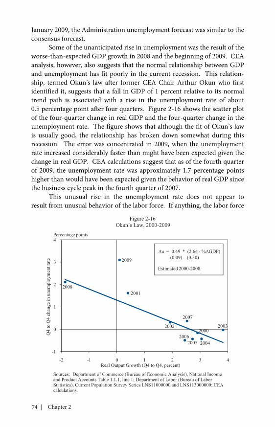
74 | Chapter 2
January 2009, the Administration unemployment forecast was similar to theconsensus forecast.
Some of the unanticipated rise in unemployment was the result of theworse-than-expected GDP growth in 2008 and the beginning of 2009. CEAanalysis, however, also suggests that the normal relationship between GDPand unemployment has fit poorly in the current recession. This relation-ship, termed Okun’s law after former CEA Chair Arthur Okun who firstidentified it, suggests that a fall in GDP of 1 percent relative to its normaltrend path is associated with a rise in the unemployment rate of about0.5 percentage point after four quarters. Figure 2-16 shows the scatter plotof the four-quarter change in real GDP and the four-quarter change in theunemployment rate. The figure shows that although the fit of Okun’s lawis usually good, the relationship has broken down somewhat during thisrecession. The error was concentrated in 2009, when the unemploymentrate increased considerably faster than might have been expected given thechange in real GDP. CEA calculations suggest that as of the fourth quarterof 2009, the unemployment rate was approximately 1.7 percentage pointshigher than would have been expected given the behavior of real GDP sincethe business cycle peak in the fourth quarter of 2007.
This unusual rise in the unemployment rate does not appear toresult from unusual behavior of the labor force. If anything, the labor force
2000
2001
2002 2003
200420052006
2007
2008
2009
-1
0
1
2
3
4
-2 -1 0 1 2 3 4
Q4
toQ
4ch
ange
inun
empl
oym
entr
ate
Figure 2-16Okun’s Law, 2000-2009
Percentage points
ru = 0.49 * (2.64 - %rGDP)(0.09) (0.30)
Estimated 2000-2008.
Real Output Growth (Q4 to Q4, percent)
Sources: Department of Commerce (Bureau of Economic Analysis), National Incomeand Product Accounts Table 1.1.1, line 1; Department of Labor (Bureau of LaborStatistics), Current Population Survey Series LNS11000000 and LNS113000000; CEAcalculations.
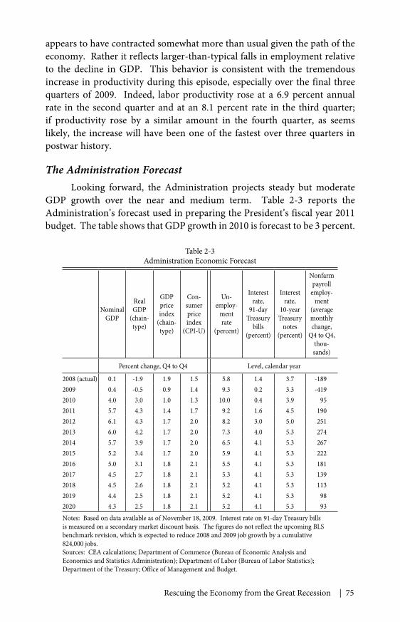
Rescuing the Economy from the Great Recession | 75
appears to have contracted somewhat more than usual given the path of theeconomy. Rather it reflects larger-than-typical falls in employment relativeto the decline in GDP. This behavior is consistent with the tremendousincrease in productivity during this episode, especially over the final threequarters of 2009. Indeed, labor productivity rose at a 6.9 percent annualrate in the second quarter and at an 8.1 percent rate in the third quarter;if productivity rose by a similar amount in the fourth quarter, as seemslikely, the increase will have been one of the fastest over three quarters inpostwar history.
The Administration ForecastLooking forward, the Administration projects steady but moderate
GDP growth over the near and medium term. Table 2-3 reports theAdministration’s forecast used in preparing the President’s fiscal year 2011budget. The table shows that GDP growth in 2010 is forecast to be 3 percent.
Table 2-3Administration Economic Forecast
NominalGDP
RealGDP
(chain-type)
GDPpriceindex
(chain-type)
Con-sumerpriceindex
(CPI-U)
Un-employ-
mentrate
(percent)
Interestrate,
91-dayTreasury
bills(percent)
Interestrate,
10-yearTreasury
notes(percent)
Nonfarmpayroll
employ-ment
(averagemonthlychange,
Q4 to Q4,thou-sands)
Percent change, Q4 to Q4 Level, calendar year
2008 (actual) 0.1 -1.9 1.9 1.5 5.8 1.4 3.7 -1892009 0.4 -0.5 0.9 1.4 9.3 0.2 3.3 -4192010 4.0 3.0 1.0 1.3 10.0 0.4 3.9 952011 5.7 4.3 1.4 1.7 9.2 1.6 4.5 1902012 6.1 4.3 1.7 2.0 8.2 3.0 5.0 2512013 6.0 4.2 1.7 2.0 7.3 4.0 5.3 2742014 5.7 3.9 1.7 2.0 6.5 4.1 5.3 2672015 5.2 3.4 1.7 2.0 5.9 4.1 5.3 2222016 5.0 3.1 1.8 2.1 5.5 4.1 5.3 1812017 4.5 2.7 1.8 2.1 5.3 4.1 5.3 1392018 4.5 2.6 1.8 2.1 5.2 4.1 5.3 1132019 4.4 2.5 1.8 2.1 5.2 4.1 5.3 982020 4.3 2.5 1.8 2.1 5.2 4.1 5.3 93Notes: Based on data available as of November 18, 2009. Interest rate on 91-day Treasury billsis measured on a secondary market discount basis. The figures do not reflect the upcoming BLSbenchmark revision, which is expected to reduce 2008 and 2009 job growth by a cumulative824,000 jobs.Sources: CEA calculations; Department of Commerce (Bureau of Economic Analysis andEconomics and Statistics Administration); Department of Labor (Bureau of Labor Statistics);Department of the Treasury; Office of Management and Budget.
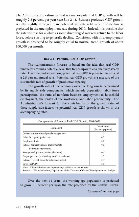
76 | Chapter 2
Box 2-1: Potential Real GDP Growth
The Administration forecast is based on the idea that real GDPfluctuates around a potential level that trends upward at a relatively steadyrate. Over the budget window, potential real GDP is projected to grow ata 2.5 percent annual rate. Potential real GDP growth is a measure of thesustainable rate of growth of productive capacity.
The growth rate of the economy over the long run is determinedby its supply side components, which include population, labor forceparticipation, the ratio of nonfarm business employment to householdemployment, the length of the workweek, and labor productivity. TheAdministration’s forecast for the contribution of the growth rates ofthese supply side factors to potential real GDP growth is shown in theaccompanying table.
Over the next 11 years, the working-age population is projectedto grow 1.0 percent per year, the rate projected by the Census Bureau.
The Administration estimates that normal or potential GDP growth will beroughly 2½ percent per year (see Box 2-1). Because projected GDP growthis only slightly stronger than potential growth, relatively little decline isprojected in the unemployment rate during 2010. Indeed, it is possible thatthe rate will rise for a while as some discouraged workers return to the laborforce, before starting to generally decline. Consistent with this, employmentgrowth is projected to be roughly equal to normal trend growth of about100,000 per month.
Continued on next page
Components of Potential Real GDP Growth, 2009-2020
Component Contribution(Percentage points)
Civilian noninstitutional population aged 16+ 1.0Labor force participation rate -0.3Employment rate 0.0Ratio of nonfarm business employment to -0.0
household employmentAverage weekly hours (nonfarm business) -0.1Output per hour (productivity, nonfarm business) 2.3Ratio of real GDP to nonfarm business output -0.4SUM: Real GDP 2.5Note: All contributions are in percentage points at an annual rate.Sources: CEA calculations; Department of the Treasury; Office of Management and Budget.
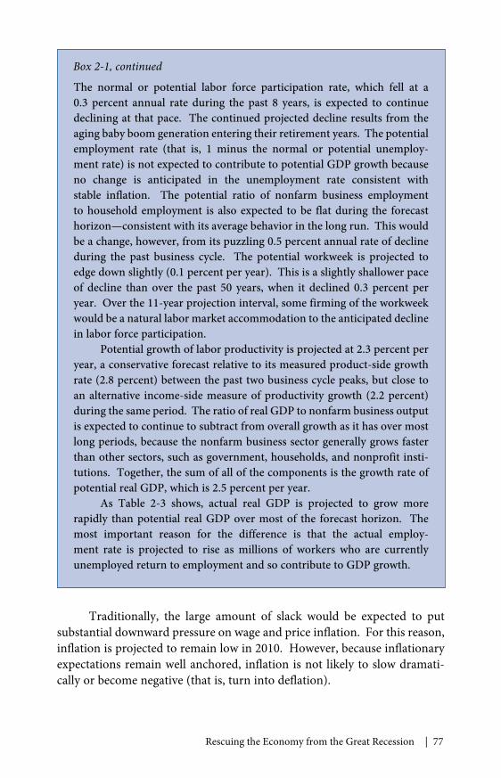
Rescuing the Economy from the Great Recession | 77
The normal or potential labor force participation rate, which fell at a0.3 percent annual rate during the past 8 years, is expected to continuedeclining at that pace. The continued projected decline results from theaging baby boom generation entering their retirement years. The potentialemployment rate (that is, 1 minus the normal or potential unemploy-ment rate) is not expected to contribute to potential GDP growth becauseno change is anticipated in the unemployment rate consistent withstable inflation. The potential ratio of nonfarm business employmentto household employment is also expected to be flat during the forecasthorizon—consistent with its average behavior in the long run. This wouldbe a change, however, from its puzzling 0.5 percent annual rate of declineduring the past business cycle. The potential workweek is projected toedge down slightly (0.1 percent per year). This is a slightly shallower paceof decline than over the past 50 years, when it declined 0.3 percent peryear. Over the 11-year projection interval, some firming of the workweekwould be a natural labor market accommodation to the anticipated declinein labor force participation.
Potential growth of labor productivity is projected at 2.3 percent peryear, a conservative forecast relative to its measured product-side growthrate (2.8 percent) between the past two business cycle peaks, but close toan alternative income-side measure of productivity growth (2.2 percent)during the same period. The ratio of real GDP to nonfarm business outputis expected to continue to subtract from overall growth as it has over mostlong periods, because the nonfarm business sector generally grows fasterthan other sectors, such as government, households, and nonprofit insti-tutions. Together, the sum of all of the components is the growth rate ofpotential real GDP, which is 2.5 percent per year.
As Table 2-3 shows, actual real GDP is projected to grow morerapidly than potential real GDP over most of the forecast horizon. Themost important reason for the difference is that the actual employ-ment rate is projected to rise as millions of workers who are currentlyunemployed return to employment and so contribute to GDP growth.
Traditionally, the large amount of slack would be expected to putsubstantial downward pressure on wage and price inflation. For this reason,inflation is projected to remain low in 2010. However, because inflationaryexpectations remain well anchored, inflation is not likely to slow dramati-cally or become negative (that is, turn into deflation).
Box 2-1, continued
78 | Chapter 2
In 2011, slightly higher GDP growth of approximately 4 percentis projected (again measured from fourth quarter to fourth quarter).Consistent with this, stronger employment growth and a more substantialdecline in the unemployment rate are expected in 2011. However, becauseGDP growth is still not projected to be as robust as that following someother deep recessions, continued large output gaps are anticipated. This willlimit the upward movement of the inflation rate toward a pace consistentwith the Federal Reserve’s long-term target inflation rate of about 2 percent.Moreover, employment growth is unlikely to be large enough to reduce theemployment shortfall dramatically in 2011.
Responsible Policies to Spur Job CreationThis large employment gap and the prospects that it is likely to recede
only slowly make a compelling case for additional measures to spur privatesector job creation. The Administration is therefore exploring a range ofpossibilities and working with Congress to pass measures into law.
Several principles are guiding this process. First, at a time whenthe budget deficit is large and the country faces significant long-run fiscalchallenges, measures must be cost-effective. Second, given that the employ-ment consequences of the recession have been severe, measures must focusparticularly on job creation. And third, measures must be tailored to thestate of the economy: the policies that are appropriate when an economy iscontracting rapidly may not be the same as those that are appropriate for aneconomy that is growing again but operating below capacity.
Guided by these principles, the Administration has identified three keypriorities. One is a multifaceted program to jump-start job creation by smallbusinesses, which are critical to growth and have been particularly harmedby the recession. Among the possible policies in this area are investmentincentives, tax incentives for hiring, and additional steps to increase the avail-ability of loans backed by the Small Business Administration. These policiesmay be particularly effective at a time when the economy is growing—so thatthe question for many firms is not whether to hire but when—and at a timewhen credit availability remains an important constraint.
Initiatives to encourage energy efficiency and clean energy are anotherpriority. One proposal involves incentives for homeowners to retrofittheir homes for energy efficiency. Because in many cases the effect of suchincentives would be to lead homeowners to make cost-saving investmentsearlier than they otherwise would have, they might have an especially largeimpact. In addition, the employment effects would be concentrated inconstruction, an area that has been particularly hard-hit by the recession.
Rescuing the Economy from the Great Recession | 79
The Administration has also supported extending tax credits through theDepartment of Energy that promote the manufacture of advanced energyproducts and providing incentives to increase the energy efficiency of publicand nonprofit buildings.
A third priority is infrastructure investment. The experience of theRecovery Act suggests that spending on infrastructure is an effective way toput people back to work while creating lasting investments that raise futureproductivity. For this reason, the Administration is supporting an addi-tional investment of up to $50 billion in roads, bridges, airports, transit, rail,and water projects. Funneling some of these funds through programs suchas the Transportation Investment Generating Economic Recovery (TIGER)program at the Department of Transportation, which is a competitive grantprogram, could offer a way to ensure that the projects with the highestreturns receive top priority.
Finally, it is critical to maintain our support for the individuals andfamilies most affected by the recession by extending the emergency fundingfor such programs as unemployment insurance and health insurance subsi-dies for the unemployed. This support not only cushions the worst effects ofthe downturn, but also boosts spending and so spurs job creation. Similarly,it is important to maintain support for state and local governments. Thebudgets of these governments remain under severe strain, and many arecutting back in anticipation of fiscal year 2011 deficits. Additional fiscalsupport could therefore have a rapid impact on spending, and would do soby maintaining crucial services and preventing harmful tax increases.
Conclusion
The recession that began at the end of 2007 became the “GreatRecession” following the financial crisis in the fall of 2008. In the wake ofthe collapse of Lehman Brothers in September, American families faceddevastating job losses, high unemployment, scarce credit, and lost wealth.Late 2008 and 2009 will be remembered as a time of great trial for Americanworkers, businesses, and families.
But 2009 should also be remembered as a year when even more tragiclosses and dislocation did not occur. As terrible as this recession has been,a second Great Depression would have been far worse. Had policymakersnot responded as aggressively as they did to shore up the financial system,maintain demand, and provide relief to those directly harmed by thedownturn, the outcome could have been much more dire.
As 2010 begins, there are strong signs that the American economy isstarting to recover. Housing and financial markets appear to have stabilized

80 | Chapter 2
and real GDP is growing again. The labor market also appears to be healing,showing the expected early pattern of response to output expansion.
With millions of Americans still unemployed, much work remains torestore the American economy to health. It will take a prolonged and robustGDP expansion to eliminate the large jobs deficit that has opened up overthe course of the recession. Only when the unemployment rate has returnedto normal levels and families are once again secure in their jobs, homes, andsavings will this terrible recession truly be over.