16

Chapter 2: Probability

The aim of this chapter is to revise the basic rules of probability. By the endof this chapter, you should be comfortable with:

• conditional probability, and what you can and can’t do with conditional

expressions;

• the Partition Theorem and Bayes’ Theorem;

• First-Step Analysis for finding the probability that a process reaches somestate, by conditioning on the outcome of the first step;

• calculating probabilities for continuous and discrete random variables.

2.1 Sample spaces and events

Definition: A sample space, Ω, is a set of possible outcomes of a randomexperiment.

Definition: An event, A, is a subset of the sample space.

This means that event A is simply a collection of outcomes.

Example:

Random experiment: Pick a person in this class at random.

Sample space: Ω = all people in classEvent A: A = all males in class.

Definition: Event A occurs if the outcome of the random experiment is a memberof the setA.

In the example above, event A occurs if the person we pick is male.

17

2.2 Probability Reference List

The following properties hold for all events A, B.

• P(∅) = 0.

• 0 ≤ P(A) ≤ 1.

• Complement: P(A) = 1− P(A).

• Probability of a union: P(A ∪B) = P(A) + P(B)− P(A ∩ B).

For three events A, B, C:

P(A∪B∪C) = P(A)+P(B)+P(C)−P(A∩B)−P(A∩C)−P(B∩C)+P(A∩B∩C) .

If A and B are mutually exclusive, then P(A ∪B) = P(A) + P(B).

• Conditional probability: P(A |B) =P(A ∩ B)

P(B).

• Multiplication rule: P(A ∩B) = P(A |B)P(B) = P(B |A)P(A).

• The Partition Theorem: if B1, B2, . . . , Bm form a partition of Ω, then

P(A) =m∑

i=1

P(A ∩Bi) =m∑

i=1

P(A |Bi)P(Bi) for any event A.

As a special case, B and B partition Ω, so:

P(A) = P(A ∩ B) + P(A ∩B)

= P(A |B)P(B) + P(A |B)P(B) for any A, B.

• Bayes’ Theorem: P(B |A) =P(A |B)P(B)

P(A).

More generally, if B1, B2, . . . , Bm form a partition of Ω, then

P(Bj |A) =P(A |Bj)P(Bj)

∑mi=1

P(A |Bi)P(Bi)for any j.

• Chains of events: for any events A1, A2, . . . , An,

P(A1∩A2∩ . . .∩An) = P(A1)P(A2 |A1)P(A3 |A2∩A1) . . .P(An |An−1∩ . . .∩A1).

2.3 Conditional Probability

Suppose we are working with sample spaceΩ = people in class. I want to find theproportion of people in the class who ski. What do I do?

Count up the number of people in the class who ski, and divide by the totalnumber of people in the class.

P(person skis) =number of skiers in class

total number of people in class.

Now suppose I want to find the proportion of females in the class who ski.

What do I do?

Count up the number of females in the class who ski, and divide bythe total number of females in the class.

P(female skis) =number of female skiers in class

total number of females in class.

By changing from asking about everyone to asking about females only, we have:

• restricted attention to the set of females only,

or: reduced the sample space from the set of everyone to the set of

females,

or: conditioned on the event females.

We could write the above as:

P(skis | female) =number of female skiers in class

total number of females in class.

Conditioning is like changing the sample space: we are now working ina new sample space of females in class.

19

In the above example, we could replace ‘skiing’ with any attribute B. We have:

P(skis) =# skiers in class

# class; P(skis | female) =

# female skiers in class

# females in class;

so:

P(B) =# B’s in class

total # people in class,

and:

P(B | female) =# female B’s in class

total # females in class

=# in class who are B and female

# in class who are female.

Likewise, we could replace ‘female’ with any attribute A:

P(B |A) =number in class who are B and A

number in class who are A.

This is how we get the definition of conditional probability:

P(B |A) =P(B and A)

P(A).=

P(B ∩ A)

P(A).

By conditioning on event A, we have changed the sample space to the set

of A’s only.

Definition: Let A and B be events on the same sample space: so A ⊆ Ω andB ⊆ Ω. The conditional probability of event B, given event A, is

P(B |A) =P(B ∩ A)

P(A).

20

Multiplication Rule: (Immediate from above). For any events A and B,

P(A ∩ B) = P(A |B)P(B) = P(B |A)P(A) = P(B ∩ A).

Conditioning as ‘changing the sample space’

The idea that “conditioning” = “changing the sample space” can be

very helpful in understanding how to manipulate conditional probabilities.

Any ‘unconditional’ probability can be written as a conditional probability:

P(B) = P(B |Ω).

Writing P(B) = P(B |Ω) just means that we are looking for the probability ofevent B, out of all possible outcomes in the set Ω.

In fact, the symbol P belongs to the set Ω: it has no meaning without Ω.

To remind ourselves of this, we can write

P = PΩ.

Then P(B) = P(B |Ω) = PΩ(B).

Similarly, P(B |A) means that we are looking for the probability of event B,out of all possible outcomes in the set A.

So A is just another sample space. Thus we can manipulate conditional

probabilities P( · |A) just like any other probabilities, as long as wealways stay inside the same sample space A.

The trick: Because we can think of A as just another sample space, let’s write

P( · |A) = PA( · )

Note: NOTstandard notation!

Then we can use PA just like P, as long as we remember to keep theA subscript on EVERY P that we write.

21

This helps us to make quite complex manipulations of conditional probabilitieswithout thinking too hard or making mistakes. There is only one rule you need

to learn to use this tool effectively:

PA(B |C) = P(B |C ∩ A) for any A, B, C.

(Proof: Exercise).

The rules: P( · |A) = PA( · )

PA(B |C) = P(B |C ∩ A) for any A, B, C.

Examples:

1. Probability of a union. In general,

P(B ∪ C) = P(B) + P(C)− P(B ∩ C).

So, PA(B ∪ C) = PA(B) + PA(C)− PA(B ∩ C).

Thus, P(B ∪ C |A) = P(B |A) + P(C |A)− P(B ∩ C |A).

2. Which of the following is equal to P(B ∩ C |A)?

(a) P(B |C ∩ A). (c) P(B |C ∩ A)P(C |A).

(b)P(B |C)

P(A). (d) P(B |C)P(C |A).

Solution:

P(B ∩ C |A) = PA(B ∩ C)

= PA(B |C)PA(C)

= P(B |C ∩ A)P(C |A).

Thus the correct answer is (c).

22

3. Which of the following is true?

(a) P(B |A) = 1− P(B |A). (b) P(B |A) = P(B)− P(B |A).

Solution:

P(B |A) = PA(B) = 1− PA(B) = 1− P(B |A).

Thus the correct answer is (a).

4. Which of the following is true?

(a) P(B ∩ A) = P(A)− P(B ∩ A). (b) P(B ∩ A) = P(B)− P(B ∩ A).

Solution:

P(B ∩ A) = P(B |A)P(A) = PA(B)P(A)

=(

1− PA(B))

P(A)

= P(A)− P(B |A)P(A)

= P(A)− P(B ∩ A).

Thus the correct answer is (a).

5. True or false: P(B |A) = 1− P(B |A) ?

Answer: False. P(B |A) = PA(B). Once we have PA, we are stuck with

it! There is no easy way of converting from PA to P A: or anythingelse. Probabilities in one sample space (PA) cannot tell us anything

about probabilities in a different sample space (P A).

Exercise: if we wish to express P(B |A) in terms of only B and A, show that

P(B |A) =P(B)− P(B |A)P(A)

1− P(A). Note that this does not simplify nicely!

23

2.4 The Partition Theorem (Law of Total Probability)

Definition: Events A and B are mutually exclusive, or disjoint, if A ∩B = ∅.

This means events A and B cannot happen together. If A happens, it excludes

B from happening, and vice-versa.

If A and B are mutually exclusive, P(A ∪B) = P(A) + P(B).For all other A and B, P(A ∪B) = P(A) + P(B)− P(A ∩B).

Definition: Any number of events B1, B2, . . . , Bk are mutually exclusive if every

pair of the events is mutually exclusive: ie. Bi ∩Bj = ∅ for all i, j with i 6= j.

Definition: A partition of Ω is a collection of mutually exclusive eventswhose union is Ω.

That is, sets B1, B2, . . . , Bk form a partition of Ω if

Bi ∩ Bj = ∅ for all i, j with i 6= j ,

and

k⋃

i=1

Bi = B1 ∪B2 ∪ . . . ∪Bk = Ω.

B1, . . . , Bk form a partition of Ω if they have no overlapand collectively cover all possible outcomes.

24

Examples:

Partitioning an event A

Any set A can be partitioned: it doesn’t have to be Ω.

In particular, if B1, . . . , Bk form a partition of Ω, then (A ∩ B1), . . . , (A ∩ Bk)form a partition of A.

Theorem 2.4: The Partition Theorem (Law of Total Probability)

Let B1, . . . , Bm form a partition of Ω. Then for any event A,

P(A) =m∑

i=1

P(A ∩ Bi) =m∑

i=1

P(A |Bi)P(Bi)

Both formulations of the Partition Theorem are very widely used, but especially

the conditional formulation∑m

i=1P(A |Bi)P(Bi).

25

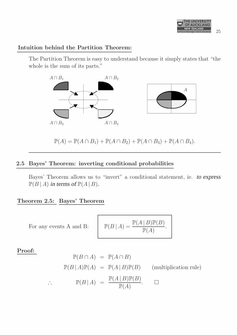
Intuition behind the Partition Theorem:

The Partition Theorem is easy to understand because it simply states that “thewhole is the sum of its parts.”

A

A ∩B1 A ∩B2

A ∩B3 A ∩B4

P(A) = P(A ∩ B1) + P(A ∩B2) + P(A ∩ B3) + P(A ∩B4).

2.5 Bayes’ Theorem: inverting conditional probabilities

Bayes’ Theorem allows us to “invert” a conditional statement, ie. to expressP(B |A) in terms ofP(A |B).

Theorem 2.5: Bayes’ Theorem

For any events A and B: P(B |A) =P(A |B)P(B)

P(A).

Proof:P(B ∩ A) = P(A ∩B)

P(B |A)P(A) = P(A |B)P(B) (multiplication rule)

∴ P(B |A) =P(A |B)P(B)

P(A).

26

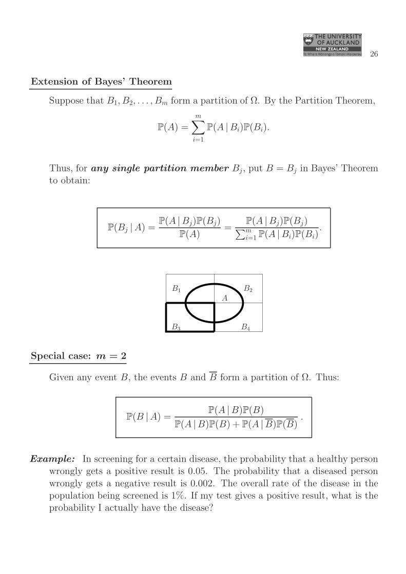
Extension of Bayes’ Theorem

Suppose that B1, B2, . . . , Bm form a partition of Ω. By the Partition Theorem,

P(A) =m∑

i=1

P(A |Bi)P(Bi).

Thus, for any single partition member Bj, put B = Bj in Bayes’ Theoremto obtain:

P(Bj |A) =P(A |Bj)P(Bj)

P(A)=

P(A |Bj)P(Bj)∑m

i=1P(A |Bi)P(Bi)

.

AB1 B2

B3 B4

Special case: m = 2

Given any event B, the events B and B form a partition of Ω. Thus:

P(B |A) =P(A |B)P(B)

P(A |B)P(B) + P(A |B)P(B).

Example: In screening for a certain disease, the probability that a healthy personwrongly gets a positive result is 0.05. The probability that a diseased person

wrongly gets a negative result is 0.002. The overall rate of the disease in thepopulation being screened is 1%. If my test gives a positive result, what is theprobability I actually have the disease?

27

1. Define events:

D = have disease D = do not have the disease

P = positive test N = P = negative test

2. Information given:

False positive rate is 0.05 ⇒ P(P |D) = 0.05

False negative rate is 0.002 ⇒ P(N |D) = 0.002

Disease rate is 1% ⇒ P(D) = 0.01.

3. Looking for P(D |P ):

We have P(D |P ) =P(P |D)P(D)

P(P ).

Now P(P |D) = 1− P(P |D)

= 1− P(N |D)

= 1− 0.002

= 0.998.

Also P(P ) = P(P |D)P(D) + P(P |D)P(D)

= 0.998× 0.01 + 0.05× (1− 0.01)

= 0.05948.

Thus

P(D |P ) =0.998× 0.01

0.05948= 0.168.

Given a positive test, my chance of having the disease is only 16.8%.

28

2.6 First-Step Analysis for calculating probabilities in a process

In a stochastic process, what happens at the next step depends upon the cur-rent state of the process. We often wish to know the probability of eventually

reaching some particular state, given our current position.

Throughout this course, we will tackle this sort of problem using a techniquecalled First-Step Analysis.

The idea is to consider all possible first steps away from the current state. Wederive a system of equations that specify the probability of the eventual outcome

given each of the possible first steps. We then try to solve these equations forthe probability of interest.

First-Step Analysis depends upon conditional probability and thePartition

Theorem. Let S1, . . . , Sk be the k possible first steps we can take away from ourcurrent state. We wish to find the probability that event E happens eventually.First-Step Analysis calculates P(E) as follows:

P(E) = P(E|S1)P(S1) + . . .+ P(E|Sk)P(Sk).

Here, P(S1), . . . ,P(Sk) give the probabilities of taking the different first steps

1, 2, . . . , k.

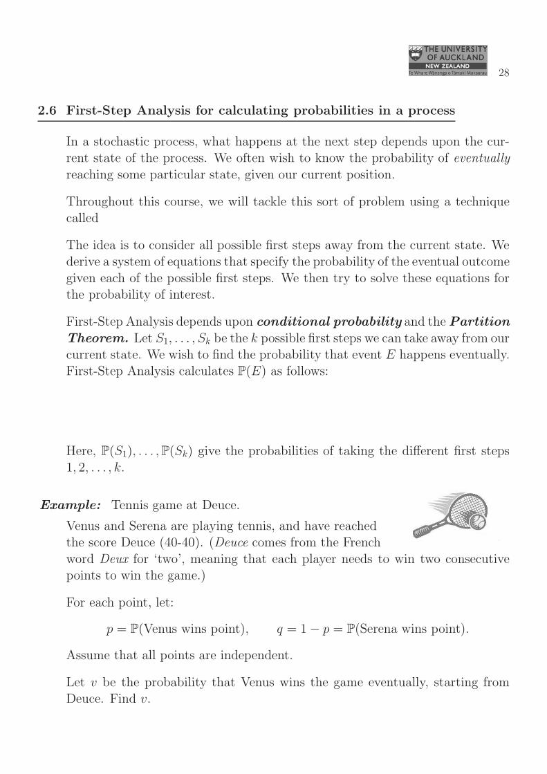
Example: Tennis game at Deuce.

Venus and Serena are playing tennis, and have reachedthe score Deuce (40-40). (Deuce comes from the French

word Deux for ‘two’, meaning that each player needs to win two consecutivepoints to win the game.)

For each point, let:

p = P(Venus wins point), q = 1− p = P(Serena wins point).

Assume that all points are independent.

Let v be the probability that Venus wins the game eventually, starting fromDeuce. Find v.

29

VENUSWINS (W)

VENUSAHEAD (A)

VENUSBEHIND (B)

p

q

p p

qq

VENUSLOSES (L)

DEUCE (D)

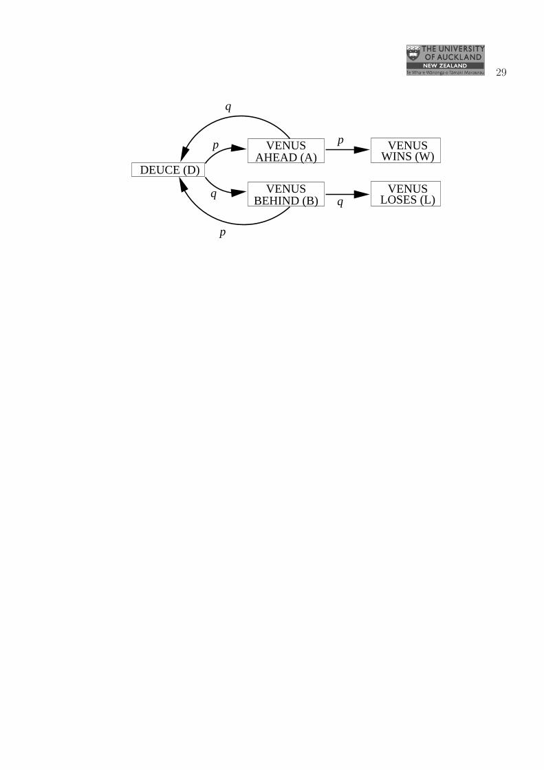
Use First-step analysis. The possible steps starting from Deuce are:

1. Venus wins the next point (probability p): move to state A;

2. Venus loses the next point (probability q): move to state B.

Let V be the event that Venus wins EVENTUALLY starting fromDeuce, so v = P(V |D). Starting from Deuce (D), the possible steps

are to states A and B. So:v = P(Venus wins |D) = P(V |D)

= PD(V )

= PD(V |A)PD(A) + PD(V |B)PD(B)

= P(V |A)p+ P(V |B)q. (⋆)

Now we need to find P(V |A), and P(V |B), again using First-stepanalysis:

P(V |A) = P(V |W )p+ P(V |D)q

= 1× p+ v × q

= p + qv. (a)

Similarly,

P(V |B) = P(V |L)q + P(V |D)p

= 0× q + v × p

= pv. (b)

30

Substituting (a) and (b) into (⋆),

v = (p+ qv)p+ (pv)q

v = p2 + 2pqv

v(1− 2pq) = p2

v =p2

1− 2pq.

Note: Because p+ q = 1, we have:

1 = (p+ q)2 = p2 + q2 + 2pq.

So the final probability that Venus wins the game is:

v =p2

1− 2pq=

p2

p2 + q2.

Note how this result makes intuitive sense. For the game to finish from Deuce,either Venus has to win two points in a row (probability p2), or Serena does

(probability q2). The ratio p2/(p2+ q2) describes Venus’s ‘share’ of the winningprobability.

First-step analysis as the Partition Theorem:

Our approach to finding v = P(Venus wins) can be summarized as:

P(Venus wins) = v =∑

first steps

P(V |first step)P(first step) .

First-step analysis is just the Partition Theorem:

The sample space is Ω = all possible routes from Deuce to the end .

An example of a sample point is: D → A → D → B → D → B → L.

Another example is: D → B → D → A → W.

The partition of the sample space that we use in first-step analysis is:

R1 = all possible routes from Deuce to the end that start with D → A

R2 = all possible routes from Deuce to the end that start with D → B

31

Then first-step analysis simply states:

P(V ) = P(V |R1)P(R1) + P(V |R2)P(R2)

= PD(V |A)PD(A) + PD(V |B)PD(B).

Notation for quick solutions of first-step analysis problems

Defining a helpful notation is central to modelling with stochastic processes.

Setting up well-defined notation helps you to solve problems quickly and easily.Defining your notation is one of the most important steps in modelling, becauseit provides the conversion from words (which is how your problem starts) to

mathematics (which is how your problem is solved).

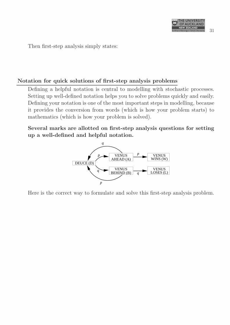
Several marks are allotted on first-step analysis questions for settingup a well-defined and helpful notation.

VENUSWINS (W)

VENUSAHEAD (A)

VENUSBEHIND (B)

p

q

p p

qq

VENUSLOSES (L)

DEUCE (D)

Here is the correct way to formulate and solve this first-step analysis problem.

Need the probability that Venus wins eventually, starting from Deuce.1. Define notation: let

vD = P(Venus wins eventually | start at state D)

vA = P(Venus wins eventually | start at state A)

vB = P(Venus wins eventually | start at state B)

2. First-step analysis:vD = pvA + qvB (a)

vA = p× 1 + qvD (b)

vB = pvD + q × 0 (c)

32

3. Substitute (b) and (c) in (a):

⇒ vD = p(p+ qvD) + q(pvD)

vD(1− pq − pq) = p2

∴ vD =p2

1− 2pq

as before.

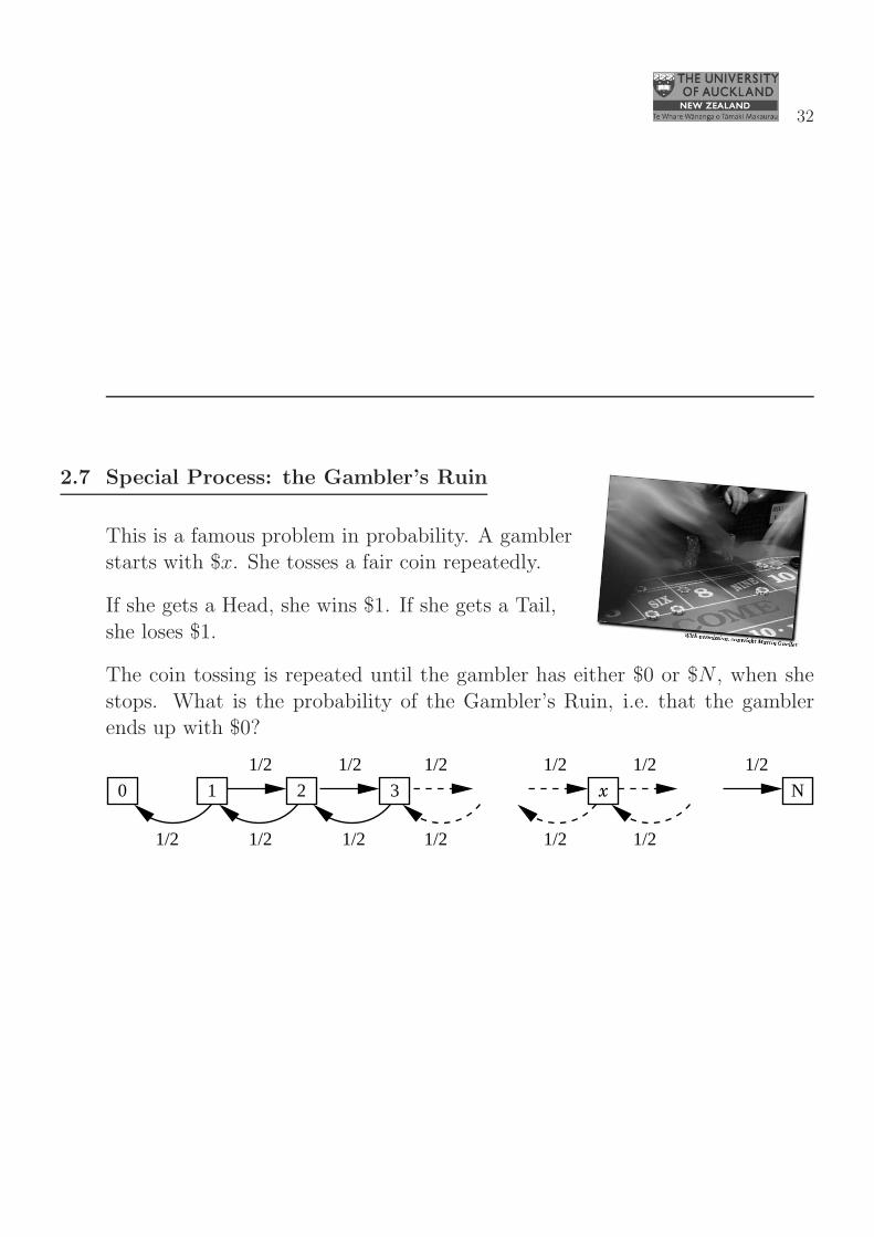
2.7 Special Process: the Gambler’s Ruin

This is a famous problem in probability. A gamblerstarts with $x. She tosses a fair coin repeatedly.

If she gets a Head, she wins $1. If she gets a Tail,

she loses $1.

The coin tossing is repeated until the gambler has either $0 or $N , when she

stops. What is the probability of the Gambler’s Ruin, i.e. that the gamblerends up with $0?

1/2

1/2

1/2

1/2

1/2

1/2

0 1 2 3

1/2 1/2

1/2 1/21/2

N

1/2

x

Wish to find

P(ends with $0 | starts with $x) .

Define event

R = eventual Ruin = ends with $0 .

We wish to find P(R | starts with $x).

Define notation:

px = P(R | currently has $x) for x = 0, 1, . . . , N.

33

Information given:p0 = P(R | currently has $0) = 1,

pN = P(R | currently has $N) = 0.

First-step analysis:

px = P(R |has $x)

= 1

2P

(

R |has $(x+ 1))

+ 1

2P

(

R |has $(x− 1))

= 1

2px+1 +

1

2px−1 (⋆)

True for x = 1, 2, . . . , N − 1, with boundary conditions p0 = 1, pN = 0.

Solution of difference equation (⋆):

px = 1

2px+1 + 1

2px−1 for x = 1, 2, . . . , N − 1 ;

p0 = 1 (⋆)

pN = 0.

We usually solve equations like this using the theory of 2nd-order differenceequations. For this special case we will also verify the answer by two other

methods.

1. Theory of linear 2nd order difference equations

Theory tells us that the general solution of(⋆) is px = A+Bx for some constantsA, B and forx = 0, 1, . . . , N . Our job is to findA andB using the boundaryconditions:

px = A+ Bx for constants A and B and for x = 0, 1, . . . , N.

So

p0 = A+B × 0 = 1 ⇒ A = 1 ;

pN = A+B ×N = 1 + BN = 0 ⇒ B = −1

N.

34

So our solution is: px = A+ B x = 1−x

Nfor x = 0, 1, . . . , N.

For Stats 325, you will be told the general solution of the 2nd-order difference

equation and expected to solve it using the boundary conditions.

For Stats 721, we will study the theory of 2nd-order difference equations. Youwill be able to derive the general solution for yourself before solving it.

Question: What is the probability that the gambler wins (ends with $N),

starting with $x?

P

(

ends with $N)

= 1−P

(

ends with $0)

= 1−px =x

Nfor x = 0, 1, . . . , N.

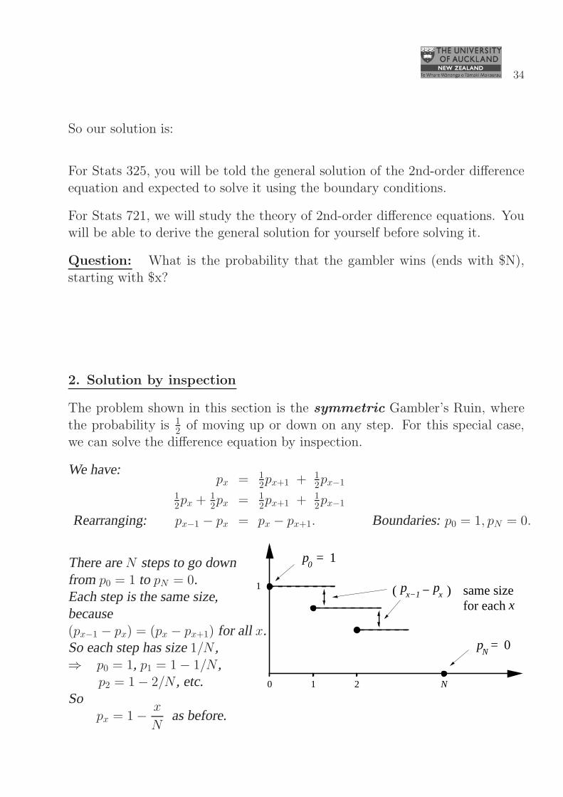
2. Solution by inspection

The problem shown in this section is the symmetric Gambler’s Ruin, where

the probability is 1

2of moving up or down on any step. For this special case,

we can solve the difference equation by inspection.

We have:px = 1

2px+1 + 1

2px−1

1

2px +

1

2px = 1

2px+1 + 1

2px−1

Rearranging: px−1 − px = px − px+1. Boundaries:p0 = 1, pN = 0.

1 2 N

1 − p( ) same sizefor each

0p = N

0

px−1 x

1p = 0

x

There areN steps to go downfrom p0 = 1 to pN = 0.Each step is the same size,because(px−1 − px) = (px − px+1) for all x.So each step has size1/N ,⇒ p0 = 1, p1 = 1− 1/N ,

p2 = 1− 2/N , etc.So

px = 1−x

Nas before.

35

3. Solution by repeated substitution.

In principle, all systems could be solved by this method, but it is usually tootedious to apply in practice.

Rearrange(⋆) to give:

px+1 = 2px − px−1

⇒ (x = 1) p2 = 2p1 − 1 (recallp0 = 1)

(x = 2) p3 = 2p2 − p1 = 2(2p1 − 1)− p1 = 3p1 − 2

(x = 3) p4 = 2p3 − p2 = 2(3p1 − 2)− (2p1 − 1) = 4p1 − 3 etc...

giving px = xp1 − (x− 1) in general, (⋆⋆)

likewise pN = Np1 − (N − 1) at endpoint.

Boundary condition: pN = 0 ⇒ Np1 − (N − 1) = 0 ⇒ p1 = 1− 1/N.

Substitute in(⋆⋆):

px = xp1 − (x− 1)

= x(

1− 1

N

)

− (x− 1)

= x− xN− x+ 1

px = 1− xN

as before.

2.8 Independence

Definition: Events A and B are statistically independent if and only if

P(A ∩ B) = P(A)P(B).

This implies that A and B are statistically independent if and only if

P(A |B) = P(A).

Note: If events are physically independent, they will also be statistically indept.

36

For interest: more than two events

Definition: For more than two events, A1, A2, . . . , An, we say that A1, A2, . . . , An

are mutually independent if

P

(

⋂

i∈J

Ai

)

=∏

i∈J

P(Ai) for ALL finite subsetsJ ⊆ 1, 2, . . . , n.

Example: events A1, A2, A3, A4 are mutually independent if

i) P(Ai ∩ Aj) = P(Ai)P(Aj) for all i, j with i 6= j; AND

ii) P(Ai∩Aj∩Ak) = P(Ai)P(Aj)P(Ak) for all i, j, k that are all different; AND

iii) P(A1 ∩ A2 ∩ A3 ∩ A4) = P(A1)P(A2)P(A3)P(A4).

Note: For mutual independence, it is not enough to check that P(Ai ∩ Aj) =

P(Ai)P(Aj) for all i 6= j. Pairwise independence does not imply mutual inde-pendence.

2.9 The Continuity Theorem

The Continuity Theorem states that probability is a continuous set function:

Theorem 2.9: The Continuity Theorem

a) Let A1, A2, . . . be an increasing sequence of events: i.e.

A1 ⊆ A2 ⊆ . . . ⊆ An ⊆ An+1 ⊆ . . . .

ThenP

(

limn→∞

An

)

= limn→∞

P(An).

Note: because A1 ⊆ A2 ⊆ . . ., we have: limn→∞

An =∞⋃

n=1

An.

37

b) Let B1, B2, . . . be a decreasing sequence of events: i.e.

B1 ⊇ B2 ⊇ . . . ⊇ Bn ⊇ Bn+1 ⊇ . . . .

ThenP

(

limn→∞

Bn

)

= limn→∞

P(Bn).

Note: because B1 ⊇ B2 ⊇ . . ., we have: limn→∞

Bn =

∞⋂

n=1

Bn.

Proof (a) only: for (b), take complements and use (a).

Define C1 = A1, and Ci = Ai\Ai−1 for i = 2, 3, . . .. Then C1, C2, . . . are mutuallyexclusive, and

⋃ni=1

Ci =⋃n

i=1Ai , and likewise,

⋃∞i=1

Ci =⋃∞

i=1Ai.

Thus

P( limn→∞

An) = P

(

∞⋃

i=1

Ai

)

= P

(

∞⋃

i=1

Ci

)

=∞∑

i=1

P(Ci) (Ci mutually exclusive)

= limn→∞

n∑

i=1

P(Ci)

= limn→∞

P

(

n⋃

i=1

Ci

)

= limn→∞

P

(

n⋃

i=1

Ai

)

= limn→∞

P(An).

38

2.10 Random Variables

Definition: A random variable, X, is defined as a function from the sample spaceto the real numbers:X : Ω → R.

A random variable therefore assigns a real number to every possible outcome ofa random experiment.

A random variable is essentially a rule or mechanism for generating random realnumbers.

The Distribution Function

Definition: The cumulative distribution function of a random variable X isgiven by

FX(x) = P(X ≤ x)

FX(x) is often referred to as simply the distribution function.

Properties of the distribution function

1) FX(−∞) = P(X ≤ −∞) = 0.

FX(+∞) = P(X ≤ ∞) = 1.

2) FX(x) is a non-decreasing function of x:if x1 < x2, thenFX(x1) ≤ FX(x2).

3) If b > a, then P(a < X ≤ b) = FX(b)− FX(a).

4) FX is right-continuous: i.e. limh↓0 FX(x+ h) = FX(x).

39

2.11 Continuous Random Variables

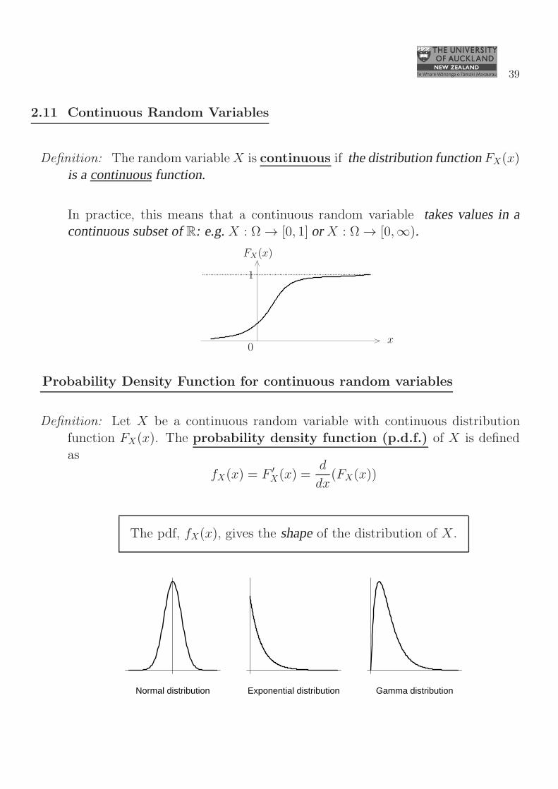
Definition: The random variableX is continuous if the distribution functionFX(x)

is a continuousfunction.

In practice, this means that a continuous random variable takes values in acontinuous subset ofR: e.g.X : Ω → [0, 1] or X : Ω → [0,∞).

x

FX(x)

0

1

Probability Density Function for continuous random variables

Definition: Let X be a continuous random variable with continuous distribution

function FX(x). The probability density function (p.d.f.) of X is definedas

fX(x) = F ′X(x) =

d

dx(FX(x))

The pdf, fX(x), gives the shapeof the distribution of X.

Normal distribution Exponential distribution Gamma distribution

40

By the Fundamental Theorem of Calculus, the distribution function FX(x) canbe written in terms of the probability density function, fX(x), as follows:

FX(x) =∫ x

−∞ fX(u) du

Endpoints of intervals

For continuous random variables, every point x has P(X = x) = 0. Thismeans that the endpoints of intervals are not important for continuous random

variables.

Thus, P(a ≤ X ≤ b) = P(a < X ≤ b) = P(a ≤ X < b) = P(a < X < b).

This is only true for continuous random variables.

Calculating probabilities for continuous random variables

To calculate P(a ≤ X ≤ b), use either

P(a ≤ X ≤ b) = FX(b)− FX(a)

or

P(a ≤ X ≤ b) =

∫ b

a

fX(x) dx

Example: Let X be a continuous random variable with p.d.f.

fX(x) =

2x−2 for 1 < x < 2,

0 otherwise.

(a) Find the cumulative distribution function, FX(x).

(b) Find P (X ≤ 1.5).

41

a) FX(x) =

∫ x

−∞

fX(u) du =

∫ x

1

2u−2 du =

[

2u−1

−1

]x

1

= 2−2

xfor 1 < x < 2.

ThusFX(x) =

0 for x ≤ 1,

2− 2

xfor 1 < x < 2,

1 for x ≥ 2.

b) P(X ≤ 1.5) = FX(1.5) = 2−2

1.5=

2

3.

2.12 Discrete Random Variables

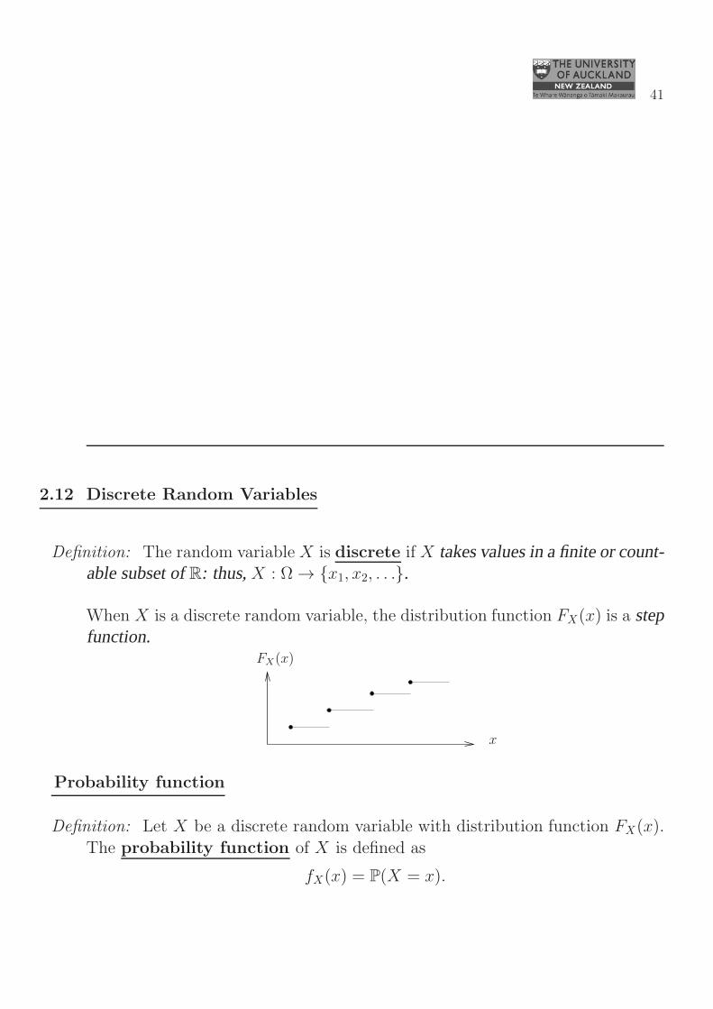
Definition: The random variable X is discrete if X takes values in a finite orcount-able subset of R: thus, X : Ω → x1, x2, . . ..

When X is a discrete random variable, the distribution function FX(x) is a stepfunction.

x

FX(x)

Probability function

Definition: Let X be a discrete random variable with distribution function FX(x).

The probability function of X is defined as

fX(x) = P(X = x).

42

Endpoints of intervals

For discrete random variables, individual points can have P(X = x) > 0.

This means that the endpoints of intervals ARE important for discrete randomvariables.

For example, if X takes values 0, 1, 2, . . ., and a, b are integers with b > a, then

P(a ≤ X ≤ b) = P(a−1 < X ≤ b) = P(a ≤ X < b+1) = P(a−1 < X < b+1).

Calculating probabilities for discrete random variables

To calculate P(X ∈ A) for any countable set A, use

P(X ∈ A) =∑

x∈A

P(X = x).

Partition Theorem for probabilities of discrete random variables

Recall the Partition Theorem: for any event A, and for events B1, B2, . . . thatform a partition of Ω,

P(A) =∑

y

P(A |By)P(By).

We can use the Partition Theorem to find probabilities for random variables.Let X and Y be discrete random variables.

• Define event A as A = X = x.

• Define event By as By = Y = y for y = 0, 1, 2, . . . (or whatever

values Y takes).

• Then, by the Partition Theorem,

P(X = x) =∑

y

P(X = x |Y = y)P(Y = y).

43

2.13 Independent Random Variables

Random variables X and Y are independent if they have no effect on eachother. This means that the probability that they both take specified values

simultaneously is the product of the individual probabilities.

Definition: Let X and Y be random variables. The joint distribution function

of X and Y is given by

FX,Y (x, y) = P(X ≤ x and Y ≤ y) = P(X ≤ x, Y ≤ y).

Definition: Let X and Y be any random variables (continuous or discrete). X andY are independent if

FX,Y (x, y) = FX(x)FY (y) for ALL x, y ∈ R.

If X and Y are discrete, they are independent if and only if their joint prob-ability function is the product of their individual probability functions:

Discrete X, Y are indept ⇐⇒ P(X = x AND Y = y) = P(X = x)P(Y = y)

for ALL x, y⇐⇒ fX,Y (x, y) = fX(x)fY (y) for ALL x, y.