Chapter 2 Phase Plane Analysis - WordPress.com · Chapter 2 Phase Plane Analysis Phase plane...

Chapter 2Phase Plane Analysis

Phase plane analysis is a graphical method for studying second-order systems, whichwas introduced well before the turn of the century by mathematicians such as HenriPoincare. The basic idea of the method is to generate, in the state space of a second-order dynamic system (a two-dimensional plane called the phase plane), motiontrajectories corresponding to various initial conditions, and then to examine thequalitative features of the trajectories. In such a way, information concerning stabilityand other motion patterns of the system can be obtained. In this chapter, our objectiveis to gain familiarity with nonlinear systems through this simple graphical method.

Phase plane analysis has a number of useful properties. First, as a graphicalmethod, it allows us to visualize what goes on in a nonlinear system starting fromvarious initial conditions, without having to solve the nonlinear equations analytically.Second, it is not restricted to small or smooth nonlinearities, but applies equally wellto strong nonlinearities and to "hard" nonlinearities. Finally, some practical controlsystems can indeed be adequately approximated as second-order systems, and thephase plane method can be used easily for their analysis. Conversely, of course, thefundamental disadvantage of the method is that it is restricted to second-order (or first-order) systems, because the graphical study of higher-order systems iscomputationally and geometrically complex.

17

18 Phase Plane Analysis Chap. 2

2.1 Concepts of Phase Plane Analysis

2.1.1 Phase Portraits

The phase plane method is concerned with the graphical study of second-orderautonomous systems described by

x2=f2(Xl,x2) (2.1b)

where jq and x2 are the states of the system, and/ , and/ 2 are nonlinear functions ofthe states. Geometrically, the state space of this system is a plane having x, and x2 ascoordinates. We will call this plane the phase plane.

Given a set of initial conditions x(0) = x0, Equation (2.1) defines a solutionx(0- With time / varied from zero to infinity, the solution x(t) can be representedgeometrically as a curve in the phase plane. Such a curve is called a phase planetrajectory. A family of phase plane trajectories corresponding to various initialconditions is called a phase portrait of a system.

To illustrate the concept of phase portrait, let us consider the following simplesystem.

Example 2.1: Phase portrait of a mass-spring system

The governing equation of the mass-spring system in Figure 2.1 (a) is the familiar linear second-

order differential equation

x+x = Q (2.2)

Assume that the mass is initially at rest, at length xo . Then the solution of the equation is

x(l) = xo cos t

x(t) = — A'osin(

Eliminating time / from the above equations, we obtain the equation of the trajectories

This represents a circle in the phase plane. Corresponding to different initial conditions, circles of

different radii can be obtained. Plotting these circles on the phase plane, we obtain a phase

portrait for the mass-spring system (Figure 2.1 .b). U

Sect. 2.1 Concepts of Phase Plane Analysis 19

k= 1 m = l

(a) (b)

Figure 2.1 : A mass-spring system and its phase portrait

The power of the phase portrait lies in the fact that once the phase portrait of asystem is obtained, the nature of the system response corresponding to various initialconditions is directly displayed on the phase plane. In the above example, we easilysee that the system trajectories neither converge to the origin nor diverge to infinity.They simply circle around the origin, indicating the marginal nature of the system'sstability.

A major class of second-order systems can be described by differentialequations of the form

x +f(x, x) = 0

In state space form, this dynamics can be represented as

k\=x2

(2.3)

with A| = x and JT2 = -*• Most second-order systems in practice, such as mass-damper-spring systems in mechanics, or resistor-coil-capacitor systems in electricalengineering, can be represented in or transformed into this form. For these systems,the states are x and its derivative x. Traditionally, the phase plane method isdeveloped for the dynamics (2.3), and the phase plane is defined as the plane having xand x as coordinates. But it causes no difficulty to extend the method to more generaldynamics of the form (2.1), with the (xj , xj) plane as the phase plane, as we do in thischapter.


2.1.2 Singular Points

An important concept in phase plane analysis is that of a singular point. A singularpoint is an equilibrium point in the phase plane. Since an equilibrium point is definedas a point where the system states can stay forever, this implies that x = 0, and using

(2.1),

/ , (* , , JC2) = 0 /2(jr1,jr2) = 0 (2.4)

The values of the equilibrium states can be solved from (2.4).

For a linear system, there is usually only one singular point (although in somecases there can be a continuous set of singular points, as in the system x + x = 0, forwhich all points on the real axis are singular points). However, a nonlinear systemoften has more than one isolated singular point, as the following example shows.

Example 2.2: A nonlinear second-order system

Consider the system

x + 0.6 x + 3 x + x1 = 0

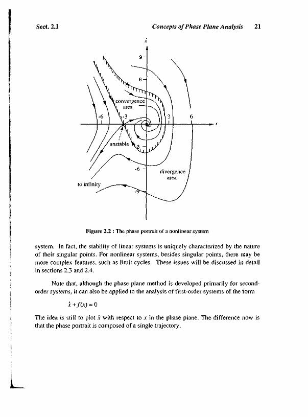
whose phase portrait is plotted in Figure 2.2. The system has two singular points, one at (0, 0)

and the other at (-3, 0). The motion patterns of the system trajectories in the vicinity of the two

singular points have different natures. The trajectories move towards the point x = 0 while

moving away from the point x = — 3. D

One may wonder why an equilibrium point of a second-order system is called asingular point. To answer this, let us examine the slope of the phase trajectories.From (2.1), the slope of the phase trajectory passing through a point (X|,x2) isdetermined by

2 J2\ ! V ( 2 5 )

dx\ f\(xx,x2)

With the functions / ] and f2 assumed to be single valued, there is usually a definitevalue for this slope at any given point in phase plane. This implies that the phasetrajectories will not intersect. At singular points, however, the value of the slope is0/0, i.e., the slope is indeterminate. Many trajectories may intersect at such points, asseen from Figure 2.2. This indeterminacy of the slope accounts for the adjective"singular".

Singular points are very important features in the phase plane. Examination ofthe singular points can reveal a great deal of information about the properties of a

Sect. 2.1 Concepts of Phase Plane Analysis 21

to infinity

Figure 2.2 : The phase portrait of a nonlinear system

system. In fact, the stability of linear systems is uniquely characterized by the natureof their singular points. For nonlinear systems, besides singular points, there may bemore complex features, such as limit cycles. These issues will be discussed in detailin sections 2.3 and 2.4.

Note that, although the phase plane method is developed primarily for second-order systems, it can also be applied to the analysis of first-order systems of the form

x +f(x) = 0

The idea is still to plot x with respect to x in the phase plane. The difference now isthat the phase portrait is composed of a single trajectory.

22 Phase Plane Analysis

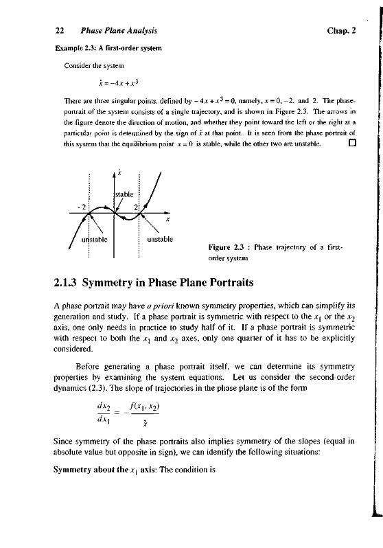
Example 2.3: A first-order system

Consider the system

Chap. 2

There are three singular points, defined by - 4x + x 3 = 0, namely, x = 0, - 2 , and 2. The phase-

portrait of the system consists of a single trajectory, and is shown in Figure 2.3. The arrows in

the figure denote the direction of motion, and whether they point toward the left or the right at a

particular point is determined by the sign of x at that point. It is seen from the phase portrait of

this system that the equilibrium point x = 0 is stable, while the other two are unstable. O

stable

unstableFigure 2.3 : Phase trajectory of a first-

order system

2.1.3 Symmetry in Phase Plane Portraits

A phase portrait may have a priori known symmetry properties, which can simplify itsgeneration and study. If a phase portrait is symmetric with respect to the X\ or the x2

axis, one only needs in practice to study half of it. If a phase portrait is symmetricwith respect to both the Xj and x2 axes, only one quarter of it has to be explicitlyconsidered.

Before generating a phase portrait itself, we can determine its symmetryproperties by examining the system equations. Let us consider the second-orderdynamics (2.3). The slope of trajectories in the phase plane is of the form

dx2 f{x\,x2)dx,1

Since symmetry of the phase portraits also implies symmetry of the slopes (equal inabsolute value but opposite in sign), we can identify the following situations:

Symmetry about the xi axis: The condition is

Sect. 2.2 Constructing Phase Portraits 23

f(xhx2) = f(xl,-x2)

This implies that the function / should be even in x2- The mass-spring system inExample 2.1 satisfies this condition. Its phase portrait is seen to be symmetric about

axis.

Symmetry about the x2 axis: Similarly,

f(x\,x2) = -f(-xl,x2)

implies symmetry with respect to the x2 axis. The mass-spring system also satisfiesthis condition.

Symmetry about the origin: When

f{x{,x2) = -f(-xh-x2)

the phase portrait of the system is symmetric about the origin.

2.2 Constructing Phase Portraits

Today, phase portraits are routinely computer-generated. In fact, it is largely theadvent of the computer in the early 1960's, and the associated ease of quicklygenerating phase portraits, which spurred many advances in the study of complexnonlinear dynamic behaviors such as chaos. However, of course (as e.g., in the case ofroot locus for linear systems), it is still practically useful to learn how to roughlysketch phase portraits or quickly verify the plausibility of computer outputs.

There are a number of methods for constructing phase plane trajectories forlinear or nonlinear systems, such as the so-called analytical method, the method ofisoclines, the delta method, Lienard's method, and Pell's method. We shall discusstwo of them in this section, namely, the analytical method and the method of isoclines.These methods are chosen primarily because of their relative simplicity. Theanalytical method involves the analytical solution of the differential equationsdescribing the systems. It is useful for some special nonlinear systems, particularlypiece-wise linear systems, whose phase portraits can be constructed by piecingtogether the phase portraits of the related linear systems. The method of isoclines is agraphical method which can conveniently be applied to construct phase portraits forsystems which cannot be solved analytically, which represent by far the most commoncase.


ANALYTICAL METHOD

There are two techniques for generating phase plane portraits analytically. Bothtechniques lead to a functional relation between the two phase variables Xj and x2 inthe form

g(xhx2,c) = 0 (2.6)

where the constant c represents the effects of initial conditions (and, possibly, ofexternal input signals). Plotting this relation in the phase plane for different initialconditions yields a phase portrait.

The first technique involves solving equations (2.1) forx[ and x2 as functions oftime t, i.e.,

and then eliminating time t from these equations, leading to a functional relation in theform of (2.6). This technique was already illustrated in Example 2.1.

The second technique, on the other hand, involves directly eliminating the timevariable, by noting that

and then solving this equation for a functional relation between Xj and x2. Let us usethis technique to solve the mass-spring equation again.

Example 2.4: Mass-spring system

By noting that x = (dx/dx)(dx/dt), we can rewrite (2.2) as

-v — + x = 0dx

Integration of this equation yields

i 2 + x 2 =xo2 •

One sees that the second technique is more straightforward in generating the equationsfor the phase plane trajectories.

Most nonlinear systems cannot be easily solved by either of the above twotechniques. However, for piece-wise linear systems, an important class of nonlinearsystems, this method can be conveniently used, as the following example shows.

L

Sect. 2.2

Example 2.5: A satellite control system

Constructing Phase Portraits 25

Figure 2.4 shows the control system for a simple satellite model. The satellite, depicted in Figure

2.5(a), is simply a rotational unit inertia controlled by a pair of thrusters, which can provide either

a positive constant torque U (positive firing) or a negative torque — U (negative firing). The

purpose of the control system is to maintain the satellite antenna at a zero angle by appropriately

firing the thrusters. The mathematical model of the satellite is

where w is the torque provided by the thrusters and 8 is the satellite angle.

Jets Satellite

ed = o U' —

-u

i u

1p

eip

Figure 2.4 : Satellite control system

Let us examine on the phase plane the behavior of the control system when the thrusters are

fired according to the control law

u(t) = / - U if 9 > 0w 1 u if e < o

(2.7)

which means that the thrusters push in the counterclockwise direction if G is positive, and vice

versa.

As the first step of the phase portrait generation, let us consider the phase portrait when the

thrusters provide a positive torque U. The dynamics of the system is

which implies that 6 dQ = U dQ. Therefore, the phase trajectories are a family of parabolas

defined by

where cf is a constant. The corresponding phase portrait of the system is shown in Figure 2.5(b).

When the thrusters provide a negative torque - U, the phase trajectories are similarly found

to be


u = -U

(a) (b) (c)

Figure 2.5 : Satellite control using on-off thrusters

with the corresponding phase portrait shown in Figure 2.5(c).

parabolictrajectories

u = +U

switching line

Figure 2.6 : Complete phase portrait of the control system

The complete phase portrait of the closed-loop control system can be obtained simply by

connecting the trajectories on the left half of the phase plane in 2.5(b) with those on the right half

of the phase plane in 2.5(c), as shown in Figure 2.6. The vertical axis represents a switching line,

because the control input and thus the phase trajectories are switched on that line. It is interesting

to see that, starting from a nonzero initial angle, the satellite will oscillate in periodic motions

i

Sect. 2.2 Constructing Phase Portraits 27

under the action of the jets. One concludes from this phase portrait that the system is marginally

stable, similarly to the mass-spring system in Example 2.1. Convergence of the system to the

zero angle can be obtained by adding rate feedback (Exercise 2.4). [3

THE METHOD OF ISOCLINES

The basic idea in this method is that of isoclines. Consider the dynamics in (2.1). At apoint (JCJ , x2) in the phase plane, the slope of the tangent to the trajectory can bedetermined by (2.5). An isocline is defined to be the locus of the points with a giventangent slope. An isocline with slope a is thus defined to be

dx2 _f2(xh x2) _

dxx fl(xl,x2)

This is to say that points on the curve

all have the same tangent slope a.

In the method of isoclines, the phase portrait of a system is generated in twosteps. In the first step, a field of directions of tangents to the trajectories is obtained. Inthe second step, phase plane trajectories are formed from the field of directions .

Let us explain the isocline method on the mass-spring system in (2.2). Theslope of the trajectories is easily seen to be

dx2 X\

dx\ x2

Therefore, the isocline equation for a slope a is

X| + ax2 =0

i.e., a straight line. Along the line, we can draw a lot of short line segments with slopea. By taking a to be different values, a set of isoclines can be drawn, and a field ofdirections of tangents to trajectories are generated, as shown in Figure 2.7. To obtaintrajectories from the field of directions, we assume that the the tangent slopes arelocally constant. Therefore, a trajectory starting from any point in the plane can befound by connecting a sequence of line segments.

Let us use the method of isoclines to study the Van der Pol equation, anonlinear equation.


Figure 2.7 : Isoclines for the mass-spring

system

Example 2.6: The Van der Pol equation

For the Van der Pol equation

an isocline of slope a is defined by

dx_0.2(x2- \)x + x

Therefore, the points on the curve

0 . 2 ( x 2 - \)x + x + ax = 0

all have the same slope a.

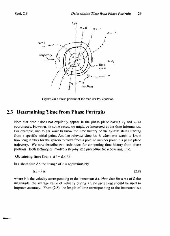
By taking a of different values, different isoclines can be obtained, as plotted in Figure 2.8.

Short line segments are drawn on the isoclines to generate a field of tangent directions. The phase

portraits can then be obtained, as shown in the plot. It is interesting to note that there exists a

closed curve in the portrait, and the trajectories starting from both outside and inside converge to

this curve. This closed curve corresponds to a limit cycle, as will be discussed further in section

2.5. •

Note that the same scales should be used for the xj axis and Xj axis of the phase

plane, so that the derivative dx^dx-^ equals the geometric slope of the trajectories.

Also note that, since in the second step of phase portrait construction we essentially

assume that the slope of the phase plane trajectories is locally constant, more isoclines

should be plotted in regions where the slope varies quickly, to improve accuracy.

Sect. 2.3 Determining Time from Phase Portraits 29

a = -5

a = l

trajectory

isoclines

Figure 2.8 : Phase portrait of the Van der Pol equation

2.3 Determining Time from Phase Portraits

Note that time t does not explicitly appear in the phase plane having Xy and x2 ascoordinates. However, in some cases, we might be interested in the time information.For example, one might want to know the time history of the system states startingfrom a specific initial point. Another relevant situation is when one wants to knowhow long it takes for the system to move from a point to another point in a phase planetrajectory. We now describe two techniques for computing time history from phaseportraits. Both techniques involve a step-by step procedure for recovering time.

Obtaining time from At~Ax/x

In a short time At, the change of x is approximately

Ax ~ xAt (2.8)

where x is the velocity corresponding to the increment Ax. Note that for a Ax of finitemagnitude, the average value of velocity during a time increment should be used toimprove accuracy. From (2.8), the length of time corresponding to the increment Ax


is

The above reasoning implies that, in order to obtain the time corresponding to themotion from one point to another point along a trajectory, one should divide thecorresponding part of the trajectory into a number of small segments (not necessarilyequally spaced), find the time associated with each segment, and then add up theresults. To obtain the time history of states corresponding to a certain initialcondition, one simply computes the time t for each point on the phase trajectory, andthen plots x with respect to t and x with respect to t,

Obtaining time from t = f (1/i) dx

Since x = dx/dt, we can write dt - dx/x. Therefore,

where x corresponds to time t and xo corresponds to time t0 . This equation impliesthat, if we plot a phase plane portrait with new coordinates x and (1/i), then the areaunder the resulting curve is the corresponding time interval.

2.4 Phase Plane Analysis of Linear Systems

In this section, we describe the phase plane analysis of linear systems. Besidesallowing us to visually observe the motion patterns of linear systems, this will alsohelp the development of nonlinear system analysis in the next section, because anonlinear systems behaves similarly to a linear system around each equilibrium point.

The general form of a linear second-order system is

xl=axr+ bx2 (2.9a)

k2 = cxi+dx2 (2.9b)

To facilitate later discussions, let us transform this equation into a scalar second-orderdifferential equation. Note from (2.9a) and (2.9b) that

b k2 = b cx\ + d(x\ — axj)

Consequently, differentiation of (2.9a) and then substitution of (2.9b) leads to

Sect. 2.4 Phase Plane Analysis of Linear Systems 31

Xj = (a +d)X\ + (cb - ad)xi

Therefore, we will simply consider the second-order linear system described by

x + ax + bx = 0 (2.10)

To obtain the phase portrait of this linear system, we first solve for the timehistory

x(t) = klexit + k2e

l2> forX,*^2 (2.11a)

x(t) = klexi' + k2tehl for X{ = X^ (2.11b)

where the constants X\ and X2 are the solutions of the characteristic equation

s2 + as + b = (s - A,j) (s - Xj) =0

The roots A,j and > can be explicitly represented as

For linear systems described by (2.10), there is only one singular point (assumingb & 0), namely the origin. However, the trajectories in the vicinity of this singularitypoint can display quite different characteristics, depending on the values of a and b.The following cases can occur

1. ^.j and Xj are both real and have the same sign (positive or negative)

2. X\ and Xj are both real and have opposite signs

3. A,j and X2 are complex conjugate with non-zero real parts

4. X{ and X2 are complex conjugates with real parts equal to zero

We now briefly discuss each of the above four cases.

STABLE OR UNSTABLE NODE

The first case corresponds to a node. A node can be stable or unstable. If theeigenvalues are negative, the singularity point is called a stable node because both x(f)and x(t) converge to zero exponentially, as shown in Figure 2.9(a). If botheigenvalues are positive, the point is called an unstable node, because both x(t) andx{t) diverge from zero exponentially, as shown in Figure 2.9(b). Since the eigenvaluesare real, there is no oscillation in the trajectories.


SADDLE POINT

The second case (say X^ < 0 and A > 0) corresponds to a saddle point (Figure 2.9(c)).The phase portrait of the system has the interesting "saddle" shape shown in Figure2.9(c). Because of the unstable pole Xj , almost all of the system trajectories divergeto infinity. In this figure, one also observes two straight lines passing through theorigin. The diverging line (with arrows pointing to infinity) corresponds to initialconditions which make £2 (i.e., the unstable component) equal zero. The convergingstraight line corresponds to initial conditions which make kl equal zero.

STABLE OR UNSTABLE FOCUS

The third case corresponds to a focus. A stable focus occurs when the real part of theeigenvalues is negative, which implies that x(t) and x(t) both converge to zero. Thesystem trajectories in the vicinity of a stable focus are depicted in Figure 2.9(d). Notethat the trajectories encircle the origin one or more times before converging to it,unlike the situation for a stable node. If the real part of the eigenvalues is positive,then x(t) and x(t) both diverge to infinity, and the singularity point is called anunstable focus. The trajectories corresponding to an unstable focus are sketched inFigure 2.9(e).

CENTER POINT

The last case corresponds to a center point, as shown in Figure 2.9(f). The namecomes from the fact that all trajectories are ellipses and the singularity point is thecenter of these ellipses. The phase portrait of the undamped mass-spring systembelongs to this category.

Note that the stability characteristics of linear systems are uniquely determinedby the nature of their singularity points. This, however, is not true for nonlinearsystems.

2.5 Phase Plane Analysis of Nonlinear Systems

In discussing the phase plane analysis of nonlinear systems, two points should be keptin mind. Phase plane analysis of nonlinear systems is related to that of linear systems,because the local behavior of a nonlinear system can be approximated by the behaviorof a linear system. Yet, nonlinear systems can display much more complicatedpatterns in the phase plane, such as multiple equilibrium points and limit cycles. Wenow discuss these points in more detail.

Sect. 2.5 Phase Plane Analysis of Nonlinear Systems 33

stable node

(a)

11

unstable nodeX X - C7

(b)77

saddle point

(c)

stable focus

(d)

unstable focus

x

(e)

center point

(0

Figure 2.9 : Phase-portraits of linear systems


LOCAL BEHAVIOR OF NONLINEAR SYSTEMS

In the phase portrait of Figure 2.2, one notes that, in contrast to linear systems, thereare two singular points, (0,0) and (-3,0) . However, we also note that the features ofthe phase trajectories in the neighborhood of the two singular points look very muchlike those of linear systems, with the first point corresponding to a stable focus and thesecond to a saddle point. This similarity to a linear system in the local region of eachsingular point can be formalized by linearizing the nonlinear system, as we nowdiscuss.

If the singular point of interest is not at the origin, by defining the differencebetween the original state and the singular point as a new set of state variables, onecan always shift the singular point to the origin. Therefore, without loss of generality,we may simply consider Equation (2.1) with a singular point at 0. Using Taylorexpansion, Equations (2.1a) and (2.1b) can be rewritten as

h = c x l + dx2 + 82^1 ' X2>

where gj and g2 contain higher order terms.

In the vicinity of the origin, the higher order terms can be neglected, andtherefore, the nonlinear system trajectories essentially satisfy the linearized equation

JL'j = axl + bx2

x2 = cxi+dx2

As a result, the local behavior of the nonlinear system can be approximated by thepatterns shown in Figure 2.9.

LIMIT CYCLES

m the phase portrait of the nonlinear Van der Pol equation, shown in Figure 2.8, oneobserves that the system has an unstable node at the origin. Furthermore, there is aclosed curve in the phase portrait. Trajectories inside the curve and those outside thecurve all tend to this curve, while a motion started on this curve will stay on it forever,circling periodically around the origin. This curve is an instance of the so-called"limit cycle" phenomenon. Limit cycles are unique features of nonlinear systems.

In the phase plane, a limit cycle is defined as an isolated closed curve. Thetrajectory has to be both closed, indicating the periodic nature of the motion, andisolated, indicating the limiting nature of the cycle (with nearby trajectories

Sect. 2.5 Phase Plane Analysis of Nonlinear Systems 35

converging or diverging from it). Thus, while there are many closed curves in thephase portraits of the mass-spring-damper system in Example 2.1 or the satellitesystem in Example 2.5, these are not considered limit cycles in this definition, becausethey are not isolated.

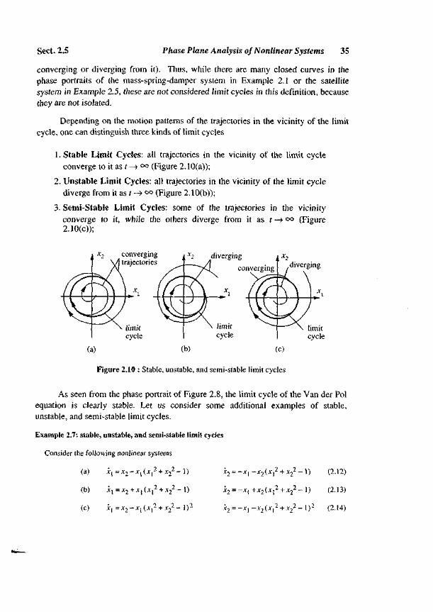
Depending on the motion patterns of the trajectories in the vicinity of the limitcycle, one can distinguish three kinds of limit cycles

1. Stable Limit Cycles: all trajectories in the vicinity of the limit cycleconverge to it as t —> °° (Figure 2.10(a));

2. Unstable Limit Cycles: all trajectories in the vicinity of the limit cyclediverge from it as t -> °° (Figure 2.10(b));

3. Semi-Stable Limit Cycles: some of the trajectories in the vicinityconverge to it, while the others diverge from it as r —» °° (Figure

2 divergingconverging diverging

(a) (b) (c)

Figure 2.10 : Stable, unstable, and semi-stable limit cycles

As seen from the phase portrait of Figure 2.8, the limit cycle of the Van der Polequation is clearly stable. Let us consider some additional examples of stable,unstable, and semi-stable limit cycles.

Example 2.7: stable, unstable, and semi-stable limit cycles

Consider the following nonlinear systems

(a)

(b)

(c)

l=x2-xx(xl

X , = J

- I)2

-x2(xf

+x2(x,2

-x2(x,2

+ x 2 - -

+ x 22 -

+ x 22 -

1)

I ) 2

(2.12)

(2.13)

(2.14)


Let us study system (a) first. By introducing polar coordinates

/• = (x 12 + x2

2)1/2 9 = tan-1(jc2/x1)

the dynamic equations (2.12) are transformed as

dr , , , . d<d

T<=-r(r-l) Tr-X

When the state starts on the unit circle, the above equation shows that r(t) = 0. Therefore, the state

will circle around the origin with a period 1/2K. When r < 1, then r > 0. This implies that the state

tends to the circle from inside. When r > 1, then /• < 0. This implies that the state tends toward

the unit circle from outside. Therefore, the unit circle is a stable limit cycle. This can also be

concluded by examining the analytical solution of (2.12)

r(t) = 1 6(0 = Qn - 1( l+c oe- 2 ' ) 1 / 2

where

Similarly, one can find that the system (b) has an unstable limit cycle and system (c) has a semi-

stable limit cycle. Q

2.6 Existence of Limit Cycles

As mentioned in chapter 1, it is of great importance for control engineers to predict theexistence of limit cycles in control systems. In this section, we state three simpleclassical theorems to that effect. These theorems are easy to understand and apply.

The first theorem to be presented reveals a simple relationship between theexistence of a limit cycle and the number of singular points it encloses. In thestatement of the theorem, we use N to represent the number of nodes, centers, and focienclosed by a limit cycle, and S to represent the number of enclosed saddle points.

Theorem 2.1 (Poincare) / / a limit cycle exists in the second-order autonomoussystem (2.1), then N = S + 1 .

This theorem is sometimes called the index theorem. Its proof is mathematicallyinvolved (actually, a family of such proofs led to the development of algebraictopology) and shall be omitted here. One simple inference from this theorem is that alimit cycle must enclose at least one equilibrium point. The theorem's result can be

Sect. 2.6 Existence of Limit Cycles 37

verified easily on Figures 2.8 and 2.10.

The second theorem is concerned with the asymptotic properties of thetrajectories of second-order systems.

Theorem 2.2 (Poincare-Bendixson) If a trajectory of the second-orderautonomous system remains in a finite region Q, then one of the following is true:

(a) the trajectory goes to an equilibrium point

(b) the trajectory tends to an asymptotically stable limit cycle

(c) the trajectory is itself a limit cycle

While the proof of this theorem is also omitted here, its intuitive basis is easy to see,and can be verified on the previous phase portraits.

The third theorem provides a sufficient condition for the non-existence of limitcycles.

Theorem 2.3 (Bendixson) For the nonlinear system (2.1), no limit cycle can existin a region Q. of the phase plane in which 3/j /3xj + 3/2/3.X2 does not vanish anddoes not change sign.

Proof: Let us prove this theorem by contradiction. First note that, from (2.5), the equation

0 (2.15)

is satisfied for any system trajectories, including a limit cycle. Thus, along the closed curve L of

a limit cycle, we have

f (/,rfjc2-/2rfx-1> = 0 (2.16)

Using Stokes' Theorem in calculus, we have

where the integration on the right-hand side is carried out on the area enclosed by the limit cycle.

By Equation (2.16), the left-hand side must equal zero. This, however, contradicts the fact

that the right-hand side cannot equal zero because by hypothesis 3/j/3xj +3/2 /3x2 does not

vanish and does not change sign. El

Let us illustrate the result on an example.


Example 2.8: Consider the nonlinear system

x2 =

Since

which is always strictly positive (except at the origin), the system does not have any limit cycles

anywhere in the phase plane. . \3

The above three theorems represent very powerful results. It is important tonotice, however, that they have no equivalent in higher-order systems, where exoticasymptotic behaviors other than equilibrium points and limit cycles can occur.

2.7 Summary

Phase plane analysis is a graphical method used to study second-order dynamicsystems. The major advantage of the method is that it allows visual examination of theglobal behavior of systems. The major disadvantage is that it is mainly limited tosecond-order systems (although extensions to third-order systems are often achievedwith the aid of computer graphics). The phenomena of multiple equilibrium points andof limit cycles are clearly seen in phase plane analysis. A number of useful classicaltheorems for the prediction of limit cycles in second-order systems are also presented.

2.8 Notes and References

Phase plane analysis is a very classical topic which has been addressed by numerous control texts.

An extensive treatment can be found in [Graham and McRuer, 1961]. Examples 2.2 and 2.3 are

adapted from [Ogata, 1970]. Examples 2.5 and 2.6 and section 2.6 are based on [Hsu and Meyer,

1968].

2.9 Exercises

2.1 Draw the phase portrait and discuss the properties of the linear, unity feedback control system

of open-loop transfer function

1 0

Sect. 2.9

2.2 Draw the phase portraits of the following systems, using isoclines

(a) e + e + 0.5 e = o

(b) e + e + o.5 e = i

Exercises 39

2.3 Consider the nonlinear system

x = y + x(x* + yl- 1) sin

y = - x + y (x2 + y2 - 1) sin

Without solving the above equations explicitly, show that the system has infinite number of limit

cycles. Determine the stability of these limit cycles. (Hint: Use polar coordinates.)

2.4 The system shown in Figure 2.10 represents a satellite control system with rate feedback

provided by a gyroscope. Draw the phase portrait of the system, and determine the system's

stability.

p + a -1 'u 1

P1

Figure 2.10 : Satellite control system with rate feedback

Chapter 2 Phase Plane Analysis - WordPress.com · Chapter 2 Phase Plane Analysis Phase plane...

Documents

Transcript of Chapter 2 Phase Plane Analysis - WordPress.com · Chapter 2 Phase Plane Analysis Phase plane...