CHAPTER 2: PARTICLE IN A CENTRAL POTENTIAL.THE HYDROGEN ATOM

(From Cohen-Tannoudji, Chapter VII)

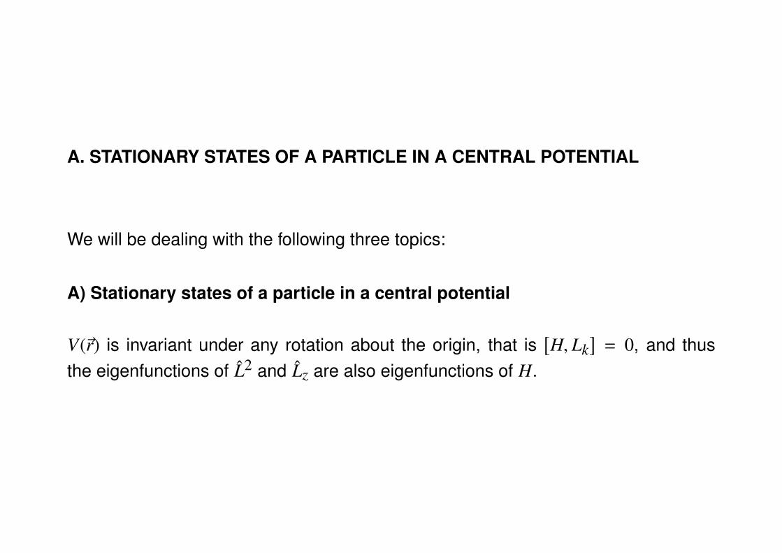
A. STATIONARY STATES OF A PARTICLE IN A CENTRAL POTENTIAL

We will be dealing with the following three topics:

A) Stationary states of a particle in a central potential

V(~r) is invariant under any rotation about the origin, that is[H, Lk

]= 0, and thus

the eigenfunctions of L2 and Lz are also eigenfunctions of H.

B) Motion of the center of mass and relative motion for a system of two inter-acting particles

(i) a two particle system in which interaction energy depends only on the particles’relative position can be replaced by a simpler problem of one fictitious particle;

(ii) in addition, when the interaction depends only on the distance between parti-cles, then the fictitious particle’s motion is governed by a central potential.

C) Exactly solvable problems

(i) V(~r) is a Coulomb potential: hydrogen, deuterium, tritium, He+,Li+;

(ii) V(~r) is a quadratic potential: isotropic three-dimensional harmonic oscillator.

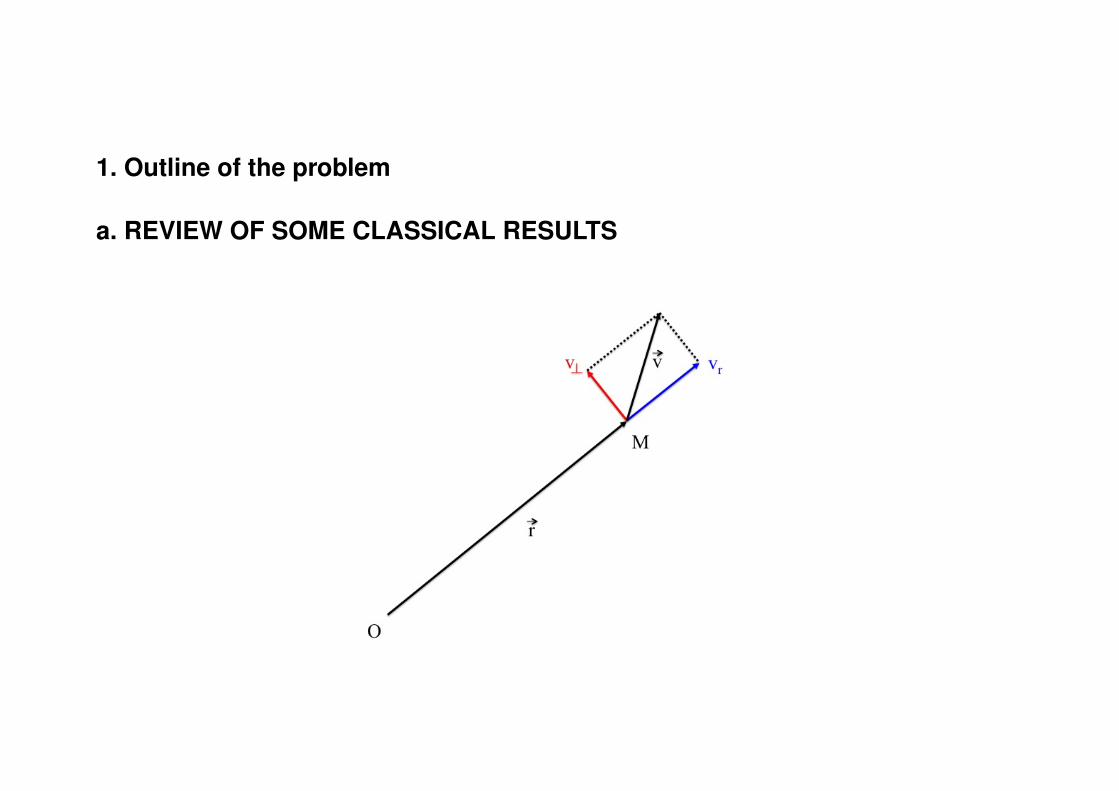
1. Outline of the problem

a. REVIEW OF SOME CLASSICAL RESULTS

Force on the particle located at the point M

~F = −~∇V(r) = −dVdr~rr

(2.1)

is always directed to the origin O. In this case the angular momentum theoremimplies that the angular momentum ~L = ~r × ~p is a constant of motion:

d ~Ldt

= ~0 (2.2)

and the particle trajectory is on the plane through the origin and perpendicular to ~L.

Let us consider now the position and velocity of the particle at time t. The velocitycan be decomposed into the radial vr and tangential velocity ~v⊥ defined through therelations

vr =drdt

(2.3)

∣∣∣~r × ~v∣∣∣ = r∣∣∣~v⊥∣∣∣ (2.4)

so that the modulus of the angular momentum is given as∣∣∣∣ ~L∣∣∣∣ =∣∣∣~r × µ~v∣∣∣ = µr

∣∣∣~v⊥∣∣∣ (2.5)

The total energy of the particle

E =12µ~v2 + V(r) =

12µ~v2

r +12µ~v2⊥ + V(r) (2.6)

can be rewritten as

E =12µv2

r +~L2

2µr2 + V(r) (2.7)

which follows from

~L2 =∣∣∣∣ ~L2

∣∣∣∣ = µ2r2 ∣∣∣~v⊥∣∣∣2 = r2p2⊥ (2.8)

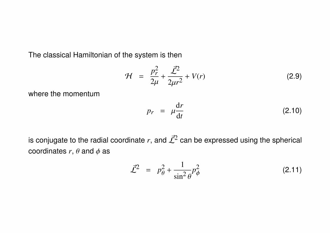
The classical Hamiltonian of the system is then

H =p2

r2µ

+~L2

2µr2 + V(r) (2.9)

where the momentum

pr = µdrdt

(2.10)

is conjugate to the radial coordinate r, and ~L2 can be expressed using the sphericalcoordinates r, θ and φ as

~L2 = p2θ +

1

sin2 θp2φ (2.11)

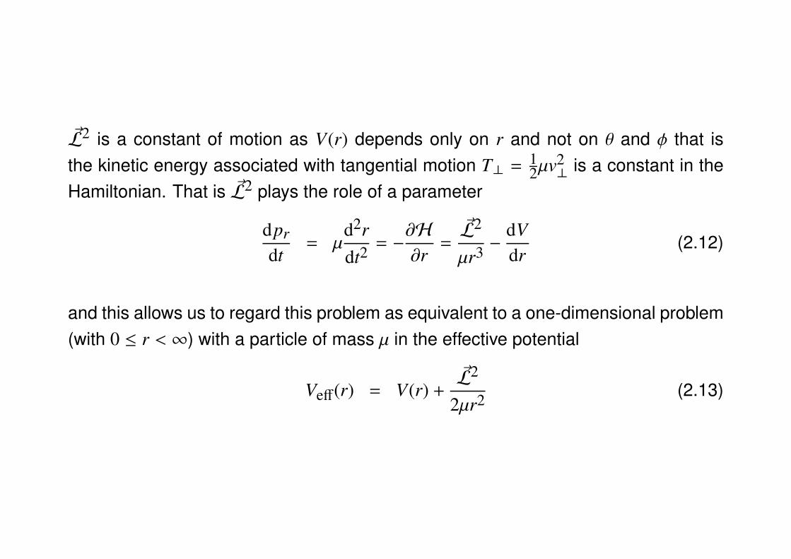
~L2 is a constant of motion as V(r) depends only on r and not on θ and φ that isthe kinetic energy associated with tangential motion T⊥ = 1

2µv2⊥ is a constant in the

Hamiltonian. That is ~L2 plays the role of a parameter

dprdt

= µd2rdt2

= −∂H

∂r=

~L2

µr3 −dVdr

(2.12)

and this allows us to regard this problem as equivalent to a one-dimensional problem(with 0 ≤ r < ∞) with a particle of mass µ in the effective potential

Veff(r) = V(r) +~L2

2µr2 (2.13)

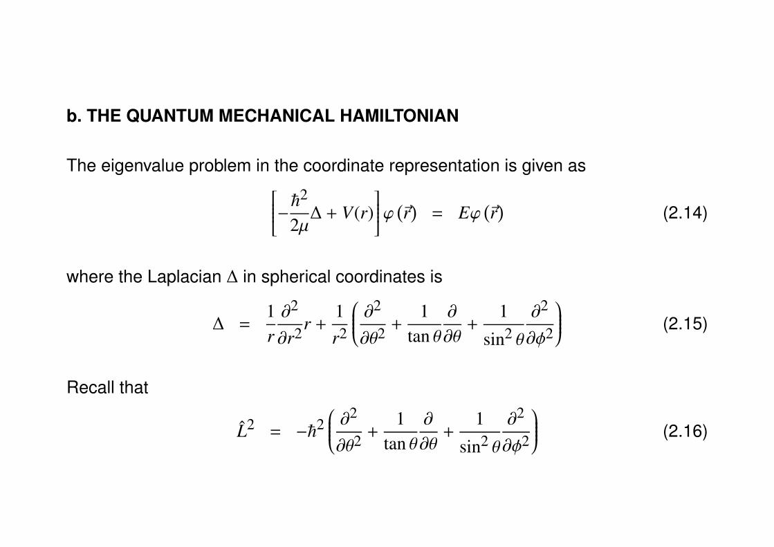
b. THE QUANTUM MECHANICAL HAMILTONIAN

The eigenvalue problem in the coordinate representation is given as−~22µ∆ + V(r)

ϕ (~r)

= Eϕ(~r)

(2.14)

where the Laplacian ∆ in spherical coordinates is

∆ =1r∂2

∂r2r +1r2

∂2

∂θ2 +1

tan θ∂

∂θ+

1

sin2 θ

∂2

∂φ2

(2.15)

Recall that

L2 = −~2 ∂2

∂θ2 +1

tan θ∂

∂θ+

1

sin2 θ

∂2

∂φ2

(2.16)

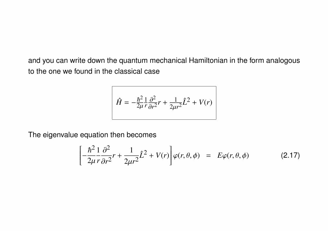
and you can write down the quantum mechanical Hamiltonian in the form analogousto the one we found in the classical case

H = −~2

2µ1r∂2

∂r2r + 12µr2 L2 + V(r)

The eigenvalue equation then becomes−~22µ1r∂2

∂r2r +1

2µr2 L2 + V(r)ϕ(r, θ, φ) = Eϕ(r, θ, φ) (2.17)

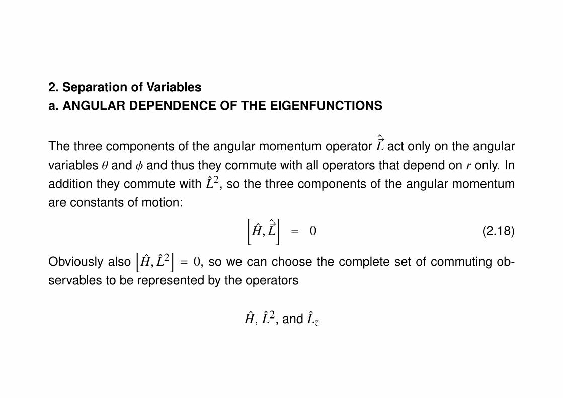
2. Separation of Variablesa. ANGULAR DEPENDENCE OF THE EIGENFUNCTIONS

The three components of the angular momentum operator ~L act only on the angularvariables θ and φ and thus they commute with all operators that depend on r only. Inaddition they commute with L2, so the three components of the angular momentumare constants of motion: [

H, ~L]

= 0 (2.18)

Obviously also[H, L2

]= 0, so we can choose the complete set of commuting ob-

servables to be represented by the operators

H, L2, and Lz

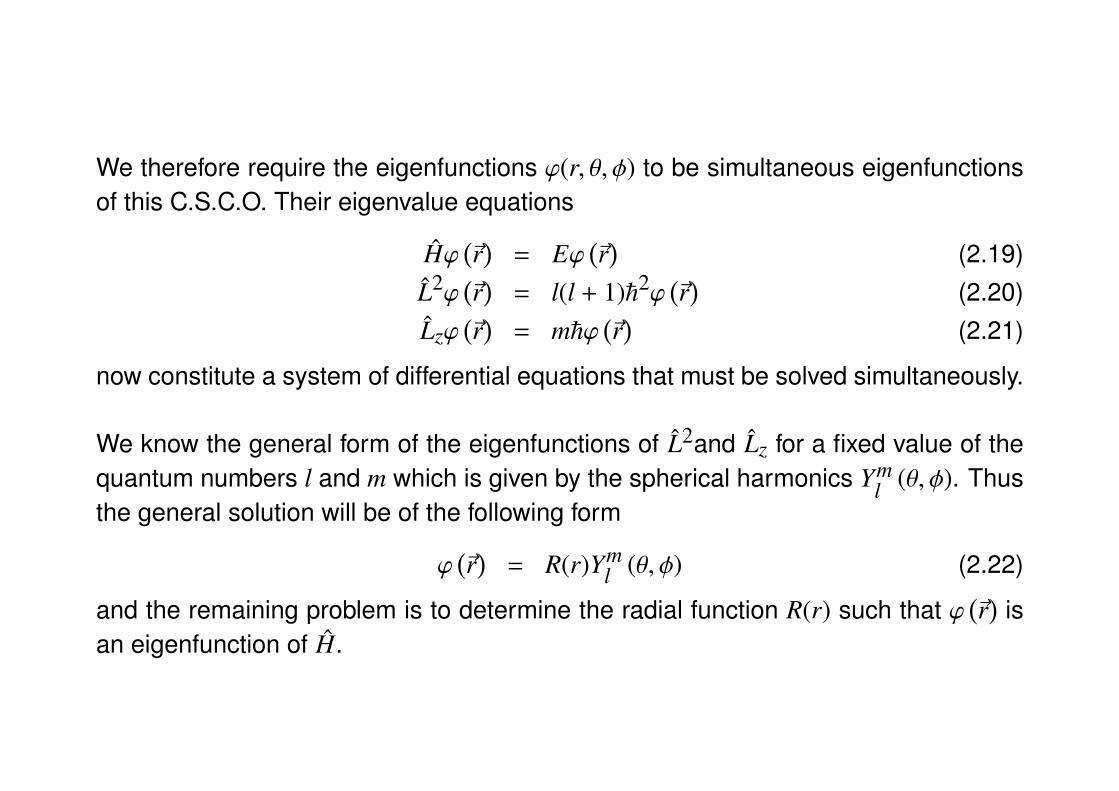
We therefore require the eigenfunctions ϕ(r, θ, φ) to be simultaneous eigenfunctionsof this C.S.C.O. Their eigenvalue equations

Hϕ(~r)

= Eϕ(~r)

(2.19)L2ϕ

(~r)

= l(l + 1)~2ϕ(~r)

(2.20)Lzϕ

(~r)

= m~ϕ(~r)

(2.21)

now constitute a system of differential equations that must be solved simultaneously.

We know the general form of the eigenfunctions of L2and Lz for a fixed value of thequantum numbers l and m which is given by the spherical harmonics Ym

l (θ, φ). Thusthe general solution will be of the following form

ϕ(~r)

= R(r)Yml (θ, φ) (2.22)

and the remaining problem is to determine the radial function R(r) such that ϕ(~r)

isan eigenfunction of H.

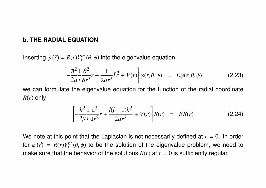
b. THE RADIAL EQUATION

Inserting ϕ(~r)

= R(r)Yml (θ, φ) into the eigenvalue equation−~22µ

1r∂2

∂r2r +1

2µr2 L2 + V(r)ϕ(r, θ, φ) = Eϕ(r, θ, φ) (2.23)

we can formulate the eigenvalue equation for the function of the radial coordinateR(r) only −~22µ

1r

d2

dr2r +l(l + 1)~2

2µr2 + V(r) R(r) = ER(r) (2.24)

We note at this point that the Laplacian is not necessarily defined at r = 0. In orderfor ϕ

(~r)

= R(r)Yml (θ, φ) to be the solution of the eigenvalue problem, we need to

make sure that the behavior of the solutions R(r) at r = 0 is sufficiently regular.

Now we face the eigenvalue problem, i.e. represented by a differential equation,which depends only on r and l as parameters, i.e. we are looking for eigenvaluesand eigenvectors of Hl which is different for different values of l.

In the state space E~r, we consider subspaces E(l,m) for fixed values of l and m, andstudy the eigenvalue equation of H in each of these subspaces:

- the equation is the same in the (2l + 1) subspaces E(l,m) associated with l;

- Ek,l are eigenvalues of Hl in a given E(l,m), and they can be discrete or continuousdepending on k which represents various eigenvalues with the same value of l;

- Rk,l(r) are eigenfunctions of Hl in E(l,m).

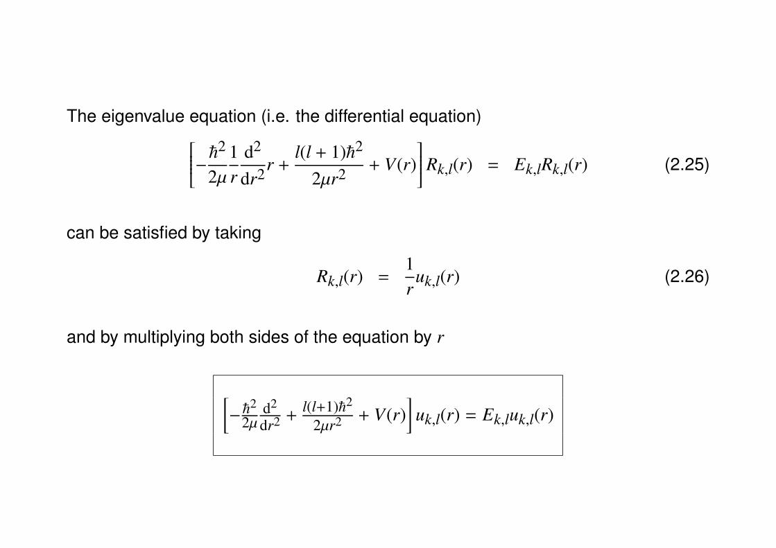
The eigenvalue equation (i.e. the differential equation)−~22µ1r

d2

dr2r +l(l + 1)~2

2µr2 + V(r) Rk,l(r) = Ek,lRk,l(r) (2.25)

can be satisfied by taking

Rk,l(r) =1r

uk,l(r) (2.26)

and by multiplying both sides of the equation by r

[−~

2

2µd2

dr2 +l(l+1)~2

2µr2 + V(r)]

uk,l(r) = Ek,luk,l(r)

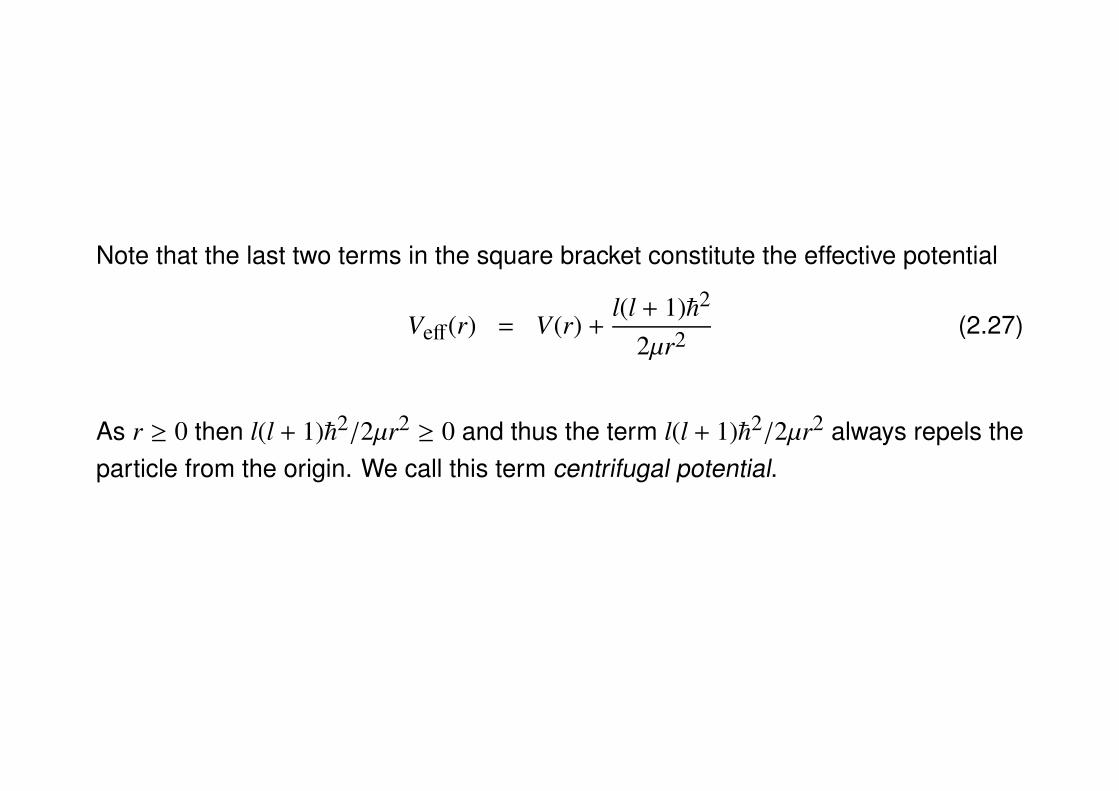
Note that the last two terms in the square bracket constitute the effective potential

Veff(r) = V(r) +l(l + 1)~2

2µr2 (2.27)

As r ≥ 0 then l(l + 1)~2/2µr2 ≥ 0 and thus the term l(l + 1)~2/2µr2 always repels theparticle from the origin. We call this term centrifugal potential.

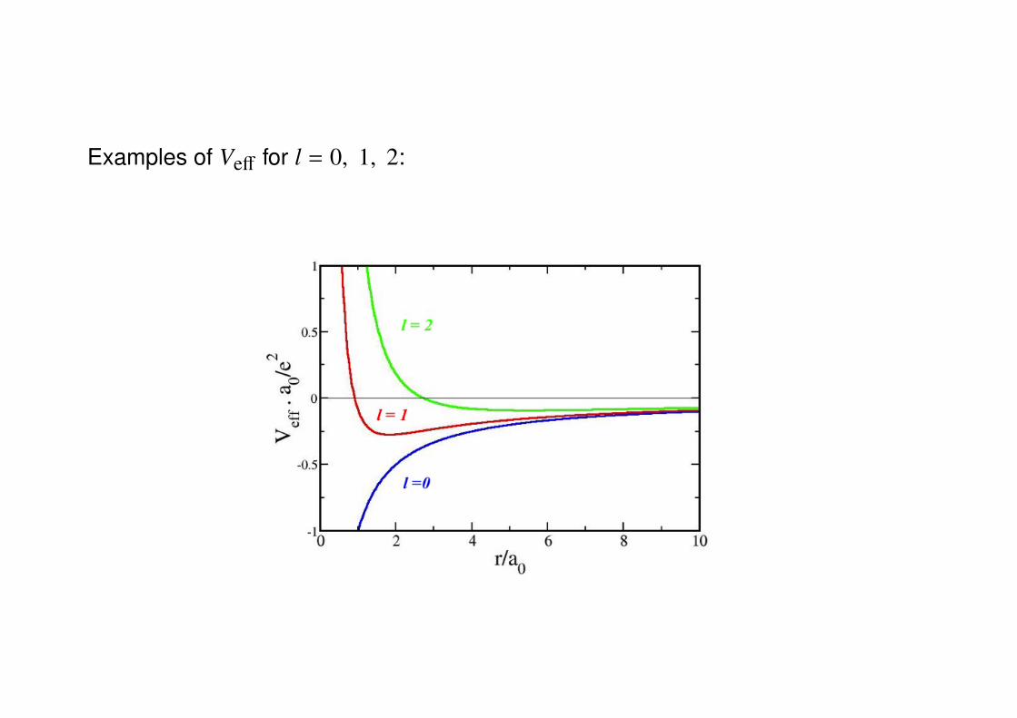
Examples of Veff for l = 0, 1, 2:

c. BEHAVIOR OF THE SOLUTIONS OF THE RADIAL EQUATION AT THE ORIGIN

We have to examine the behavior of R(r) at r = 0 to know whether they really aresolutions of the eigenvalue problem. We assume

• V(r) is for r → 0 either finite or approaches infinity less rapidly than 1r ;

• for r → 0 the radial function Rk,l(r) ∼ Crs

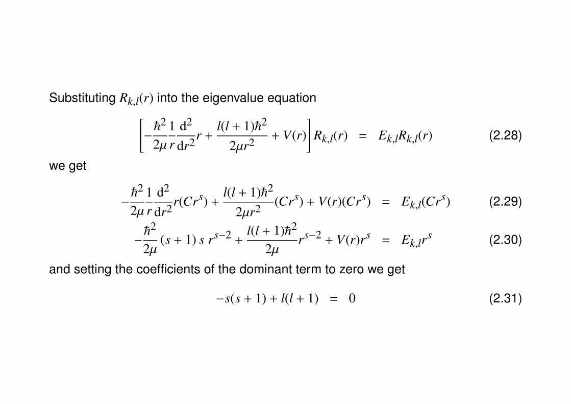
Substituting Rk,l(r) into the eigenvalue equation−~22µ1r

d2

dr2r +l(l + 1)~2

2µr2 + V(r) Rk,l(r) = Ek,lRk,l(r) (2.28)

we get

−~2

2µ1r

d2

dr2r(Crs) +l(l + 1)~2

2µr2 (Crs) + V(r)(Crs) = Ek,l(Crs) (2.29)

−~2

2µ(s + 1) s rs−2 +

l(l + 1)~2

2µrs−2 + V(r)rs = Ek,lr

s (2.30)

and setting the coefficients of the dominant term to zero we get

−s(s + 1) + l(l + 1) = 0 (2.31)

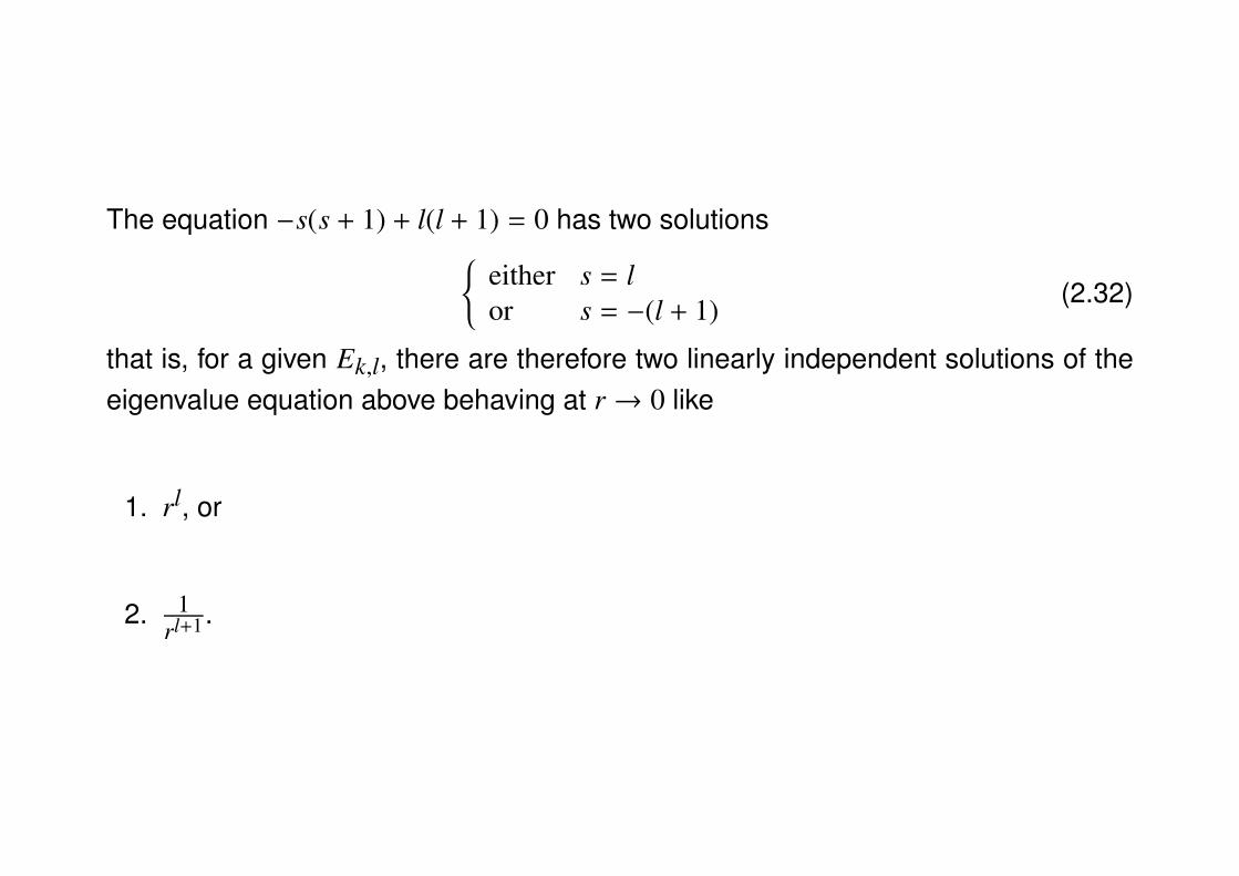
The equation −s(s + 1) + l(l + 1) = 0 has two solutionseither s = lor s = −(l + 1) (2.32)

that is, for a given Ek,l, there are therefore two linearly independent solutions of theeigenvalue equation above behaving at r → 0 like

1. rl, or

2. 1rl+1 .

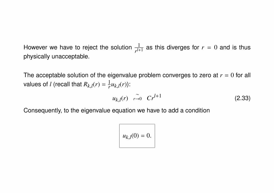
However we have to reject the solution 1rl+1 as this diverges for r = 0 and is thus

physically unacceptable.

The acceptable solution of the eigenvalue problem converges to zero at r = 0 for allvalues of l (recall that Rk,l(r) = 1

r uk,l(r)):

uk,l(r)∼

r→0 Crl+1 (2.33)

Consequently, to the eigenvalue equation we have to add a condition

uk,l(0) = 0.

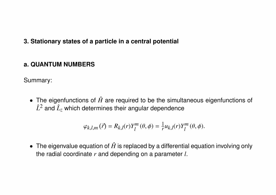
3. Stationary states of a particle in a central potential

a. QUANTUM NUMBERS

Summary:

• The eigenfunctions of H are required to be the simultaneous eigenfunctions ofL2 and Lz which determines their angular dependence

ϕk,l,m(~r)

= Rk,l(r)Yml (θ, φ) = 1

r uk,l(r)Yml (θ, φ).

• The eigenvalue equation of H is replaced by a differential equation involving onlythe radial coordinate r and depending on a parameter l.

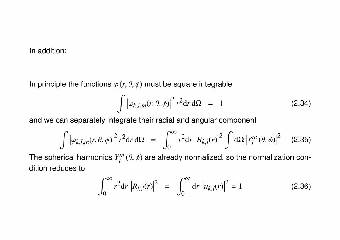
In addition:

In principle the functions ϕ (r, θ, φ) must be square integrable∫ ∣∣∣ϕk,l,m(r, θ, φ)∣∣∣2 r2dr dΩ = 1 (2.34)

and we can separately integrate their radial and angular component∫ ∣∣∣ϕk,l,m(r, θ, φ)∣∣∣2 r2dr dΩ =

∫ ∞0

r2dr∣∣∣Rk,l(r)

∣∣∣2 ∫dΩ

∣∣∣Yml (θ, φ)

∣∣∣2 (2.35)

The spherical harmonics Yml (θ, φ) are already normalized, so the normalization con-

dition reduces to ∫ ∞0

r2dr∣∣∣Rk,l(r)

∣∣∣2 =

∫ ∞0

dr∣∣∣uk,l(r)

∣∣∣2 = 1 (2.36)

We note that if the spectrum has a continuous part, i.e. k is a continuous index, then∫ ∞0

r2dr R∗k′,l(r)Rk,l(r) =

∫ ∞0

dr u∗k′,l(r)uk,l(r) = δ(k′ − k

)(2.37)

where δ(k′ − k

)is δ-function. Since this is not a square integrable function, the nor-

malization integral diverges for k = k′.

An eigenfunction

ϕk,l,m(~r)

= Rk,l(r)Yml (θ, φ)

depends on three parameters as it is a simultaneous eigenfunction of H, L2 and Lzwith eigenvalues Ek, l(l + 1)~2, and m~.

We call these parameters - k, l and m - quantum numbers:

k - a radial quantum number,l - an azimuthal quantum number,m - a magnetic quantum number.

The radial part Rk,l(r) = 1r uk,l(r) of ϕk,l,m

(~r)

are independent of m and are given bythe eigenvalue equation

[−~

2

2µd2

dr2 +l(l+1)~2

2µr2 + V(r)]

uk,l(r) = Ek,luk,l(r)

The angular part depends only on l and m, and it does NOT depend on the form ofthe potential V(r).

b. DEGENERACY OF THE ENERGY LEVELS

(2l + 1) orthogonal functions ϕk,l,m(~r)

with k and l fixed and m varying from −l to +lare eigenfunctions of H with the same eigenvalue Ek,l.

That is Ek,l is at least (2l + 1)-fold degenerate. This is called essential degeneracyas it exists for all V(r) and is due to the fact that H depends on L2 but not on Lz.

It is also possible that Ek,l = Ek′,l′ for l , l′. This occurs for certain potentials and itis called accidental degeneracy.

Remarks:

For a fixed l, the radial equation has at most one solution which is physically accept-able. This is ensured by the condition uk,l(0) = 0.

The behavior of the solutions as r → ∞ follows from the behavior of the potentialV(r → ∞)→ 0. The negative values of Ek,l form a discrete set.

B. MOTION OF THE CENTER OF MASS AND RELATIVE MOTION FOR A SYS-TEM OF TWO INTERACTING PARTICLES

1. Motion of the center of mass and relative motion in classical mechanics

Let us consider two spinless particles with masses m1 and m2 and positions ~r1 and~r2 respectively, and assume that the force between the particles is derived from thepotential V(r) = V(~r1 − ~r2).

in classical mechanics the system is described by the Lagrangian

£(~r1, ~r1;~r2, ~r2

)= T − V =

12

m1~r21 +

12

m2~r22 − V

(~r1 − ~r2

). (2.38)

The momental of the particles are

~p1 = m1~r1 (2.39)

~p2 = m2~r2 (2.40)

The study of the motion of the two particles is simplified by introducing(i) center of mass coordinates

~rG =m1~r1 + m2~r2

m1 + m2(2.41)

(ii) relative coordinates

~r = ~r1 − ~r2 (2.42)

where

~r1 = ~rG +m2

m1 + m2~r (2.43)

~r2 = ~rG −m1

m1 + m2~r (2.44)

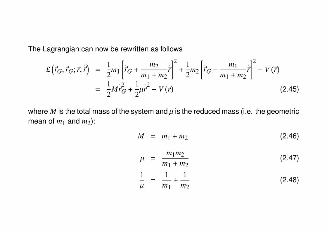
The Lagrangian can now be rewritten as follows

£(~rG, ~rG;~r, ~r

)=

12

m1

[~rG +

m2m1 + m2

~r]2

+12

m2

[~rG −

m1m1 + m2

~r]2− V

(~r)

=12

M~r2G +

12µ~r

2− V

(~r)

(2.45)

where M is the total mass of the system and µ is the reduced mass (i.e. the geometricmean of m1 and m2):

M = m1 + m2 (2.46)

µ =m1m2

m1 + m2(2.47)

1µ

=1

m1+

1m2

(2.48)

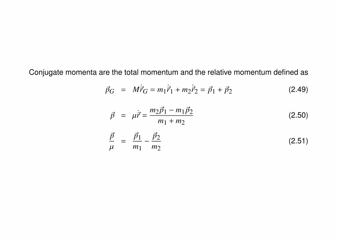
Conjugate momenta are the total momentum and the relative momentum defined as

~pG = M~rG = m1~r1 + m2~r2 = ~p1 + ~p2 (2.49)

~p = µ~r =m2~p1 − m1~p2

m1 + m2(2.50)

~pµ

=~p1m1−~p2m2

(2.51)

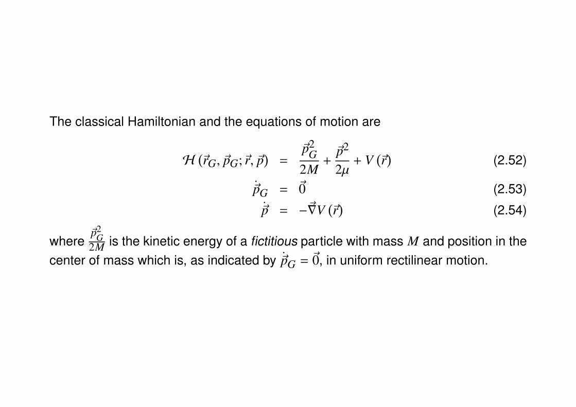
The classical Hamiltonian and the equations of motion are

H(~rG, ~pG;~r, ~p

)=

~p2G

2M+~p2

2µ+ V

(~r)

(2.52)

~pG = ~0 (2.53)

~p = −~∇V(~r)

(2.54)

where~p2

G2M is the kinetic energy of a fictitious particle with mass M and position in the

center of mass which is, as indicated by ~pG = ~0, in uniform rectilinear motion.

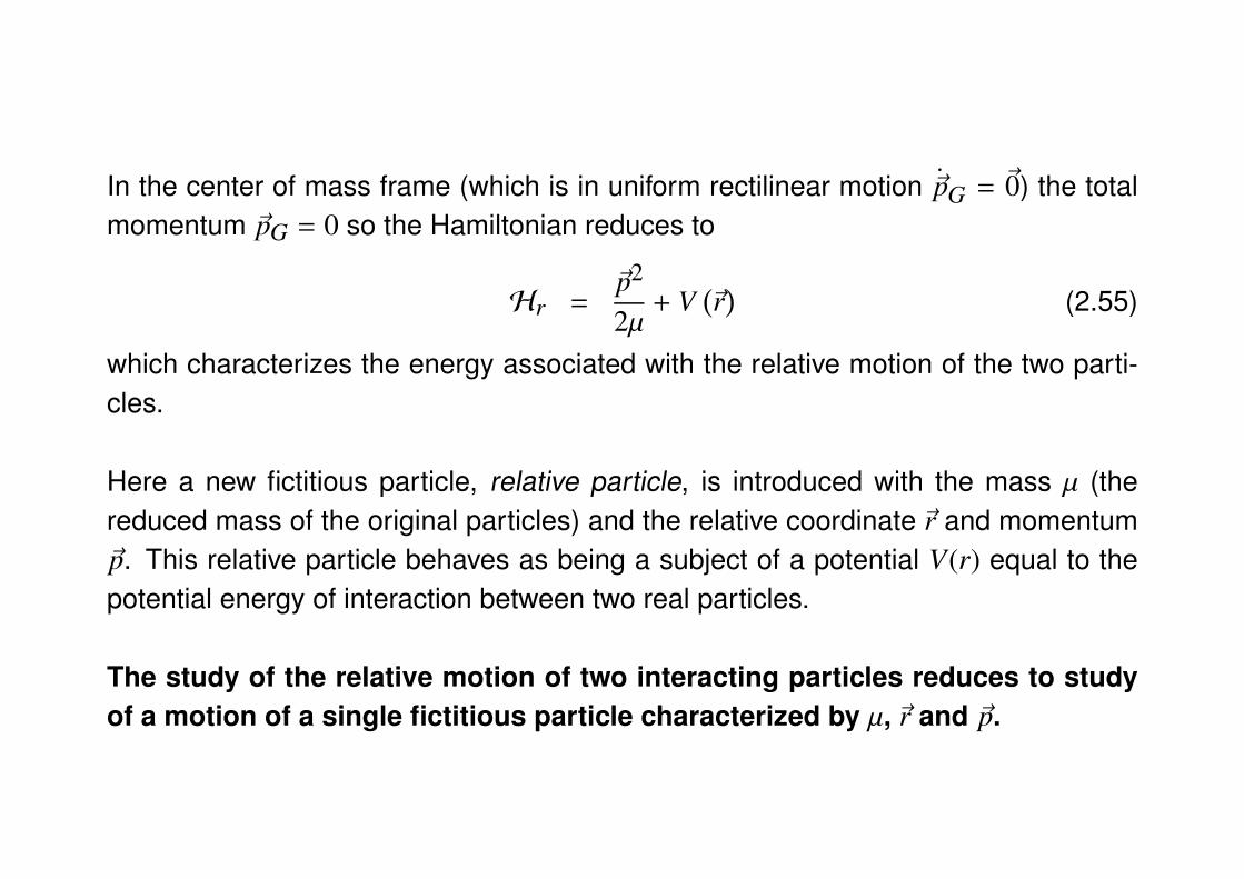
In the center of mass frame (which is in uniform rectilinear motion ~pG = ~0) the totalmomentum ~pG = 0 so the Hamiltonian reduces to

Hr =~p2

2µ+ V

(~r)

(2.55)

which characterizes the energy associated with the relative motion of the two parti-cles.

Here a new fictitious particle, relative particle, is introduced with the mass µ (thereduced mass of the original particles) and the relative coordinate ~r and momentum~p. This relative particle behaves as being a subject of a potential V(r) equal to thepotential energy of interaction between two real particles.

The study of the relative motion of two interacting particles reduces to studyof a motion of a single fictitious particle characterized by µ, ~r and ~p.

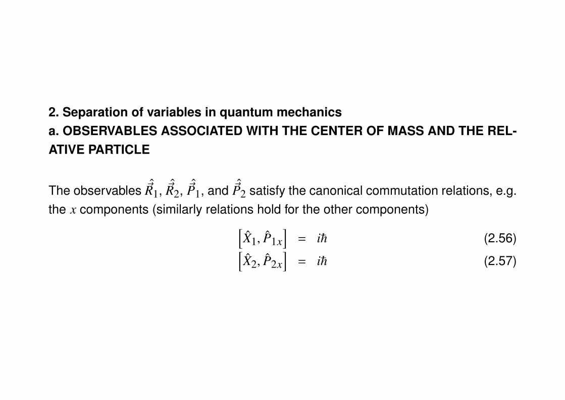
2. Separation of variables in quantum mechanicsa. OBSERVABLES ASSOCIATED WITH THE CENTER OF MASS AND THE REL-ATIVE PARTICLE

The observables ~R1, ~R2, ~P1, and ~P2 satisfy the canonical commutation relations, e.g.the x components (similarly relations hold for the other components)[

X1, P1x]

= i~ (2.56)[X2, P2x

]= i~ (2.57)

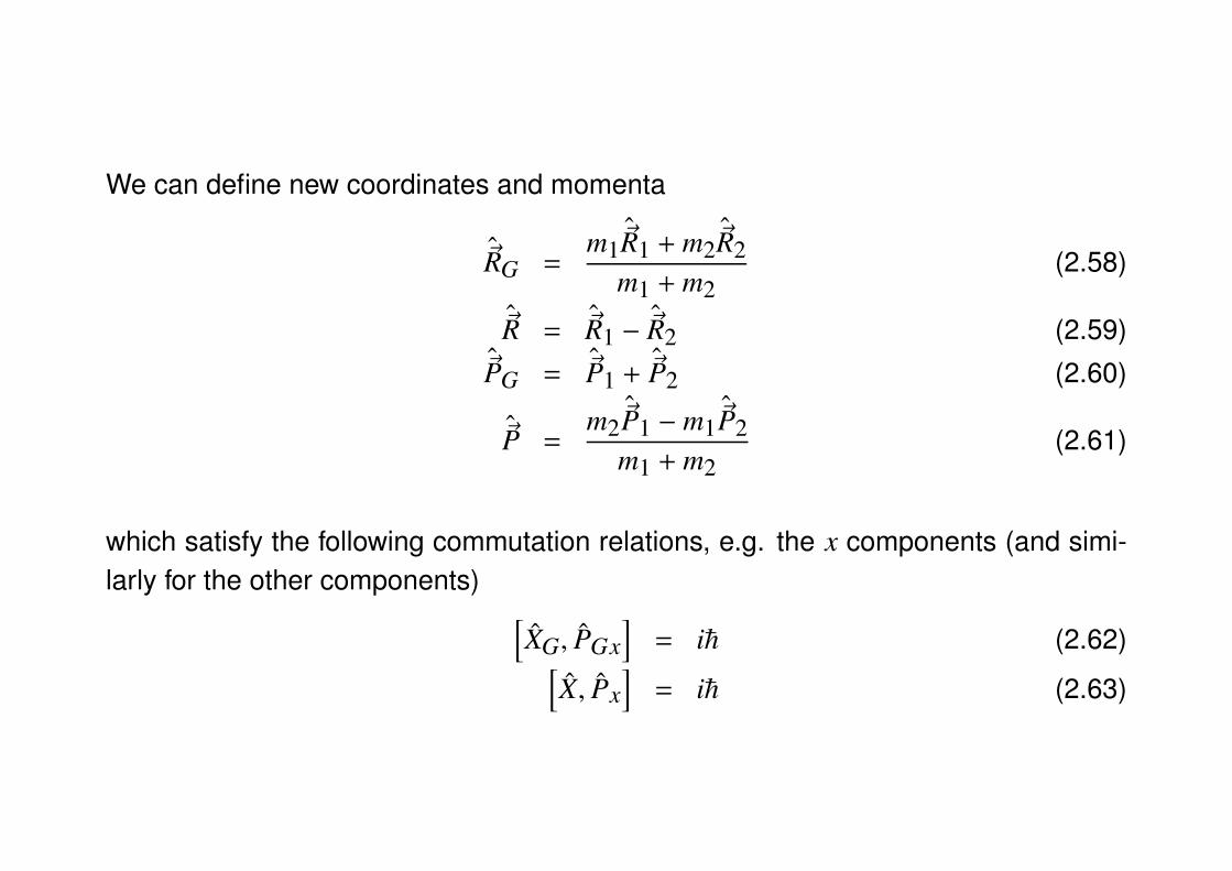
We can define new coordinates and momenta

~RG =m1 ~R1 + m2 ~R2

m1 + m2(2.58)

~R = ~R1 − ~R2 (2.59)~PG = ~P1 + ~P2 (2.60)

~P =m2 ~P1 − m1 ~P2

m1 + m2(2.61)

which satisfy the following commutation relations, e.g. the x components (and simi-larly for the other components) [

XG, PGx]

= i~ (2.62)[X, Px

]= i~ (2.63)

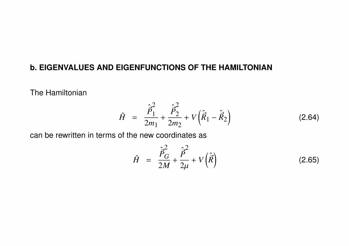
b. EIGENVALUES AND EIGENFUNCTIONS OF THE HAMILTONIAN

The Hamiltonian

H =~P

21

2m1+

~P22

2m2+ V

(~R1 − ~R2

)(2.64)

can be rewritten in terms of the new coordinates as

H =~P

2G

2M+~P

2

2µ+ V

(~R)

(2.65)

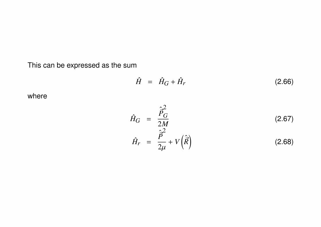
This can be expressed as the sum

H = HG + Hr (2.66)

where

HG =~P

2G

2M(2.67)

Hr =~P

2

2µ+ V

(~R)

(2.68)

HG and Hr commute [HG, Hr

]= 0 (2.69)

and thus satisfy the eigenvalue equations with the common eigenvector

HG|ϕ〉 = EG|ϕ〉 (2.70)

Hr|ϕ〉 = Er|ϕ〉 (2.71)

which imply that

H|ϕ〉 = E|ϕ〉 (2.72)

where

E = EG + Er (2.73)

Consider |~rG,~r〉 representation with the basis vectors common to the observables~RG and ~R, φ(~rG,~r):

~RGφ(~rG,~r) = ~rGφ(~rG,~r) (2.74)~Rφ(~rG,~r) = ~rφ(~rG,~r) (2.75)

The conjugate momenta are

~PG =~

i~∇G (2.76)

~P =~

i~∇ (2.77)

The state space factorizes into the tensor product E = E~rG⊗E~r and the Hamiltonians

HG and Hr appear as extensions to E acting on E~rGand E~r respectively.

This implies

|ϕ〉 = |χG〉 ⊗ |ωr〉 (2.78)

where HG|χG〉 = EG|χG〉|χG〉 ∈ E~rG

(2.79)

and Hr|ωr〉 = Er|ωr〉|ωr〉 ∈ E~r

(2.80)

(i) The eigenvalue equation

−~2

2M∆G χG

(~rG

)= EG χG

(~rG

)(2.81)

describes the motion of a free fictitious particle and has the solution

χG(~rG

)=

1(2π~)3/2e

i~~pG·~rG (2.82)

whose energy is

EG =~p2

G2M≥ 0 (2.83)

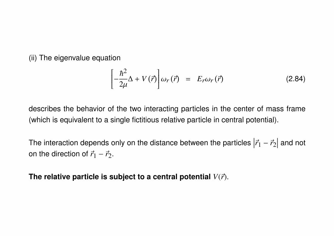
(ii) The eigenvalue equation−~22µ∆ + V

(~r)ωr

(~r)

= Erωr(~r)

(2.84)

describes the behavior of the two interacting particles in the center of mass frame(which is equivalent to a single fictitious relative particle in central potential).

The interaction depends only on the distance between the particles∣∣∣~r1 − ~r2

∣∣∣ and noton the direction of ~r1 − ~r2.

The relative particle is subject to a central potential V(~r).

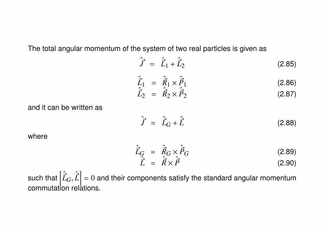
The total angular momentum of the system of two real particles is given as

~J = ~L1 + ~L2 (2.85)

~L1 = ~R1 × ~P1 (2.86)~L2 = ~R2 × ~P2 (2.87)

and it can be written as

~J = ~LG + ~L (2.88)

where

~LG = ~RG × ~PG (2.89)~L = ~R × ~P (2.90)

such that[~LG, ~L

]= 0 and their components satisfy the standard angular momentum

commutation relations.

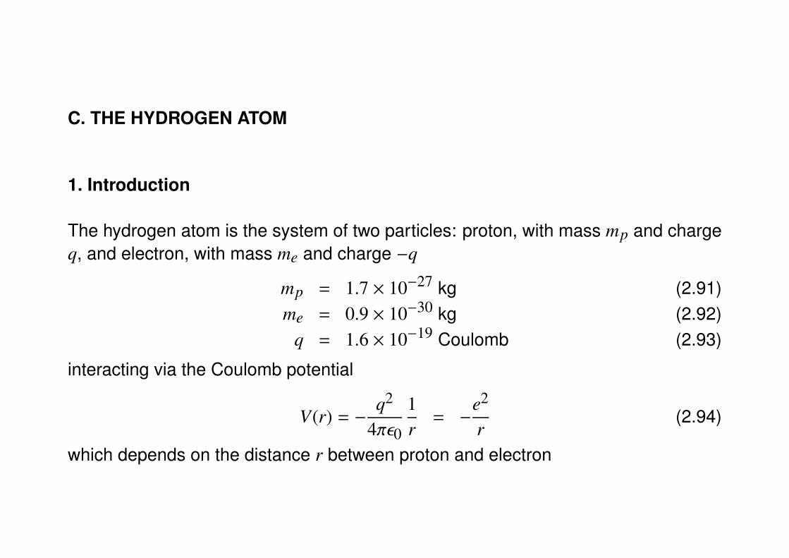
C. THE HYDROGEN ATOM

1. Introduction

The hydrogen atom is the system of two particles: proton, with mass mp and chargeq, and electron, with mass me and charge −q

mp = 1.7 × 10−27 kg (2.91)me = 0.9 × 10−30 kg (2.92)

q = 1.6 × 10−19 Coulomb (2.93)

interacting via the Coulomb potential

V(r) = −q2

4πε0

1r

= −e2

r(2.94)

which depends on the distance r between proton and electron

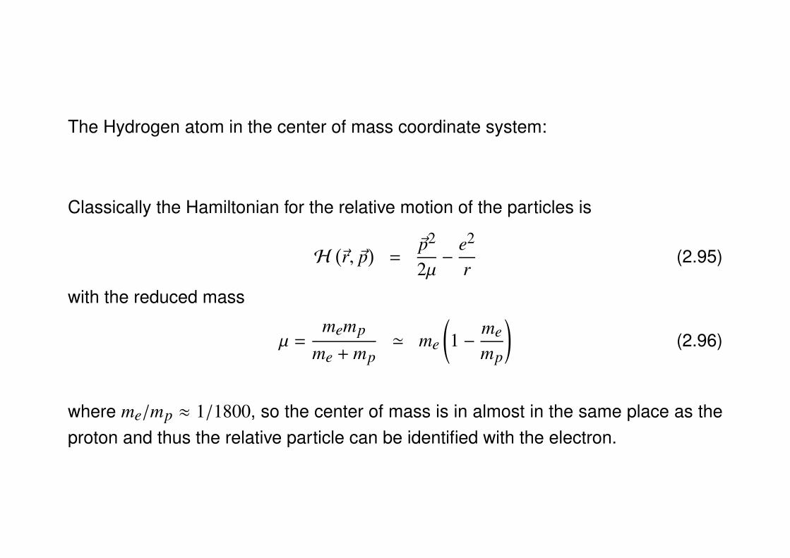
The Hydrogen atom in the center of mass coordinate system:

Classically the Hamiltonian for the relative motion of the particles is

H(~r, ~p

)=

~p2

2µ−

e2

r(2.95)

with the reduced mass

µ =memp

me + mp' me

(1 −

memp

)(2.96)

where me/mp ≈ 1/1800, so the center of mass is in almost in the same place as theproton and thus the relative particle can be identified with the electron.

2. The Bohr model

Niels Bohr postulated fixed classical orbits for motion of electron around proton

E =12µv2 −

e2

r(2.97)

The force, given as µ × acceleration of circular motion, equals to the Coulomb force

µv2

r=

e2

r2 (2.98)

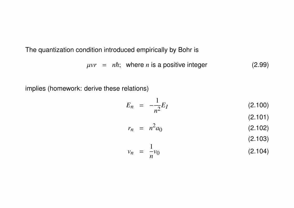
The quantization condition introduced empirically by Bohr is

µvr = n~; where n is a positive integer (2.99)

implies (homework: derive these relations)

En = −1n2EI (2.100)

(2.101)

rn = n2a0 (2.102)

(2.103)

vn =1n

v0 (2.104)

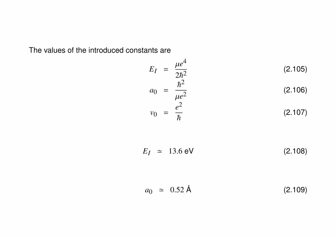
The values of the introduced constants are

EI =µe4

2~2(2.105)

a0 =~2

µe2 (2.106)

v0 =e2

~(2.107)

EI ' 13.6 eV (2.108)

a0 ' 0.52 Å (2.109)

The Bohr model yielded the correct values for the energy levels of the hydrogenatom. Moreover, it provides correct value of the ionization energy EI and the Bohrradium a0 and thus correctly characterizes atomic dimensions.

However, its classical character prevents it to be the ultimate theory of the hydrogenatom which would be free of internal inconsistencies.

Quantum theory of the hydrogen atom is free of these inconsistencies.

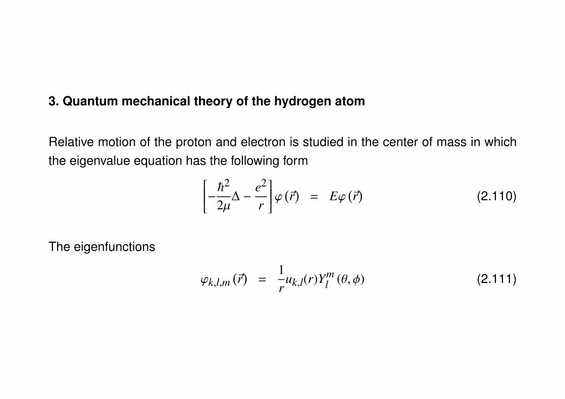
3. Quantum mechanical theory of the hydrogen atom

Relative motion of the proton and electron is studied in the center of mass in whichthe eigenvalue equation has the following form−~22µ

∆ −e2

r

ϕ (~r)

= Eϕ(~r)

(2.110)

The eigenfunctions

ϕk,l,m(~r)

=1r

uk,l(r)Yml (θ, φ) (2.111)

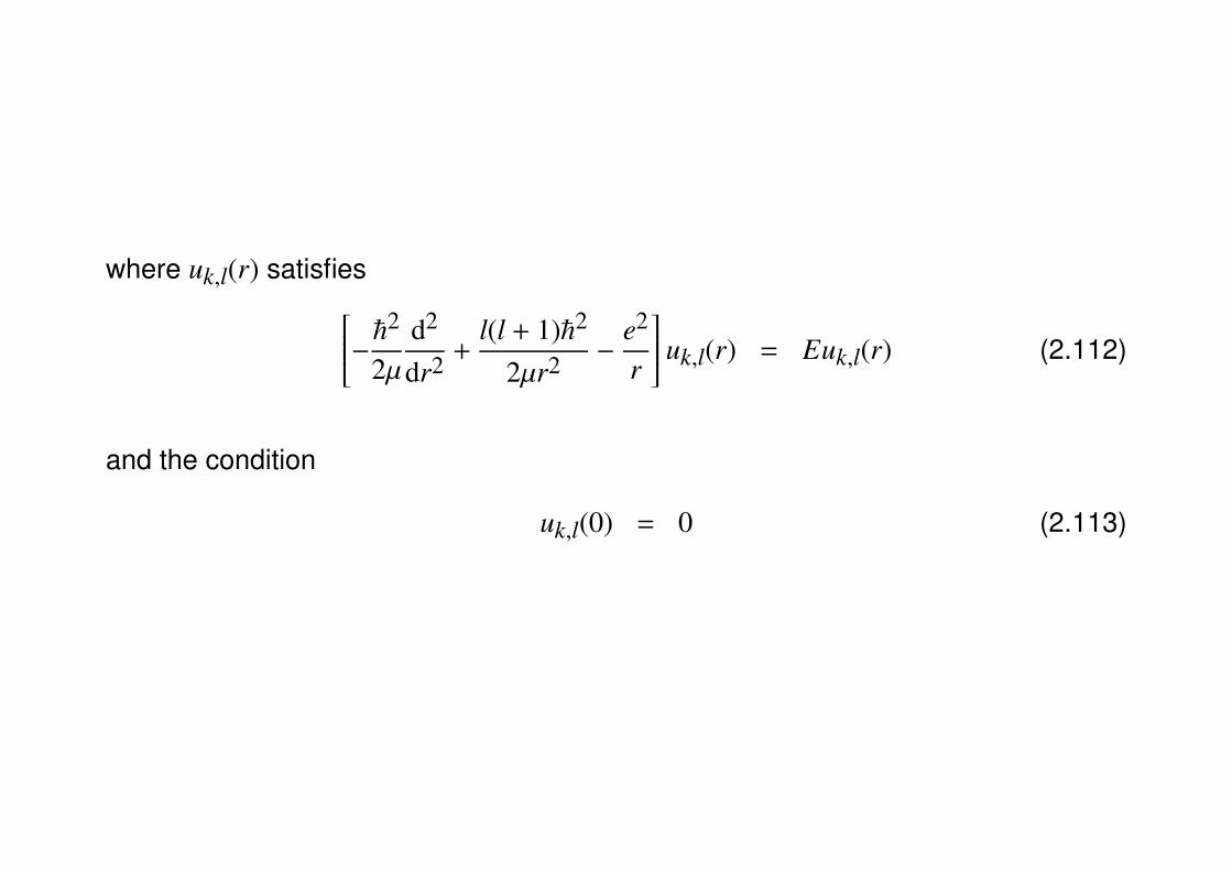
where uk,l(r) satisfies−~22µd2

dr2 +l(l + 1)~2

2µr2 −e2

r

uk,l(r) = Euk,l(r) (2.112)

and the condition

uk,l(0) = 0 (2.113)

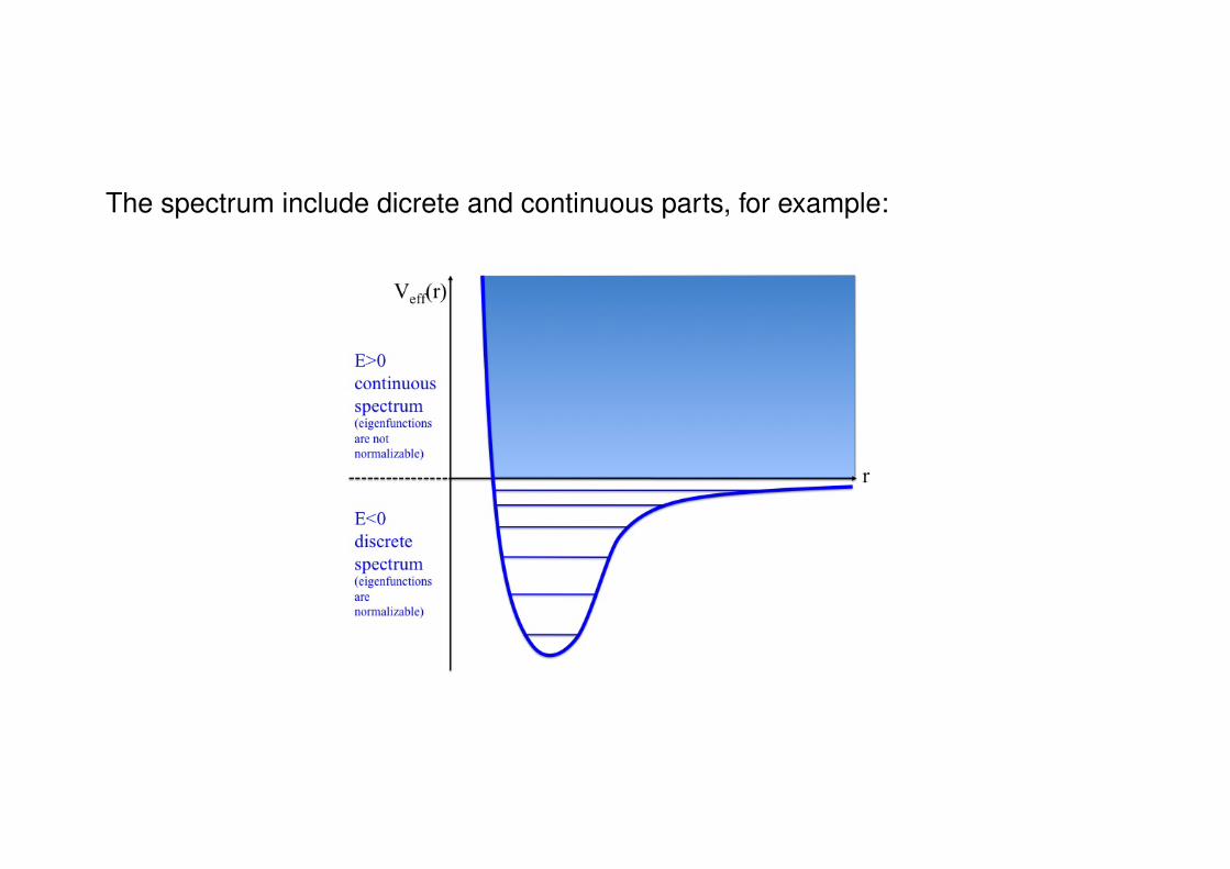
The spectrum include dicrete and continuous parts, for example:

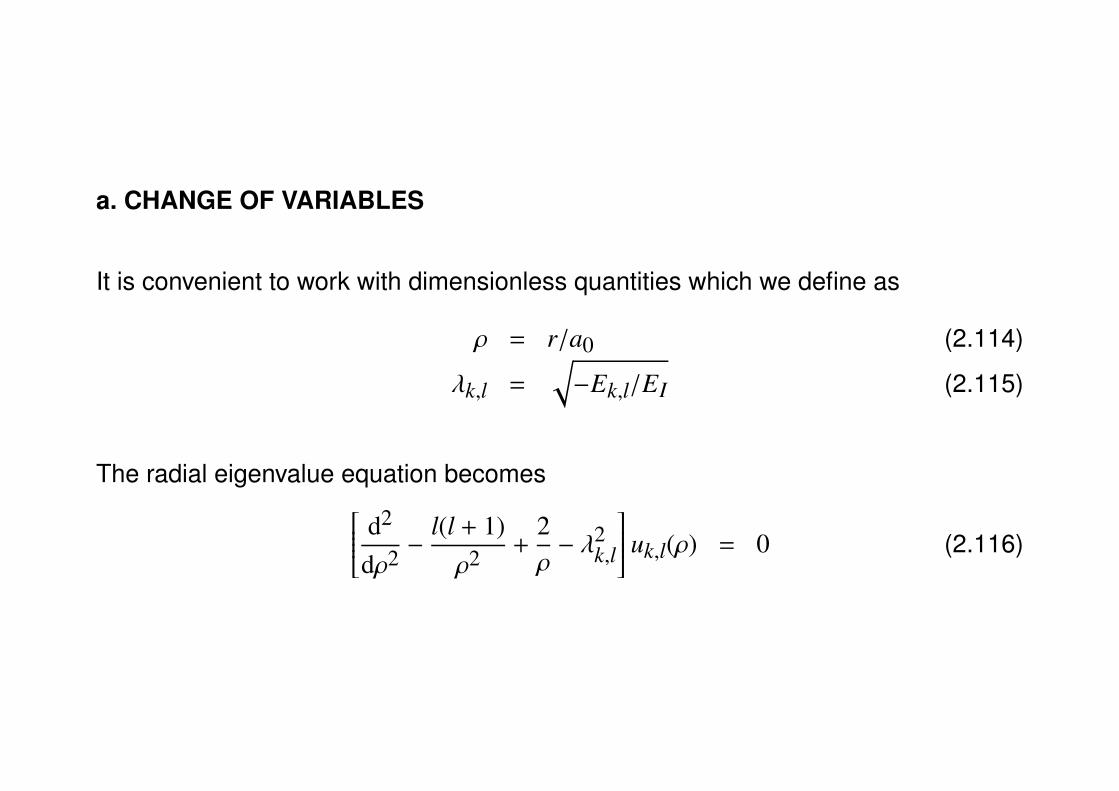
a. CHANGE OF VARIABLES

It is convenient to work with dimensionless quantities which we define as

ρ = r/a0 (2.114)

λk,l =

√−Ek,l/EI (2.115)

The radial eigenvalue equation becomes d2

dρ2 −l(l + 1)ρ2 +

2ρ− λ2

k,l

uk,l(ρ) = 0 (2.116)

b. SOLVING THE RADIAL EQUATION

We will seek the solution by expanding uk,l(ρ) in power series but first we will have alook at its asymptotic behavior.

α. Asymptotic behavior

For ρ → ∞ the terms in the eigenvalue equation above proportional to 1/ρ and 1/ρ2

are much smaller than λ2k,l, so we can neglect them obtaining d2

dρ2 − λ2k,l

uk,l(ρ) = 0 (2.117)

At this limit the solution therefore is e±ρλk,l.

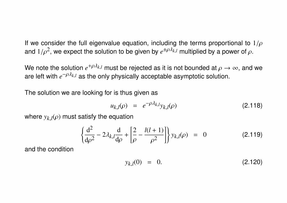
If we consider the full eigenvalue equation, including the terms proportional to 1/ρand 1/ρ2, we expect the solution to be given by e±ρλk,l multiplied by a power of ρ.

We note the solution e+ρλk,l must be rejected as it is not bounded at ρ → ∞, and weare left with e−ρλk,l as the only physically acceptable asymptotic solution.

The solution we are looking for is thus given as

uk,l(ρ) = e−ρλk,lyk,l(ρ) (2.118)

where yk,l(ρ) must satisfy the equation d2

dρ2 − 2λk,ld

dρ+

[2ρ−

l(l + 1)ρ2

] yk,l(ρ) = 0 (2.119)

and the condition

yk,l(0) = 0. (2.120)

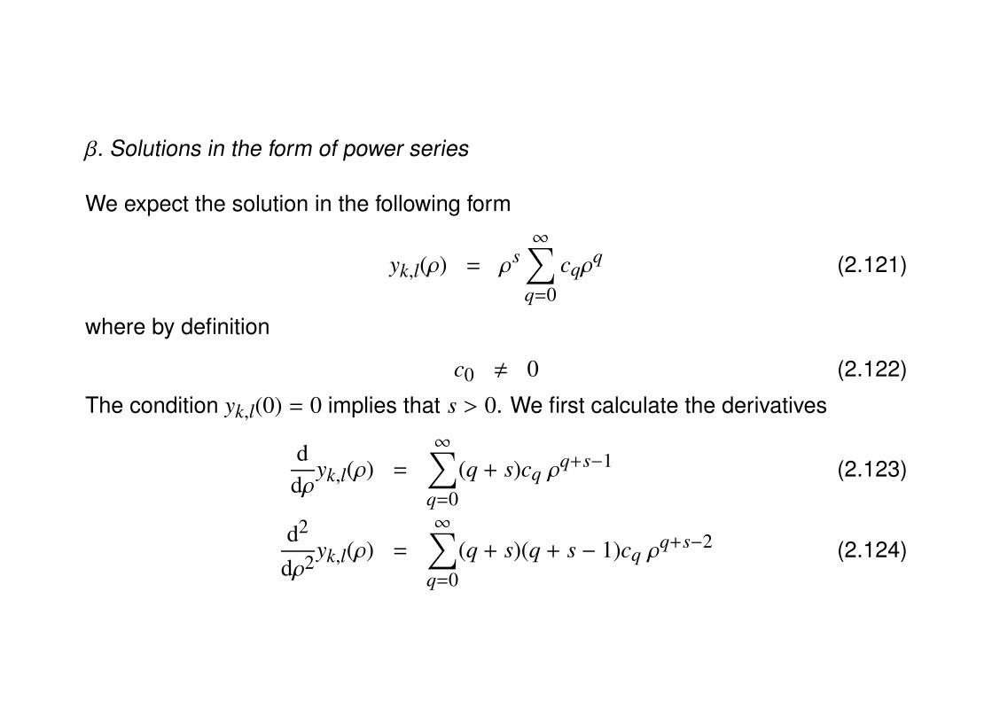
β. Solutions in the form of power series

We expect the solution in the following form

yk,l(ρ) = ρs∞∑

q=0cqρ

q (2.121)

where by definition

c0 , 0 (2.122)

The condition yk,l(0) = 0 implies that s > 0. We first calculate the derivatives

ddρ

yk,l(ρ) =

∞∑q=0

(q + s)cq ρq+s−1 (2.123)

d2

dρ2yk,l(ρ) =

∞∑q=0

(q + s)(q + s − 1)cq ρq+s−2 (2.124)

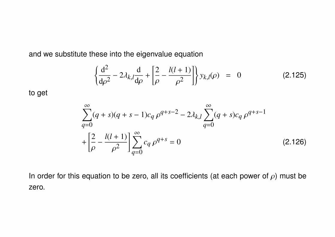
and we substitute these into the eigenvalue equation d2

dρ2 − 2λk,ld

dρ+

[2ρ−

l(l + 1)ρ2

] yk,l(ρ) = 0 (2.125)

to get

∞∑q=0

(q + s)(q + s − 1)cq ρq+s−2 − 2λk,l

∞∑q=0

(q + s)cq ρq+s−1

+

[2ρ−

l(l + 1)ρ2

] ∞∑q=0

cq ρq+s = 0 (2.126)

In order for this equation to be zero, all its coefficients (at each power of ρ) must bezero.

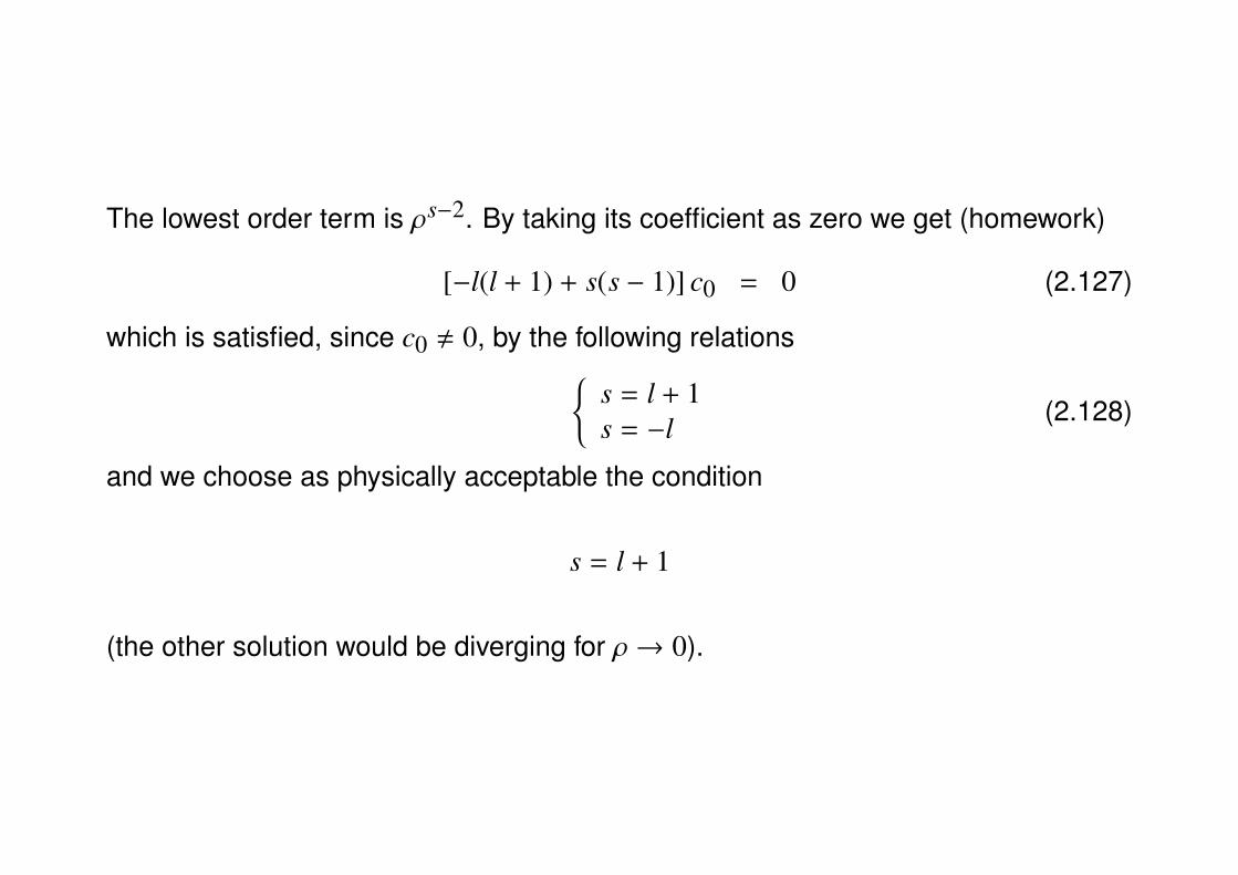
The lowest order term is ρs−2. By taking its coefficient as zero we get (homework)

[−l(l + 1) + s(s − 1)] c0 = 0 (2.127)

which is satisfied, since c0 , 0, by the following relationss = l + 1s = −l (2.128)

and we choose as physically acceptable the condition

s = l + 1

(the other solution would be diverging for ρ→ 0).

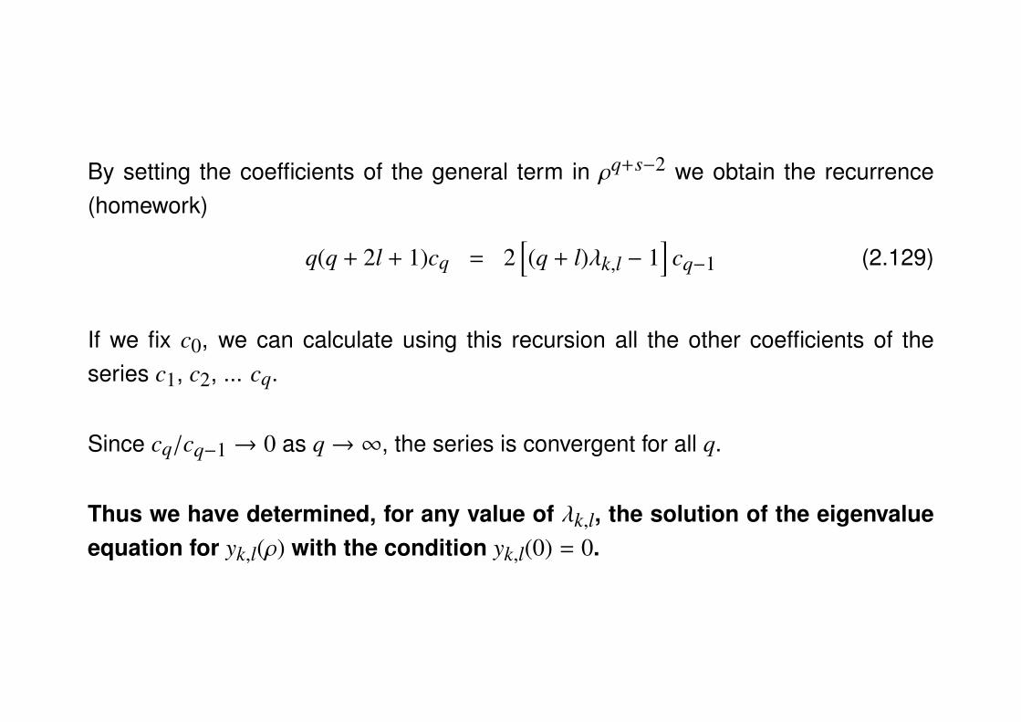
By setting the coefficients of the general term in ρq+s−2 we obtain the recurrence(homework)

q(q + 2l + 1)cq = 2[(q + l)λk,l − 1

]cq−1 (2.129)

If we fix c0, we can calculate using this recursion all the other coefficients of theseries c1, c2, ... cq.

Since cq/cq−1 → 0 as q→ ∞, the series is convergent for all q.

Thus we have determined, for any value of λk,l, the solution of the eigenvalueequation for yk,l(ρ) with the condition yk,l(0) = 0.

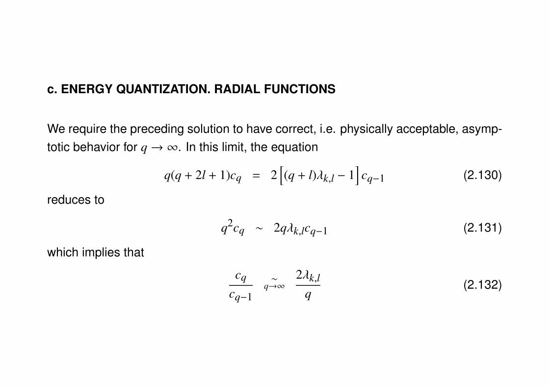
c. ENERGY QUANTIZATION. RADIAL FUNCTIONS

We require the preceding solution to have correct, i.e. physically acceptable, asymp-totic behavior for q→ ∞. In this limit, the equation

q(q + 2l + 1)cq = 2[(q + l)λk,l − 1

]cq−1 (2.130)

reduces to

q2cq ∼ 2qλk,lcq−1 (2.131)

which implies that

cq

cq−1

∼q→∞

2λk,l

q(2.132)

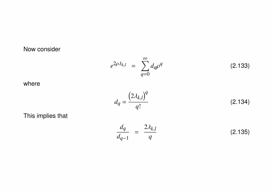
Now consider

e2ρλk,l =

∞∑q=0

dqρq (2.133)

where

dq =

(2λk,l

)q

q!(2.134)

This implies that

dq

dq−1=

2λk,l

q(2.135)

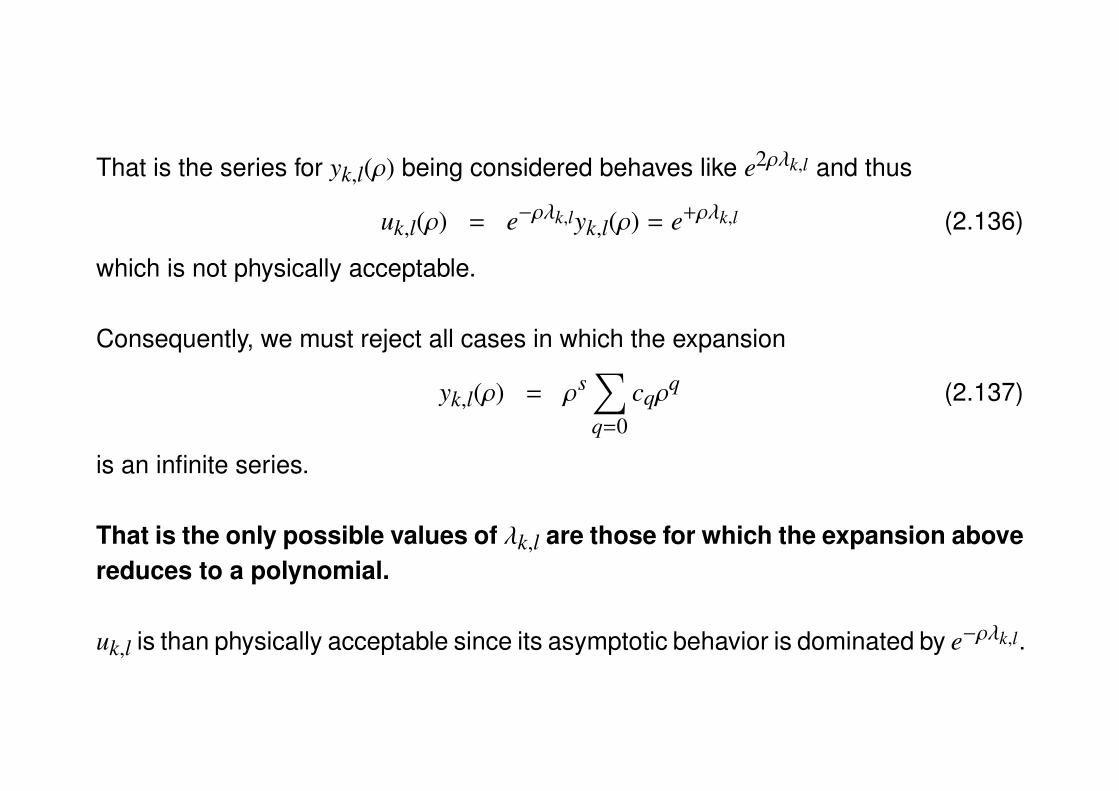
That is the series for yk,l(ρ) being considered behaves like e2ρλk,l and thus

uk,l(ρ) = e−ρλk,lyk,l(ρ) = e+ρλk,l (2.136)

which is not physically acceptable.

Consequently, we must reject all cases in which the expansion

yk,l(ρ) = ρs∑q=0

cqρq (2.137)

is an infinite series.

That is the only possible values of λk,l are those for which the expansion abovereduces to a polynomial.

uk,l is than physically acceptable since its asymptotic behavior is dominated by e−ρλk,l.

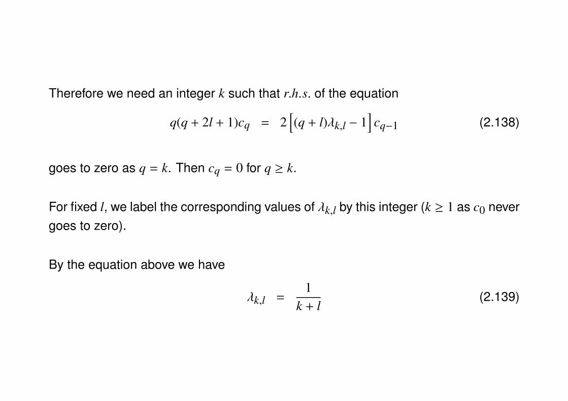
Therefore we need an integer k such that r.h.s. of the equation

q(q + 2l + 1)cq = 2[(q + l)λk,l − 1

]cq−1 (2.138)

goes to zero as q = k. Then cq = 0 for q ≥ k.

For fixed l, we label the corresponding values of λk,l by this integer (k ≥ 1 as c0 nevergoes to zero).

By the equation above we have

λk,l =1

k + l(2.139)

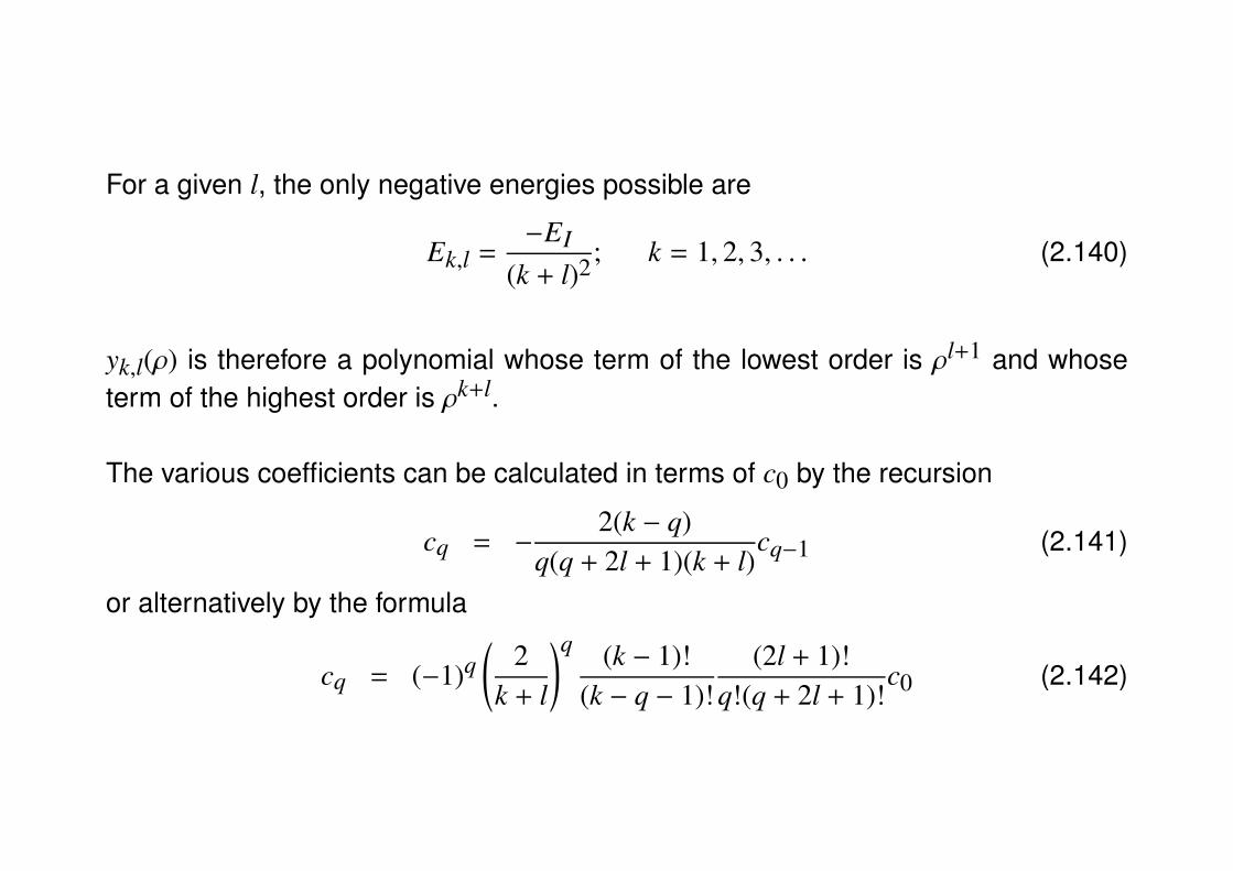
For a given l, the only negative energies possible are

Ek,l =−EI

(k + l)2 ; k = 1, 2, 3, . . . (2.140)

yk,l(ρ) is therefore a polynomial whose term of the lowest order is ρl+1 and whoseterm of the highest order is ρk+l.

The various coefficients can be calculated in terms of c0 by the recursion

cq = −2(k − q)

q(q + 2l + 1)(k + l)cq−1 (2.141)

or alternatively by the formula

cq = (−1)q(

2k + l

)q (k − 1)!(k − q − 1)!

(2l + 1)!q!(q + 2l + 1)!

c0 (2.142)

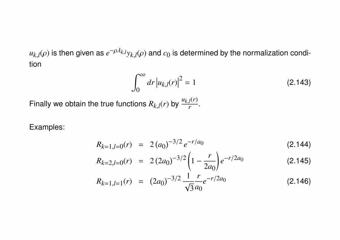
uk,l(ρ) is then given as e−ρλk,lyk,l(ρ) and c0 is determined by the normalization condi-tion ∫ ∞

0dr

∣∣∣uk,l(r)∣∣∣2 = 1 (2.143)

Finally we obtain the true functions Rk,l(r) byuk,l(r)

r .

Examples:

Rk=1,l=0(r) = 2(a0

)−3/2 e−r/a0 (2.144)

Rk=2,l=0(r) = 2(2a0

)−3/2(1 −

r2a0

)e−r/2a0 (2.145)

Rk=1,l=1(r) =(2a0

)−3/2 1√

3

ra0

e−r/2a0 (2.146)

4. Discussion of the results

a. ORDER OF MAGNITUDE OF ATOMIC PARAMETERS

The ionization energy EI and the Bohr radius a0 play important roles in giving anorder of magnitude of the energies and spatial extensions of the wavefunctions

EI =12α2µc2 (2.147)

a0 =1αoC (2.148)

where

α =e2

~c=

q2

2πε0~c'

1137

(2.149)

oC =~

µc'~

mec' 3.8 × 10−3 Å (2.150)

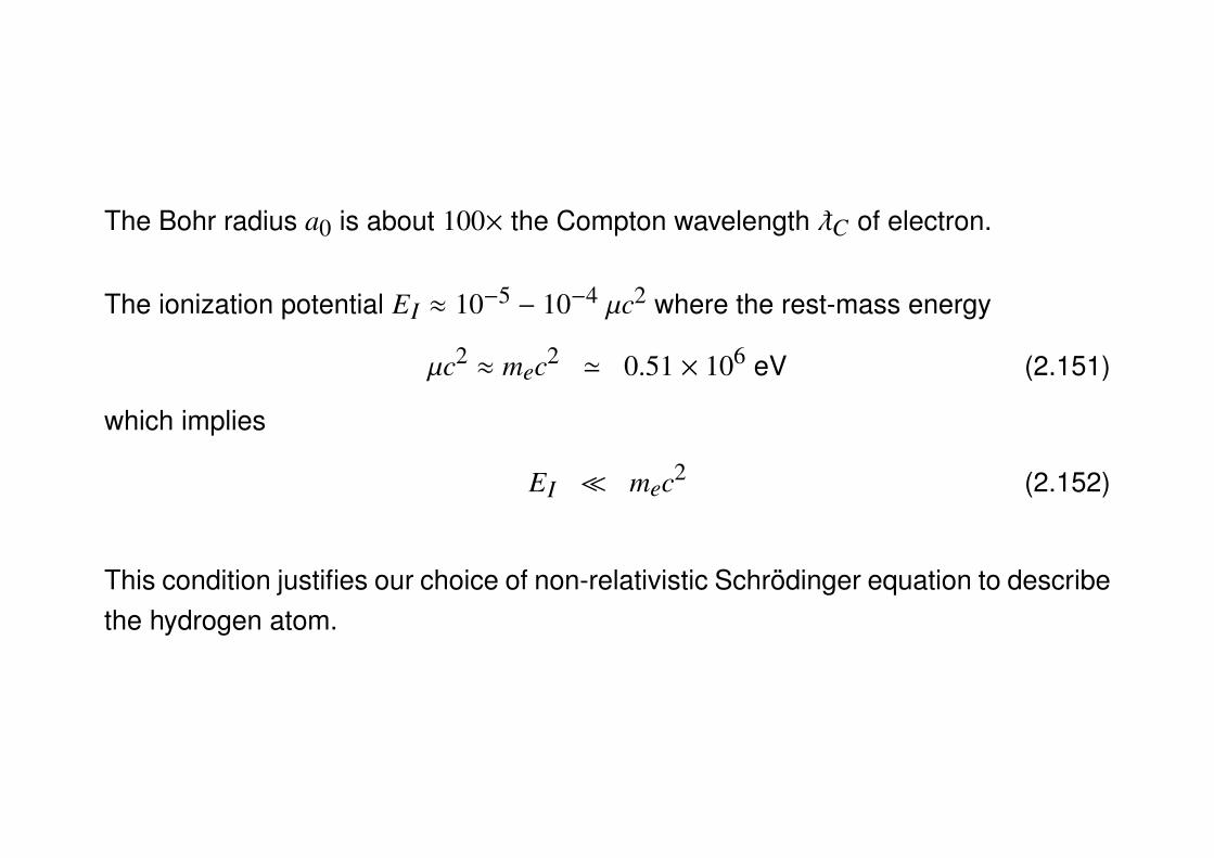
The Bohr radius a0 is about 100× the Compton wavelength oC of electron.

The ionization potential EI ≈ 10−5 − 10−4 µc2 where the rest-mass energy

µc2 ≈ mec2 ' 0.51 × 106 eV (2.151)

which implies

EI mec2 (2.152)

This condition justifies our choice of non-relativistic Schrodinger equation to describethe hydrogen atom.

b. ENERGY LEVELS

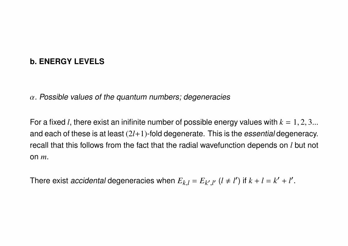
α. Possible values of the quantum numbers; degeneracies

For a fixed l, there exist an inifinite number of possible energy values with k = 1, 2, 3...and each of these is at least (2l+1)-fold degenerate. This is the essential degeneracy.recall that this follows from the fact that the radial wavefunction depends on l but noton m.

There exist accidental degeneracies when Ek,l = Ek′,l′ (l , l′) if k + l = k′ + l′.

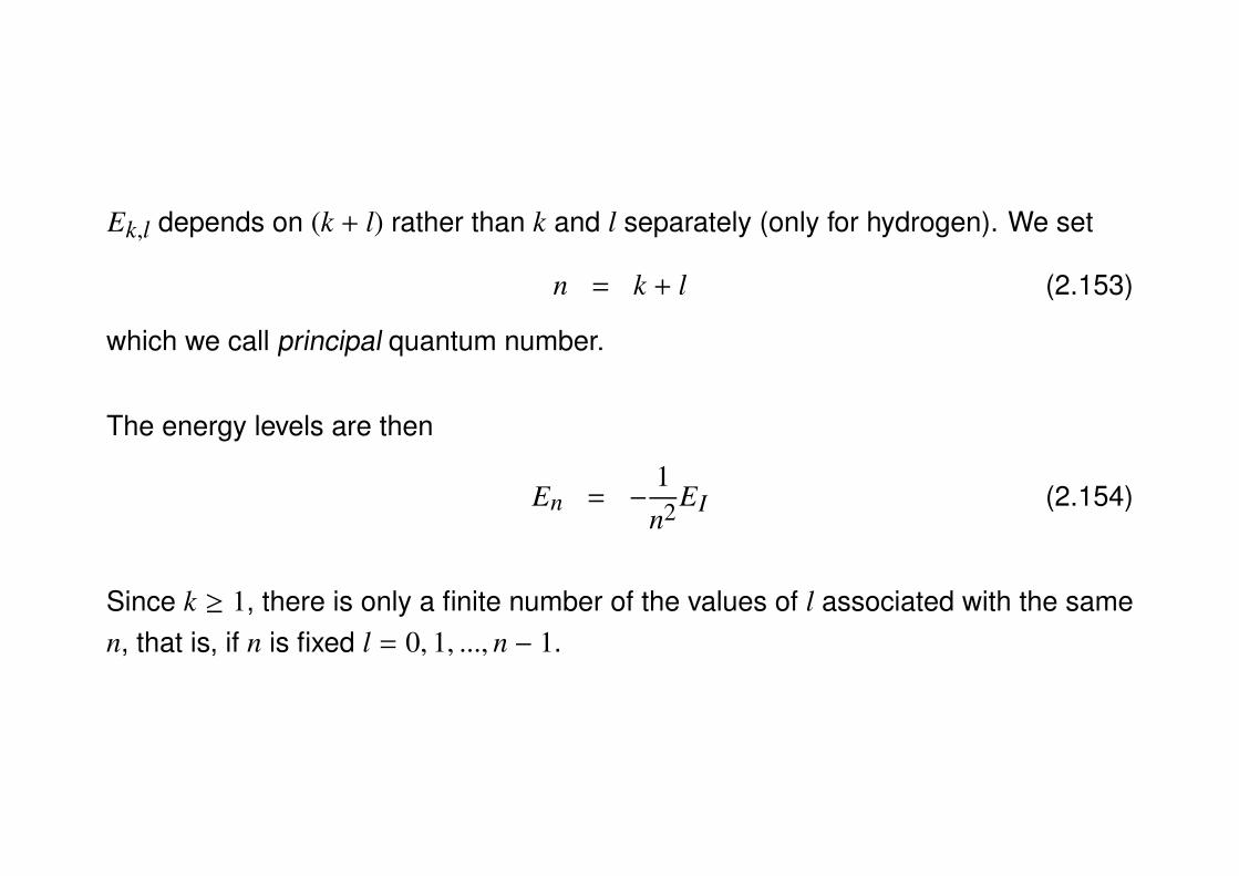
Ek,l depends on (k + l) rather than k and l separately (only for hydrogen). We set

n = k + l (2.153)

which we call principal quantum number.

The energy levels are then

En = −1n2EI (2.154)

Since k ≥ 1, there is only a finite number of the values of l associated with the samen, that is, if n is fixed l = 0, 1, ..., n − 1.

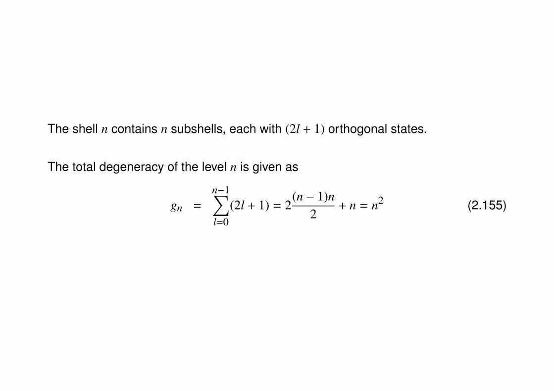
The shell n contains n subshells, each with (2l + 1) orthogonal states.

The total degeneracy of the level n is given as

gn =

n−1∑l=0

(2l + 1) = 2(n − 1)n

2+ n = n2 (2.155)

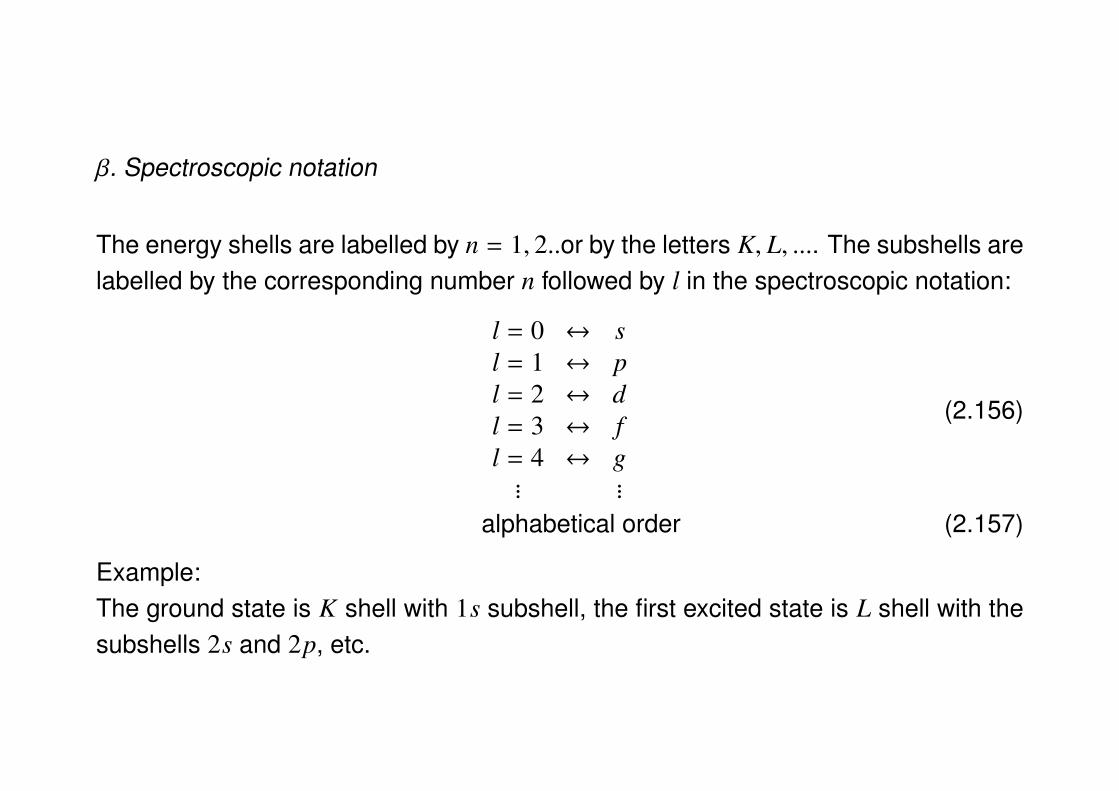
β. Spectroscopic notation

The energy shells are labelled by n = 1, 2..or by the letters K, L, .... The subshells arelabelled by the corresponding number n followed by l in the spectroscopic notation:

l = 0 ↔ sl = 1 ↔ pl = 2 ↔ dl = 3 ↔ fl = 4 ↔ g... ...

(2.156)

alphabetical order (2.157)

Example:The ground state is K shell with 1s subshell, the first excited state is L shell with thesubshells 2s and 2p, etc.

The hydrogen atom energy levels

c. WAVE FUNCTIONS

Wavefunctions are labeled by the quantum numbers n, l, and m which uniquely char-acterize the eigenfunctions φn,l,m(~r) of the C.S.C.O. H, L2, and Lz.

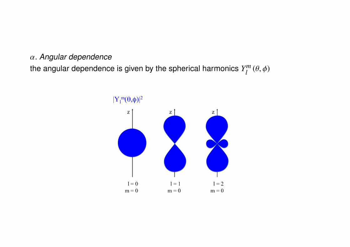
α. Angular dependencethe angular dependence is given by the spherical harmonics Ym

l (θ, φ)

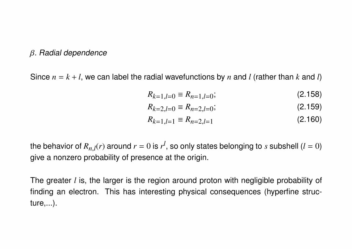
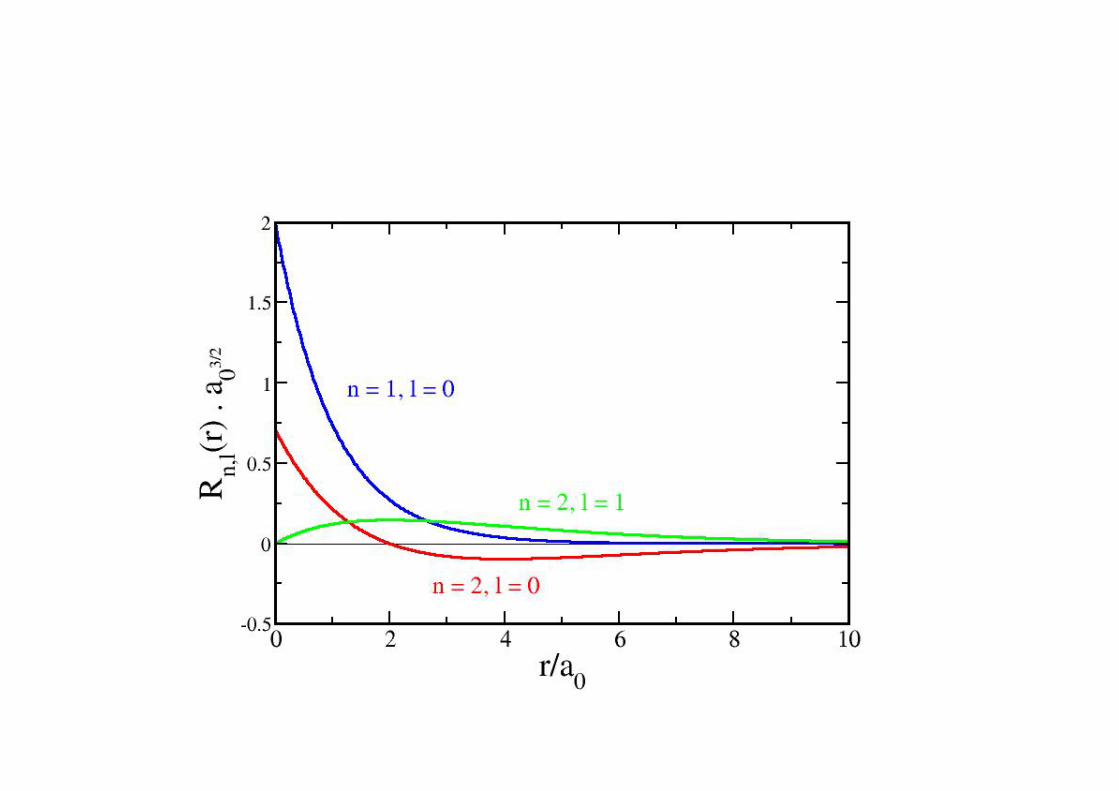
β. Radial dependence

Since n = k + l, we can label the radial wavefunctions by n and l (rather than k and l)

Rk=1,l=0 ≡ Rn=1,l=0; (2.158)

Rk=2,l=0 ≡ Rn=2,l=0; (2.159)

Rk=1,l=1 ≡ Rn=2,l=1 (2.160)

the behavior of Rn,l(r) around r = 0 is rl, so only states belonging to s subshell (l = 0)give a nonzero probability of presence at the origin.

The greater l is, the larger is the region around proton with negligible probability offinding an electron. This has interesting physical consequences (hyperfine struc-ture,...).

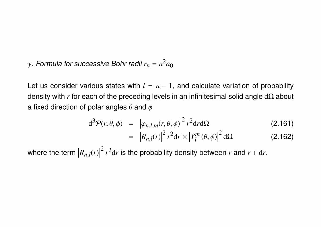
γ. Formula for successive Bohr radii rn = n2a0

Let us consider various states with l = n − 1, and calculate variation of probabilitydensity with r for each of the preceding levels in an infinitesimal solid angle dΩ abouta fixed direction of polar angles θ and φ

d3P(r, θ, φ) =∣∣∣ϕn,l,m(r, θ, φ)

∣∣∣2 r2drdΩ (2.161)

=∣∣∣Rn,l(r)

∣∣∣2 r2dr ×∣∣∣Ym

l (θ, φ)∣∣∣2 dΩ (2.162)

where the term∣∣∣Rn,l(r)

∣∣∣2 r2dr is the probability density between r and r + dr.

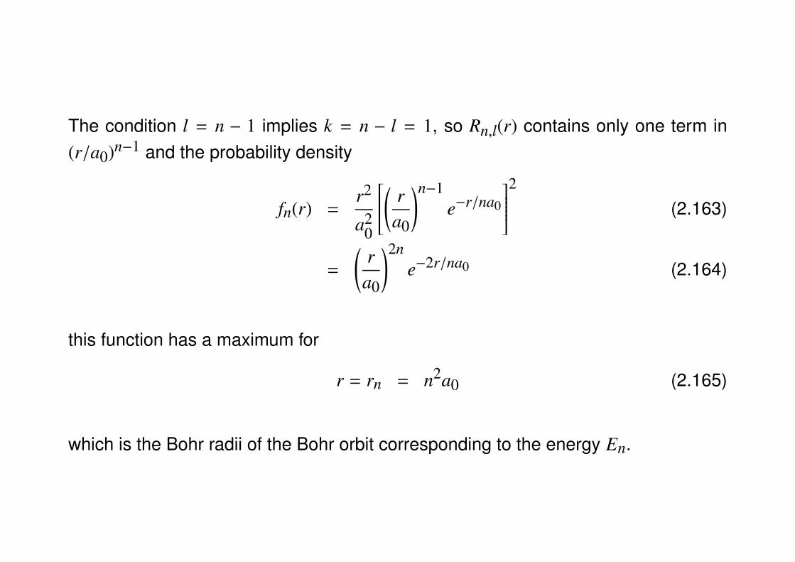
The condition l = n − 1 implies k = n − l = 1, so Rn,l(r) contains only one term in(r/a0)n−1 and the probability density

fn(r) =r2

a20

( ra0

)n−1e−r/na0

2

(2.163)

=

(r

a0

)2ne−2r/na0 (2.164)

this function has a maximum for

r = rn = n2a0 (2.165)

which is the Bohr radii of the Bohr orbit corresponding to the energy En.

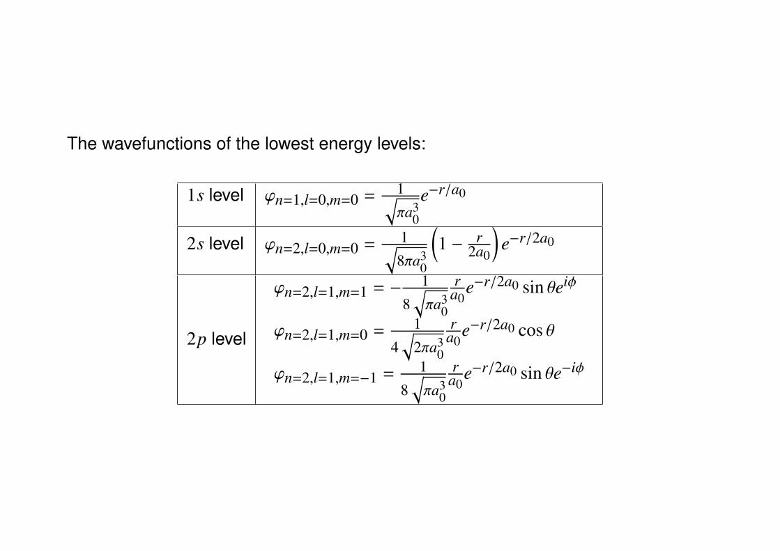
The wavefunctions of the lowest energy levels:

1s level ϕn=1,l=0,m=0 = 1√πa3

0

e−r/a0

2s level ϕn=2,l=0,m=0 = 1√8πa3

0

(1 − r

2a0

)e−r/2a0

2p level

ϕn=2,l=1,m=1 = − 1

8√πa3

0

ra0

e−r/2a0 sin θeiφ

ϕn=2,l=1,m=0 = 1

4√

2πa30

ra0

e−r/2a0 cos θ

ϕn=2,l=1,m=−1 = 1

8√πa3

0

ra0

e−r/2a0 sin θe−iφ

THE ISOTROPIC THREE-DIMENSIONAL HARMONIC OSCILLATOR(Complement BVII)

Our objectives are:

1. Solving the radial equation

2. Finding energy levels and stationary wave functions

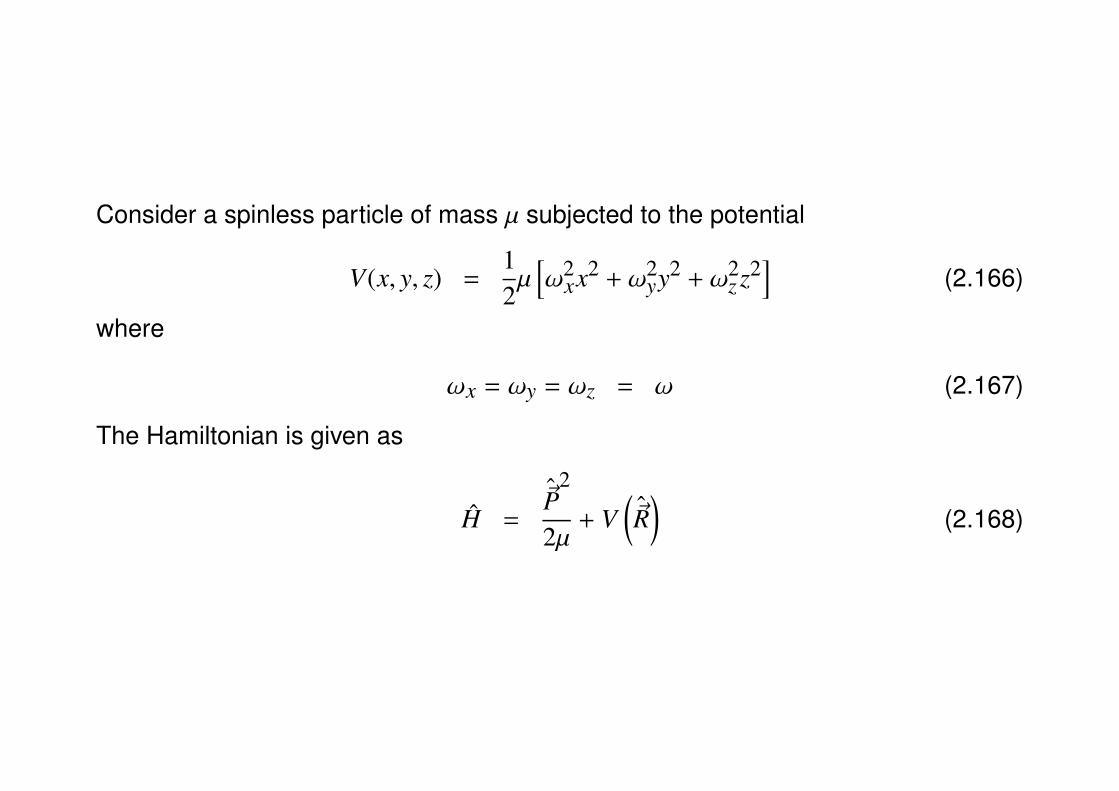
Consider a spinless particle of mass µ subjected to the potential

V(x, y, z) =12µ[ω2

xx2 + ω2yy2 + ω2

z z2]

(2.166)

where

ωx = ωy = ωz = ω (2.167)

The Hamiltonian is given as

H =~P

2

2µ+ V

(~R)

(2.168)

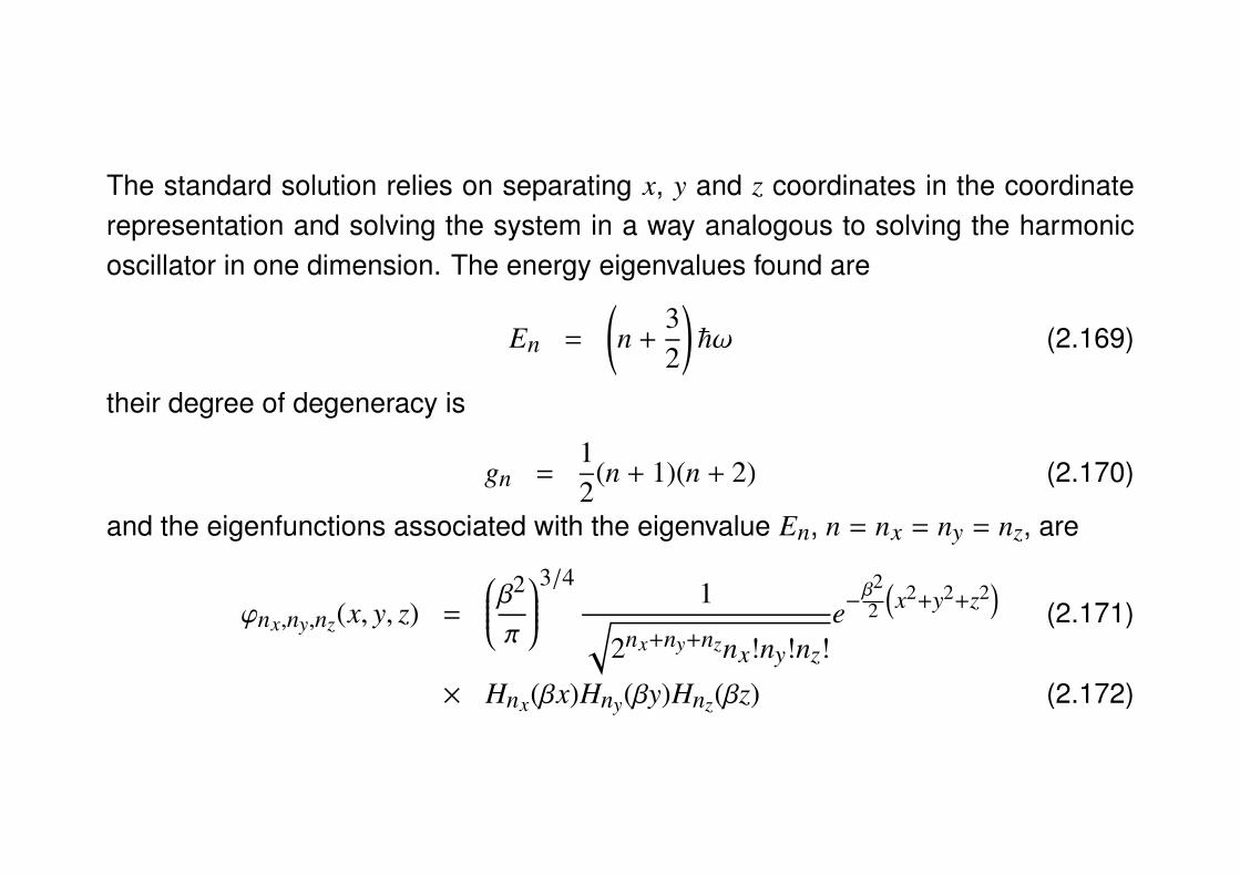
The standard solution relies on separating x, y and z coordinates in the coordinaterepresentation and solving the system in a way analogous to solving the harmonicoscillator in one dimension. The energy eigenvalues found are

En =

(n +

32

)~ω (2.169)

their degree of degeneracy is

gn =12

(n + 1)(n + 2) (2.170)

and the eigenfunctions associated with the eigenvalue En, n = nx = ny = nz, are

ϕnx,ny,nz(x, y, z) =

β2

π

3/4 1√2nx+ny+nznx!ny!nz!

e−β22

(x2+y2+z2

)(2.171)

× Hnx(βx)Hny(βy)Hnz(βz) (2.172)

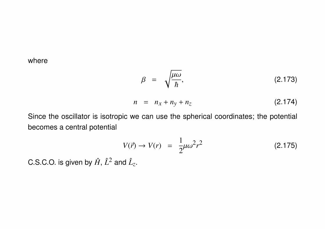
where

β =

√µω

~, (2.173)

n = nx + ny + nz (2.174)

Since the oscillator is isotropic we can use the spherical coordinates; the potentialbecomes a central potential

V(~r)→ V(r) =12µω2r2 (2.175)

C.S.C.O. is given by H, L2 and Lz.

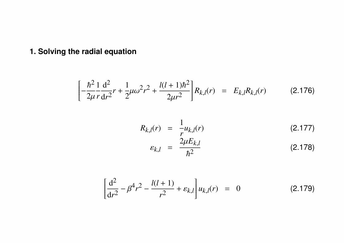
1. Solving the radial equation

−~22µ1r

d2

dr2r +12µω2r2 +

l(l + 1)~2

2µr2

Rk,l(r) = Ek,lRk,l(r) (2.176)

Rk,l(r) =1r

uk,l(r) (2.177)

εk,l =2µEk,l

~2(2.178)

d2

dr2 − β4r2 −

l(l + 1)r2 + εk,l

uk,l(r) = 0 (2.179)

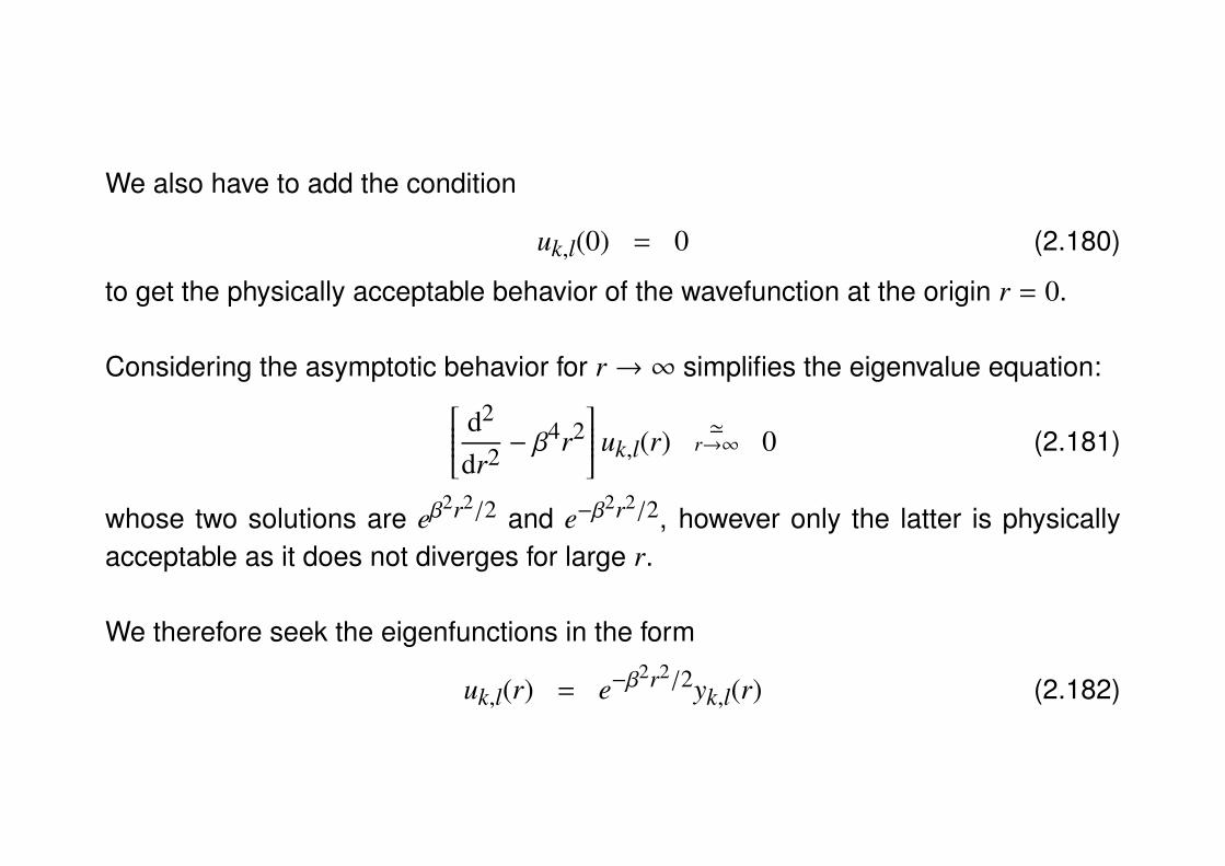
We also have to add the condition

uk,l(0) = 0 (2.180)

to get the physically acceptable behavior of the wavefunction at the origin r = 0.

Considering the asymptotic behavior for r → ∞ simplifies the eigenvalue equation: d2

dr2 − β4r2

uk,l(r) 'r→∞ 0 (2.181)

whose two solutions are eβ2r2/2 and e−β

2r2/2, however only the latter is physicallyacceptable as it does not diverges for large r.

We therefore seek the eigenfunctions in the form

uk,l(r) = e−β2r2/2yk,l(r) (2.182)

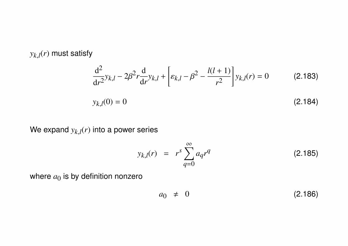
yk,l(r) must satisfy

d2

dr2yk,l − 2β2rddr

yk,l +

[εk,l − β

2 −l(l + 1)

r2

]yk,l(r) = 0 (2.183)

yk,l(0) = 0 (2.184)

We expand yk,l(r) into a power series

yk,l(r) = rs∞∑

q=0aqrq (2.185)

where a0 is by definition nonzero

a0 , 0 (2.186)

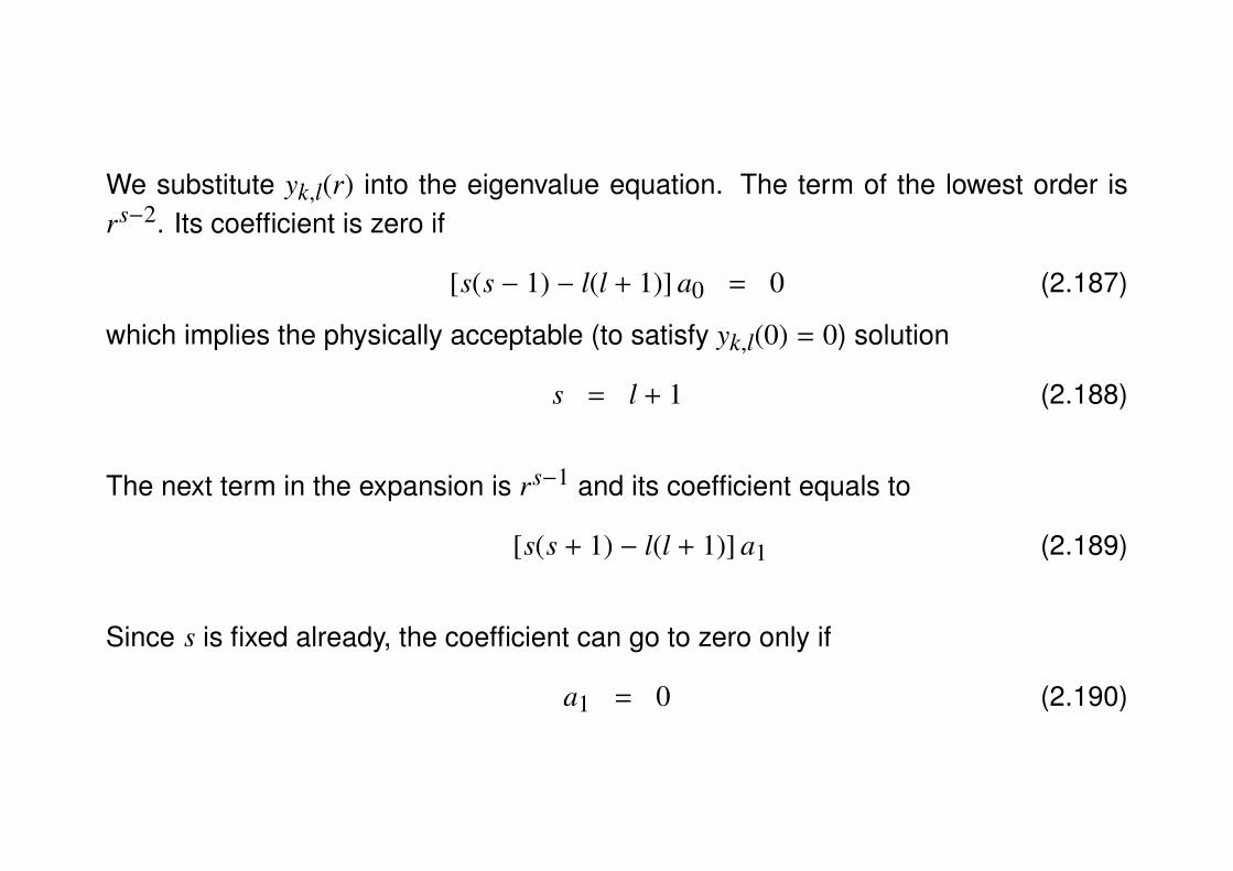
We substitute yk,l(r) into the eigenvalue equation. The term of the lowest order isrs−2. Its coefficient is zero if

[s(s − 1) − l(l + 1)] a0 = 0 (2.187)

which implies the physically acceptable (to satisfy yk,l(0) = 0) solution

s = l + 1 (2.188)

The next term in the expansion is rs−1 and its coefficient equals to

[s(s + 1) − l(l + 1)] a1 (2.189)

Since s is fixed already, the coefficient can go to zero only if

a1 = 0 (2.190)

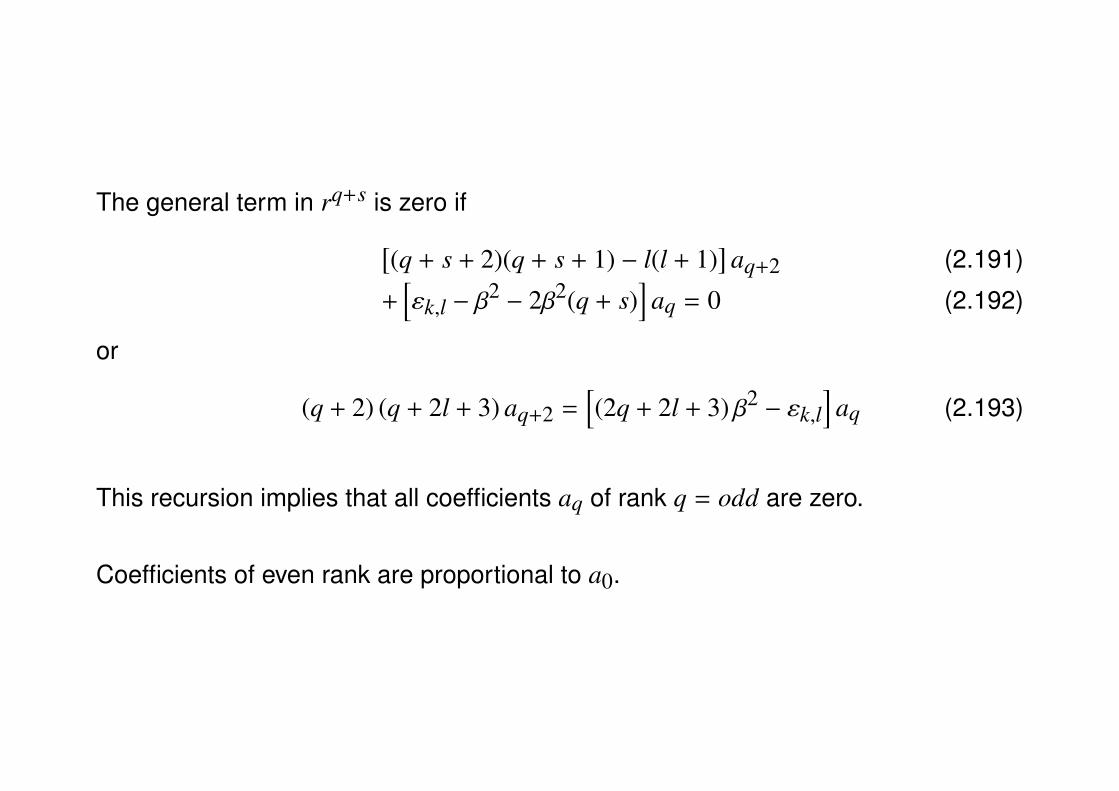
The general term in rq+s is zero if[(q + s + 2)(q + s + 1) − l(l + 1)

]aq+2 (2.191)

+[εk,l − β

2 − 2β2(q + s)]

aq = 0 (2.192)

or

(q + 2) (q + 2l + 3) aq+2 =[(2q + 2l + 3) β2 − εk,l

]aq (2.193)

This recursion implies that all coefficients aq of rank q = odd are zero.

Coefficients of even rank are proportional to a0.

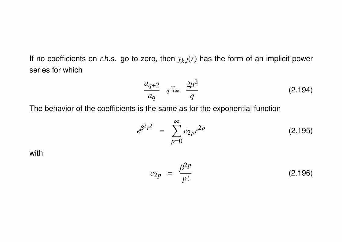
If no coefficients on r.h.s. go to zero, then yk,l(r) has the form of an implicit powerseries for which

aq+2

aq

∼q→∞

2β2

q(2.194)

The behavior of the coefficients is the same as for the exponential function

eβ2r2

=

∞∑p=0

c2pr2p (2.195)

with

c2p =β2p

p!(2.196)

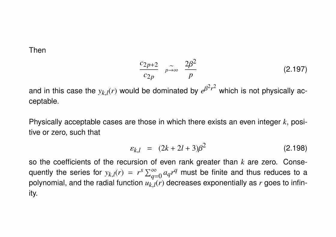
Then

c2p+2

c2p

∼p→∞

2β2

p(2.197)

and in this case the yk,l(r) would be dominated by eβ2r2

which is not physically ac-ceptable.

Physically acceptable cases are those in which there exists an even integer k, posi-tive or zero, such that

εk,l = (2k + 2l + 3)β2 (2.198)

so the coefficients of the recursion of even rank greater than k are zero. Conse-quently the series for yk,l(r) = rs ∑∞

q=0 aqrq must be finite and thus reduces to apolynomial, and the radial function uk,l(r) decreases exponentially as r goes to infin-ity.

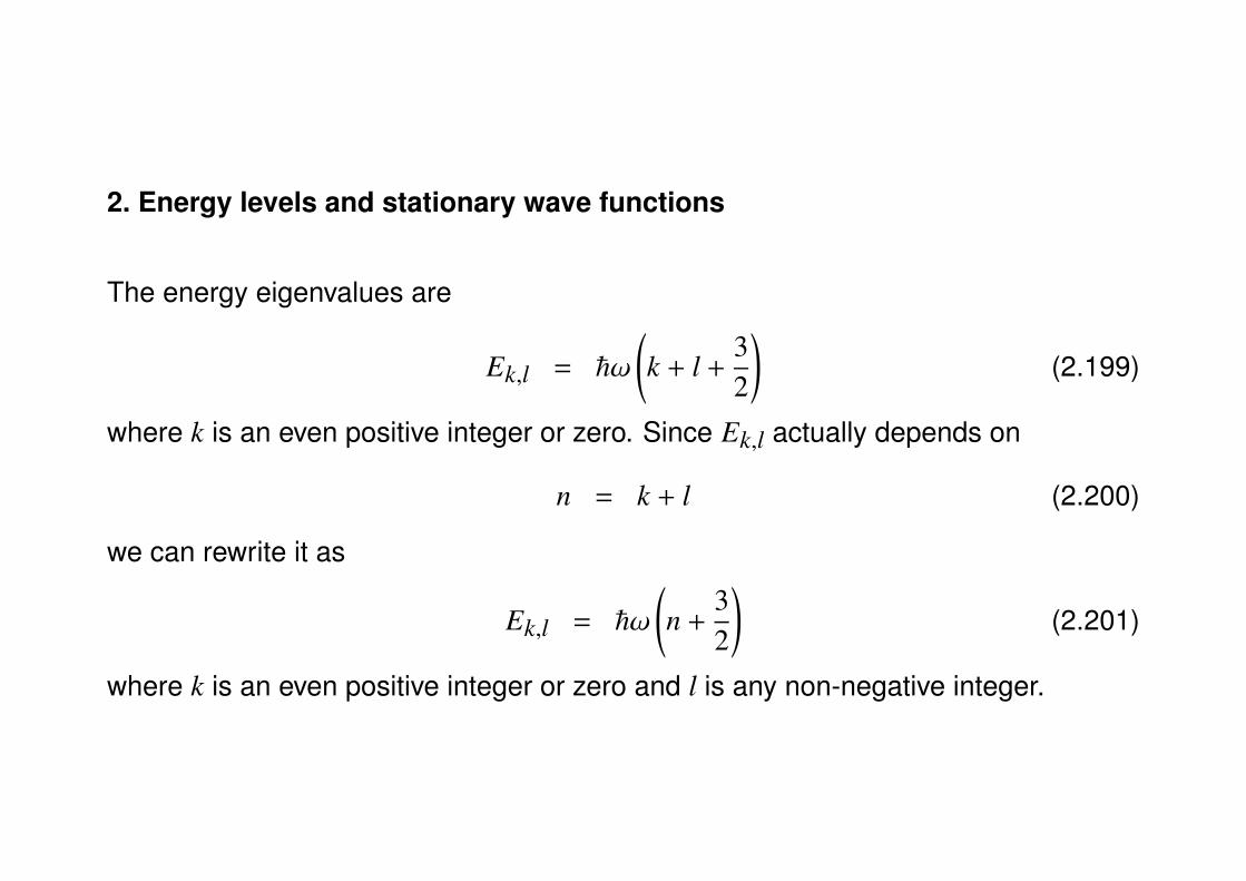
2. Energy levels and stationary wave functions

The energy eigenvalues are

Ek,l = ~ω

(k + l +

32

)(2.199)

where k is an even positive integer or zero. Since Ek,l actually depends on

n = k + l (2.200)

we can rewrite it as

Ek,l = ~ω

(n +

32

)(2.201)

where k is an even positive integer or zero and l is any non-negative integer.

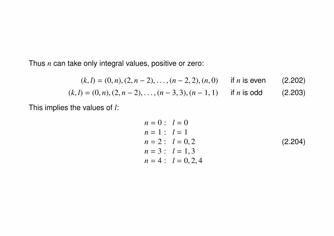
Thus n can take only integral values, positive or zero:

(k, l) = (0, n), (2, n − 2), . . . , (n − 2, 2), (n, 0) if n is even (2.202)

(k, l) = (0, n), (2, n − 2), . . . , (n − 3, 3), (n − 1, 1) if n is odd (2.203)

This implies the values of l:

n = 0 : l = 0n = 1 : l = 1n = 2 : l = 0, 2n = 3 : l = 1, 3n = 4 : l = 0, 2, 4

(2.204)

En = (n + 32)~ω = 3

2~ω,52~ω,

72~ω,

92~ω,

112 ~ω, ...

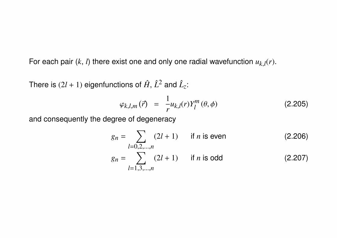
For each pair (k, l) there exist one and only one radial wavefunction uk,l(r).

There is (2l + 1) eigenfunctions of H, L2 and Lz:

ϕk,l,m(~r)

=1r

uk,l(r)Yml (θ, φ) (2.205)

and consequently the degree of degeneracy

gn =∑

l=0,2,...,n(2l + 1) if n is even (2.206)

gn =∑

l=1,3,...,n(2l + 1) if n is odd (2.207)

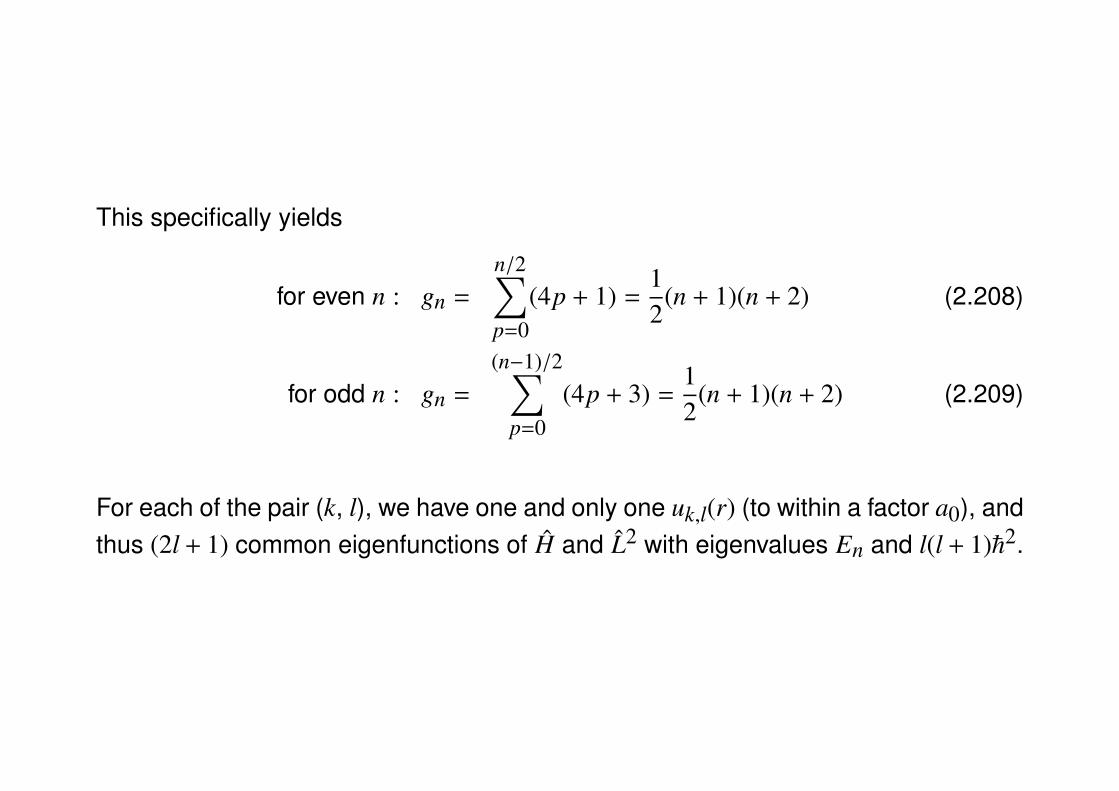
This specifically yields

for even n : gn =

n/2∑p=0

(4p + 1) =12

(n + 1)(n + 2) (2.208)

for odd n : gn =

(n−1)/2∑p=0

(4p + 3) =12

(n + 1)(n + 2) (2.209)

For each of the pair (k, l), we have one and only one uk,l(r) (to within a factor a0), andthus (2l + 1) common eigenfunctions of H and L2 with eigenvalues En and l(l + 1)~2.

Example: wavefunctions for the three lowest energy levels

(i) E0 = 32~ω

k = l = 0 (2.210)

y0,0(r) reduces to a0r where a0 is determined by normalization

ϕ0,0,0(~r)

=

β2

π

3/4

e−β2r2/2 (2.211)

The ground state is non-degenerate.

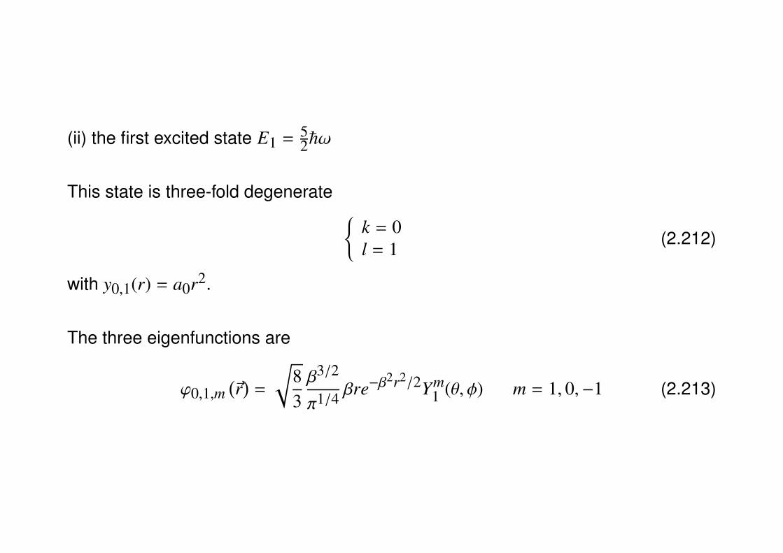
(ii) the first excited state E1 = 52~ω

This state is three-fold degenerate k = 0l = 1 (2.212)

with y0,1(r) = a0r2.

The three eigenfunctions are

ϕ0,1,m(~r)

=

√83β3/2

π1/4 βre−β2r2/2Ym

1 (θ, φ) m = 1, 0,−1 (2.213)

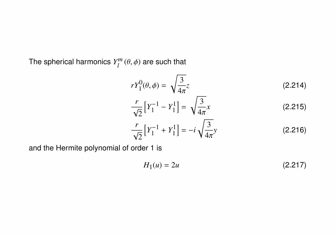
The spherical harmonics Yml (θ, φ) are such that

rY01 (θ, φ) =

√3

4πz (2.214)

r√

2

[Y−1

1 − Y11

]=

√3

4πx (2.215)

r√

2

[Y−1

1 + Y11

]= −i

√3

4πy (2.216)

and the Hermite polynomial of order 1 is

H1(u) = 2u (2.217)

so that the functions ϕ0,1,m are related to the functions ϕnx,ny,nz of the basis given bythe Hermite polynomials (Eq. (2.172)) by the equations

ϕnx=0,ny=0,nz=1 = ϕk=0,l=1,m=0 (2.218)

ϕnx=1,ny=0,nz=0 =1√

2

[ϕk=0,l=1,m=−1 − ϕk=0,l=1,m=1

](2.219)

ϕnx=0,ny=1,nz=0 =i√

2

[ϕk=0,l=1,m=−1 + ϕk=0,l=1,m=1

](2.220)

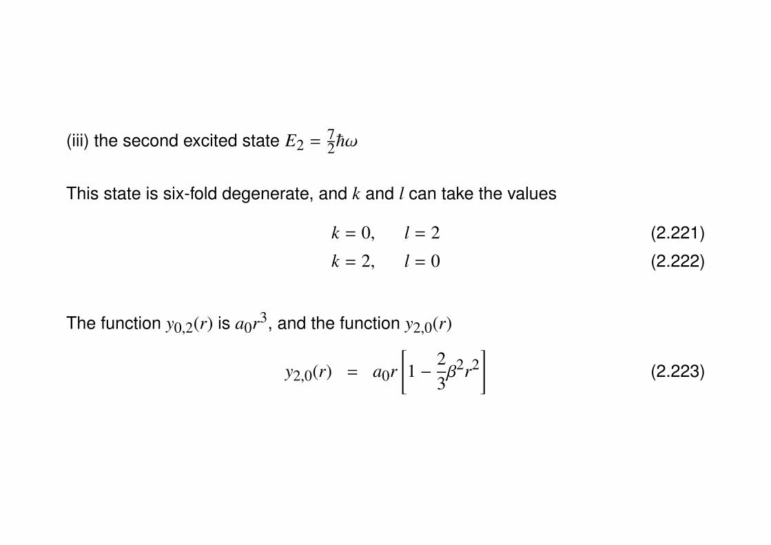
(iii) the second excited state E2 = 72~ω

This state is six-fold degenerate, and k and l can take the values

k = 0, l = 2 (2.221)

k = 2, l = 0 (2.222)

The function y0,2(r) is a0r3, and the function y2,0(r)

y2,0(r) = a0r[1 −

23β2r2

](2.223)

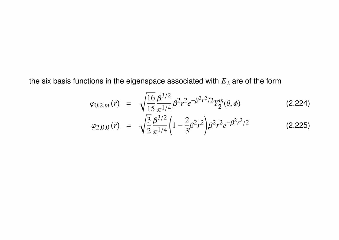
the six basis functions in the eigenspace associated with E2 are of the form

ϕ0,2,m(~r)

=

√1615

β3/2

π1/4 β2r2e−β

2r2/2Ym2 (θ, φ) (2.224)

ϕ2,0,0(~r)

=

√32β3/2

π1/4

(1 −

23β2r2

)β2r2e−β

2r2/2 (2.225)

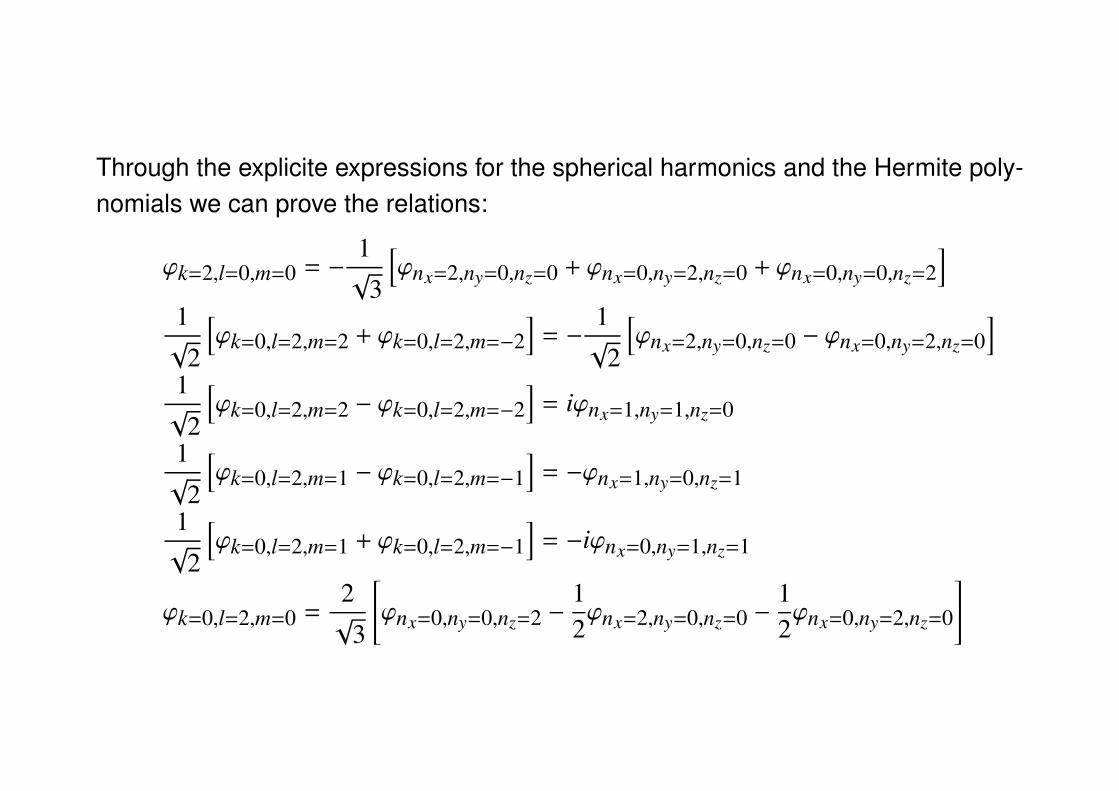
Through the explicite expressions for the spherical harmonics and the Hermite poly-nomials we can prove the relations:

ϕk=2,l=0,m=0 = −1√

3

[ϕnx=2,ny=0,nz=0 + ϕnx=0,ny=2,nz=0 + ϕnx=0,ny=0,nz=2

]1√

2

[ϕk=0,l=2,m=2 + ϕk=0,l=2,m=−2

]= −

1√

2

[ϕnx=2,ny=0,nz=0 − ϕnx=0,ny=2,nz=0

]1√

2

[ϕk=0,l=2,m=2 − ϕk=0,l=2,m=−2

]= iϕnx=1,ny=1,nz=0

1√

2

[ϕk=0,l=2,m=1 − ϕk=0,l=2,m=−1

]= −ϕnx=1,ny=0,nz=1

1√

2

[ϕk=0,l=2,m=1 + ϕk=0,l=2,m=−1

]= −iϕnx=0,ny=1,nz=1

ϕk=0,l=2,m=0 =2√

3

[ϕnx=0,ny=0,nz=2 −

12ϕnx=2,ny=0,nz=0 −

12ϕnx=0,ny=2,nz=0

]