Chapter 2 Nonlinear Finite Element Formulation for The ...Postbuckling Analysis of Stiffened...
38
Chapter 2: Nonlinear Finite Element Formulation 18 Chapter 2 Nonlinear Finite Element Formulation for The Postbuckling Analysis of Stiffened Composite Panels with Imperfections Those concepts behind the Finite Element method which are useful in applying the basic theory to the postbuckling analysis of stiffened composite panels will be briefly outlined in this chapter. However, no attempt will be made to present in detail the Finite Element method, or the fundamental equations of the nonlinear theory of elasticity. This material can be found in [35]. First the large deflection problem is intrinsically different from the small deflection problem. This is so, not because large deflections necessarily occur in a literal sense, but rather because stresses exist which, in the presence of certain displacements, exert a significant influence on structural deformations. The beam-column problem illustrates this typical, large deflection behavior. Existence of axial loading in the presence of bending displacements does affect the stiffness of the member. In fact, if the loading is compressive and approaches the critical value, the bending stiffness tends toward zero. Consequently, the need for an “initial stress stiffness matrix” becomes evident.
Transcript of Chapter 2 Nonlinear Finite Element Formulation for The ...Postbuckling Analysis of Stiffened...
Chapter 2: Nonlinear Finite Element Formulation 18
Chapter 2
Nonlinear Finite Element Formulation for ThePostbuckling Analysis of Stiffened Composite
Panels with Imperfections
Those concepts behind the Finite Element method which are useful in applying
the basic theory to the postbuckling analysis of stiffened composite panels will be briefly
outlined in this chapter. However, no attempt will be made to present in detail the Finite
Element method, or the fundamental equations of the nonlinear theory of elasticity. This
material can be found in [35].
First the large deflection problem is intrinsically different from the small
deflection problem. This is so, not because large deflections necessarily occur in a literal
sense, but rather because stresses exist which, in the presence of certain displacements,
exert a significant influence on structural deformations. The beam-column problem
illustrates this typical, large deflection behavior. Existence of axial loading in the
presence of bending displacements does affect the stiffness of the member. In fact, if the
loading is compressive and approaches the critical value, the bending stiffness tends
toward zero. Consequently, the need for an “initial stress stiffness matrix” becomes
evident.
Chapter 2: Nonlinear Finite Element Formulation 19
Two sources of nonlinearity exist for the large deflection problem. The first is
connected with the strain-displacement equations. Even if strains remain small in the
conventional sense, rotation of the element adds nonlinear terms to the strain-
displacement equation. As will be seen in the derivation of the plate element, if these
nonlinear, rotational terms are omitted, the derivation becomes incapable of yielding the
nonlinear stiffness matrix.
The second source of nonlinearity exists with respect to the equilibrium equations.
It is necessary to keep the deformed geometry in mind when writing the equilibrium
equations. This in turn, causes these equations to become nonlinear. In the Finite Element
method, this is taken into account at the start of each step. In this manner a close
approximation to the actual behavior can be maintained.
It is therefore seen that the Finite Element method accounts for both sources of
nonlinearity in the large deflection problem. Entering into the derivation of the stiffness
matrices through the strain-displacement equations is sufficient for stability analyses. By
using the stiffness matrices so derived, in conjunction with the incremental step
procedure, corrections in the equilibrium equations due to structural deformation can be
taken into account. This makes it possible to carry out a detailed analysis of the large
deflection problem.
In this chapter, we start by introducing the variational equations of equilibrium
along with the derived element equilibrium equations. Then the stiffness formulation for
a 4-node, 6-degree-of freedom per node rectangular plate element is presented. A brief
description of the integration technique employed is then given followed by a short
introduction to the frontal solution technique used in this study. Finally, the nonlinear
incremental solution procedure is described followed by example problems
demonstrating the convergence of the results obtained by the developed element to the
published exact and experimental solutions for composite panels under inplane and
transverse loading.

Chapter 2: Nonlinear Finite Element Formulation 20
2.1 Variational Equation of Equilibrium
The total potential energy Π of a deformed plate with initial deflection of the
order of magnitude of the thickness and with additional bending deflection of the same
order, is defined as
WU −=Π (2.1)
where U is the potential energy of deformation and W is the potential energy of the
external loading.
The state of equilibrium of a deformed plate can be characterized as that for
which the first variation of the total potential energy of the system is equal to zero
0=−=Π WU δδδ (2.2)
or
WU δδ = (2.3)
The potential energy of the external load is
ii qpW = (2.4)
in which the repeated indices imply summation, ip is the external load, and iq is the
displacement. Thus, if the displacements are defined by a finite number of nodal
parameters av
, the variation in the potential energy of the external load is
adfWvv
=δ (2.5)
where fv
is a vector of generalized external forces.
Chapter 2: Nonlinear Finite Element Formulation 21
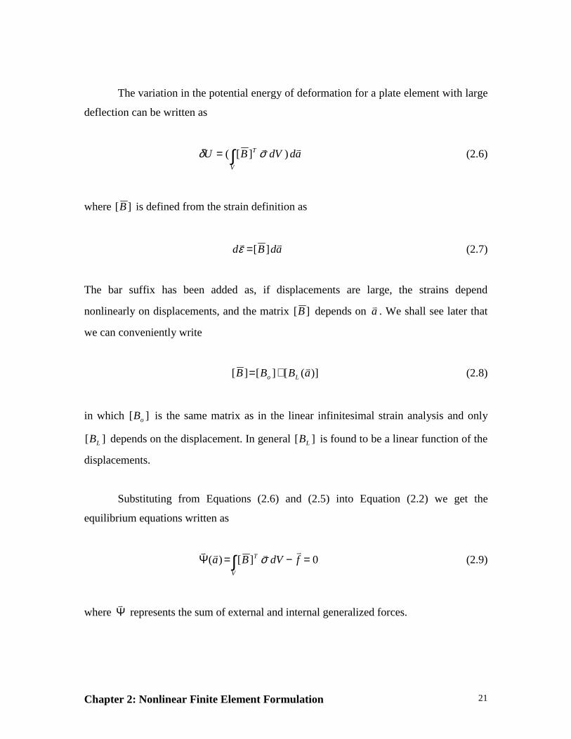
The variation in the potential energy of deformation for a plate element with large
deflection can be written as
addVBUV
T vv∫= )][( σδ (2.6)
where ][B is defined from the strain definition as
adBdvv
][=ε (2.7)
The bar suffix has been added as, if displacements are large, the strains depend
nonlinearly on displacements, and the matrix ][B depends on av
. We shall see later that
we can conveniently write
)]([][][ aBBB Lo
v+= (2.8)
in which ][ oB is the same matrix as in the linear infinitesimal strain analysis and only
][ LB depends on the displacement. In general ][ LB is found to be a linear function of the
displacements.
Substituting from Equations (2.6) and (2.5) into Equation (2.2) we get the
equilibrium equations written as
∫ =−=ΨV
T fdVBa 0][)(vvvv
σ (2.9)
where Ψv
represents the sum of external and internal generalized forces.
Chapter 2: Nonlinear Finite Element Formulation 22
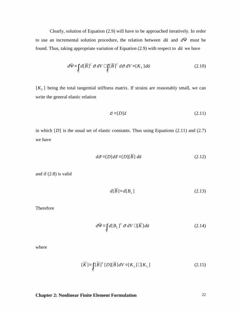
Clearly, solution of Equation (2.9) will have to be approached iteratively. In order
to use an incremental solution procedure, the relation between adv
and Ψv
d must be
found. Thus, taking appropriate variation of Equation (2.9) with respect to adv
we have
∫ ∫ =+=ΨV V
TTT adKdVdBdVBdd
vvvv][][][ σσ (2.10)
][ TK being the total tangential stiffness matrix. If strains are reasonably small, we can
write the general elastic relation
εσ vv][D= (2.11)
in which ][D is the usual set of elastic constants. Thus using Equations (2.11) and (2.7)
we have
adBDdDdvvv
][][][ == εσ (2.12)
and if (2.8) is valid
][][ LBdBd = (2.13)
Therefore
∫ +=ΨV
TL adKdVBdd
vvv][][ σ (2.14)
where
∫ +==V
LoT KKdVBDBK ][][][][][][ (2.15)

Chapter 2: Nonlinear Finite Element Formulation 23
In this expression ][ oK represents the usual, small displacement stiffness matrix, i.e.
∫=V
oT
oo dVBDBK ][][][][ (2.16a)
The matrix ][ LK is due to large displacements and is given by
∫ ++=V
oT
LLT
LLT
oL dVBDBBDBBDBK )][][][][][][][][][(][ (2.16b)
][ LK is alternatively known as the initial displacement matrix or large displacement
matrix, and contains only terms that are linear and quadratic in av
.
The first term of Equation (2.14) can be written as
∫ =V
TL adKdVBd
vv][][ σσ (2.17)
where ][ σK is a symmetric matrix dependent on the stress level. This matrix is known as
initial stress matrix or geometric matrix. Thus,
adKadKKKd TLo
vvv][)][][][( =++=Ψ σ (2.18)
with ][ TK being the total, tangential stiffness matrix.
In the next section, the tangential stiffness matrix for a rectangular plate element
is derived in terms of the element shape functions and nodal displacements.

Chapter 2: Nonlinear Finite Element Formulation 24
2.2 Stiffness Formulation for a Rectangular Plate Element
A typical rectangular laminated plate has dimensions a and b and thickness t. The
laminate is composed of a number of perfectly bounded orthotropic layers (laminae) with
different orientation angles. In a symmetric laminate, these laminae orientations are
placed symmetrically with respect to the mid-plane. A coordinate system is adopted such
that the x-y plane coincides with the mid-plane of the plate and the z-axis is perpendicular
to the plane.
The nonlinear stiffness formulations for large deflection analysis of plates with
initial imperfections are formulated for this typical rectangular plate finite element. The
element is shown in Figure (2.1) with six degrees of freedom at each nodal point. These
are : two inplane displacements u and v in the x and y directions, respectively; one
transverse deflection w; two rotations xw, and yw, about the y and x axes, respectively,
and a generalized twist xyw, .
Figure (2.1) Element geometry and nodal degrees of freedom
The present element is based on Kirchoff plate theory [77] which neglects
transverse shear deformation by assuming that straight lines normal to the mid-surface
before deformation remain straight and normal to the mid-surface after deformation.
a
b t
1 2
34
v w
wy
wx
wxy
u

Chapter 2: Nonlinear Finite Element Formulation 25
Knowing that the panels in this study have a width-to-thickness ratio of over 400, it is
thus clear that we can neglect the transverse shear deformation effects without any
significant loss in accuracy. The displacement model used in the formulation is thus
given as [77]
x
wzuu o ∂
∂−=
y
wzvv o ∂
∂−= (2.19)
oww=
where ooo wvu ,, are the mid-plane displacements in the x, y and z-direction, respectively.
Figure (2.2) shows the plate configuration before and after deformation. It is clear from
Equations (2.19) that the displacement at any point inside the plate can be expressed in
terms of five unknown quantities; yxooo wwwvu ,, ,,,, . However, the joint twist derivatives
xyw, are adopted as extra degrees of freedom to assure inclusion of the strain due to
simple twist.
Figure (2.2) Kirchoff thin plate deformation model
z, w
x, uz
p
t/2
dx
x, u
z, w
w
w,x
u = -z w,x
p

Chapter 2: Nonlinear Finite Element Formulation 26
2.2.1 Strain-Displacement Relations
The plate strains can be written in terms of the middle surface deflections as [78]
2
2
)2(2
1
x
wz
x
w
x
w
x
w
x
u ox ∂
∂−∂
∂+
∂∂
∂∂+
∂∂=ε
2
2
)2(2
1
y
wz
y
w
y
w
y
w
y
v oy ∂
∂−∂
∂+
∂∂
∂∂+
∂∂=ε (2.20)
yx
wz
x
w
x
w
y
w
y
w
y
w
x
w
x
v
y
u ooxy ∂∂
∂+∂
∂+
∂∂
∂∂+
∂∂
+∂∂
∂∂+
∂∂+
∂∂=
2
2)2(2
1)2(
2
1γ
where ow is the displacement function for the initial imperfection [78] and u, v, w stand
for appropriate displacements of the middle surface.
Or in a more compact form
{ }
++
+
−−
+
+=
xoyyox
yoy
xox
yx
y
x
xy
yy
xx
xy
y
x
wwww
ww
ww
ww
w
w
w
w
w
z
vu
v
u
,,,,
,,
,,
,,
2,
2,
,
,
,
,,
,
,
22
1
2
ε (2.21a)
Or
{ } { } { } { } { }pI
pL
bo
po z εεεεε +++= (2.21b)
where
{ }poε is the linear strain due to inplane deformation.
{ }boε is the linear strain due to bending deformation.
{ }pLε is the nonlinear strain due to inplane deformation.
{ }pIε is the nonlinear strain due to initial deformation.
Chapter 2: Nonlinear Finite Element Formulation 27
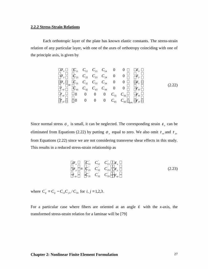
2.2.2 Stress-Strain Relations
Each orthotropic layer of the plate has known elastic constants. The stress-strain
relation of any particular layer, with one of the axes of orthotropy coinciding with one of
the principle axis, is given by
=
yz
xz
xy
z
y
x
symyz
xz
xy
z
y
x
CC
CC
CCCC
CCCC
CCCC
CCCC
γγγεεε
τττσσσ
.6665
5655
44434241
34333231
24232221
14131211
0000
0000
00
00
00
00
(2.22)
Since normal stress zσ is small, it can be neglected. The corresponding strain zε can be
eliminated from Equations (2.22) by putting zσ equal to zero. We also omit xzτ and yzτ
from Equations (2.22) since we are not considering transverse shear effects in this study.
This results in a reduced stress-strain relationship as
=
xy
y
x
xy
y
x
CCC
CCC
CCC
γεε
τσσ
’33
’32
’31
’23
’22
’21
’13
’12
’11
(2.23)
where 3333’ / CCCCC jiijij −= for 3,2,1, =ji .
For a particular case where fibers are oriented at an angle θ with the x-axis, the
transformed stress-strain relation for a laminae will be [79]
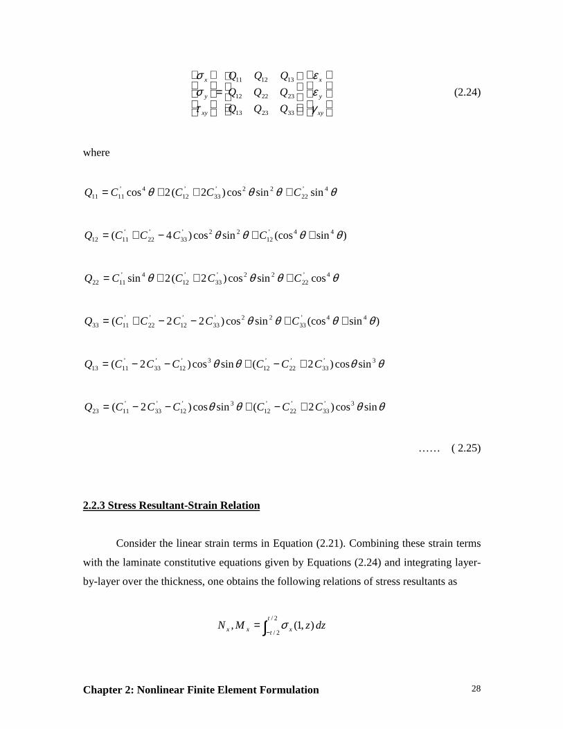
Chapter 2: Nonlinear Finite Element Formulation 28
=
xy
y
x
xy
y
x
QQQ
QQQ
QQQ
γεε
τσσ
332313
232212
131211
(2.24)
where
θθθθ 4’22
22’33
’12
4’1111 sinsincos)2(2cos CCCCQ +++=
)sin(cossincos)4( 44’12
22’33
’22
’1112 θθθθ ++−+= CCCCQ
θθθθ 4’22
22’33
’12
4’1122 cossincos)2(2sin CCCCQ +++=
)sin(cossincos)22( 44’33
22’33
’12
’22
’1133 θθθθ ++−−+= CCCCCQ
θθθθ 3’33
’22
’12
3’12
’33
’1113 sincos)2(sincos)2( CCCCCCQ +−+−−=
θθθθ sincos)2(sincos)2( 3’33
’22
’12
3’12
’33
’1123 CCCCCCQ +−+−−=
…… ( 2.25)
2.2.3 Stress Resultant-Strain Relation
Consider the linear strain terms in Equation (2.21). Combining these strain terms
with the laminate constitutive equations given by Equations (2.24) and integrating layer-
by-layer over the thickness, one obtains the following relations of stress resultants as
∫−=
2/
2/),1(,
t
t xxx dzzMN σ
Chapter 2: Nonlinear Finite Element Formulation 29
∫−=
2/
2/),1(,
t
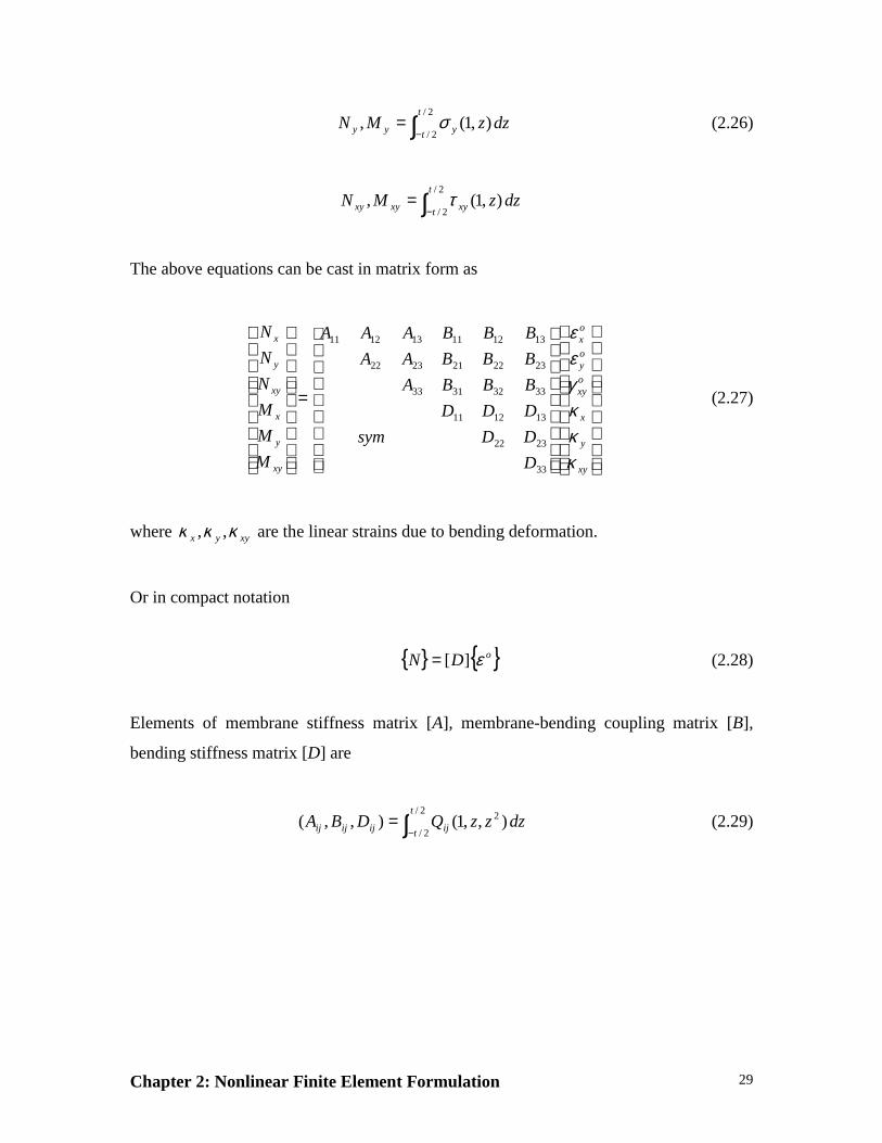
t yyy dzzMN σ (2.26)
∫−=
2/
2/),1(,
t
t xyxyxy dzzMN τ
The above equations can be cast in matrix form as
=
xy
y
x
oxy
oy
ox
xy
y
x
xy
y
x
D
DDsym
DDD
BBBA
BBBAA
BBBAAA
M
M
M
N
N
N
κκκγεε
33
2322
131211
33323133
2322212322
131211131211
(2.27)
where xyyx κκκ ,, are the linear strains due to bending deformation.
Or in compact notation
{ } { }oDN ε][= (2.28)
Elements of membrane stiffness matrix [A], membrane-bending coupling matrix [B],
bending stiffness matrix [D] are
∫−=
2/
2/
2 ),,1(),,(t
t ijijijij dzzzQDBA (2.29)
Chapter 2: Nonlinear Finite Element Formulation 30
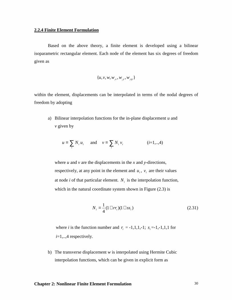
2.2.4 Finite Element Formulation
Based on the above theory, a finite element is developed using a bilinear
isoparametric rectangular element. Each node of the element has six degrees of freedom
given as
},,,,,{ ,,, xyyx wwwwvu
within the element, displacements can be interpolated in terms of the nodal degrees of
freedom by adopting
a) Bilinear interpolation functions for the in-plane displacement u and
v given by
∑=i
ii uNu and ∑=i
ii vNv (i=1,..,4)
where u and v are the displacements in the x and y-directions,
respectively, at any point in the element and iu , iv are their values
at node i of that particular element. iN is the interpolation function,
which in the natural coordinate system shown in Figure (2.3) is
)1)(1(4
1iii ssrrN ++= (2.31)
where i is the function number and ir = -1,1,1,-1; is =-1,-1,1,1 for
i=1,..,4 respectively.
b) The transverse displacement w is interpolated using Hermite Cubic
interpolation functions, which can be given in explicit form as
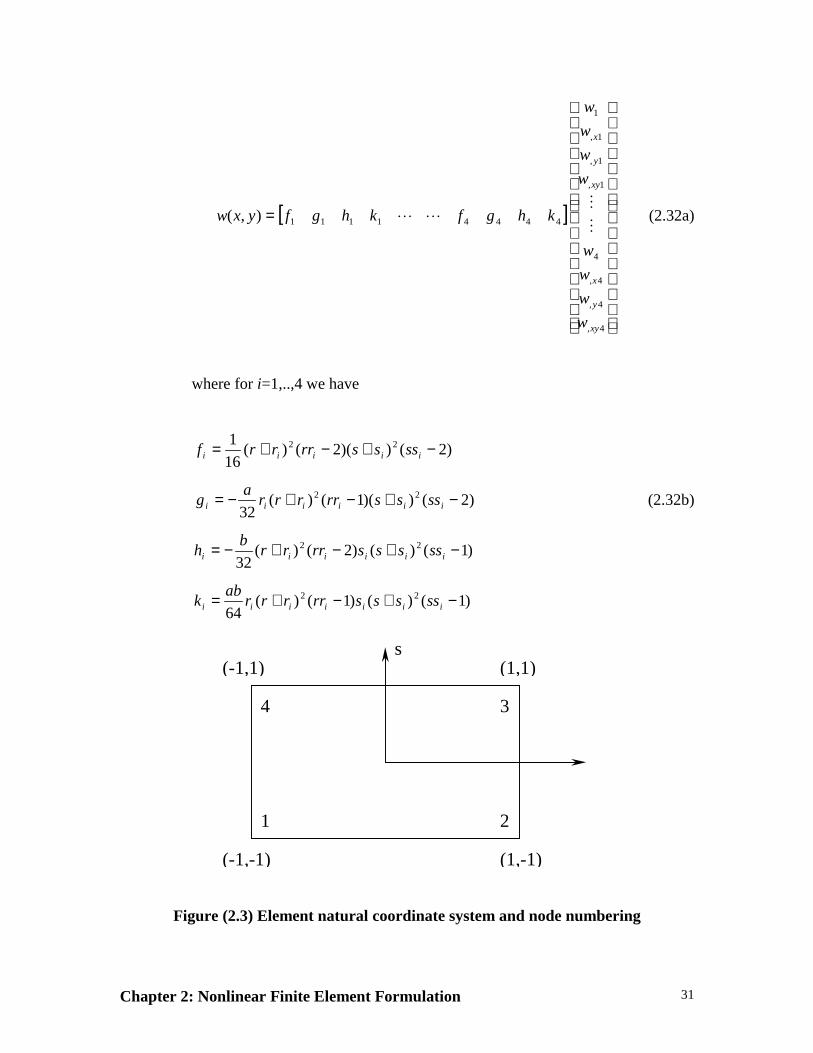
Chapter 2: Nonlinear Finite Element Formulation 31
[ ]
=
4,
4,
4,
4
1,
1,
1,
1
44441111),(
xy
y
x
xy
y
x
w
w
w
w
w
w
w
w
khgfkhgfyxwM
MLL (2.32a)
where for i=1,..,4 we have
)2())(2()(16
1 22 −+−+= iiiii ssssrrrrf
)2())(1()(32
22 −+−+−= iiiiii ssssrrrrra
g (2.32b)
)1()()2()(32
22 −+−+−= iiiiii sssssrrrrb
h
)1()()1()(64
22 −+−+= iiiiiii sssssrrrrrab
k
Figure (2.3) Element natural coordinate system and node numbering
(-1,-1) (1,-1)
(1,1)(-1,1)s
1 2
34
Chapter 2: Nonlinear Finite Element Formulation 32
Thus, we can express the displacement in terms of nodal degrees of freedom and
using the previously defined shape functions. For instance,
eaN
w
v
uv
][=
(2.33)
where eav
is the element nodal displacement vector and [N] is the matrix of shape
functions. For convenience the element nodal displacement vector eav
will be divided
into those which influence in-plane and bending deformation respectively.
=bi
pie
ia
aa v
vv
with
=i
ipi v
uav
and
∂∂∂∂∂∂∂
=
ii
i
i
i
bi
yx
wy
wx
ww
a
2
v (2.34)
Thus the shape functions can also be subdivided as
=
bi
pi
iN
NN
0
0][ (2.35)
2.2.5 Evaluation of the Linear Stiffness Matrix ][ oK
Substituting Equations (2.31) and (2.32) into the linear strain components of
Equation (2.21) we get
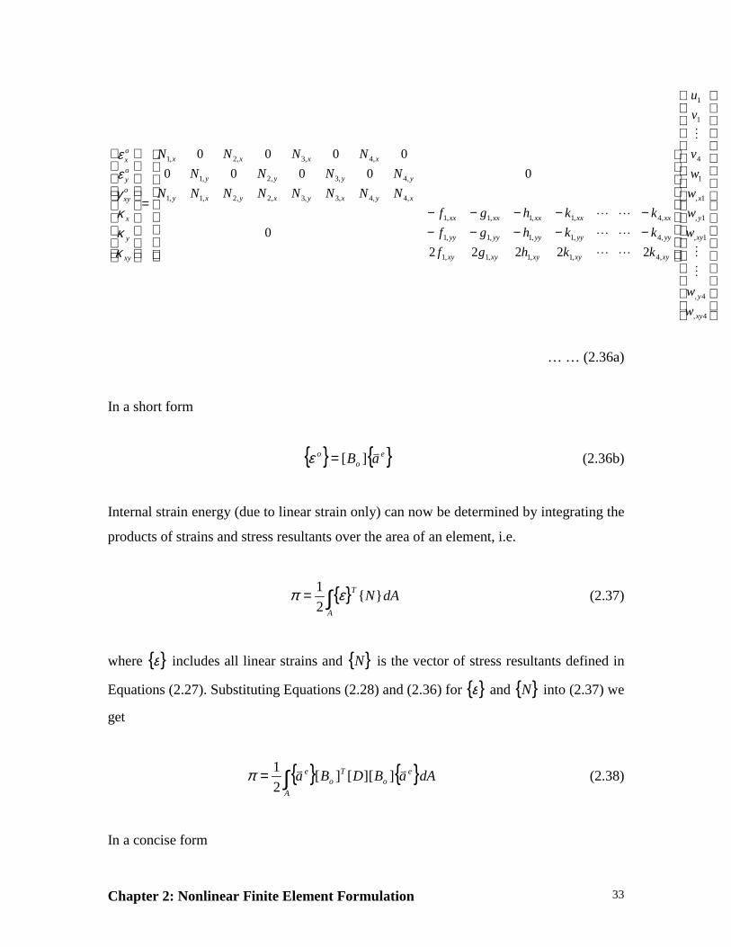
Chapter 2: Nonlinear Finite Element Formulation 33
−−−−−−−−−−
=
4,
4,
1,
1,
1,
1
4
1
1
,4,1,1,1,1
,4,1,1,1,1
,4,1,1,1,1
,4,4,3,3,2,2,1,1
,4,3,2,1
,4,3,2,1
22222
0
00000
0000
xy
y
xy
y
x
xyxyxyxyxy
yyyyyyyyyy
xxxxxxxxxx
xyxyxyxy
yyyy
xxxx
xy
y
x
oxy
oy
ox
w
w
w
w
w
w
v
v
u
kkhgf
kkhgf
kkhgf
NNNNNNNN
NNNN
NNNN
M
M
M
LL
LL
LL
κκκγεε
… … (2.36a)
In a short form
{ } { }eo
o aBv
][=ε (2.36b)
Internal strain energy (due to linear strain only) can now be determined by integrating the
products of strains and stress resultants over the area of an element, i.e.
{ }∫=A
T dAN}{2
1 επ (2.37)
where { }ε includes all linear strains and { }N is the vector of stress resultants defined in
Equations (2.27). Substituting Equations (2.28) and (2.36) for { }ε and { }N into (2.37) we
get
{ } { }∫=A
eo
To
e dAaBDBavv
][][][2
1π (2.38)
In a concise form
Chapter 2: Nonlinear Finite Element Formulation 34
{ } { }eo
Te aKavv
][2
1=π (2.39)
where
∫=A
oT
oo dABDBK ][][][][ (2.40)
is the linear stiffness matrix for the element.
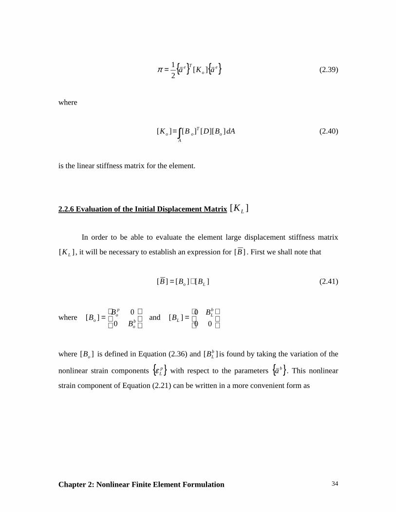
2.2.6 Evaluation of the Initial Displacement Matrix ][ LK
In order to be able to evaluate the element large displacement stiffness matrix
][ LK , it will be necessary to establish an expression for ][B . First we shall note that
][][][ Lo BBB += (2.41)
where
=
bo
po
oB
BB
0
0][ and
=
00
0][
bL
L
BB
where ][ oB is defined in Equation (2.36) and ][ bLB is found by taking the variation of the
nonlinear strain components { }pLε with respect to the parameters { }ba
v. This nonlinear
strain component of Equation (2.21) can be written in a more convenient form as
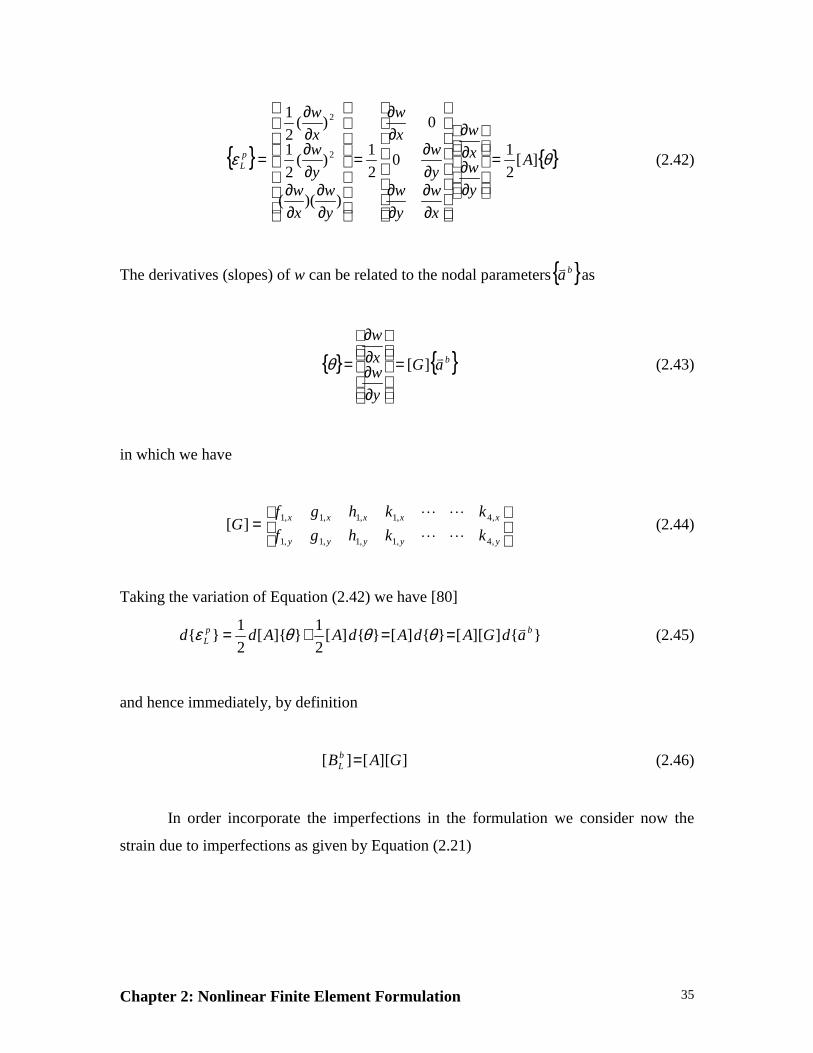
Chapter 2: Nonlinear Finite Element Formulation 35
{ } { }θε ][2
10
0
2
1
))((
)(2
1
)(2
1
2
2
A
y
wx
w
x
w
y
wy
wx
w
y
w
x
wy
wx
w
pL =
∂∂∂∂
∂∂
∂∂
∂∂
∂∂
=
∂∂
∂∂
∂∂∂∂
= (2.42)
The derivatives (slopes) of w can be related to the nodal parameters{ }bav
as
{ } { }baG
y
wx
wv
][=
∂∂∂∂
=θ (2.43)
in which we have
=
yyyyy
xxxxx
kkhgf
kkhgfG
,4,1,1,1,1
,4,1,1,1,1][
LL
LL(2.44)
Taking the variation of Equation (2.42) we have [80]
}{][][}{][}{][2
1}{][
2
1}{ bp
L adGAdAdAAddv==+= θθθε (2.45)
and hence immediately, by definition
][][][ GABbL = (2.46)
In order incorporate the imperfections in the formulation we consider now the
strain due to imperfections as given by Equation (2.21)
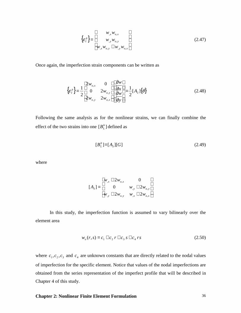
Chapter 2: Nonlinear Finite Element Formulation 36
{ }
+=
xoyyox
yoy
xoxpI
wwww
ww
ww
,,,,
,,
,,
ε (2.47)
Once again, the imperfection strain components can be written as
{ } { }θε ][2
1
22
20
02
2
12
,,
,
,
A
y
wx
w
ww
w
w
xoyo
yo
xopI =
∂∂∂∂
= (2.48)
Following the same analysis as for the nonlinear strains, we can finally combine the
effect of the two strains into one ][ bLB defined as
][][][ 3 GABbL = (2.49)
where
+++
+=
xoxyoy
yoy
xox
wwww
ww
ww
A
,,,,
,,
,,
3
22
20
02
][
In this study, the imperfection function is assumed to vary bilinearly over the
element area
srcscrccsrwo 4321),( +++= (2.50)
where 321 ,, ccc and 4c are unknown constants that are directly related to the nodal values
of imperfection for the specific element. Notice that values of the nodal imperfections are
obtained from the series representation of the imperfect profile that will be described in
Chapter 4 of this study.
Chapter 2: Nonlinear Finite Element Formulation 37
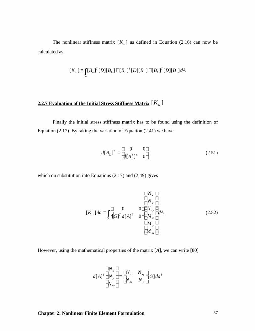
The nonlinear stiffness matrix ][ LK as defined in Equation (2.16) can now be
calculated as
∫ ++=A
oT
LLT
LLT
oL dABDBBDBBDBK ][][][][][][][][][][
2.2.7 Evaluation of the Initial Stress Stiffness Matrix ][ σK
Finally the initial stress stiffness matrix has to be found using the definition of
Equation (2.17). By taking the variation of Equation (2.41) we have
=
0][
00][ Tb
L
TL Bd
Bd (2.51)
which on substitution into Equations (2.17) and (2.49) gives
dA
M
M
M
N
N
N
AdGadK
xy
y
x
xy
y
x
ATT
= ∫ 0][][
00][
vσ (2.52)
However, using the mathematical properties of the matrix [A], we can write [80]
b
yxy
xyx
xy
y
xT adG
NN
NN
N
N
N
Adv
][][
=
Chapter 2: Nonlinear Finite Element Formulation 38
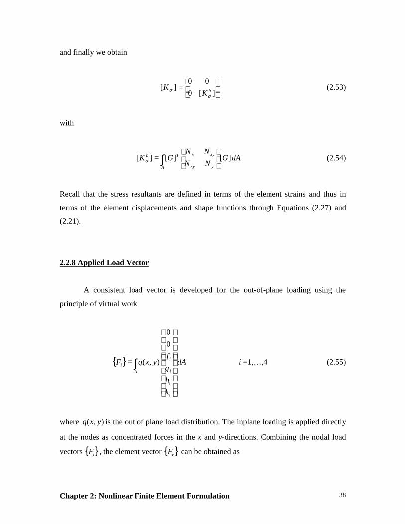
and finally we obtain
=
][0
00][ bK
Kσ
σ (2.53)
with
dAGNN
NNGK
A yxy
xyxTb ][][][ ∫
=σ (2.54)
Recall that the stress resultants are defined in terms of the element strains and thus in
terms of the element displacements and shape functions through Equations (2.27) and
(2.21).
2.2.8 Applied Load Vector
A consistent load vector is developed for the out-of-plane loading using the
principle of virtual work
{ } dA
k
h
g
fyxqF
A
i
i
i
ii ∫
=
0
0
),( i =1,…,4 (2.55)
where ),( yxq is the out of plane load distribution. The inplane loading is applied directly
at the nodes as concentrated forces in the x and y-directions. Combining the nodal load
vectors { }iF , the element vector { }eF can be obtained as

Chapter 2: Nonlinear Finite Element Formulation 39
{ } [ ]Te FFFFF 4321=
2.3 Hybrid Numerical-Analytical Integration
In order to perform the finite element analysis, the matrices defining element
properties, e.g. stiffness matrices, have to be computed. In a previous study by the author
[81], it was concluded that the use of analytical closed form integration (using symbolic
manipulation computer programs) in the evaluation of the element matrices in the linear
analysis case leads to a reduced computation time in addition to an increase in the
accuracy of the obtained results compared to the usual Gauss Quadrature integration
schemes [80]. However, in the present nonlinear analysis, the tangent stiffness matrix is
function of the element nodal degrees of freedom, which makes the use of analytical
integration out of reach due to the increased size of the expressions to be integrated. A
new hybrid integration technique that mixes both Gauss Quadrature and symbolic
manipulation together was introduced in this study.
To better describe the new technique, let’s consider the case of the linear stiffness
matrix given by
∫ ∫− −
=1
1
1
1
][][][4
][ drdsBDBab
K oT
oo
First, we start by evaluating the integrand in a closed form
][][][]ˆ[ oT
o BDBK = (2.56)
Notice that, terms of the matrix ]ˆ[K are functions of (r, s), element dimensions (a, b) and
element constitutive coefficients ijD .
Chapter 2: Nonlinear Finite Element Formulation 40
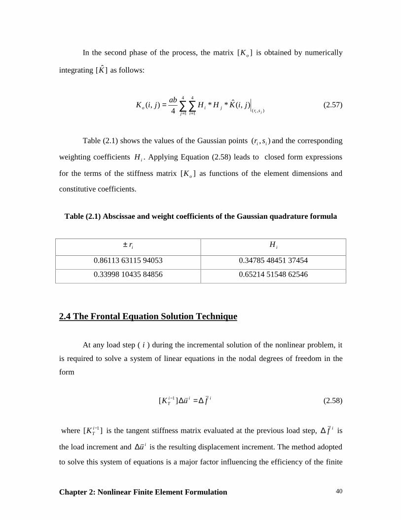
In the second phase of the process, the matrix ][ oK is obtained by numerically
integrating ]ˆ[K as follows:
∑∑= =
=4
1
4
1),(
),(ˆ**4
),(j i
srjio
ji
jiKHHab
jiK (2.57)
Table (2.1) shows the values of the Gaussian points ),( ii sr and the corresponding
weighting coefficients iH . Applying Equation (2.58) leads to closed form expressions
for the terms of the stiffness matrix ][ oK as functions of the element dimensions and
constitutive coefficients.
Table (2.1) Abscissae and weight coefficients of the Gaussian quadrature formula
ir± iH
0.86113 63115 94053 0.34785 48451 37454
0.33998 10435 84856 0.65214 51548 62546
2.4 The Frontal Equation Solution Technique
At any load step ( i ) during the incremental solution of the nonlinear problem, it
is required to solve a system of linear equations in the nodal degrees of freedom in the
form
iiiT fuK
vv ∆=∆− ][ 1 (2.58)
where ][ 1−iTK is the tangent stiffness matrix evaluated at the previous load step, if
v∆ is
the load increment and iuv∆ is the resulting displacement increment. The method adopted
to solve this system of equations is a major factor influencing the efficiency of the finite
Chapter 2: Nonlinear Finite Element Formulation 41
element program. Several options are open to the programmer ranging from iterative
methods such as the Gauss-Seidel technique [82] to the direct Gaussian elimination
algorithms. In this study we shall employ a direct elimination process and in particular
the frontal method of equation assembly and reduction. The frontal equation solution
technique was originated by Irons [83] and has earned the reputation of being easy and
inexpensive.
The frontal method can be considered as a particular technique for first
assembling finite elements stiffnesses and nodal forces into a global stiffness matrix and
load vector and then solving for the unknown displacement by means of a Gaussian
elimination and back substitution process. It is designed to minimize core storage
requirements, and the number of arithmetic operations.
No attempt will be made here to give a full detailed description of the frontal
technique. Such detailed presentation can be found in [84]. The frontal technique as
described in this study is applicable only to the solution of symmetric systems of linear
stiffness equations. Since the tangent stiffness matrix has been derived previously from a
variational principle, it is thus symmetric by definition [80]. Furthermore, even though
the problem is nonlinear by nature, we are using an incremental approach where the
system is transformed into a series of linearized systems of equations at each load
increment. This enables us to use the frontal technique at each load step.
The main idea of the frontal solver solution is to assemble the equations and
eliminate the variables at the same time. As soon as the coefficients of an equation are
completely assembled from the contributions of all relevant elements, the corresponding
variable can be eliminated. Therefore, the complete structural stiffness matrix is never
formed as such, since after elimination the reduced equation is immediately transferred to
back-up disc storage.
The core contains, at any given instant, the upper triangular part of a square
matrix containing the equations which are being formed at that particular time. These
Chapter 2: Nonlinear Finite Element Formulation 42
equations, their corresponding nodes and degrees of freedom are termed the front. The
number of unknowns in the front is the frontwidth; this length generally changes
continually during the assembly/reduction process. The maximum size of the problem
that can be solved is governed by the maximum frontwidth. The equations, nodes and
degrees of freedom belonging to the front are termed active; those which are yet to be
considered are inactive; those which have passed through the front and have been
eliminated are said to be deactivated.
During the assembly/elimination process the elements are considered each in turn
according to a prescribed order. Whenever a new element is called in, its stiffness
coefficients are read from a file and summed either into existing equations, if the nodes
are already active, or into new equations which have to be included in the front if the
nodes are being activated for the first time. If some nodes are appearing for the last time,
the corresponding equations can be eliminated and stored away in a file and are thus
deactivated. In so doing they free space in the front which can be employed during
assembly of the next element. More details concerning the technique are presented by
Hinton [84].
2.5 Incremental Procedure for Solution of Nonlinear Discrete Problems
The discretized nonlinear system of equations can be written as a set of algebraic
equations in the form
0)]([ =− faaKT
vvv(2.59)
where fv
is the external force and av
is the structural displacement. Both are generally
zero at the start of the problem. The incremental procedure makes use of the fact that the
solution for av
is known when the load term fv
is zero. In such circumstances, it is
convenient to study the behavior of av
as the vector fv
is incremented.
Chapter 2: Nonlinear Finite Element Formulation 43
Such a method can yield reasonable results and guaranteed to converge if a
suitably small increment of fv
is chosen. Furthermore, the intermediate results provide
useful information on the loading process.
To explain the method it is convenient to rewrite Equation (2.59) as
0)]([ =− oT faaKvvv λ (2.60)
where offvv
λ=
On differentiation of Equation (2.60) with respect to λ , this results in
0)]([ =− oT fd
adaK
vvv
λ(2.61a)
or
oT faKd
ad vvv
1)]([ −=λ
(2.61b)
where ][ TK is the tangential stiffness matrix previously described.
The problem posed in Equation (2.61b) is a classical one of numerical analysis for
which many solution (integration) techniques are available. The simplest one (Euler
method) states
iiT
io
iT
ii fKfaKaavvvvv ∆=∆=− −−+ 111 ][)]([ λ (2.62)
where the superscript refers to the increments of λ or fv
, i.e.,
Chapter 2: Nonlinear Finite Element Formulation 44
λλλ ∆+=+ ii 1
or (2.63)
fff iivvv
∆+=+1
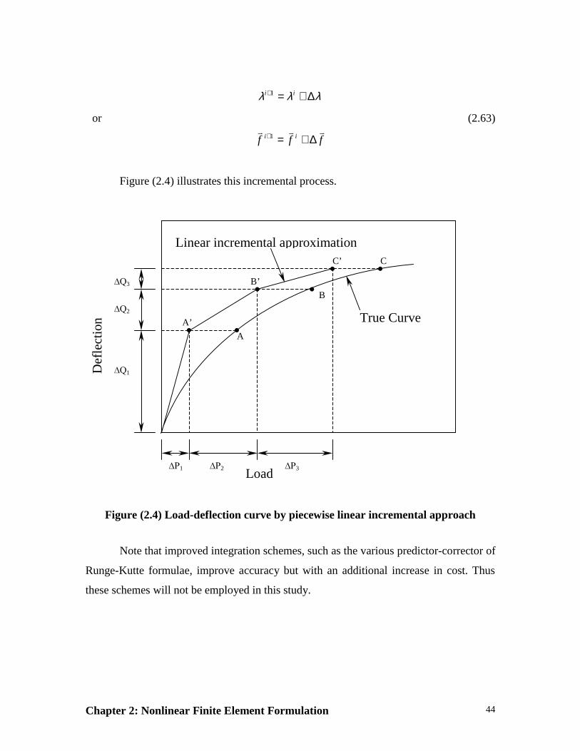
Figure (2.4) illustrates this incremental process.
Figure (2.4) Load-deflection curve by piecewise linear incremental approach
Note that improved integration schemes, such as the various predictor-corrector of
Runge-Kutte formulae, improve accuracy but with an additional increase in cost. Thus
these schemes will not be employed in this study.
A
A’
B
B’
CC’
¨31 ¨32 ¨33
¨41
¨42
¨43
Load
Def
lect
ion True Curve
Linear incremental approximation
Chapter 2: Nonlinear Finite Element Formulation 45
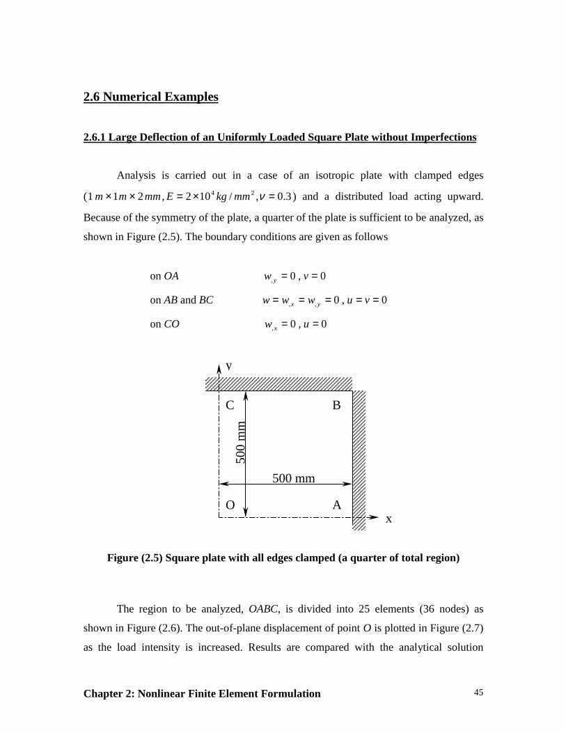
2.6 Numerical Examples
2.6.1 Large Deflection of an Uniformly Loaded Square Plate without Imperfections
Analysis is carried out in a case of an isotropic plate with clamped edges
( 3.0,/102,211 24 =×=×× νmmkgEmmmm ) and a distributed load acting upward.
Because of the symmetry of the plate, a quarter of the plate is sufficient to be analyzed, as
shown in Figure (2.5). The boundary conditions are given as follows
on OA 0,0, == vw y
on AB and BC 0,0,, ===== vuwww yx
on CO 0,0, == uw x
Figure (2.5) Square plate with all edges clamped (a quarter of total region)
The region to be analyzed, OABC, is divided into 25 elements (36 nodes) as
shown in Figure (2.6). The out-of-plane displacement of point O is plotted in Figure (2.7)
as the load intensity is increased. Results are compared with the analytical solution
A
BC
O
500 mm
500
mm
x
y

Chapter 2: Nonlinear Finite Element Formulation 46
obtained by S. Way [85]. A good agreement is observed. In Figure (2.8), upper and lower
fiber stresses at node O are shown and compared to the Finite Element nonlinear
solutions obtained by Kawai [88]. Finally the load intensity is fixed at 24 /108.0 mmkg−×
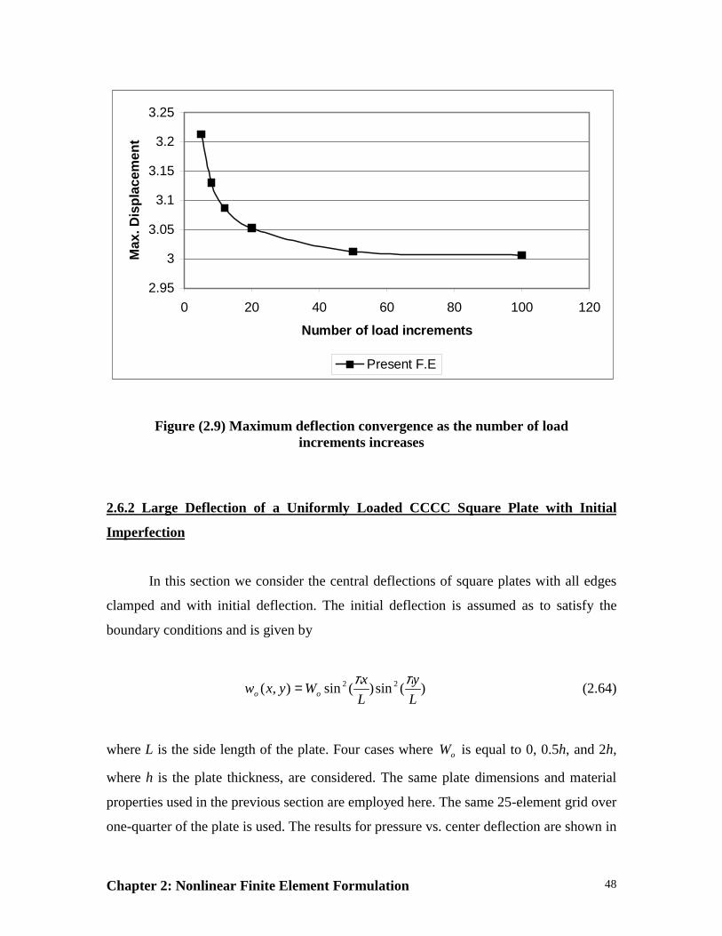
and the number of load increments used in the analyses is varied. Figure (2.9) shows the
convergence of the out of plane deflection at point O as the number of load increments
increases.
Figure (2.6) Finite element mesh employed
A
BC
Ox
y

Chapter 2: Nonlinear Finite Element Formulation 47
0.00E+00
5.00E-01
1.00E+00
1.50E+00
2.00E+00
2.50E+00
3.00E+00
3.50E+00
0 0.00002 0.00004 0.00006 0.00008 0.0001
Pressure (kg/mm2)
Cen
tral
Def
lect
ion
(m
m)
Current Nonlinear F.E Analytical Solution (S.Way)
Figure (2.7) Load-deflection curve at point O of a square plate with all edgesclamped under uniform load
-1
-0.5
0
0.5
1
1.5
2
0.0E+00 2.0E-05 4.0E-05 6.0E-05 8.0E-05 1.0E-04
Pressure (Kg/mm2)
σ x (
kg/m
m2 )
Present Analysis Upper Surface Present Analysis Lower Surface
FEM (Kawai) Upper Surface FEM (Kawai) Lower Surface
Figure (2.8) Upper and lower stress at point O of the square plate
Chapter 2: Nonlinear Finite Element Formulation 48
2.95
3
3.05
3.1
3.15
3.2
3.25
0 20 40 60 80 100 120
Number of load increments
Max
. Dis
pla
cem
ent
Present F.E
Figure (2.9) Maximum deflection convergence as the number of loadincrements increases
2.6.2 Large Deflection of a Uniformly Loaded CCCC Square Plate with Initial
Imperfection
In this section we consider the central deflections of square plates with all edges
clamped and with initial deflection. The initial deflection is assumed as to satisfy the
boundary conditions and is given by
)(sin)(sin),( 22
L
y
L
xWyxw oo
ππ= (2.64)
where L is the side length of the plate. Four cases where oW is equal to 0, 0.5h, and 2h,
where h is the plate thickness, are considered. The same plate dimensions and material
properties used in the previous section are employed here. The same 25-element grid over
one-quarter of the plate is used. The results for pressure vs. center deflection are shown in
Chapter 2: Nonlinear Finite Element Formulation 49
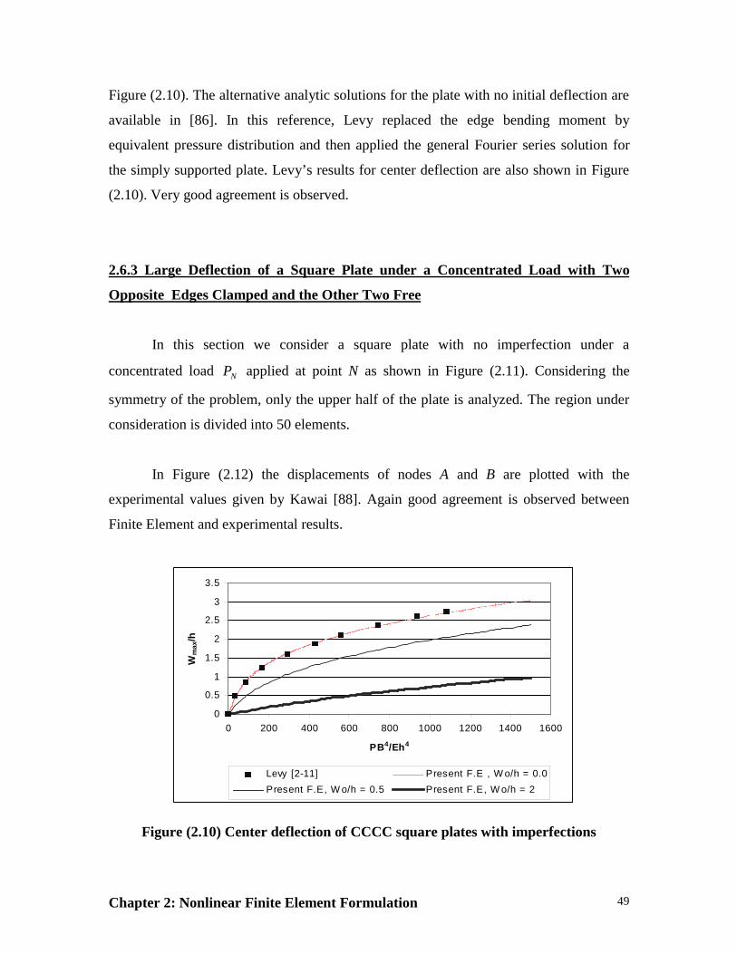
Figure (2.10). The alternative analytic solutions for the plate with no initial deflection are
available in [86]. In this reference, Levy replaced the edge bending moment by
equivalent pressure distribution and then applied the general Fourier series solution for
the simply supported plate. Levy’s results for center deflection are also shown in Figure
(2.10). Very good agreement is observed.
2.6.3 Large Deflection of a Square Plate under a Concentrated Load with Two
Opposite Edges Clamped and the Other Two Free
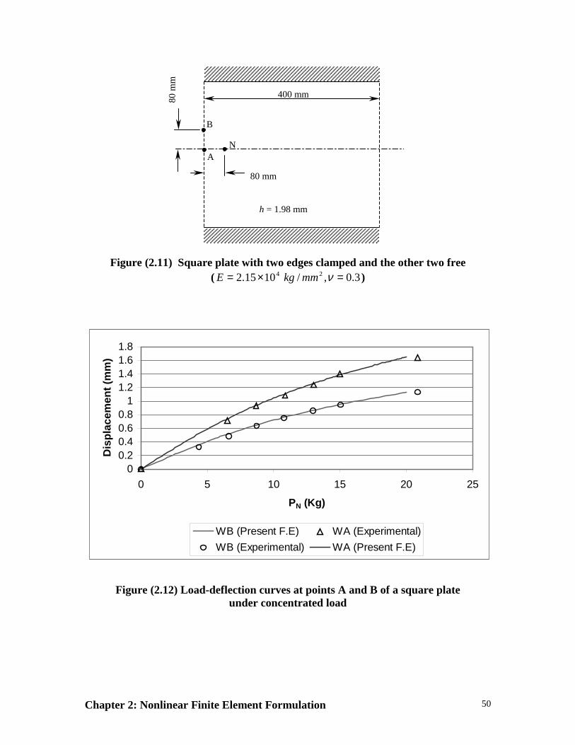
In this section we consider a square plate with no imperfection under a
concentrated load NP applied at point N as shown in Figure (2.11). Considering the
symmetry of the problem, only the upper half of the plate is analyzed. The region under
consideration is divided into 50 elements.
In Figure (2.12) the displacements of nodes A and B are plotted with the
experimental values given by Kawai [88]. Again good agreement is observed between
Finite Element and experimental results.
Figure (2.10) Center deflection of CCCC square plates with imperfections
0
0.5
1
1.5
2
2.5
3
3.5
0 200 400 600 800 1000 1200 1400 1600
PB4/Eh4
Wm
ax/h
Levy [2-11] Present F.E , W o/h = 0.0
Present F.E, W o/h = 0.5 Present F.E, W o/h = 2
Chapter 2: Nonlinear Finite Element Formulation 50
Figure (2.11) Square plate with two edges clamped and the other two free( 3.0,/1015.2 24 =×= νmmkgE )
00.20.40.60.8
11.21.41.61.8
0 5 10 15 20 25
PN (Kg)
Dis
pla
cem
ent
(mm
)
WB (Present F.E) WA (Experimental)
WB (Experimental) WA (Present F.E)
Figure (2.12) Load-deflection curves at points A and B of a square plateunder concentrated load
80 m
m
B
AN
80 mm
400 mm
h = 1.98 mm
Chapter 2: Nonlinear Finite Element Formulation 51
2.6.4 Postbuckling Response and Failure Prediction of Graphite-Epoxy Plates
Loaded in Compression
The postbuckling and failure characteristics of flat, rectangular graphite-epoxy
panels with and without holes that are loaded in axial compression have been examined
in an experimental study by Starnes and Rouse [89]. The panels were fabricated from
commercially available unidirectional Thornel 300 graphite-fiber tapes preimpregnated
with 450 K cure Narmco 5208 thermosetting epoxy resin. Typical lamina properties for
this graphite-epoxy system are 131.0 GPa for the longitudinal Young’s modulus, 13.0
GPa for the transverse Young’s modulus, 6.4 GPa for the inplane shear modulus, 0.38 for
the major Poisson’s ratio (12ν ), and 0.14 mm for the lamina thickness. Each panel was
loaded in axial compression using a 1.33-MN capacity hydraulic testing machine. The
loaded ends of the panel were clamped by fixtures during testing, and the unloaded edges
were simply supported by knife-edge restrains to prevent the panels from buckling as
wide columns. For more details about the test setup, or the experimental procedure, the
reader is referred to the paper by Starnes and Rouse [89].
In this study only one panel from Ref. [89] is analyzed, and the analytical results
are compared with the experimental results presented in Ref. [89]. The panel is 50.8 cm
long x 17.8 cm wide, 24-ply orthotropic laminate with a
s]90/0/450/450/45[ 22 ±±± stacking sequence. It is denoted as panel C4 in Ref.
[89]. Panel C4 was observed in the test to buckle into two longitudinal half-waves and
one transverse half-wave.
A finite element model for this panel was obtained using the element developed in
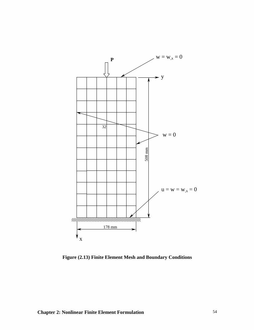
this study. The modeling approach was based on using six finite elements per buckle half
wave in each direction as recommended by Engelstad and Reddy [90]. Thus, six elements
were used along the width of the panel, while twelve elements were needed along the
length. The finite element mesh used is shown in Figure (2.13).
Chapter 2: Nonlinear Finite Element Formulation 52
In order to efficiently proceed beyond the critical buckling point in the
postbuckling analysis of the panel, an initial geometric imperfection in the same shape as
the first buckling mode was assumed. The amplitude of each mode was selected to be 1-
5% of the total laminate thickness. This means that an eccentricity is added to the initial
geometry that allows efficient progress past the critical point, but does not affect the
results in the postbuckling range.
Finally, the maximum strain criterion was used in this example to predict failure
of this panel. Failure occurs if any one of the following conditions are satisfied
tc cc or 1111 εεεε >>
tc cc or 2222 εεεε >> (2.65)
c1212 γγ >
where 21 ,εε are the normal strains along the fiber and normal to the fiber, respectively,
and 12γ is the in-plane shear strain. And cc 21 ,εε correspond to the critical strains in the 1
and 2-directions, and the subscripts t and c denote tension and compression, respectively.
Comparisons between test results from [89] and finite element results from the
present study are shown in Figures (2.14) and (2.15). End shortening u normalized by the
analytical end shortening cru at buckling is shown as a function of the applied load P
normalized by the analytical buckling load crP . The circles in this figure represent test
data, and the curve represent analytical data determined from the nonlinear finite element
analysis. A good correlation is observed between the experimental and the finite element
results. Figure (2.15) shows the out-of-plane deflection w near a point of maximum
deflection (node 32) normalized by the panel thickness t as a function of the normalized
load. Results obtained from a commercial finite element package (ABAQUS) are also
shown on the same figure. Notice that, in the ABAQUS analysis a curved shell element
Chapter 2: Nonlinear Finite Element Formulation 53
was employed in contrast to the flat shell element developed in this study, however the
total number of degrees of freedom was kept constant. From this graph we notice that the
postbuckling response of this panel exhibits large out-of-plane deflections (nearly three
time the panel thickness). This panel was analyzed by Reddy et al [91] using three
different finite element formulations, one of which utilized the classical laminated plate
theory with the effects of transverse shear neglected. In that work it was concluded that
the presence of shear flexibility improved the element convergence characteristics,
particularly when operating deep in the postbuckling regime. However, since we are
more concerned in this study with the cost of the analysis (this analysis is to be used for
optimization purposes), shear deformation will not be included in the formulation in
order to avoid the large increase in computation time associated with such an extension.
In this chapter we presented a 4 node, 24 degree of freedom rectangular element
for the geometrically nonlinear analysis of composite structures. A new integration
technique that mixes symbolic closed form function manipulation and Gaussian
quadrature numerical integration has been introduced in this study in order to reduce the
required computation time for each analysis. Several example problems were presented,
and finite element results were compared to analytical, experimental and other finite
element results. A very good agreement was demonstrated for problems involving
different sets of boundary conditions, loading and initial imperfection profiles. In the next
chapter FEPA is linked to a genetic algorithm in order to obtain a design tool (FEPAD).
Chapter 2: Nonlinear Finite Element Formulation 54
Figure (2.13) Finite Element Mesh and Boundary Conditions
508
mm
178 mm
y
x
w = 0
u = w = w,x = 0
w = w,x = 0P
32

Chapter 2: Nonlinear Finite Element Formulation 55
0.00E+00
5.00E-01
1.00E+00
1.50E+00
2.00E+00
2.50E+00
3.00E+00
0.00E+00
5.00E-01
1.00E+00
1.50E+00
2.00E+00
2.50E+00
3.00E+00
3.50E+00
4.00E+00
End Shortening, u/ucr
Lo
ad, P
/Pcr
Present F.E Experimental by Starnes [2-14]
Figure (2.14) Postbuckling response characteristics : End Shortening
0.00
0.50
1.00
1.50
2.00
2.50
0.00 0.50 1.00 1.50 2.00 2.50
w/t
P/P
cr
Experiment by Starnes [2-14] ABAQUS Present F.E
Figure (2.15) Postbuckling response characteristics : Out-of-plane deflection