7

CHAPTER 2 THEORY AND LITERATURE REVIEW

This research was focussed on the development of the synthetic methods and

characterisation (structural, thermal, magnetic and redox properties) of two types of

ionic copper(II) mixed carboxylates: (a) Ka[Cu2(p-OC6H4COO)a(CH3(CH2)nCOO)4-a],

and (b) [Cu2(p-H3NC6H4COO)a(CH3(CH2)14COO)4-a]Xa, where a = 1, 2; n = 14, 10, 8,

and 6; X = Cl, CH3COO and CF3SO3. These complexes were designed to be thermally

stable and magnetic metallomesogens and/or metal-containing ionic liquids. The latter

complexes were also designed to function as solvent-cum-catalysts in the carbon-carbon

bond-forming reaction of carbonyls. Accordingly, this chapter presents the relevant

theories and literature review related to this research.

2.1 Metallomesogens

Metallomesogens are also known as metal-containing liquid crystals [1-3]. These

materials combine the properties of liquid crystals (such as anisotropy and fluidity) with

those of metals (such as colour, magnetism, polarizability, multiple localized charges,

and variable geometries), which leads to the formation of mesophases which are

unobtainable in organic liquid crystals [1].

The liquid crystal state (termed mesophase) exists between the solid and liquid

states. Molecules (mesogens) of liquid crystals have the tendency to point along a

common axis (known as director). Hence, they contrast with molecules in the liquid

phase (which do not have intrinsic order) and in the solid state (which are highly

ordered with little translational freedom). Figure 2.1 shows the different arrangement of

molecules for each state.

8

Liquid crystals may be divided into two categories depending on how the

mesophase is formed: (a) thermotropic (temperature dependent). Most metallomesogens

are of this type); and (b) lyotropic (concentration and solvent dependent).

Thermotropic liquid crystals are made up of a central rigid core (for example, an

aromatic ring) and a flexible peripheral moiety (generally aliphatic groups). It can be

classified into two general classes: (a) calamitic or rod-like (possess elongated shape);

and (b) discotic or disc-like. Calamitic liquid crystals may exhibit two common types

of mesophases, namely nematic (N) and smectic (S).

The N phase is the least ordered mesophase (the closest to the isotropic liquid

state), where the molecules have only an orientational order (Figure 2.2).

The S phase posseses both an orientational and positional orders (layered

structures), and can be devided into many subclasses, such as smectic A (SA), where the

layers are perpendicular to the director, and smectic C (SC), when the director is tilted at

an angle to the normal (the z axis). Both phases are shown in Figure 2.3.

Figure 2.2 The nematic phase: (left) an illustration of the orientation of the molecules,

and (right) an optical micrograph of the characteristic Schlieren texture

Figure 2.1 Different molecular arrangement in (a) solid; (b) liquid crystal; and (c) liquid

(b)(a) (c)

9

Examples of SA and Sc phases are shown in Figure 2.4 and Figure 2.5

respectively.

Many calamitic systems are based on transition metals, which are capable of

forming complexes with a square planar or linear geometry. Figure 2.6 shows two

examples of these metallomesogens [4,5].

Figure 2.3 A molecular arrangement of: (a) SA phase; and (b) SC phase

Figure 2.4 An illustration of smectic A phase (left), and the optical texture of

the phase viewed under a polarizing microscope (right)

Figure 2.5 An illustration of smectic C phase (left) and the optical texture of the

phase viewed under a polarizing microscope (right)

10

CN M

Cl

Cl

NC OCnH2n+1CnH2n+1O

O

Cu

O

OO

CH3

H3C

OCnH2n+1

H2n+1CnO

The general structure of discotic (disc-shape) liquid crystals comprises of a

planar (usually aromatic) central rigid core surrounded by usually four, six or eight

flexible peripheries (mostly pendant chain). Hexa-substituted benzene derivatives

(Figure 2.7), synthesized by Chandrasekhar et al. [6] are the first series of organic

discotic compounds to exhibit mesophases.

O OO

OO O

ORRO

RO

ORR O O R

Discotic liquid crystals exhibit two main types of mesophases with varying degree

of organisation, namely nematic discotic (ND) and columnar (Col).

The ND phase is the least ordered mesophase as the molecules have only

orientational order (no positional order), as illustrated in Figure 2.8.

Figure 2.7 Molecular structure of the first series of discotic liquid crystals

discovered: benzene-hexa-n-alkanoate derivatives (R = C4H9 to C9H19)

Figure 2.6 Examples of calamitic metallomesogens

11

The Col phase is more ordered and has a tendency to stack one on top of another,

to form columns with different lattice patterns. As a results, a number of columnar

mesophases are identified, such as columnar rectangular (Colr) and columnar hexagonal

(Colh). These are illustrated in Figure 2.9.

Copper complexes of β-diketonates (Figure 2.10), which possess a square planar

geometry, are good examples of discotic metallomesogens [1].

O

Cu

O

O

O

R'R

RR'

O

Cu

O

O

O

ORRO

ORRO

ORRO

ORRO

Figure 2.8 An illustration of a molecular arrangement of ND phase

Figure 2.9 (a) The general structure of Col phases; (b) a representation of Colr;

and (c) a representation of Colh

Figure 2.10 Examples of discotic metallomesogens: (a) four-chain β-diketonates, and

(b) eight-chain β-diketonates

(a) (b)

12

Among the various metallomesogens already explored, binuclear carboxylates of

divalent transition metals, of general formula [M2(RCOO)4] where M = Cu(II), Rh(II),

Ru(II), Mo(II), and Cr(II), have been widely studied [7]. It is to be noted that all

binuclear carboxylates of this class exhibit the so-called ‘lantern’ or ‘paddle-wheel’

structure, exemplified by [Cu2(CH3COO)4(H2O)2] (Figure 2.11) [8].

Copper(II) salts of straight chain aliphatic carboxylates consist of columnar stacks

of dimers and hence showed discotic mesophases. Figure 2.12 shows the stacking of

these discotic molecules [9].

Figure 2.12 Lantern or paddle wheel structure of the dicopper(II) tetraalkanoate, stacking

in the two possible ways for the formation of the columnar phase: (a) tilted to the columnar

axis for the tetragonal phase; and (b) parallel to the columnar axis for the hexagonal phase

CuCuO

C OH3C O COCH3

OC OH3C

O CO CH3H2O

OH2Figure 2.11 Lantern or paddle-wheel structure of [Cu2(CH3COO)4(H2O)2]

(a) (b)

13

2.2 Metal-Containing Ionic Liquids

Ionic liquids (ILs) are defined as salts that melt at or below 100oC [10]. Ionic liquids

that are free-flowing at room temperature are called ambient temperature ionic liquids.

The initial interests in ILs arises mainly because of their possible use as ‘greener’

alternatives to volatile organic solvents. This is because these materials have relatively

low viscosities and exhibit very low vapour pressure under ambient conditions [10].

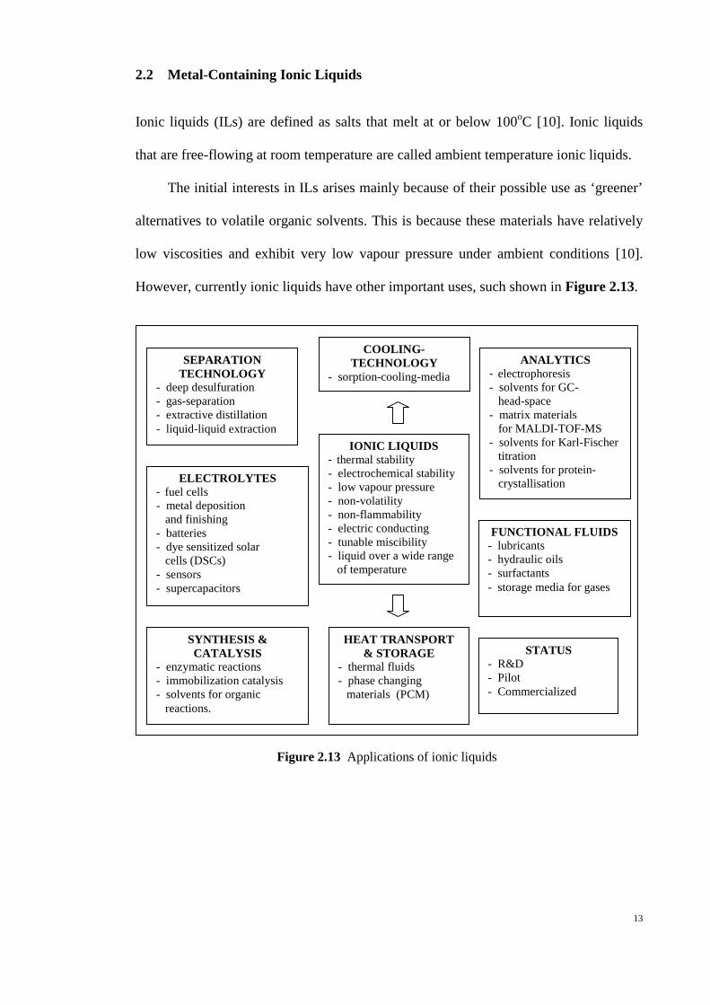
However, currently ionic liquids have other important uses, such shown in Figure 2.13.

IONIC LIQUIDS- thermal stability- electrochemical stability- low vapour pressure- non-volatility- non-flammability- electric conducting- tunable miscibility- liquid over a wide range of temperature

COOLING-TECHNOLOGY

- sorption-cooling-media

ANALYTICS- electrophoresis- solvents for GC- head-space- matrix materials for MALDI-TOF-MS- solvents for Karl-Fischer titration- solvents for protein- crystallisation

FUNCTIONAL FLUIDS- lubricants- hydraulic oils- surfactants- storage media for gases

STATUS- R&D- Pilot- Commercialized

SEPARATIONTECHNOLOGY

- deep desulfuration- gas-separation- extractive distillation- liquid-liquid extraction

ELECTROLYTES- fuel cells- metal deposition

and finishing- batteries- dye sensitized solar

cells (DSCs)- sensors- supercapacitors

HEAT TRANSPORT& STORAGE

- thermal fluids- phase changing

materials (PCM)

SYNTHESIS &CATALYSIS

- enzymatic reactions- immobilization catalysis- solvents for organic reactions.

Figure 2.13 Applications of ionic liquids

14

Currently, most research on ionic liquids are based on cations, namely

imidazolium, ammonium and pyridinium (known as nitrogen-based ILs), and on

phosphonium cores (Figure 2.14).

NNR1 R2

N

R

N

R2

R2 R2

R1

P

R2

R2 R2

R1

The anions are mainly inorganic species, such as [BF4-], [PF6

-], [X-], [NO3-],

[OH-], [CN-], and halometallates [MXnm-], where X is an halide. Examples of organic

anions are [RCOO-] and [CF3SO3-] [10].

Metal-containing ionic liquids (MetILs) (Figure 2.15) are a large class of highly

modifiable molten salts [11]. They offer the possibility of more highly charged species

(for example, [LnX63-]) and additional variations in geometries (examples, tetrahedral

and square planar [MX42-]) [12].

N NC7H15

2

NiCl4

The important characteristics of metal-containing ionic liquids are high thermal

stability, negligible vapour pressure, wide electrochemical window and the ability to

dissolve a range of organic and inorganic compounds. These have been exploited in the

context of separations, catalysis and electrochemistry [11].

Figure 2.15 An example of a metal-containing ionic liquid [12]

Figure 2.14 Examples of cations of ionic liquids

dialkylimidazolium alkylpyridinium tetraalkylphosphoniumtetraalkylammonium

15

2.3 Copper(II) Carboxylates

The chemistry of copper(II) complexes has received a great deal of attention in several

different fields, ranging from catalysis to bioinorganic and material chemistry. Copper

is a transition metal with the electronic configuration [Ar]3d104s1. It commonly forms

complexes as Cu+ (3d10) or Cu2+ (3d9) ions, and in some rare cases, as Cu3+ (3d8) ion.

Cu2+ is the most stable and important ion for copper and plays a crucial role in several

characterization methods of the complexes formed, such as electronic spectroscopy,

magnetic susceptibility and electron paramagnetic resonance spectroscopy [13].

Copper(II) carboxylates are made up of central copper(II) bonded to a fix numbers

of carboxylate ions (oxygen donor ligands), by coordinated covalent bonds [14].

Carboxylate anions are versatile ligands because each of its oxygen atom carries two

lone pairs. Various coordination modes are thus possible [15] (Figure 2.18; shown

later). It is noted that diverse structures of these complexes have been reported, such as

mononuclear, binuclear and polynuclear [13].

However, most copper(II) carboxylates have the dinuclear paddle-wheel structure

(Figure 2.11). This is the structure adopted by copper(II) acetate [8], and the structure

suggested for other copper(II) carboxylates, such as copper(II) butanoate, copper(II)

hexanoate, copper(II) octanoate and copper(II) decanoate [9]. The structure consists of

a dimer made up of two copper(II) ions bonded to four bridging bidentate carboxylates.

As such, there is a significant electronic and magnetic communications between the two

unpaired electrons on the copper(II) centres, and allows ready delocalization of

electrons [16].

In the dinuclear paddle-wheel structure, only one of the lone pairs of each oxygen

atom is involved in coordination. However, stepped polymeric structure may also form

(Figure 2.16) [15].

16

CuO

O OO

CuO

O OO

CC RR

C R

CR

CuO

O OO

CuO

O OO

CC RR

C R

CR

L L

CuO

O OO

CuO

O OO

CC RR

C R

CR

CuO

O OO

CuO

O OO

CC RR

C R

CR

L

CuO

O OO

CuO

O OO

CC RR

C R

CR

CuO

O OO

CuO

O OO

CC RR

C R

CR

2.4 The C-C Bond-Forming Reactions

The formation of a carbon-carbon bond is very important to the success of synthetic

organic chemistry. An example is the aldol reaction of carbonyls (aldehydes and

ketones), proposed to proceed by two different mechanisms: (a) enol; and (b) enolate

mechanisms.

In the enol mechanism, the carbonyl compounds are converted to enols or enol

ethers. These compounds, being nucleophilic at the α-carbon, can attack especially

reactive protonated carbonyls [17].

In the enolate mechanism, the carbonyl compounds, being carbonic acids, are

deprotonated to form enolates, which are much more nucleophilic than enols or enol

ethers, and therefore can attack electrophiles directly. The usual electrophile is an

aldehyde, since ketones are much less reactive. Both enol and enolate mechanisms are

shown in Figure 2.17 [17].

Figure 2.16 General structure of polynuclear copper(II) carboxylates: (I) stepped

without additional ligands; (II) ligands bridging two Cu; and (III) ligands bridging Cu

and O

I II III

17

Recently, it was accidentally discovered that copper(II) arylcarboxylates reacted

with acetone in the presence of HCl, to form black solids [18]. These solids were

soluble in most organic solvents, insoluble in water, have physical characteristic tuned

by the arylcarboxylates used, were redox active, and thus potential low band-gap

photonic materials and redox catalysts. One of the component of these solids were a

product formed in the C-C bond forming product of acetone molecules. Thus, this

reaction would serve as a new and facile synthetic method for such industrially

important organic products.

2.5 Elemental Analyses

Elemental analyses is the determination of the mass fractions of carbon, hydrogen,

nitrogen, and heteroatoms (X) (halogens, sulfur) of a sample. The results helps in the

determination of the chemical formula of an unknown substance.

CHN analysis is the most common form of elemental analyses. The technique

used involves combustion; a sample is burned in an excess of oxygen, and the products

of the combustion, carbon dioxide, water, and nitric oxides, are collected by various

traps. The masses of these combustion products may be used to calculate the percentage

Figure 2.17 The enol (top) and enolate (bottom) mechanisms of aldol condensation

of carbonyl compounds

18

composition of the unknown sample, and then the empirical formula (the simplest

whole-number ratios of the elements) [19].

2.6 Fourier Transform Infrared Spectroscopy

Fourier transform infrared spectroscopy (FTIR) is an important tool to identify

functional groups and types of chemical bonds in a molecule. It involved infrared

radiation between 4000 cm-1 to 400 cm-1 (between the visible and microwave regions in

the electromagnetic spectrum).

It is based on the principle that almost all molecules absorb infrared light only at

certain frequencies, where it affects the dipolar moment of the molecule. The data is

collected and converted from an interference pattern to the absorption spectrum which

provides a unique characteristic for each molecule.

For metal carboxylates, FTIR spectra are additional useful as it may be used to

determine the coordination mode of the carboxylate ligands. In metal complexes, a

carboxylate ion, RCOO-, can coordinate to metals mainly as monodentate, chelating or

bridging bidentate (syn-syn, syn-anti or anti-anti configuration) ligands (Figure 2.18).

O CO RMOCO RM

O CO RM

M O CO RM

MO CO RMM

Figure 2.18 Coordination of carboxylate ligand: (I) monodentate; (II) chelating;

amd (III) bridging bidentate: (a) syn-syn, (b) syn-anti, (c) anti-anti

I

III.a

II

III.b III.c

19

The type of binding mode is deduced from the ∆ value (the separation between the

two carboxylate stretching modes, ν(COO) asym and ν(COO)sym). The ∆ values of greater

than 200 cm-1 indicate a monodentate coordination [21], those between 120 cm-1 to 180

cm-1 indicate a bridging coordination [22,31], while those lower than 120 cm-1 indicate

a chelating coordination. The assessment of the relationship was initially based on the

infrared data of acetato and trifluoroacetato complexes, which were later extended to

other alkyl or aryl carboxylate ions [20].

2.7 UV-Visible Spectroscopy

UV-vis spectroscopy involves measurements of light absorbed at wavelength within the

ultraviolet (200-400 nm), visible (400-700 nm) and near infrared (700-1000 nm) regions

of the electromagnetic spectrum. The energies within these wavelengths are sufficient to

excite an electron to higher energy orbitals.

Most transition metal complexes are coloured due to the electronic transitions

(either d-d or charge transfer). A d-d transition involves the excitation of an electron in

a d orbital of a metal by a photon of visible light, to another higher energy d orbital (the

excited state). Only light with wavelengths (λ) that exactly match the energy difference

between the ground and the excited states will be absorbed. When this happens, the

light that is not absorbed is transmitted, and gives the colour of the complex (which is

on the opposite side of the colour that is absorbed – refer to the colour wheel, Figure

2.19). For example, a substance that absorbs light of wavelength 600-620 nm appears

blue, while that that absorps at 680-700 nm appears green.

20

A charge transfer band is due to the excitation of an electron, either from a metal-

based orbital into an empty ligand-based orbital (known as metal-to-ligand charge

transfer - MLCT), or from a ligand-based orbital into an empty metal-based orbital

(known as ligand-to-metal charge transfer - LMCT).

When UV-visible radiation is passed through a solution contained in a cell of path

length, l, some of the radiation is absorbed while others is transmitted. The transmitted

radiation has a certain intensity, I. If only the solvent is contained in the cell, the

transmitted radiations has an intensity, Io. The ratio of I to Io is known as transmittance,

T of the sample. The relationship is:

T = I/Io

An exponential curve is obtained when T is plotted against l. A linear graph is

obtained when a logarithmic function of T is used. Absorbance, A, which is the amount

of light absorbed by substance, is defined as:

A = log (1/T) = log Io/I

where A is the absorbance.

The relationship between the absorbance, concentration and path length is

known as Beer-Lambert’s law:

Figure 2.19 The colour wheel

21

A = εcl

where ε is the molar absorptivity, c is the concentration in mol dm-3 and l is the path

length in cm. A recording of A as a function of the wavelength produces the absorbance

spectrum.

The UV-vis absorption spectra are very useful in providing information on the

geometry of metal complexes, deduce from the wavelength of the d-d band (λmax,

wavelength of absorption maxima). For copper(II) complexes, the expected λmax for a

tetrahedral complex is normally at about 800 nm, a square pyramidal complex at about

700 nm [23,24], and a square planar complex at about 600 nm [25].

The crystal-field theory (CFT) can be used to explain the electronic structure of

metal complexes. This is done by determining the energy changes of five degenerate d

orbitals (Figure 2.20) when surrounded by ligands (illustrated as an array of point

charges).

As a ligand approaches the metal ion, the electrons in the d orbitals and in the

ligand experiences repulsion. As a result, the d electrons closer to the ligands will have

higher energy than those further away. Thus, the five d orbitals loss its degeneracy. The

Figure 2.20 Shapes (angular dependence functions) of the d orbitals

22

splittings of the d orbitals for tetrahedral, octahedral, and square planar complexes are

shown in Figure 2.21.

An octahedral complex has six ligands, forming an octahedron around the metal

ion. In this situation, the d orbitals split into two sets: two higher-energy orbitals, termed

eg (dz2 and dx

2-y

2), and three lower-energy orbitals, termed t2g (dxy, dxz and dyz). The

energy difference, Δoct, is known as the crystal-field splitting parameter.

A tetrahedral complex has four ligands, forming a tetrahedron around the metal

ion. The energy splitting is the opposite of that of an octahedral complex. The d orbitals

split into three higher energy orbitals, termed t2 (dxy, dxz and dyz), and two lower energy

orbitals, termed e (dz2 and dx

2-y

2). The energy difference is Δtet, which is lower (about 4/9

Δoct). This is because there are only four ligands and that the ligand electrons are not

oriented directly towards the d orbitals.

Many complexes experience geometrical distortion. This is explained by the Jahn-

Teller theorem, published in 1937, which states that “any non-linear molecular system

Figure 2.21 Splitting of d orbitals for tetrahedral, octahedral and square planar

complexes

23

in a degenerate electronic state will be unstable and will undergo distortion to form a

system of lower symmetry and lower energy, thereby removing the degeneracy” [26].

For copper(II) complexes(d9 configuration), the dz2 and dx

2-y

2 orbitals are unequally

occupied. To minimize repulsion with the ligands, two electrons occupy the dz2 orbital

and one electron occupy the dx2-y

2 orbital. Consequently, there is a stronger repulsion

along the z-axis. Hence, most copper(II) complexes have an elongation along the z-axis,

which leads to square planar geometry.

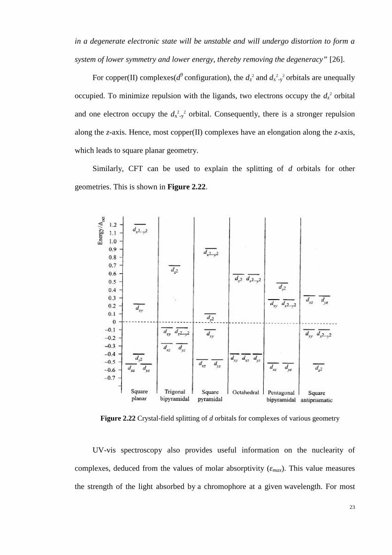
Similarly, CFT can be used to explain the splitting of d orbitals for other

geometries. This is shown in Figure 2.22.

UV-vis spectroscopy also provides useful information on the nuclearity of

complexes, deduced from the values of molar absorptivity (εmax). This value measures

the strength of the light absorbed by a chromophore at a given wavelength. For most

Figure 2.22 Crystal-field splitting of d orbitals for complexes of various geometry

24

mononuclear copper(II) complexes, the values of εmax are about 100 M-1 cm-1 [27,28].

Hence a value of greater than 200 M-1cm-1 suggests two Cu(II) chromophores [29].

2.8 Thermal Analyses

Thermal analyses involve the study of properties of materials with changes of

temperature. Two examples are thermogravimetry and differential scanning calorimetry.

2.8.1 Thermogravimetric Analysis

Thermogravimetric analysis (TGA) measures the amount of weight loss (in %) of a

sample as a function of temperature in a controlled atmosphere (inert gas, N2) up to

900oC.

The analyzer consists of a high-precision balance with a pan loaded with the

sample, placed in a small oven with a thermocouple (electrically heated), to measure

the temperature accurately. To control the instrument, a computer is connected to the

analyzer.

The results are displayed as a TGA curve (thermogram) in which weight % is

plotted against temperature. It is used to determine the thermal stability, the

decomposition process and the amount of residue left at the end of the experiment.

As an example, the thermogram of a sample of copper(II) benzoate,

[Cu2(C6H5COO)4(CH3CH2OH)2] is shown in Figure 2.23 [16]. It shows that the sample

was thermally stable up to around 230oC. It then decomposed in a two-step process. The

initial weight loss of 7.4% at 81.7oC is assigned to the loss of CH3CH2OH at the axial

positions (expected 9.7%). The total weight loss of 68.3% (expected 68.8%) is assigned

to the decomposition of the carboxylates ligands to CO2 and other volatiles.

For many copper(II) carboxylates, it has been suggested that the residue is mainly

copper(II) oxide [23,30]. By using the gravimetry concept, the formula mass of metal

25

complexes may be calculated. Thus, the TGA can be an alternative technique used to

support the proposed structure of a complex, in the absence of crystal data.

2.8.2 Differential Scanning Calorimetry

Differential scanning calorimetry (DSC) is used mainly in studying the phase

transitions, such as fusion and crystallization, glass transition, melting and clearing

temperatures (Figure 2.24). During the phase transition, more or less heat will flow to

the sample than the reference (an inert material such as empty aluminium pan), to

maintain both at the same temperature. It depends on whether the process is

endothermic (heat is absorbed, such as melting and glass transition), or exothermic (heat

is released, such as crystallization and formation of a chemical bond).

Figure 2.23 TG and DTA curves of [Cu2(C6H5COO)4(C2H5OH)2]

26

The amount of heat absorbed or released is measured, and the result is recorded as

a curve of heat flow versus temperature. It is then used to calculate enthalpies of

transitions (ΔH). The reaction is either endothermic (ΔH = positive) or exothermic

(ΔH = negative).

2.9 Optical Polarizing Microscopy

Optical polarising microscopy (OPM) is useful in providing information on the phase

transition and the study of mesomorphism of liquid crystals. It is designed to observe

and photograph samples that are visible due to their optically anisotropy.

For the identification of the liquid crystalline mesophases, the texture observed by

is analyzed and compared with published results. Some examples of liquid crystal phase

textures are shown in Figure 2.25 [32].

Figure 2.24 An example of a DSC curve

27

For copper(II) linear alkylcarboxylates with 4 to 21 carbon atoms, a phase

transition from lamellar crystalline solid to a hexagonal liquid-crystalline phase is

observed [33] (Figure 2.26).

(c)

(d)

(b)(a)

(e) (f)

Figure 2.25 OPM textures of different phases of liquid crystals: (a) N droplets;

(b) N; (c) cholesteric; (d) SA ; (e) Dh; and (f) spherulite texture of a crystalline phase

Figure 2.26 A schematic view of the columnar mesophase of copper(II) linear

alkylcarboxylates. Each column is made of stacked dicopper tetracarboxylate units.

28

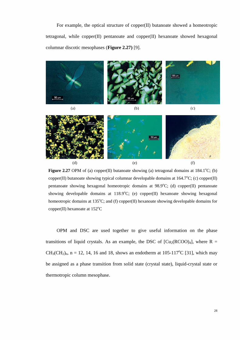
For example, the optical structure of copper(II) butanoate showed a homeotropic

tetragonal, while copper(II) pentanoate and copper(II) hexanoate showed hexagonal

columnar discotic mesophases (Figure 2.27) [9].

OPM and DSC are used together to give useful information on the phase

transitions of liquid crystals. As an example, the DSC of [Cu2(RCOO)4], where R =

CH3(CH2)n, n = 12, 14, 16 and 18, shows an endotherm at 105-117oC [31], which may

be assigned as a phase transition from solid state (crystal state), liquid-crystal state or

thermotropic column mesophase.

(c)

(d)

(b)(a)

(e) (f)

Figure 2.27 OPM of (a) copper(II) butanoate showing (a) tetragonal domains at 184.1oC; (b)

copper(II) butanoate showing typical columnar developable domains at 164.7oC; (c) copper(II)

pentanoate showing hexagonal homeotropic domains at 98.9oC; (d) copper(II) pentanoate

showing developable domains at 118.9oC; (e) copper(II) hexanoate showing hexagonal

homeotropic domains at 135oC; and (f) copper(II) hexanoate showing developable domains for

copper(II) hexanoate at 152oC

29

2.10 Magnetic Susceptibility

Magnetic properties of materials are studied by applying a magnetic field and measuring

the induced megnetization. Some materials are repelled (diamagnetism), others are

attracted to a magnetic field (paramagnetism).

Diamagnetic materials have no net magnetic moments because they do not have

unpaired electrons. The magnetic fields are produced from the tiny current loops created

by orbital motions of the electrons. When an external magnetic field is applied, these

current loops are aligned to oppose the applied field producing a negative magnetization

and thus negative susceptibility.

Paramagnetic materials have permanent magnetic moments (dipoles) due to the

spin of unpaired electrons. When a magnetic field is applied, the dipoles are aligned in

the same direction of the applied field, resulting in a net positive magnetic moment and

positive susceptibility.

In the absence of an external field, the dipoles do not interact with one another and

are randomly oriented due to thermal agitation (Figure 2.28).

In a short-ranged, the individual spins often interact with neighbouring spins in a

cooperative fashion, where the direction of one spin influences the directions of its

neighbouring spins. However, in bulk, it can cause a long-range magnetic ordering in

the absence of applied field below a certain critical temperature.

Figure 2.28 Random orientation of magnetic moments in paramagnetic materials

30

There are three basic types of bulk magnetic properties: ferromagnetism,

antiferromagnetism and ferrimagnetism. Ferromagnetism is the strongest and most

common type of magnetism. Ferromagnetic material has unpaired electrons. In the

absence of an external magnetic field, its magnetic moments (dipoles) has a tendency to

orient parallel to each other to maintain a lowered-energy state. As a result, the material

exhibit spontaneous magnetization (a net magnetic moment) as shown in Figure 2.29.

Above the Curie temperature, TC (a constant for every ferromagnetic substance),

the electrons in the bonds are unable to keep the dipole moments aligned (due to the

violent thermal motion), causing the material to lose its ferromagnetic properties and

changes into a paramagnetic material.

In an antiferromagnetic material, the intrinsic magnetic moments of neighbouring

valence electrons are aligned in the opposite directions (anti-aligned) (Figure 2.30),

resulting in zero net magnetic moment. The antiferromagnetic properties exist at

sufficiently low temperatures. Above the Néel temperature (TN) the material is

typically paramagnetic.

Figure 2.30 Alignment of magnetic moment in antiferromagnetic materials

Figure 2.29 Parallel alignment of magnetic moment in ferromagnetic materials

31

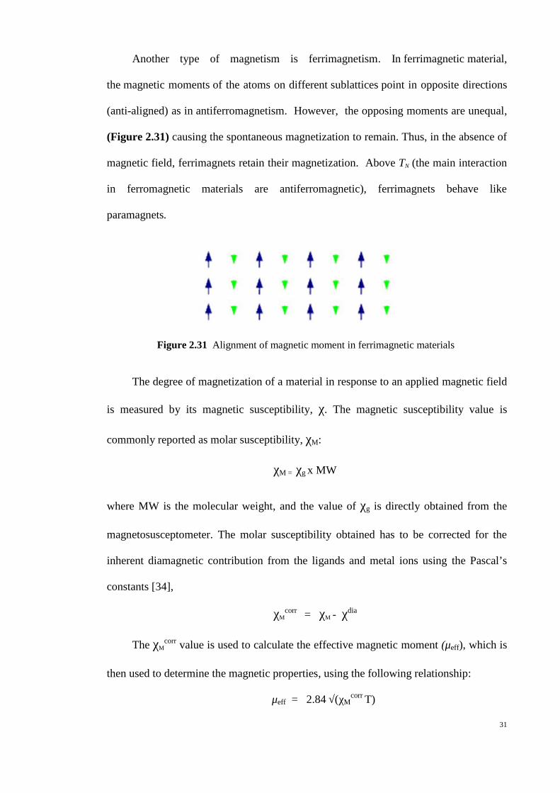
Another type of magnetism is ferrimagnetism. In ferrimagnetic material,

the magnetic moments of the atoms on different sublattices point in opposite directions

(anti-aligned) as in antiferromagnetism. However, the opposing moments are unequal,

(Figure 2.31) causing the spontaneous magnetization to remain. Thus, in the absence of

magnetic field, ferrimagnets retain their magnetization. Above TN (the main interaction

in ferromagnetic materials are antiferromagnetic), ferrimagnets behave like

paramagnets.

The degree of magnetization of a material in response to an applied magnetic field

is measured by its magnetic susceptibility, χ. The magnetic susceptibility value is

commonly reported as molar susceptibility, χM:

χM = χg x MW

where MW is the molecular weight, and the value of χg is directly obtained from the

magnetosusceptometer. The molar susceptibility obtained has to be corrected for the

inherent diamagnetic contribution from the ligands and metal ions using the Pascal’s

constants [34],

χMcorr = χM - χdia

The χMcorr value is used to calculate the effective magnetic moment (μeff), which is

then used to determine the magnetic properties, using the following relationship:

μeff = 2.84 √(χMcorr T)

Figure 2.31 Alignment of magnetic moment in ferrimagnetic materials

32

where T is the absolute temperature (in K). Sometimes, the equation is also presented

as:

μeff = 2.84 (χMcorr T- Nα)½

where Nα is the temperature independence paramagnetism (TIP) of a metal ion. The

value for each copper(II) ion is 60 x 10-6 c.g.s emu.

Theoretically, μeff , may be calculated from the following relationship:

μeff = √n(n+2)

where n is the number of unpaired electron(s).

Copper(II) ion (3d9) has one unpaired electron in the 3d orbitals. Thus, using the

above equation, the calculated μeff value for mononuclear copper(II) complexes (at room

temperature) is expected to be 1.73 B.M., while the value for dinuclear copper(II)

complexes (two unpaired electrons) is 2.83 B.M.

Magnetic moments of copper(II) complexes can be classified into two main

groups: (a) normal moments (1.8 – 2.0 B.M. for one unpaired electron), indicating the

absence of any magnetic interaction between the unpaired electron of each copper(II)

centre; and (b) magnetic moments smaller than the spin only value [35], also known as

subnormal magnetic moments.

Copper(II) complexes with subnormal magnetic moments can be classified based

on the type of mechanisms of magnetic interaction: (a) direct interaction; and (b)

superexchange interaction. The direct copper-to-copper magnetic interaction is due to

the direct bond between the two copper(II) ions, which is illustrated by copper(II)

acetate monohydrate in which Cu-Cu distance is short, 2.64 Ao (μeff =1.43 B.M). For the

second group, the copper-to-copper interaction is through the ligands, termed the super-

exchange interaction [35,36].

33

Another important numerical value when discussing magnetic interaction is the 2J

value (the exchange integral). It corresponds to the separation energy between a singlet

and a triplet state [37]. For a dimeric copper(II) complex, the 2J value is calculated

using the Bleaney-Bowers equation:

χm =

N2)e311(

T3Ng2 1T

J222

This equation is simplified by rearranging the above equation and by putting the

values for all the constants [38]:

-2J = {ln[{1.2186 x 10-2/(χm – 0.12x 10-3)} -3]}207.11

A negative 2J value indicates a singlet ground state and hence an

antiferromagnetic interaction, while a positive 2J value indicates a triplet ground state

and hence a ferromagnetic interaction.

The expected 2J values for copper(II) carboxylates range from

-100 cm-1 to -500 cm-1. The higher (more negative) value indicates a stronger

antiferromagnetic interaction [39,40].

2.11 Cyclic Voltammetry

Cyclic voltammetry (CV) is an electrochemical technique with the objective to study

the redox behaviour of a complex. In CV, the potential of a working electrode is

changed linearly with time, in the potential region where reduction or oxidation of the

material being studied occurs. The direction of the linear sweep is then reversed, and the

electrode reactions are detected. A plot of current at the working electrode versus the

applied voltage gives a cyclic voltammogram.

CV experiments involve a three electrode system: (a) saturated calomel electrode

as the reference electrode; (b) a glassy carbon electrode as the working electrode; and

34

(c) a platinum wire as the counter electrode. Tetrabutylammonium tetrafluoroborate

(TBABF4) of molarity about 10-3 M may be used as the surporting electrolyte to ensure

the required conductive media

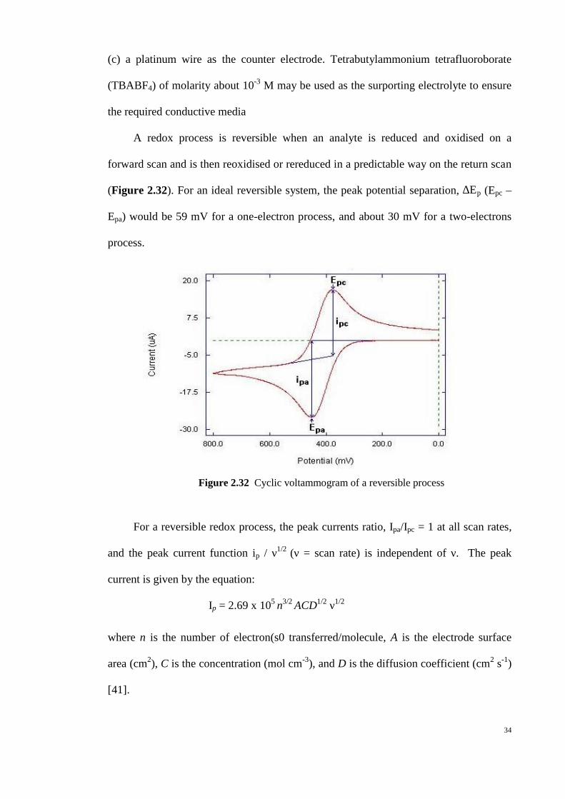
A redox process is reversible when an analyte is reduced and oxidised on a

forward scan and is then reoxidised or rereduced in a predictable way on the return scan

(Figure 2.32). For an ideal reversible system, the peak potential separation, ∆Ep (Epc –

Epa) would be 59 mV for a one-electron process, and about 30 mV for a two-electrons

process.

For a reversible redox process, the peak currents ratio, Ipa/Ipc = 1 at all scan rates,

and the peak current function ip / ν1/2 (ν = scan rate) is independent of ν. The peak

current is given by the equation:

Ip = 2.69 x 105 n3/2 ACD1/2 ν1/2

where n is the number of electron(s0 transferred/molecule, A is the electrode surface

area (cm2), C is the concentration (mol cm-3), and D is the diffusion coefficient (cm2 s-1)

[41].

Figure 2.32 Cyclic voltammogram of a reversible process

35

Variation from the above parameters leads to a quasi-reversible process, which

may be caused by the slow electron transfer kinetics and to the formation of chemical

reaction following the electron transfer. In this case, the return wave could be observed

but with amplitude less than the forward wave. It is characterized by the value of ∆Ep

greater than 59/n mV and the value of Ipa/Ipc of less than unity.

Most dimeric copper(II) carboxylates showed quasi-reversible redox processes

[16,21,24,42] (which occur in a stepwise process) due to the change in the geometry of

the coordination sphere. As one of the Cu(II) ion in the dimer is reduced to Cu(I), some

structural distortion of the dimer took place [42] as Cu(II) ion prefers the square planar

geometry while Cu(I) prefers the tetrahedral geometry.

References

[1] A.M. Giroud-Godquin. Coord. Chem. Rev., 178, 1485 (1998).

[2] R. Giménez, D.P. Lydon, J.L. Serrano. Curr Opin Solid State Mater Sci., 6, 527

(2002).

[3] R.W. Date, E.F. Iglesias, K.E. Rowe, J.M. Elliott, D.W. Bruce. Dalton Trans.,

1914 (2003).

[4] D.W.Bruce, E. Lalinde, P. Styring, D. A. Dunmur and P.M. Maitlis, J. Chem.

Soc., Chem. Commun., 1986, 581; H.Adams, N.A. Bailey, D. W. Bruce, D.A

Dunmur, E. Lalinde, M. Marcos, C. Ridgway, A.J Smith, P. Styring and P.M.

Maitlis, Liq. Cryst., 2, 381 (1987).

[5] K. Ohta, O. Takenaka, H. Hasebe, Y. Morizumi, T. Fujimoto and I. Yamamoto,

Mol. Cryst., Liq. Cryst., 195, 135 (1991).

[6] S. Chandrasekhar, B.K. Sadashiva and K.A. Suresh, Pranama 9, 471-480

(1977).

36

[7] Fabio D. Cukiernik, Mohammed Ibn-Elhaj, Zulema D. Chaia, Jean-Claude

Marchon, Anne-Marie Giroud-Godquin, Daniel Guillon, Antoine Skoulios, and

Pascale Maldivi, Chem. Mater. 10, 83-91 (1998).

[8] Van Niekerk, J. N., and Schoening, F. R. L., Acta Cryst., 6, 227 (1953).

[9] J. A. R. Cheda, M. V. Garcia, M. I. Redondo, S. Gargani and P. Ferloni, Liquid

Crystals, Vol., No., 1, 1-14 (2004).

[10] Tom Welton (Eds.), Coordination Chemistry Review 248 2459-2477 (2004).

[11] Harry D. Pratt III, Alyssa J. Rose, Chad L. Staiger, David Ingersoll and Travis

M, Anderson, Dalton Trans. 40, 11396 (2011).

[12] M. Brett Meredith, C. Heather McMillen, Jonathan T. Goodman and Timothy P.

Hanusa, Polyhedron, 28, 2355-2358 (2009).

[13] Bojan Kozlevcar and Primož Šegedin, Croatica Chemica Acta, CCACAA 81 (2)

369-379 (2008).

[14] http://en.wikipedia.org/wiki/Coordination_compound

[15] Frank P. W. Agterberg, Hajo A. J. Provo Kluit, Willem L. Driessen, Henk

Oevering, Wim Buijs, Miles T. Lakin, Anthony L. Spek and Jan Reedijk, Inorg.

Chem., 36, 4321-4328 (1997).

[16] M. I. Mohamadin, N. Abdullah, Cent. Eur. J. Chem. 8(5), 1090-1096 (2010)

[17] http://en.wikipedia.org/wiki/Aldol_reaction.

[18] B. Adhikary, A. K. Biswas and K. Nag, Polyhedron, 6(6), 3208 (1987).

[19] Pavia, Lampman, Kriz, Introduction to Spectroscopy, 3rd. Edition.

[20] G. B. Deacon, R. J. Philips, Coord. Chem. Rev., 33, 227 (1980).

[21] Angel Garcio-Raso, Juan J. Fiol, Adela Lopez-Zafra, Jose A. Castro, Araceli

Cabrero, Ignasi Mata an Elies Molins, Polyhedron, 22, 403 (2003).

[22] P.Kogerler, P.A.M. Williams, B.S. Parajon-Costa, E.J.Baran, L.Lezama, T.Rojo,

A.Muller, Inorganica Chimica Acta, 268, 239-248 (1998).

37

[23] C. Yenikaya, M. Poyraz, M. Sari, F. Demirci, H. Ilkimen, O. Buyukgungor,

Polyhedron, 28, 3526-3532 (2009).

[24] S. Karthikeyan, T. M. Rajendiran, R. Kannappan, R. Mahalakshmy, R.

Venkatesan and P. Sambasiva Rao, Proc. Indian Acad. Sci. (Chem. Sci.), Vol.

113, No. 4, 245-256 (2001).

[25] K. S. Bharati, S. Sreedaran, A. K. Rahiman, K. Rajesh, V. Narayanan,

Polyhedron, 26, 3993 (2007).

[26] http://en.wikipedia.org/wiki/JahnTeller_effect

[27] A. Garcis-Raso, J.J. Fiol, F. Badenas, E. Lago, E. Mollins, Polyhedron, 20, 2877

(2001).

[28] B. K. Koo. Bull. Korean Chem. Soc., 22(1), 113 (2001).

[29] E. Kokot, R. L. Martin, Inorg. Chem., 3, 1306 (1964).

[30] M. Petric, I. Leban and P. Segedin, Polyhedron Vol. 14, No. 8, pp. 983-989

(1995).

[31] M. Pajtasova, D. Ondrusova, E. Jona, S. C. Jona, S. C. Mojumdar, S. L’alikova,

T. Bazylakova, M. Gregor, J. Therm Anal Calorim 100, 769-777 (2010).

[32] Images for liquid crystals images, york.ac.uk; phys.kent.edu; dept.kent.edu;

sciencewhizkids.blogspot.com; nanohedron.com; mc2.chalmers.se.

[33] J. C. Marchon, P. Maldivi, A. M. Giroud-Godquin, D. Guillon, A. Skoulios and

D. P. Strommen, Phil. Trans. R. Soc. Lond. A 330, 109-116 (1990).

[34] Gordon A. Bain and John F. Berry, Journal of Chemical Education, Vol. 85, No.

4 (2008).

[35] Motomichi Inoue, Michihiko Kishita and Masaji Kubo, Inorg. Chem., Vol. 3,

No. 2, (1964).

[36] Michinobu Kato, Hans B. Jonassen and James C. Fanning, Chem Rev., 64, 99

(1964).

38

[37] Ahyan Elmali, Turk J. Phy., 24, 667-672 (2000).

[38] D.W. Bruce and D O’Hare, Inorganic Materials 2nd Edition, John Wiley and

Sons, New York, p. 70 (1996).

[39] Rocio Cejudo, Gloria Alzuet, Joaquin Borras, Malva Liu-Gonzalez, Francisco

Sanz-Ruiz, Polyhedron, 21, 1057-1061 (2002).

[40] L. Strinna Erre, G. Micera, P.Piu, F. Cariati and G. Ciani, Inorg. Chem. 24,

2297-2300 (1985)

[41] www.basinc.com/mans/EC_epsilon/Techniques/CycVolt/cv_analysis.html.

[42] M. I. Mohamadin and N. Abdullah, International Journal of the Physical

Sciences, Vol. 6(8) (2011).