Chapter 2 Limits and Continuitymathstat.sci.tu.ac.th/~archara/MA111/MA111-118/... · Limits and...
30
Chapter 2 Limits and Continuity 2.1 Limits The limits is the fundamental notion of calculus. This underlying concept is the thread that binds together virtually all of the calculus you are about to study. In this section, we develop the notion of limit using some common language and illustrate the idea with some simple examples. As a start, consider the function f (x)= x 2 − 1 x − 1 and g (x)= x 2 − 2 x − 1 Notice that both functions are undefined at x = 1. But we can examine their behavior for x close to 1, as in the following table. x f (x)= x 2 − 1 x − 1 g (x)= x 2 − 2 x − 1 0.9 1.9 11.9 0.99 1.99 101.99 0.999 1.999 1, 001.999 0.9999 1.9999 10, 001.9999 0.99999 1.99999 100, 001.99999 0.999999 1.999999 10, 000, 001.999999 Notice that as you move down the first column of the table, the x-values get closer to 1, but all less than 1. We use the notation x → 1 - to indicate that x approaches 1 from the left side. Notice that the table suggest that as x gets closer and closer to 1 (with x< 1), f (x) is getting closer and closer to 2. In view of this, we say that the limit of f (x) as x approaches 1 from the left is 2, written lim x→1 - f (x)=2. On the other hand, the table indicate that as x gets closer and closer to 1 (with x< 1), g (x) increases without bound. In this case, g (x) is said to increase without bound as x approaches 1 from the left, written lim x→1 - g (x)=+∞ 3
Transcript of Chapter 2 Limits and Continuitymathstat.sci.tu.ac.th/~archara/MA111/MA111-118/... · Limits and...

Chapter 2
Limits and Continuity
2.1 Limits
The limits is the fundamental notion of calculus. This underlying concept is the threadthat binds together virtually all of the calculus you are about to study.
In this section, we develop the notion of limit using some common language andillustrate the idea with some simple examples.
As a start, consider the function
f(x) =x2 − 1
x− 1and g(x) =
x2 − 2
x− 1
Notice that both functions are undefined at x = 1. But we can examine their behaviorfor x close to 1, as in the following table.
x f(x) =x2 − 1
x− 1g(x) =
x2 − 2
x− 10.9 1.9 11.90.99 1.99 101.990.999 1.999 1, 001.9990.9999 1.9999 10, 001.99990.99999 1.99999 100, 001.999990.999999 1.999999 10, 000, 001.999999
Notice that as you move down the first column of the table, the x-values get closerto 1, but all less than 1. We use the notation x → 1− to indicate that x approaches
1 from the left side. Notice that the table suggest that as x gets closer and closer to1 (with x < 1), f(x) is getting closer and closer to 2. In view of this, we say that thelimit of f(x) as x approaches 1 from the left is 2, written
limx→1−
f(x) = 2.
On the other hand, the table indicate that as x gets closer and closer to 1 (with x < 1),g(x) increases without bound. In this case, g(x) is said to increase without bound asx approaches 1 from the left, written
limx→1−
g(x) = +∞
3
MA111: Prepared by Asst.Prof.Dr. Archara Pacheenburawana 4
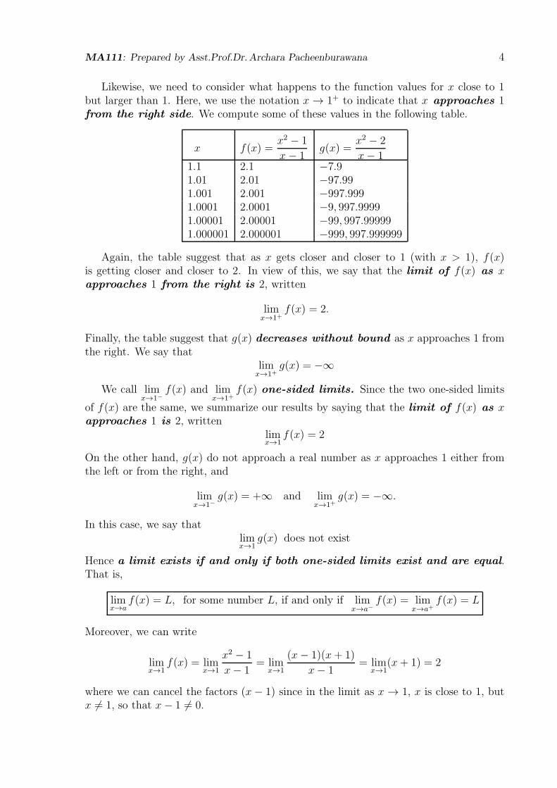
Likewise, we need to consider what happens to the function values for x close to 1but larger than 1. Here, we use the notation x → 1+ to indicate that x approaches 1from the right side. We compute some of these values in the following table.
x f(x) =x2 − 1
x− 1g(x) =
x2 − 2
x− 11.1 2.1 −7.91.01 2.01 −97.991.001 2.001 −997.9991.0001 2.0001 −9, 997.99991.00001 2.00001 −99, 997.999991.000001 2.000001 −999, 997.999999
Again, the table suggest that as x gets closer and closer to 1 (with x > 1), f(x)is getting closer and closer to 2. In view of this, we say that the limit of f(x) as xapproaches 1 from the right is 2, written
limx→1+
f(x) = 2.
Finally, the table suggest that g(x) decreases without bound as x approaches 1 fromthe right. We say that
limx→1+
g(x) = −∞
We call limx→1−
f(x) and limx→1+
f(x) one-sided limits. Since the two one-sided limits
of f(x) are the same, we summarize our results by saying that the limit of f(x) as xapproaches 1 is 2, written
limx→1
f(x) = 2
On the other hand, g(x) do not approach a real number as x approaches 1 either fromthe left or from the right, and
limx→1−
g(x) = +∞ and limx→1+
g(x) = −∞.
In this case, we say thatlimx→1
g(x) does not exist
Hence a limit exists if and only if both one-sided limits exist and are equal.That is,
limx→a
f(x) = L, for some number L, if and only if limx→a−
f(x) = limx→a+
f(x) = L
Moreover, we can write
limx→1
f(x) = limx→1
x2 − 1
x− 1= lim
x→1
(x− 1)(x+ 1)
x− 1= lim
x→1(x+ 1) = 2
where we can cancel the factors (x− 1) since in the limit as x → 1, x is close to 1, butx 6= 1, so that x− 1 6= 0.

MA111: Prepared by Asst.Prof.Dr. Archara Pacheenburawana 5
Determine whether or not limx→0
1
xexists.
Example 2.1.
Solution We first graph y =1
xand compute some function values for x close to 0.
−3 3
10
−10
x
y
y =1
x
x 1/x±0.1 ±10±0.01 ±100±0.001 ±1000±0.0001 ±10, 000±0.00001 ±100, 000
Notice that, as x → 0+,1
xincreases without bound. Thus,
limx→0+
1
x= +∞.
Likewise, we can say that
limx→0−
1
x= −∞.
Therefore,
limx→0
1
xdoes not exist. z
Evaluate limx→0
sin x
x.
Example 2.2.
Solution We graph f(x) =sin x
xand compute some function values.
x
y
y =sinx
x
1
0 1 2 3−1−2−3
x (sin x)/x
±0.1 0.998334±0.01 0.999983±0.001 0.99999983±0.0001 0.9999999983±0.00001 0.999999999983

MA111: Prepared by Asst.Prof.Dr. Archara Pacheenburawana 6
The graph and the tables of value lead us to
limx→0+
sin x
x= 1 and lim
x→0−
sin x
x= 1
Thus,
limx→0
sin x
x= 1. z
1
2
3
4
5
6
−1
−2
−3
1 2 3 4 5 6 7−1−2−3−4
x
y
b bc
b
bc
For the function whose graph is given, state the value of the given quantity, ifit does not exist, explain why.
(a) limx→2−
f(x) = (b) limx→2+
f(x) =
(c) limx→2
f(x) = (d) limx→−1−
f(x) =
(e) limx→−1+
f(x) = (f) limx→−1
f(x) =
Example 2.3.

MA111: Prepared by Asst.Prof.Dr. Archara Pacheenburawana 7
Exercises 2.1
1.
x
y
1
y = f(x)
For the function whose graph is given, state the value of the given quantity, if itdoes not exist, explain why.
(a) limx→0−
f(x) (b) limx→0+
f(x)
(c) limx→0
f(x) (d) limx→2−
f(x)
(e) limx→2+
f(x) (f) limx→2
f(x)
(g) limx→−3
f(x)
2.
-4 -3 -2 -1 0 1 2 3 4 5
-4
-3
-2
-1
0
1
2
3
4 y
x
b
b
y = f(x)
For the function whose graph is given, state the value of the given quantity, if itdoes not exist, explain why.
(a) limx→1
f(x) (b) limx→3−
f(x)
(c) limx→3+
f(x) (d) limx→3
f(x)
(e) f(3) (f) limx→−2−
f(x)
(g) limx→−2+
f(x) (h) limx→−2
f(x)
(i) f(−2)

MA111: Prepared by Asst.Prof.Dr. Archara Pacheenburawana 8
3.
-4 -3 -2 -1 0 1 2 3 4-1
0
1
2
3
4
x
y
bcbc
b
b
b
bc
y = f(x)
For the function whose graph is given, state the value of the given quantity, if itdoes not exist, explain why.
(a) limx→−3
f(x) (b) f(−3)
(c) f(−1) (d) limx→−1
f(x)
(e) f(1) (f) limx→1−
f(x)
(g) limx→1+
f(x) (h) limx→1
f(x)
Answer to Exercises 2.1
1. (a) −2 (b) 2 (c) Does not exist (d) −1 (e) 3 (f) Does not exist (g) 2
2. (a) 3 (b) 2 (c) −2 (d) Does not exist (e) 1 (f) −1 (g) −1 (h) −1 (i) −3
3. (a) 2 (b) 1 (c) 2 (d) 5
2(e) 2 (f) 2 (g) 1 (h) Does not exist
2.2 Computing Limits
In this section we will discuss techniques for computing limits of many functions. Westart with the following basic results.
Let a and k be real numbers.
(a) limx→a
k = k (b) limx→a
x = a (c) limx→0−
1
x= −∞ (d) lim
x→0+
1
x= +∞
Theorem 2.1.
The following theorem will be our basic tool for finding limits algebraically.

MA111: Prepared by Asst.Prof.Dr. Archara Pacheenburawana 9
Let a and k be real numbers. Suppose that limx→a
f(x) = L1 and limx→a
g(x) = L2
Then:
(a) limx→a
[
kf(x)]
= k limx→a
f(x) = kL1
(b) limx→a
[
f(x) + g(x)]
= limx→a
f(x) + limx→a
g(x) = L1 + L2
(c) limx→a
[
f(x)− g(x)]
= limx→a
f(x)− limx→a
g(x) = L1 − L2
(d) limx→a
[
f(x) · g(x)]
= limx→a
f(x) · limx→a
g(x) = L1L2
(e) limx→a
f(x)
g(x)=
limx→a
f(x)
limx→a
g(x)=
L1
L2
, provided L2 6= 0
(f) limx→a
[
f(x)]n
=[
limx→a
f(x)]n
= Ln1 , n a positive integer
(g) limx→a
n
√
f(x) = n
√
limx→a
f(x) = n
√
L1, provided L1 > 0 if n is even.
Moreover, these statements are also true for the one-sided limits as x → a− oras x → a+.
Theorem 2.2 (Limit Laws).
Apply the rules of limits to evaluate the following.
(a) limx→2
(x3 + 4x2 − 3) (b) limx→3
x4 + x2 − 1
x2 + 5(c) lim
x→5
3√3x2 − 4x+ 9
Example 2.4.
Solution

MA111: Prepared by Asst.Prof.Dr. Archara Pacheenburawana 10
For any polynomial
p(x) = cnxn + cn−1x
n−1 + · · ·+ c1x+ c0
and any real number a,
limx→a
p(x) = cnan + cn−1a
n−1 + · · ·+ c1a+ c0 = p(a)
Theorem 2.3 (Limits of Polynomials).
Let f(x) =p(x)
q(x)be the rational function, and let a be any real number.
(a) If q(a) 6= 0, then limx→a
f(x) = f(a).
(b) If q(a) = 0 but p(a) 6= 0, then limx→a
f(x) does not exist.
Theorem 2.4 (Limits of Rational Functions).
Evaluate limx→2
5x3 + 2x− 5
x2 − 3.
Example 2.5.
Solution
Evaluate limx→1
3x2 − x− 2
2x2 + x− 3.
Example 2.6.
Solution

MA111: Prepared by Asst.Prof.Dr. Archara Pacheenburawana 11
Evaluate limx→1
(
1
x− 1− 2
x2 − 1
)
.
Example 2.7.
Solution
Evaluate limx→−3−
|x+ 3|x3 + x2 − 6x
.
Example 2.8.
Solution
Evaluate limx→2
x2/3 − 41/3
x− 2.
Example 2.9.
Solution

MA111: Prepared by Asst.Prof.Dr. Archara Pacheenburawana 12
Evaluate limx→4
x2 − 5x+ 4√x− 2
.
Example 2.10.
Solution
Evaluate limx→3
√x+ 1− 2
x3 − 27.
Example 2.11.
Solution

MA111: Prepared by Asst.Prof.Dr. Archara Pacheenburawana 13
Evaluate limx→2
2− 3√x+ 6
x− 2.
Example 2.12.
Solution
For functions that are defined piecewise, a two-sided limit at a point where theformula for the function changes is best obtained by first finding the one-sided limits atthe point.
Evaluate limx→2
f(x), where f is defined by
f(x) =
x2 − 5x+ 6
|x− 2| for x < 2
2x− 1
x+ 1for x ≥ 2
Example 2.13.
Solution

MA111: Prepared by Asst.Prof.Dr. Archara Pacheenburawana 14
Suppose that g(x) ≤ f(x) ≤ h(x) for all x in some interval (c, d), except possiblyat the point a ∈ (c, d) and that
limx→a
g(x) = limx→a
h(x) = L
for some number L. Then, it follows that
limx→a
f(x) = L.
0 a x
L
y
g
f
h
Theorem 2.5 (The Squeeze Theorem).
The Squeeze Theorem is also called the Sandwich Theorem or the Pinching Theo-rem.
Evaluate limx→1
f(x) if 8 + 2x− x2 ≤ f(x) ≤ 4x+ 5 for all x ∈ R.
Example 2.14.
Solution
Determine the value of limx→0
[
x cos
(
50π
x
)]
.
Example 2.15.
Solution

MA111: Prepared by Asst.Prof.Dr. Archara Pacheenburawana 15
Exercise 2.2
1. Given thatlimx→a
f(x) = −3, limx→a
g(x) = 0, limx→a
h(x) = 8
find the limits that exist. If the limit does not exist, explain why.
(a) limx→a
[
f(x) + h(x)]
(b) limx→a
[
f(x)]2
(c) limx→a
3√
h(x) (d) limx→a
1
f(x)
(e) limx→a
f(x)
h(x)(f) lim
x→a
g(x)
f(x)
(g) limx→a
f(x)
g(x)(h) lim
x→a
2f(x)
h(x)− f(x)
2. Evaluate the following limits.
(a) limx→0
(x2 − 3x+ 1) (b) limx→3
(x3 + 2)(x2 − 5x)
(c) limx→2
x− 5
x2 + 4(d) lim
x→1
(
x4 + x2 − 6
x4 + 2x+ 3
)2
(e) limx→1
√x2 + 2x+ 4 (f) lim
x→4−
√16− x2
(g) limx→−3
x2 − x− 12
x+ 3(h) lim
x→−2
x+ 2
x2 − x− 6
(i) limx→1
x2 + x− 2
x2 − 3x+ 2(j) lim
x→1
x3 − 1
x2 − 1
(k) limh→0
(1 + h)4 − 1
h(l) lim
h→0
(2 + h)3 − 8
h
(m) limt→1
t− 1√t− 1
(n) limt→9
9− t
3−√t
(o) limt→2
t2 + t− 6
t2 − 4(p) lim
t→0
√2− t−
√2
t
(q) limx→2
x4 − 16
x− 2(r) lim
x→9
x2 − 81√x− 3
(s) limx→1
[
1
x− 1− 2
x2 − 1
]
(t) limt→0
[
1
t√1 + t
− 1
t
]
(u) limh→0
(3 + h)−1 − 3−1
h(v) lim
x→2
1
x− 1
2
x− 2
(w) limx→1
√x− x
1−√x
(x) limx→0
x√1 + 3x− 1
(y) limx→0
√3 + x−
√3
x(z) lim
x→0
xe−2x+1
x2 + 1
3. Evaluate limx→2
f(x) where f(x) =
{
3x2 − 2x+ 1 if x < 2x3 + 1 if x ≥ 2

MA111: Prepared by Asst.Prof.Dr. Archara Pacheenburawana 16
4. Evaluate limx→2
f(x) where f(x) =
{
2x if x < 2x2 if x ≥ 2
5. Evaluate limx→0
f(x) where f(x) =
{
x2 + 1 if x < −13x+ 1 if x ≥ −1
6. Evaluate limx→−1
f(x) where f(x) =
2x+ 1 if x < −13 if −1 ≤ x < 12x+ 1 if x ≥ 1
7. Find the limit, if it exists. If the limit does not exist, explain why.
(a) limx→−4
|x+ 4| (b) limx→−4−
|x+ 4|x+ 4
(c) limx→1.5
2x2 − 3x
|2x− 3| (d) limx→0+
(
1
x− 1
|x|
)
8. Use the Squeeze Theorem to find the following limits.
(a) limx→0
x2 sin(1/x)
(b) limx→0
x2 cos(20πx)
(c) limx→0
√x3 + x2 sin
π
x
Answer to Exercise 2.2
1. (a) 5 (b) 9 (c) 2 (d) −1
3(e) −3
8(f) 0 (g) −∞ (h) − 6
11
2. (a) 1 (b) −174 (c) −3
8(d) 4
9(e)
√7 (f) 0 (g) −7 (h) −1
5(i) −3
(j) 3
2(k) 4 (l) 12 (m) 2 (n) 6 (o) 5
4(p) −
√2
4(q) 32 (r) 108 (s) 1
2
(t) −1
2(u) −1
9(v) −1
4(w) 1 (x) 2
3(y) 1
2√3
(z) 0
3. 9 4. 4 5. 1 6. Does not exist 7. (a) 0 (b) −1 (c) Does not exist (d) 0
8. (a) 0 (b) 0 (c) 0

MA111: Prepared by Asst.Prof.Dr. Archara Pacheenburawana 17
2.3 Limits at Infinity
Let’s begin by investigating the behavior of the function f defined by
f(x) =x2 − 1
x2 + 1
as x becomes large.
x
y
y = 1
x f(x) =x2 − 1
x2 + 1
±0 −1±1 0±2 0.600000±3 0.800000±4 0.882353±5 0.923077±10 0.980198±50 0.999200±100 0.999800±1000 0.999998
As x grows larger and larger we can see from the graph and the table of values thatthe values of f(x) get closer and closer to 1. That is,
limx→∞
x2 − 1
x2 + 1= 1.
In general, we use the notationlimx→∞
f(x) = L
indicates that the values of f(x) becomes closer and closer to L as x becomes larger andlarger.
Let f be a function defined on some interval (a,∞). Then
limx→∞
f(x) = L
mean that the value of f(x) can be made arbitrarily close to L by taking xsufficiently large.
Definition 2.1.
Referring back to the above Figure, we see that for numerically large negative valuesof x, the values of f(x) are close to 1, that is,
limx→−∞
x2 − 1
x2 + 1= 1.
The general definition is as follows.

MA111: Prepared by Asst.Prof.Dr. Archara Pacheenburawana 18
Let f be a function defined on some interval (−∞, a). Then
limx→−∞
f(x) = L
mean that the value of f(x) can be made arbitrarily close to L by taking xsufficiently large negative.
Definition 2.2.
The line y = L is called a horizontal asymptote of the curve y = f(x) ifeither
limx→∞
f(x) = L or limx→−∞
f(x) = L
Definition 2.3.
For instance, the curve illustrated in Figure above has the line y = 1 as a horizontalasymptote because
limx→∞
x2 − 1
x2 + 1= 1.
For any rational number t > 0,
limx→±∞
1
xt= 0
where for the case where x → −∞, we assume that t =p
qwhere q is odd.
Theorem 2.6.
For a polynomial of degree n > 0,
pn(x) = anxn + an−1x
n−1 + · · ·+ a1x+ a0,
we have
limx→∞
pn(x) =
{
∞, if an > 0−∞, if an < 0
Theorem 2.7.

MA111: Prepared by Asst.Prof.Dr. Archara Pacheenburawana 19
Evaluate limx→∞
x3 − 2x+ 4
3x2 + 3x− 5.
Example 2.16.
Solution
Evaluate limx→∞
√x4 − 3x2 + 5
2x2 − x.
Example 2.17.
Solution
Evaluate limx→∞
(√x2 + 3x− x
)
.
Example 2.18.
Solution

MA111: Prepared by Asst.Prof.Dr. Archara Pacheenburawana 20
Evaluate limx→−∞
x3 − 5√x6 − 1− 2x3
.
Example 2.19.
Solution
Exercise 2.3
1− 22 Evaluate the limit, if it exists.
1. limx→∞
x+ 4
x2 − 2x+ 52. lim
x→−∞
(1− x)(2 + x)
(1 + 2x)(2− 3x)
3. limx→−∞
−x√4 + x2
4. limx→−∞
x3 − 2x+ 1
3x3 + 4x− 1
5. limx→∞
x3 − 2x+ 4
3x2 + 3x− 56. lim
x→∞
x2 − sin x
x2 + 4x− 1
7. limx→∞
3x3 − x+ 5
4x3 + 4x2 − 18. lim
x→∞
x4 − x2 + 1
x5 + x3 − x
9. limx→∞
(√x2 + 3− x
)
10. limx→∞
√x2 + 4x
4x+ 1
11. limx→∞
1−√x
1 +√x
12. limx→∞
(√x2 + 1−
√x2 − 1
)
13. limx→∞
(√9x2 + x− 3x
)
14. limx→∞
√x
15. limx→∞
(
x−√x)
16. limx→−∞
(x3 − 5x2)
17. limx→∞
x7 − 1
x6 + 118. lim
x→∞e2x
19. limx→∞
sin 2x 20. limx→∞
e−3x cos 2x
21. limx→∞
ln(2x) 22. limx→0+
(x ln 2x)
23. limx→−∞
x3 − 5√x6 − 1− 2x3
24. limx→−∞
x3 − 1
x3 −√x6 − 1

MA111: Prepared by Asst.Prof.Dr. Archara Pacheenburawana 21
25− 30 Find the horizontal asymptotes of each curve, if it exists.
25. f(x) =x
x+ 426. f(x) =
x√4 + x2
27. f(x) =x
4− x228. f(x) =
x3
4− x2
29. f(x) =x3
x2 + 3x− 1030. f(x) =
x4√x4 + 1
Answer to Exercise 2.3
1. 0 2. 1
63. 1 4. 1
35. ∞ 6. 1 7. 3
48. 0 9. 0 10. 1
411. −1 12. 0
13. 1
614. ∞ 15. ∞ 16. −∞ 17. ∞ 18. ∞ 19. Does not exist 20. 0
21. ∞ 22. 0 23. 1
324. 1
225. y = 1 26. y = −1, y = 1 27. y = 0
28. No horizontal asymptote 29. No horizontal asymptote 30. y = −1, y = 1
2.4 Limit of Trigonometric Functions
limx→0
sin x = 0
Lemma 2.1.
limx→0
sin x
x= 1
Lemma 2.2.
For any real number k 6= 0,
limx→0
sin kx
x= k
Corollary 2.1.
Evaluate limx→0
1− cos 2x
x2.
Example 2.20.
Solution

MA111: Prepared by Asst.Prof.Dr. Archara Pacheenburawana 22
Evaluate limx→0+
2x− sin x
tan 2x.
Example 2.21.
Solution
Evaluate limx→0
2x cot2 x
csc x.
Example 2.22.
Solution
Evaluate limx→0
1− cosx
x sin x.
Example 2.23.
Solution

MA111: Prepared by Asst.Prof.Dr. Archara Pacheenburawana 23
Exercise 2.4
1− 10 Evaluate the limits.
1. limx→0
sin 5x
3x2. lim
t→0
sin 8t
sin 9t
3. limθ→0
cos θ − 1
sin θ4. lim
x→0
sin2 x
x
5. limx→0
tan x
4x6. lim
x→0
cot 2x
csc x
7. limx→π/4
sin x− cosx
cos 2x8. lim
x→0
2x cot2 x
csc x
9. limx→0
x+ sin x
tan x10. lim
x→0
sin(cosx)
sec x
11. limx→0
1− cos x
x sin x
Answer to Exercise 2.4
1. 5
32. 8
93. 0 4. 0 5. 1
46. 1
27. − 1√
28. 2 9. 2 10. sin 1 11. 1
2
2.5 Continuity
It is helpful for us to first try to see what it is about the function whose graphs areshown below that makes them discontinuous at the point x = a.
x
y
ax
y
b
ax
y
a
This suggests the following definition of continuity at a point.
A function f is continuous at x = a when
(i) f(a) is defined,
(ii) limx→a
f(x) exists and
(iii) limx→a
f(x) = f(a).
Otherwise, f is said to be discontinuous at x = a.
Definition 2.4.

MA111: Prepared by Asst.Prof.Dr. Archara Pacheenburawana 24
From the graph of f , state the numbers at which f is discontinuous and explainwhy.
x
y
b
0 1 3 5
Example 2.24.
Solution
Where are each of the following functions discontinuous?
(a) f(x) =x5 − 3x2 + 5
x2 − 3x+ 2
(b) g(x) =
2x2 − 5x− 3
x− 3if x 6= 3
6 if x = 3
Example 2.25.
Solution

MA111: Prepared by Asst.Prof.Dr. Archara Pacheenburawana 25
For what value of a is
f(x) =
{
x2 − 1 if x < 32ax if x ≥ 3
continuous at every x.
Example 2.26.
Solution
Let
f(x) =
(x− 2)2
x2 − 4+ 2k if x > 2
h if x = 2
2x+ k if x < 2
Find the values h and k so that f is continuous at x = 2.
Example 2.27.
Solution

MA111: Prepared by Asst.Prof.Dr. Archara Pacheenburawana 26
A function f is right-continuous at a if
limx→a+
f(x) = f(a)
and f is left-continuous at a if
limx→a−
f(x) = f(a).
Definition 2.5.
A function f is is said to continuous on a closed interval [a, b] if the followingconditions are satisfied:
1. f is continuous on (a, b).
2. f is right-continuous at a.
3. f is left-continuous at b.
Definition 2.6.
Show that the functionf(x) = x
√16− x2
is continuous on the interval [−4, 4].
Example 2.28.
Solution If −4 < a < 4, then using the Limit Laws, we have
limx→a
f(x) = limx→a
x√16− x2
=(
limx→a
x)(
limx→a
√16− x2
)
=(
limx→a
x)
(
√
limx→a
(16− x2)
)
= a√16− a2 = f(a)
Thus, f is continuous at a if −4 < a < 4. Similar calculations show that
limx→−4+
f(x) = 0 = f(−4) and limx→4−
f(x) = 0 = f(4)
Therefore f is continuous on [−4, 4]. z
MA111: Prepared by Asst.Prof.Dr. Archara Pacheenburawana 27
If f and g are continuous at x = a and c is a constant, then the followingfunctions are also continuous at x = a:
(a) f + g (b) f − g (c) cf
(d) f · g (e)f
g, provided g(a) 6= 0 (f) fn, n a positive integer
Theorem 2.8.
The following types of functions are continuous at every number in their domains:
• polynomials
• rational functions
• root functions
• trigonometric functions
• inverse trigonometric functions
• exponential functions
• logarithmic functions
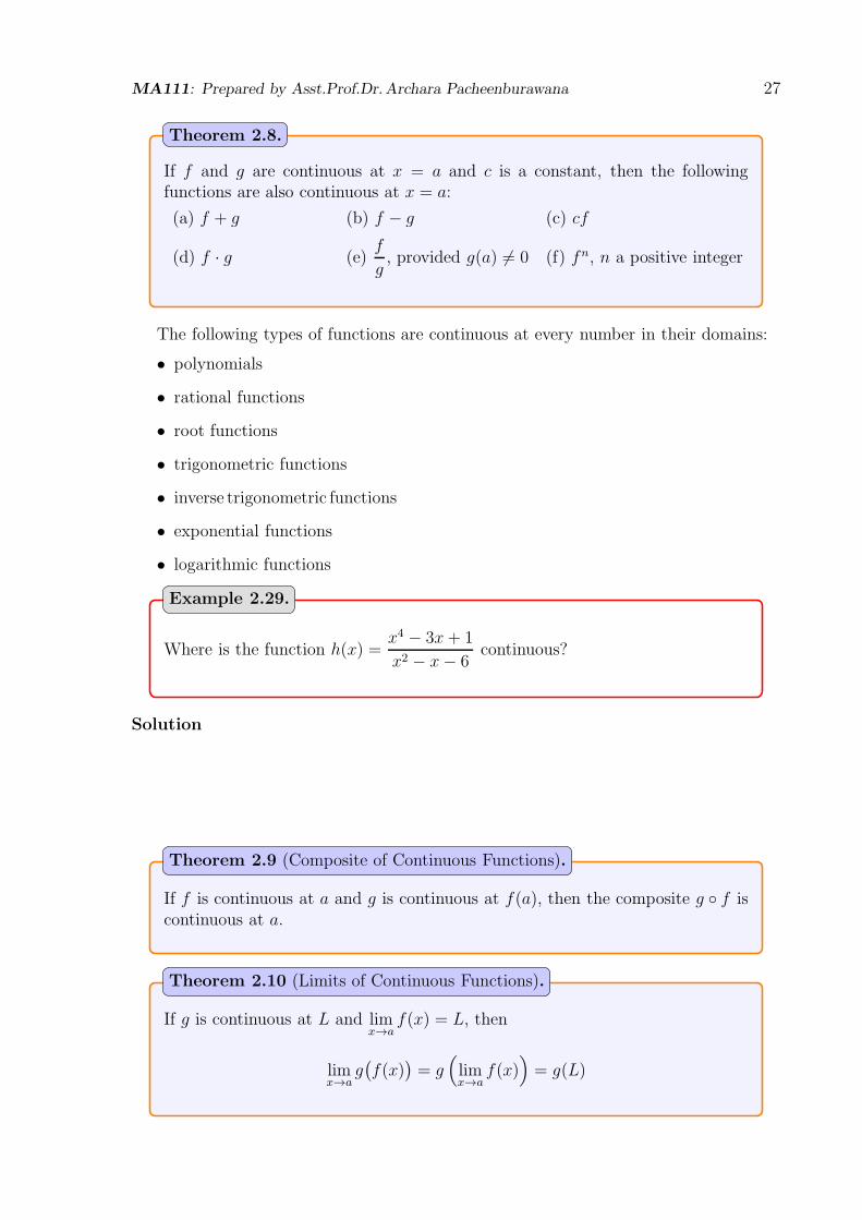
Where is the function h(x) =x4 − 3x+ 1
x2 − x− 6continuous?
Example 2.29.
Solution
If f is continuous at a and g is continuous at f(a), then the composite g ◦ f iscontinuous at a.
Theorem 2.9 (Composite of Continuous Functions).
If g is continuous at L and limx→a
f(x) = L, then
limx→a
g(
f(x))
= g(
limx→a
f(x))
= g(L)
Theorem 2.10 (Limits of Continuous Functions).

MA111: Prepared by Asst.Prof.Dr. Archara Pacheenburawana 28
Evaluate limx→π/2
cos
(
2x+ sin
(
3π
2+ x
))
.
Example 2.30.
Solution
Suppose that f is continuous on the closed interval [a, b] and let N be anynumber between f(a) and f(b). Then there exists a number c ∈ (a, b) such thatf(c) = N .
Theorem 2.11 (Intermediate Value Theorem).
f(a)
N
f(b)
y
a c bx
y = f(x)
(a)
f(a)
N
f(b)
y
a c1 c2 c3 bx
y = f(x)
(b)
Note that the value N can be taken on once [as in part (a)] or more that once [as inpart (b)].
Suppose that f is continuous on [a, b] and f(a) and f(b) have opposite signs.Then, there is at least one number c ∈ (a, b) for which f(c) = 0.
Corollary 2.2.

MA111: Prepared by Asst.Prof.Dr. Archara Pacheenburawana 29
Show that there is a root of the equation x3 − x− 1 = 0 between 1 and 2.
Example 2.31.
Solution Let f(x) = x3 − x − 1. We are looking for a solution of the given equation,that is, a number c between 1 and 2 such that f(c) = 0. Therefore, we take a = 1 andb = 2. We have
f(1) = 13 − 1− 1 = −1 < 0 and f(2) = 23 − 2− 1 = 5 > 0.
Thus f(1) and f(2) have opposite signs. Now f is continuous since it is a polynomial, sothere is a number c ∈ (1, 2) such that f(c) = 0. In other words, the equation x3−x−1 = 0has at least one root c in the interval (1, 2). z
Exercise 2.5
1. Use the given graph to identify all discontinuility of the functions.
(a)
x
y
(b)
x
y
(c)
x
y

MA111: Prepared by Asst.Prof.Dr. Archara Pacheenburawana 30
2. Use the definition of continuity and the properties of limits to show that the func-tion is continuous at the given number.
(a) f(x) = x2 +√7− x , x = 4
(b) g(x) = (x+ 2x3)4, x = −1
(c) h(x) =x+ 1
2x2 + 1, x = 4
3. Use the definition of continuity and the properties of limits to show that the func-tion is continuous on the given interval.
(a) f(x) =1
x+ 1, (−1,∞)
(b) f(x) =x− 1
x2 − 4, (−2, 2)
(c) g(t) =√9− 4t2 , [−3
2, 3
2]
(d) h(z) =√
(z − 1)(3− z) , [1, 3]
4. Explain why the function is discontinuous at the given number.
(a) f(x) =x
x− 1; x = 1
(b) f(x) = sin1
x; x = 0
(c) f(x) = e1/x ; x = 0
(d) f(x) = ln |x− 2| ; x = 2
(e) f(x) =
{ 1
x− 1if x 6= 1
2 if x = 1; x = 1
(f) f(x) =x2 − 1
x+ 1; x = −1
(g) f(x) =
x2 − 2x− 8
x− 4if x 6= 4
3 if x = 4; x = 4
(h) f(x) =
{
1− x if x ≤ 2x2 − 2x if x > 2
; x = 2
(i) f(x) =
x2 if x < 23 if x = 23x− 2 if x > 2
; x = 2
(j) f(x) =
x2 if x < 0−x if 0 ≤ x ≤ 1x if x > 1
; x = 1

MA111: Prepared by Asst.Prof.Dr. Archara Pacheenburawana 31
5. Determine the intervals on which f(x) is continuous.
(a) f(x) = 2x+ 3√x (b) f(x) =
1
x+ 3
(c) f(x) =1
x2 + 1(d) f(x) =
x− 5
|x− 5|
(e) f(x) =x2 + 4
x− 2(f) f(x) = 3
√
x+ 1
x− 1
(g) f(x) =3
x2 − x(h) f(x) =
x
4− x2
(i) f(x) =sin x
x2
6. Find the constant c that makes f(x) continuous on (−∞,∞).
(a) f(x) =
{
x+ c if x < 04− x2 if x ≥ 0
(b) f(x) =
{
c2 − x2 if x < 02(x− c)2 if x ≥ 0
(c) f(x) =
{
cx+ 1 if x ≤ 3cx2 − 1 if x > 3
(d) f(x) =
{
x2 − c2 if x < 4cx+ 20 if x ≥ 4
7. For what value of the constant k is the function
f(x) =
x2 − 2x− 3
|x− 3| ; −2 < x < 3
1− kx√x+ 1
; x ≥ 3
continuous on (−2,∞).
8. For what value of the constant k is the function
f(x) =
x3 + 27
x+ 3if x < −3
(x2 − kx)3 if x ≥ −3
continuous on (−∞,∞).
9. Find the values a and b so that f is continuous on (−∞,∞).
f(x) =
x+ 1 if x < 1ax+ b if 1 ≤ x < 23x+ 1 if x ≥ 2

MA111: Prepared by Asst.Prof.Dr. Archara Pacheenburawana 32
10. Let
f(x) =
{
x2, x 6= 04, x = 0
and g(x) = 2x.
Show thatlimx→0
f(
g(x))
6= f(
limx→0
g(x))
.
11. Use the Intermediate Value Theorem to verify that f(x) has a zero in the giveninterval.
(a) f(x) = x2 − 7 ; [2, 3]
(b) f(x) = x3 − 4x− 2 ; [−1, 0]
(c) f(x) = cosx− x ; [0, 1]
12. Use the Intermediate Value Theorem to show that x3 + 3x− 2 = 0 has a real rootbetween 0 and 1.
13. Use the Intermediate Value Theorem to show that (cos t) t3 + 6 sin5 t − 3 = 0 hasa real root between 0 and 2π.
14. Show that the equation x5 + 4x3 − 7x+ 14 = 0 has at least one real root.
Answer to Exercise 2.5
1. (a) x = −2, 2 (b) x = −2, 1, 4 (c) x = −2, 2, 4
4. (a) f(1) is not defined (b) f(0) is not defined (c) f(0) is not defined
(d) f(2) is not defined (e) limx→1
f(x) is not defined (f) f(−1) is not defined
(g) limx→4
f(x) 6= f(4) (h) limx→2
f(x) is not defined (i) limx→2
f(x) 6= f(2)
(j) limx→1
f(x) is not defined
5. (a) R (b) (−∞,−3)∪(−3,∞) (c) R (d) (−∞, 5)∪(5,∞) (e) (−∞, 2)∪(2,∞)
(f) (−∞, 1)∪(1,∞) (g) (−∞, 0)∪(0, 1)∪(1,∞) (h) (−∞,−2)∪(−2, 2)∪(2,∞)
(i) (−∞, 0) ∪ (0,∞)
6. (a) 4 (b) 0 (c) 1
3(d) −2 7. 3 8. −2 9. a = 5, b = −3