CHAPTER 2 INTRODUCTION TO DNA COMPUTING -...
33
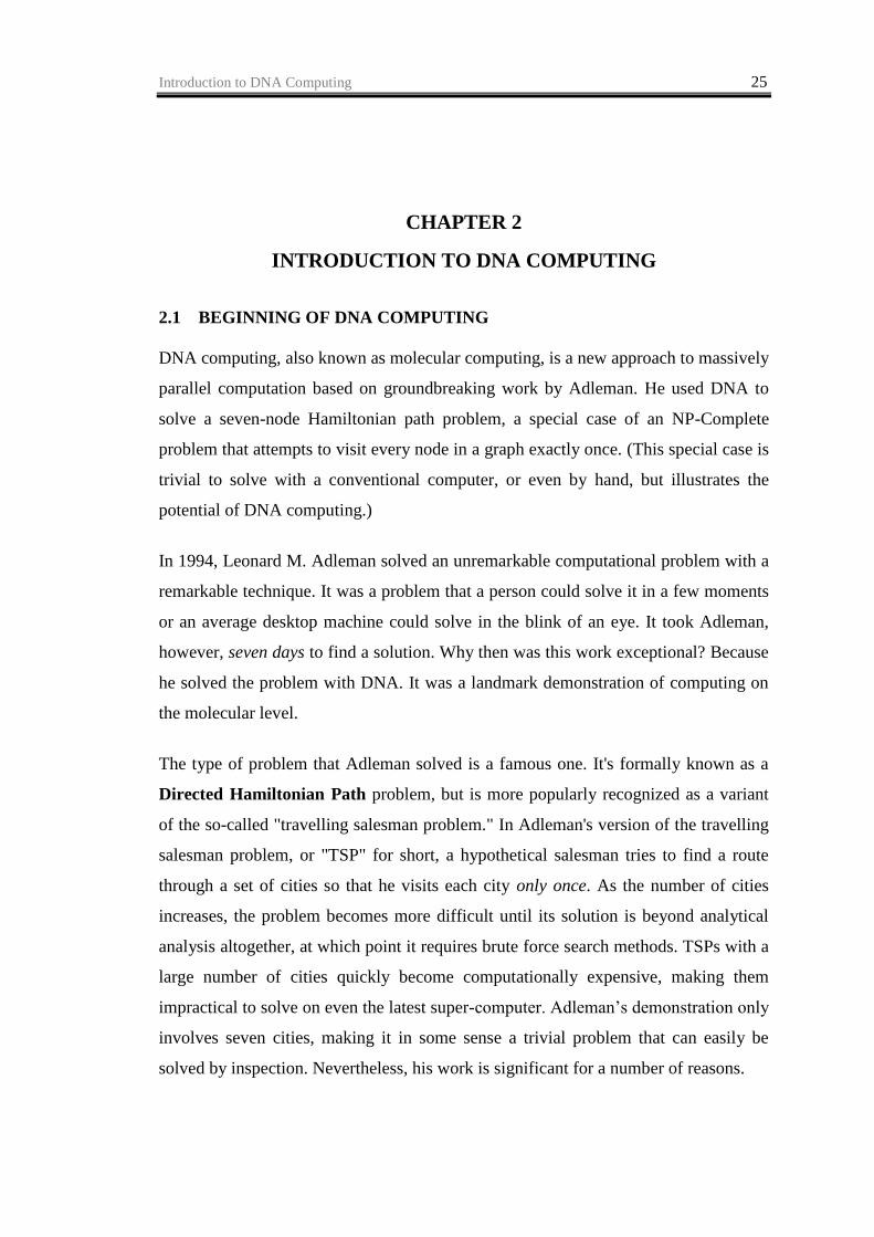
Introduction to DNA Computing 25 CHAPTER 2 INTRODUCTION TO DNA COMPUTING 2.1 BEGINNING OF DNA COMPUTING DNA computing, also known as molecular computing, is a new approach to massively parallel computation based on groundbreaking work by Adleman. He used DNA to solve a seven-node Hamiltonian path problem, a special case of an NP-Complete problem that attempts to visit every node in a graph exactly once. (This special case is trivial to solve with a conventional computer, or even by hand, but illustrates the potential of DNA computing.) In 1994, Leonard M. Adleman solved an unremarkable computational problem with a remarkable technique. It was a problem that a person could solve it in a few moments or an average desktop machine could solve in the blink of an eye. It took Adleman, however, seven days to find a solution. Why then was this work exceptional? Because he solved the problem with DNA. It was a landmark demonstration of computing on the molecular level. The type of problem that Adleman solved is a famous one. It's formally known as a Directed Hamiltonian Path problem, but is more popularly recognized as a variant of the so-called "travelling salesman problem." In Adleman's version of the travelling salesman problem, or "TSP" for short, a hypothetical salesman tries to find a route through a set of cities so that he visits each city only once. As the number of cities increases, the problem becomes more difficult until its solution is beyond analytical analysis altogether, at which point it requires brute force search methods. TSPs with a large number of cities quickly become computationally expensive, making them impractical to solve on even the latest super-computer. Adleman‘s demonstration only involves seven cities, making it in some sense a trivial problem that can easily be solved by inspection. Nevertheless, his work is significant for a number of reasons.
Transcript of CHAPTER 2 INTRODUCTION TO DNA COMPUTING -...
Introduction to DNA Computing 25
CHAPTER 2
INTRODUCTION TO DNA COMPUTING
2.1 BEGINNING OF DNA COMPUTING
DNA computing, also known as molecular computing, is a new approach to massively
parallel computation based on groundbreaking work by Adleman. He used DNA to
solve a seven-node Hamiltonian path problem, a special case of an NP-Complete
problem that attempts to visit every node in a graph exactly once. (This special case is
trivial to solve with a conventional computer, or even by hand, but illustrates the
potential of DNA computing.)
In 1994, Leonard M. Adleman solved an unremarkable computational problem with a
remarkable technique. It was a problem that a person could solve it in a few moments
or an average desktop machine could solve in the blink of an eye. It took Adleman,
however, seven days to find a solution. Why then was this work exceptional? Because
he solved the problem with DNA. It was a landmark demonstration of computing on
the molecular level.
The type of problem that Adleman solved is a famous one. It's formally known as a
Directed Hamiltonian Path problem, but is more popularly recognized as a variant
of the so-called "travelling salesman problem." In Adleman's version of the travelling
salesman problem, or "TSP" for short, a hypothetical salesman tries to find a route
through a set of cities so that he visits each city only once. As the number of cities
increases, the problem becomes more difficult until its solution is beyond analytical
analysis altogether, at which point it requires brute force search methods. TSPs with a
large number of cities quickly become computationally expensive, making them
impractical to solve on even the latest super-computer. Adleman‘s demonstration only
involves seven cities, making it in some sense a trivial problem that can easily be
solved by inspection. Nevertheless, his work is significant for a number of reasons.
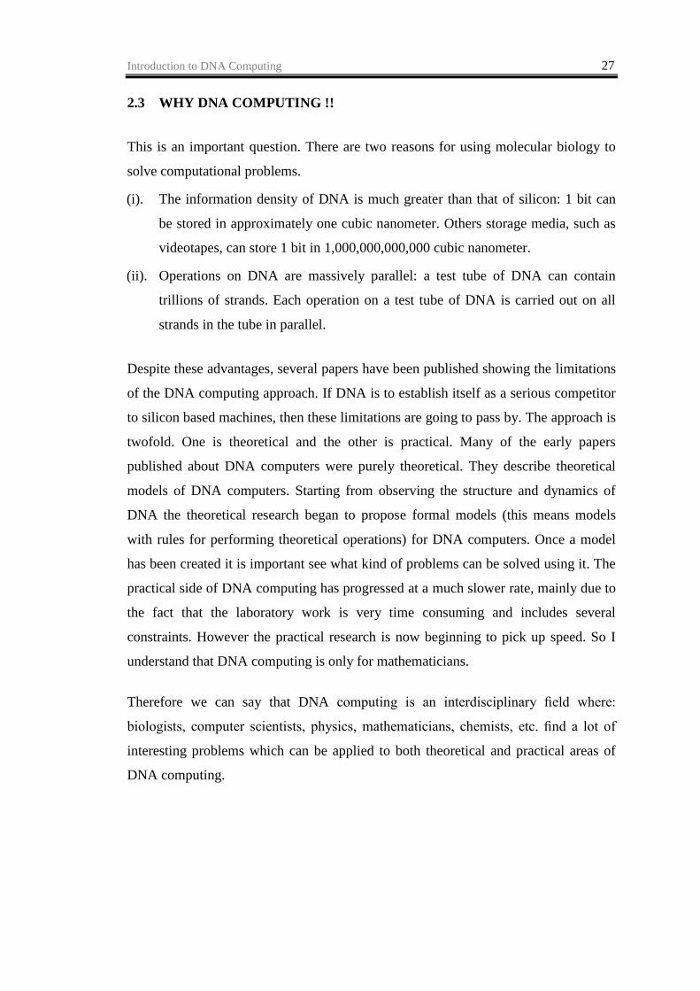
Introduction to DNA Computing 26
It illustrates the possibilities of using DNA to solve a class of problems that is
difficult or impossible to solve using traditional computing methods.
It's an example of computation at a molecular level, potentially a size limit that
may never be reached by the semiconductor industry.
It demonstrates unique aspects of DNA as a data structure
It demonstrates that computing with DNA can work in a massively parallel
fashion.
2.2 CONCEPTS OF DNA COMPUTING AND DNA COMPUTER
A DNA computer is basically a collection of specially selected DNA strands whose
combinations will result in the solution to some problem, depending on the problem at
hand. Technology is currently available both to select the initial strands and to filter
the final solution. The promise of DNA computing is massive parallelism: with a
given setup and enough DNA, one can potentially solve huge problems by parallel
search. This can be much faster than a conventional computer, for which massive
parallelism would require large amounts of hardware, not simply more DNA. Since
Adelman‘s original experiment researchers have developed several different models
to solve other mathematical and computational problems using molecular techniques.
In case of Lipton also, who showed that formula SAT can be solved on a DNA
computer generalized Adleman‘s techniques. These algorithms essentially use a brute
force approach to solve hard combinatorial problems. This approach is interesting due
to the massive parallelism available in DNA computers. Also there are class of
algorithms which can be implemented on a DNA computer, namely some algorithms
based on dynamic programming. Graph connectivity and knapsack are classical
problems solvable in this way. These problems are solvable by conventional
computers in polynomial time, but only so long as they are small enough to fit in
memory. DNA computers using dynamic programming could solve substantially
larger instances because their large memory capacity than either conventional
computers or previous brute force algorithms on DNA computers. The reason
dynamic programming algorithms are suitable for DNA computers are that the sub
problems can be solved in parallel.
Introduction to DNA Computing 27
2.3 WHY DNA COMPUTING !!
This is an important question. There are two reasons for using molecular biology to
solve computational problems.
(i). The information density of DNA is much greater than that of silicon: 1 bit can
be stored in approximately one cubic nanometer. Others storage media, such as
videotapes, can store 1 bit in 1,000,000,000,000 cubic nanometer.
(ii). Operations on DNA are massively parallel: a test tube of DNA can contain
trillions of strands. Each operation on a test tube of DNA is carried out on all
strands in the tube in parallel.
Despite these advantages, several papers have been published showing the limitations
of the DNA computing approach. If DNA is to establish itself as a serious competitor
to silicon based machines, then these limitations are going to pass by. The approach is
twofold. One is theoretical and the other is practical. Many of the early papers
published about DNA computers were purely theoretical. They describe theoretical
models of DNA computers. Starting from observing the structure and dynamics of
DNA the theoretical research began to propose formal models (this means models
with rules for performing theoretical operations) for DNA computers. Once a model
has been created it is important see what kind of problems can be solved using it. The
practical side of DNA computing has progressed at a much slower rate, mainly due to
the fact that the laboratory work is very time consuming and includes several
constraints. However the practical research is now beginning to pick up speed. So I
understand that DNA computing is only for mathematicians.
Therefore we can say that DNA computing is an interdisciplinary field where:
biologists, computer scientists, physics, mathematicians, chemists, etc. find a lot of
interesting problems which can be applied to both theoretical and practical areas of
DNA computing.
Introduction to DNA Computing 28
2.4 DNA AND ITS CHARACTERISTICS
2.4.1 Basics of DNA
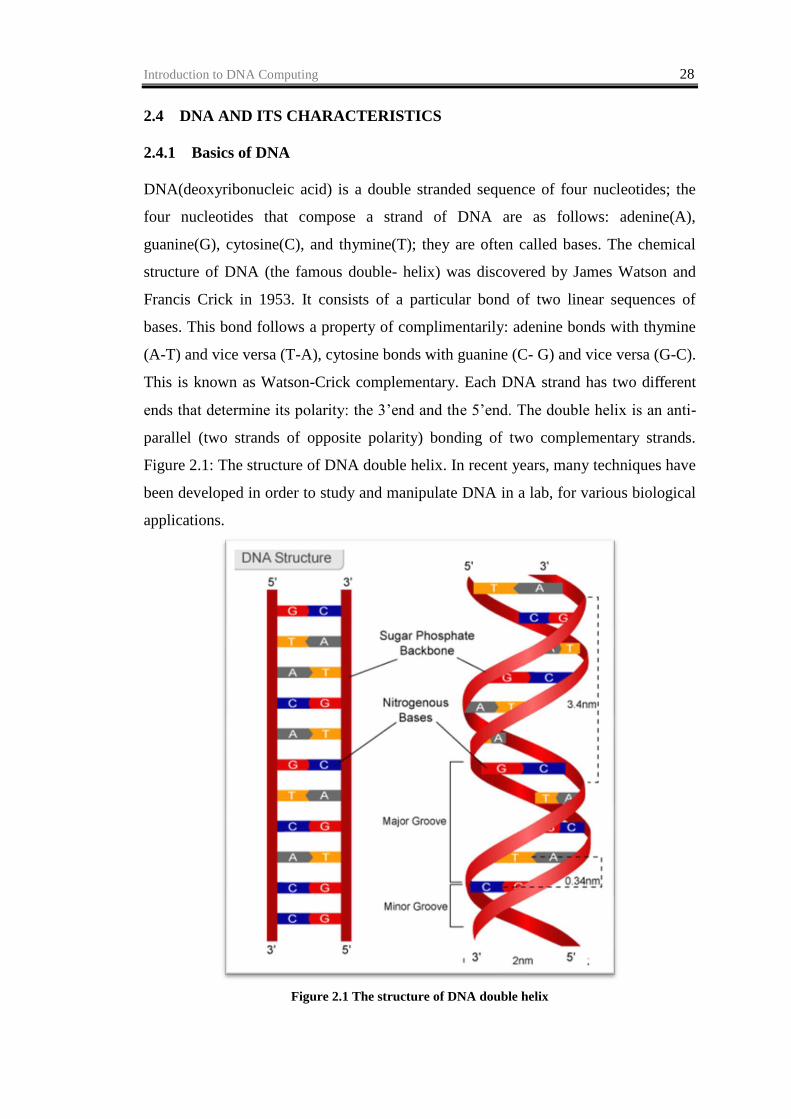
DNA(deoxyribonucleic acid) is a double stranded sequence of four nucleotides; the
four nucleotides that compose a strand of DNA are as follows: adenine(A),
guanine(G), cytosine(C), and thymine(T); they are often called bases. The chemical
structure of DNA (the famous double- helix) was discovered by James Watson and
Francis Crick in 1953. It consists of a particular bond of two linear sequences of
bases. This bond follows a property of complimentarily: adenine bonds with thymine
(A-T) and vice versa (T-A), cytosine bonds with guanine (C- G) and vice versa (G-C).
This is known as Watson-Crick complementary. Each DNA strand has two different
ends that determine its polarity: the 3‘end and the 5‘end. The double helix is an anti-
parallel (two strands of opposite polarity) bonding of two complementary strands.
Figure 2.1: The structure of DNA double helix. In recent years, many techniques have
been developed in order to study and manipulate DNA in a lab, for various biological
applications.
Figure 2.1 The structure of DNA double helix
Introduction to DNA Computing 29
The advances in molecular biology are such that these techniques which are once
considered very sophisticated are now made DNA operations to be routine in all the
molecular biology laboratories. DNA computing makes use of these techniques to
solve some of the difficult problems, which cannot be solved on a computer.
Molecular biology suggests a new way of solving an NP-complete problem. The idea
(due to Leonard Adleman) is to use strands of DNA to encode the (instance of the)
problem and to manipulate them using techniques commonly available in any
molecular biology laboratory, to simulate operations that select the solution of the
problem, if it exists. After Adleman‘s paper [106] appeared in Science in November
1994 many authors have been interested in DNA computing. DNA computing must
not be confused with bio computing. For instance, in bio computing algorithms and
data structures have been developed to investigate the properties of the sequences of
nucleotides in DNA or RNA and those of amino acids in the primary structure of a
protein. In DNA computing, instead, molecular biology is suggested to solve
problems for computer scientists.
Several people made attempts to solve different class of problems including some NP-
complete. The approach is twofold, one being solving a problem with the help of
DNA operations and verifying it in a laboratory and the other being solving a problem
by making use of DNA ‘s main characteristics and proposing a corresponding
algorithm which can be verified more like a theory. But a problem, which is solved
using DNA, involves several operations on DNA
2.4.2 Uniqueness of DNA computing
DNA, with its unique data structure and ability to perform many parallel operations,
allows you to look at a computational problem from a different point of view.
Transistor based computers typically handle operations in a sequential manner. Of
course there are multi-processor computers, and modern CPUs incorporate some
parallel processing, but in general, in the basic Von Neumann Architecture computer,
instructions are handled sequentially. A Von Neumann machine, which is what all
modern CPUs are, basically repeat the same ‖Fetch and execute cycle‖ over and over
again; it fetches an instruction and the appropriate data from main memory, and
Introduction to DNA Computing 30
executes the instruction. It does this many, many times in a row really fast. The great
Richard Feynman, in his Lecture on Computation, summed up Von Neumann
computers by saying,‖The inside of a computer is as dumb as hell but it goes like
mad!‖ DNA computers, however, are non von-Neumann, stochastic machines that
approach computation in a different way from ordinary computers for the purpose of
solving a different class of problems.
Typically, increasing the performance of silicon computing means faster clock cycles
(and larger data paths), where the emphasis is on the speed of CPU and not on the size
of the memory. For example, will doubling the clock speed or doubling your RAM
give you better performance? For DNA computing, the power comes from the
memory capacity and parallel processing. If forced to behave sequentially, DNA loses
its appeal. For example, let‘s look at the read and write rate of DNA. In bacteria,
DNA can be replicated at a rate about 500 base pairs a second. Biologically this is
quite fast (10 times faster than human cells) and considering the low error rates, an
impressive achievement. But this is only 1000bits/sec, which is a snail‘s pace when
compared to the data throughput of an average hard drive. But look what hap- pens if
you allow many copies of the replication enzymes to work on DNA in parallel. First
of all, the replication enzymes can start on the second replicated strand of DNA even
before they‘re finished copying the first one. So, already the data rate jumps to 2000
bits/sec. But look what happens after each replication is finished-the number of DNA
strands increases exponentially (2n after n iterations).With each additional strand, the
additional, the data rate increase by 1000 bits/sec. So after 10 iterations, the DNA is
being replicated at the rate of about 1 Mbit/sec, after 30 iterations it increases to 1000
Gbits/sec. This is beyond the sustained data rates of the faster hard drives.
2.4.3 Motivation for DNA computing
There are three reasons for using DNA computing to solve computational problems
(1). The information density of DNA is much greater than that of silicon: 1 bit can
be stored in approximately one cubic nanometer. Other storage media, such as
videotapes, can store 1 bit in 1,000,000,000,000 cubic nanometer.
Introduction to DNA Computing 31
(2). Operations on DNA are massively parallel: a test tube can contain trillions of
strands. Each operation on a test tube of DNA is carried out on all strands in the
tube in parallel.
(3). DNA computing is an interdisciplinary field where : biologists, computer
scientists, physics, mathematicians, chemists, etc. find a lot of interesting
problems which can be applied to both theoretical and practical areas of DNA
computing.
2.5 NATURE OF DNA COMPUTING
2.5.1 General working aspects
Bio-molecular computers work at the molecular level. Because bio- logical and
mathematical operations have some similarities, DNA, the genetic material that
encodes for living organisms, is stable and predictable in its reactions and can be used
to encode information for mathematical systems. Our computers, with more and more
packed onto their silicon chips are approaching the limits of miniaturization.
Molecular computing may be a way around this limitation.
DNA is the major information storage molecule in living cells, and billions of years of
evolution have tested and refined both this wonderful informational molecule and
highly specific enzymes that can either duplicate the information in DNA molecules
or transmit this information to other DNA molecules.
Instead of using electrical impulses to represent bits of information, the DNA
computer uses the chemical properties of these molecules by examining the patterns
of combination or growth of the molecules or strings. DNA can do this through the
manufacture of enzymes, which are biological catalysts that could be called the
‘software‘, used to execute the desired calculation. DNA computers use
deoxyribonucleic acids A (adenine), C (cytosine), G (guanine) and T (thymine) as the
memory units and recombinant DNA techniques already in existence carry out the
fundamental operations. In a DNA computer, computation takes place in test tubes.
The input and output are both strands of DNA, whose genetic sequences encode
certain information. A program on a DNA computer is executed as a series of
biochemical operations, which have the effect of synthesizing, extracting, modifying
and cloning the DNA strands. Their potential power underscores how nature could be
capable of crunching number better and faster than the most advanced silicon chips.
Introduction to DNA Computing 32
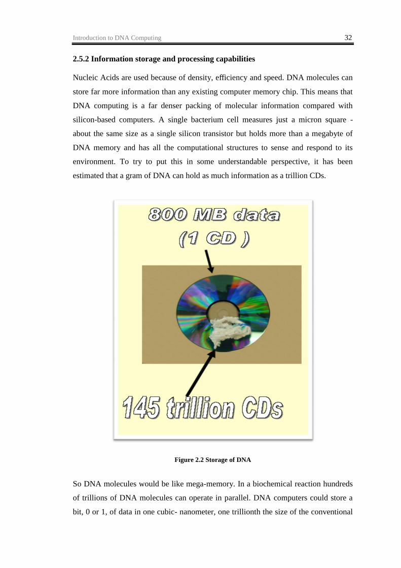
2.5.2 Information storage and processing capabilities
Nucleic Acids are used because of density, efficiency and speed. DNA molecules can
store far more information than any existing computer memory chip. This means that
DNA computing is a far denser packing of molecular information compared with
silicon-based computers. A single bacterium cell measures just a micron square -
about the same size as a single silicon transistor but holds more than a megabyte of
DNA memory and has all the computational structures to sense and respond to its
environment. To try to put this in some understandable perspective, it has been
estimated that a gram of DNA can hold as much information as a trillion CDs.
Figure 2.2 Storage of DNA
So DNA molecules would be like mega-memory. In a biochemical reaction hundreds
of trillions of DNA molecules can operate in parallel. DNA computers could store a
bit, 0 or 1, of data in one cubic- nanometer, one trillionth the size of the conventional
Introduction to DNA Computing 33
computer‘s electronic storage. Thus a DNA computer could store massive quantities
of information in the space a standard computer would use to store much less. A
pound of DNA could contain more computer memory than all the electronic
computers ever made. It would be about twice as fast as the fastest supercomputer,
performing more than 2,000 instructions per second. DNA computers also require
miniscule amounts of energy to perform. ‖We are interested in scale up. We believe
that .we can see scaling up within a few years by a factor of a trillion or more.‖
Because the biochemical operations involved are subject to errors and are often slow,
rigorous tests of the accuracy and further technological development are needed.
2.5.3 Efficiency
In both the solid-surface glass-plate approach and the test tube approach, each DNA
strand represents one possible answer to the problem that the computer is trying to
solve. The strands have been synthesized by combining the building blocks of DNA,
called nucleotides, with one another, using techniques developed for biotechnology.
The set of DNA strands is manufactured so that all conceivable answers are included.
Because a set of strands is tailored to a specific problem, a new set would have to be
made for each new problem.
Most electronic computers operate linearly and they manipulate one block of data
after another, biochemical reactions are highly in parallel: a single step of biochemical
operations can be set up so that it affects trillions of DNA strands. While a DNA
computer takes much longer than a normal computer to perform each individual
calculation, it performs an enormous number of operations at a time and requires less
energy and space than normal computers. 1000 litres of water could contain DNA
with more memory than all the computers ever made, and a pound of DNA would
have more computing power than all the computers ever made.
Obviously if you want to perform one calculation at a time, DNA computers are not a
viable option. When Adleman derived an optimal solution to a seven-city travelling-
salesman problem, it took approximately one week. Unfortunately, you can solve the
same problem on a piece of paper in about an hour or by a digital computer in a few
Introduction to DNA Computing 34
seconds. But when the number of cities is increased to just 70, the problem becomes
intractable for even a 1000-Mips supercomputer.
The only fundamental difference between conventional computers and DNA
computers is the capacity of memory units: electronic computers have two positions
(on or off), whereas DNA has four (C, G, A or T). The study of bacteria has shown
that restriction enzymes can be employed to cut DNA at a specific word (W). Many
restriction enzymes cut the two strands of double-stranded DNA at different positions
leaving overhangs of single-stranded DNA. Two pieces of DNA may be re- joined if
their terminal overhangs are complementary. Complements are referred to as ‘sticky
ends‘. Using these operations, fragments of DNA may be inserted or deleted from the
DNA.
As stated earlier DNA represents information as a pattern of molecules on a strand.
Each strand represents one possible answer. In each experiment, the DNA is tailored
so that all conceivable answers to a particular problem are included. Researchers then
subject all the molecules to precise chemical reactions that imitate the computational
abilities of a traditional computer. Because molecules that make up DNA bind
together in predictable ways, it gives a powerful ‖search‖ function. If the experiment
works, the DNA computer weeds out all the wrong answers, leaving one molecule or
more with the right answer. All these molecules can work together at once, so you
could theoretically have 10 trillion calculations going on at the same time in very little
space.
DNA computing is a field that holds the promise of ultra-dense systems that pack
megabytes of information into devices the size of a silicon transistor. Each molecule
of DNA is roughly equivalent to a little computer chip. Conventional computers
represent information in terms of 0‘s and 1‘s, physically expressed in terms of the
flow of electrons through logical circuits, whereas DNA computers represent
information in terms of the chemical units of DNA. Computing with an ordinary
computer is done with a program that instructs electrons to travel on particular paths;
with a DNA computer, computation requires synthesizing particular sequences of
DNA and letting them react in a test tube or on a glass plate. In a scheme devised by
Richard Lipton, the logical command ‖and‖ is performed by separating DNA strands
Introduction to DNA Computing 35
according to their sequences, and the command ‖or‖ is done by pouring together DNA
solutions containing specific sequences merging.
By forcing DNA molecules to generate different chemical states, which can then be
examined to determine an answer to a problem by combination of molecules into
strands or the separation of strands, the answer is obtained.
Most of the possible answers are incorrect, but one or a few may be correct, and the
computer‘s task is to check each of them and remove the incorrect ones using
restrictive enzymes. The DNA computer does that by subjecting all of the strands
simultaneously to a series of chemical reactions that mimic the mathematical
computations an electronic computer would perform on each possible answer. When the
chemical reactions are complete, researchers analyze the strands to find the answer .For
instance, by locating the longest or the shortest strand and decoding it to determine what
answer it represents.
Computers based on molecules like DNA will not have a Von Neumann architecture,
but instead function best in parallel processing applications. They are considered
promising for problems that can have multiple computations going on at the same
time. Say for instance, all branches of a search tree could be searched at once in a
molecular system while von Neumann systems must explore each possible path in
some sequence.
Information is stored in DNA as CG or AT base pairs with maximum information
density of 2bits per DNA base location. Information on a solid surface is stored in a
NON-ADDRESSED array of DNA words of a fixed length (16mers). DNA Words are
linked together to form large combinatorial sets of molecules. DNA computers are
massively parallel, while electronic computers would require additional hardware;
DNA computers just need more DNA. This could make the DNA computer more
effcient, as well as more easily programmable.
2.5.4 Success of DNA computing
The first applications were ―brute force‖ solutions in which random DNA molecules
were generated, and then the correct sequence was identified. The first problems
solved by DNA computations involved finding the optimal path by which a travelling
Introduction to DNA Computing 36
salesman could visit a fixed number of cities once each. Recent works have shown
how DNA can be employed to carry out a fundamental computer operation, addition
of two numbers expressed in binary (Bancroft) and several other problems like, Max-
Clique Problem, Graph-Colouring Problem, Satisfiability Problem, Bounded Post
Corresponding problem etc
2.5.5 How it works
In November of 1994, Leonard Adleman published a dramatic reminder that
computation is independent of any particular substrate. By using strands of DNA
annealing to each other, he was able to compute a solution to an instance of the
Hamiltonian path problem (HPP) . While working in formal language theory and
artificial selection of RNA had presaged the concept of using DNA to do
computation, these precursors had largely gone unnoticed in mainstream computer
science. Adleman‘s work sparked intense excitement and marked the birth of a new
field, DNA computation
There is no better way to understand how something works than by going through an
example step by step. So let‘s solve our own directed Hamiltonian Path problem,
using the DNA methods demonstrated by Adleman. The concepts are the same but the
example has been simplified to make it easier to follow and present.
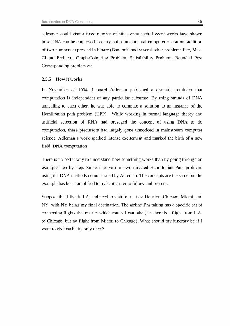
Suppose that I live in LA, and need to visit four cities: Houston, Chicago, Miami, and
NY, with NY being my final destination. The airline I‘m taking has a specific set of
connecting flights that restrict which routes I can take (i.e. there is a flight from L.A.
to Chicago, but no flight from Miami to Chicago). What should my itinerary be if I
want to visit each city only once?
Introduction to DNA Computing 37
Figure 2.3 Directed Hamiltonian Path
It should take you only a moment to see that there is only one route. Starting from
L.A. you need to fly to Chicago, Dallas, Miami and then to N.Y. Any other choice of
cities will force you to miss a destination, visit a city twice, or not make it to N.Y. For
this example you obviously don‘t need the help of a computer to find a solution. For
six, seven, or even eight cities, the problem is still manageable. However, as the
number of cities increases, the problem quickly gets out of hand. Assuming a random
distribution of connecting routes, the number of itineraries you need to check
increases exponentially. Pretty soon you will run out of pen and paper listing all the
possible routes, and it becomes a problem for a computer or perhaps DNA. The
method Adleman used to solve this problem is basically the shotgun approach
mentioned previously. He first generated all the possible itineraries and then selected
the correct itinerary. This is the advantage of DNA. It‘s small and there are
combinatorial techniques that can quickly generate many different data strings. Since
the enzymes work on many DNA molecules at once, the selection process is
massively parallel.
Specifically, the method based on Adleman‘s experiment would be as follows:
1. Generate all possible routes.
2. Select itineraries that start with the proper city and end with the final city.
3. Select itineraries with the correct number of cities.
4. Select itineraries that contain each city only once.
All of the above steps can be accomplished with standard molecular biology
techniques.
Introduction to DNA Computing 38
Part I: Generate all possible routes
Strategy: Encode city names in short DNA sequences. Encode itineraries by
connecting the city sequences for which routes exist.
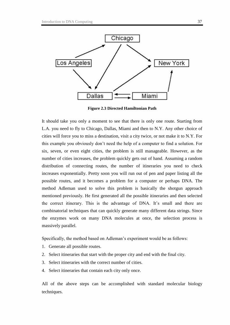
DNA can simply be treated as a string of data. For example, each city can be
represented by a "word" of six bases:
Los Angeles GCTACG
Chicago CTAGTA
Dallas TCGTAC
Miami CTACGG
New York ATGCCG
Table 2.1 DNA Encoded itinerary
The entire itinerary can be encoded by simply stringing together these DNA
sequences that represent specific cities. For example, the route from L.A → Chicago
→Dallas → Miami → New York would simply be as follows: -
GCTACGCTAGTATCGTACCTACGGATGCCG, or equivalently it could be
represented in double stranded form with its complement sequence.
So how do we generate this? Synthesizing short single stranded DNA is now a routine
process, so encoding the city names is straightforward. The molecules can be made by
a machine called a DNA synthesizer or even custom ordered from a third party.
Itineraries can then be produced from the city encodings by linking them together in
proper order. To accomplish this we can take advantage of the fact that DNA
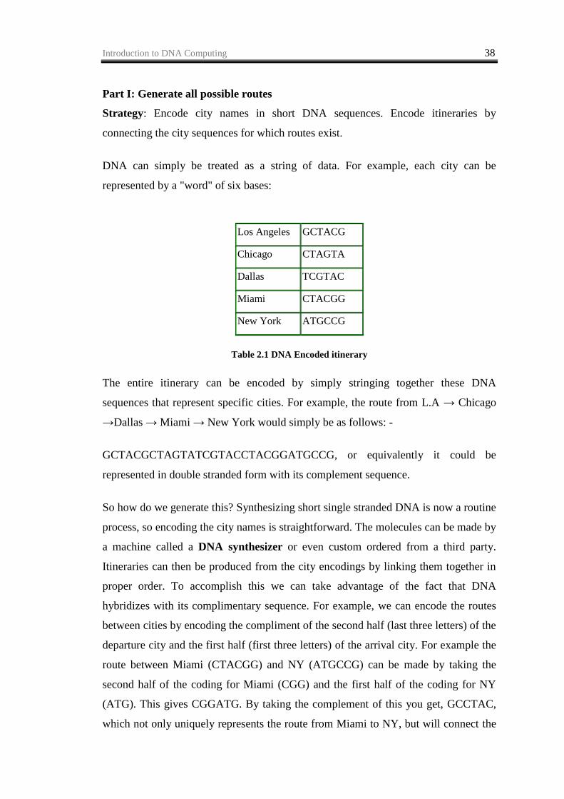
hybridizes with its complimentary sequence. For example, we can encode the routes
between cities by encoding the compliment of the second half (last three letters) of the
departure city and the first half (first three letters) of the arrival city. For example the
route between Miami (CTACGG) and NY (ATGCCG) can be made by taking the
second half of the coding for Miami (CGG) and the first half of the coding for NY
(ATG). This gives CGGATG. By taking the complement of this you get, GCCTAC,
which not only uniquely represents the route from Miami to NY, but will connect the
Introduction to DNA Computing 39
DNA representing Miami and NY by hybridizing itself to the second half of the code
representing Miami (...CGG) and the first half of the code representing NY (ATG...).
For example:
Figure 2.4 DNA Route Encoding
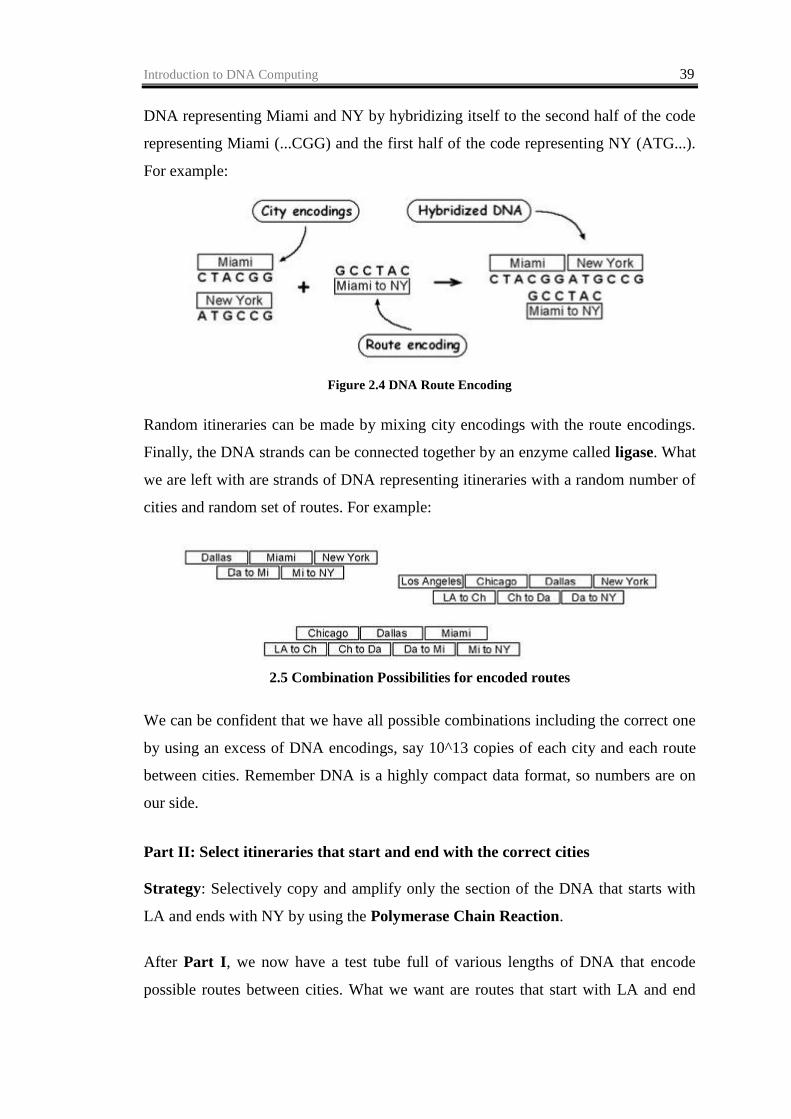
Random itineraries can be made by mixing city encodings with the route encodings.
Finally, the DNA strands can be connected together by an enzyme called ligase. What
we are left with are strands of DNA representing itineraries with a random number of
cities and random set of routes. For example:
2.5 Combination Possibilities for encoded routes
We can be confident that we have all possible combinations including the correct one
by using an excess of DNA encodings, say 10^13 copies of each city and each route
between cities. Remember DNA is a highly compact data format, so numbers are on
our side.
Part II: Select itineraries that start and end with the correct cities
Strategy: Selectively copy and amplify only the section of the DNA that starts with
LA and ends with NY by using the Polymerase Chain Reaction.
After Part I, we now have a test tube full of various lengths of DNA that encode
possible routes between cities. What we want are routes that start with LA and end
Introduction to DNA Computing 40
with NY. To accomplish this we can use a technique called Polymerase Chain
Reaction (PCR), which allows you to produce many copies of a specific sequence of
DNA. PCR is an iterative process that cycles through a series of copying events using
an enzyme called polymerase. Polymerase will copy a section of single stranded
DNA starting at the position of a primer, a short piece of DNA complimentary to one
end of a section of the DNA that you're interested in. By selecting primers that flank
the section of DNA you want to amplify, the polymerase preferentially amplifies the
DNA between these primers, doubling the amount of DNA containing this sequence.
After many iterations of PCR, the DNA you're working on is amplified exponentially.
So to selectively amplify the itineraries that start and stop with our cities of interest,
we use primers that are complimentary to LA and NY. What we end up with after
PCR is a test tube full of double stranded DNA of various lengths, encoding
itineraries that start with LA and end with NY.
Part III: Select itineraries that contain the correct number of cities.
Strategy: Sort the DNA by length and select the DNA whose length corresponds to 5
cities.
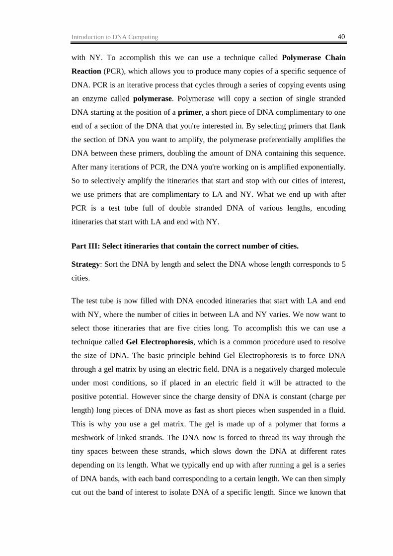
The test tube is now filled with DNA encoded itineraries that start with LA and end
with NY, where the number of cities in between LA and NY varies. We now want to
select those itineraries that are five cities long. To accomplish this we can use a
technique called Gel Electrophoresis, which is a common procedure used to resolve
the size of DNA. The basic principle behind Gel Electrophoresis is to force DNA
through a gel matrix by using an electric field. DNA is a negatively charged molecule
under most conditions, so if placed in an electric field it will be attracted to the
positive potential. However since the charge density of DNA is constant (charge per
length) long pieces of DNA move as fast as short pieces when suspended in a fluid.
This is why you use a gel matrix. The gel is made up of a polymer that forms a
meshwork of linked strands. The DNA now is forced to thread its way through the
tiny spaces between these strands, which slows down the DNA at different rates
depending on its length. What we typically end up with after running a gel is a series
of DNA bands, with each band corresponding to a certain length. We can then simply
cut out the band of interest to isolate DNA of a specific length. Since we known that
Introduction to DNA Computing 41
each city is encoded with 6 base pairs of DNA, knowing the length of the itinerary
gives us the number of cities. In this case we would isolate the DNA that was 30 base
pairs long (5 cities times 6 base pairs).
Figure 2.6 Gel Electrophoresis
Part IV: Select itineraries that have a complete set of cities
Strategy: Successively filter the DNA molecules by city, one city at a time. Since the
DNA we start with contains five cities, we will be left with strands that encode each
city once.
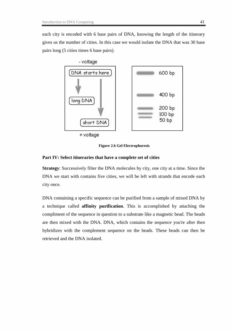
DNA containing a specific sequence can be purified from a sample of mixed DNA by
a technique called affinity purification. This is accomplished by attaching the
compliment of the sequence in question to a substrate like a magnetic bead. The beads
are then mixed with the DNA. DNA, which contains the sequence you're after then
hybridizes with the complement sequence on the beads. These beads can then be
retrieved and the DNA isolated.
Introduction to DNA Computing 42
Figure 2.7 Affinity Purification
So we now affinity purifies five times, using a different city complement for each run.
For example, for the first run we use L.A.'-beads (where the ' indicates compliment
strand) to fish out DNA sequences which contain the encoding for L.A. (which should
be the DNA because of step 3), the next run we use Dallas'-beads, and then Chicago'-
beads, Miami'-beads, and finally NY'-beads. The order isn‘t important. If an itinerary
is missing a city, then it will not be "fished out" during one of the runs and will be
removed from the candidate pool. What we are left with are itineraries that start in
LA, visit each city once, and end in NY. This is exactly what we are looking for. If
the answer exists we would retrieve it at this step.
Reading out the answer
One possible way to find the result would be to simply sequence the DNA strands.
However, since we already have the sequence of the city encodings we can use an
alternate method called graduated PCR. Here we do a series of PCR amplifications
using the primer corresponding to L.A., with a different primer for each city in
succession. By measuring the various lengths of DNA for each PCR product we can
piece together the final sequence of cities in our itinerary. For example, we know that
the DNA itinerary starts with LA and is 30 base pairs long, so if the PCR product for
the LA and Dallas primers was 24 base pairs long, you know Dallas is the fourth city
in the itinerary (24 divided by 6). Finally, if we were careful in our DNA
manipulations the only DNA left in our test tube should be DNA itinerary encoding
LA, Chicago, Miami, Dallas, and NY. So if the succession of primers used is LA &
Introduction to DNA Computing 43
Chicago, LA & Miami, LA & Dallas, and LA & NY, then we would get PCR
products with lengths 12, 18, 24, and 30 base pairs.
Caveats
Adleman's experiment solved a seven city problem, but there are two major
shortcomings preventing a large scaling up of his computation. The complexity of the
traveling salesman problem simply doesn‘t disappear when applying a different
method of solution - it still increases exponentially. For Adleman‘s method, what
scales exponentially is not the computing time, but rather the amount of DNA.
Unfortunately this places some hard restrictions on the number of cities that can be
solved; after the Adleman article was published, more than a few people have pointed
out that using his method to solve a 200 city HP problem would take an amount of
DNA that weighed more than the earth. Another factor that places limits on his
method is the error rate for each operation. Since these operations are not
deterministic but stochastically driven (we are doing chemistry here), each step
contains statistical errors, limiting the number of iterations you can do successively
before the probability of producing an error becomes greater than producing the
correct result. For example an error rate of 1% is fine for 10 iterations, giving less
than 10% error, but after 100 iterations this error grows to 63%.
Let‘s now look a little bit more deeply into the biochemical operation. In the cell,
DNA is modified biochemically by a variety of enzymes, which are tiny protein
machines that read and process DNA according to nature's design. There is a wide
variety and number of these "operational" proteins, which manipulate DNA on the
molecular level. For example, there are enzymes that cut DNA and enzymes that paste
it back together. Other enzymes function as copiers, and others as repair units.
Molecular biology, Biochemistry, and Biotechnology have developed techniques that
allow us to perform many of these cellular functions in the test tube. It's this cellular
machinery, along with some synthetic chemistry, that makes up the palette of
operations available for computation. Just like a CPU has a basic suite of operations
like addition, bit-shifting, logical operators (AND, OR, NOT NOR), etc. that allow it
to perform even the most complex calculations, DNA has cutting, copying, pasting,
repairing, and many others. And note that in the test tube; enzymes do not function
Introduction to DNA Computing 44
sequentially, working on one DNA molecules at a time. Rather, many copies of the
enzyme can work on many DNA molecules simultaneously. So this is the power of
DNA computing that it can work in a massively parallel fashion.
2.6 APPLICATIONS OF DNA COMPUTING
As far as applications are concerned, this can be quite useful in figuring out how to
route telephone calls, plane trips, and basically any problem that can be turned into a
Hamiltonian problem. It is also been claimed that DNA can be used to solve
optimization problems involving business management. This would involve
optimizing the routing of raw materials. It is even said that DNA can be used in
devising the wiring schematics for circuits.
1. Applications making use of ‖classic‖ DNA computing schemes where the use of
massive parallelism holds an advantage over traditional computing schemes,
including potential polynomial time solutions to hard computational problems;
2. Applications making use of the ‖natural‖ capabilities of DNA, including those that
make use of informational storage abilities and those that interact with existing
and emerging biotechnology;
3. Contributions to fundamental research within both computer science and the
physical sciences, especially concerning exploring the limitations of computability
and to understanding and manipulating bimolecular chemistry.
4. Classical DNA computing techniques have already been theoretically applied to a
real life problem: breaking the Data Encryption Standard (DES). Although this
problem has already been solved using conventional techniques in a much shorter
time than pro- posed by the DNA methods, the DNA models are much more
flexible, potent, and cost effective. The brief description about DES as follows.
DES is a method of encrypting 64-bit messages with a 56-bit key, used extensively in
the United States. Electronic keys are normally a string of data used to code and/or
decode sensitive messages. By finding the appropriate key to a set of encrypted
messages, one can either read encoded messages or pose as the sender of such
messages. Using a special purpose electronic computer and differential cryptanalysis,
it has been shown that the key to DES can be found in several days. However, to do
so would require 243 examples of corresponding encrypted and unencrypted
Introduction to DNA Computing 45
messages (known as plain-text/cipher-text pairs) and would slow down by a factor of
256 if the strength of the encrypting key was increased to 64-bits. In it is proposed
that DES could be broken using a DNA based computer and a search algorithm
similar to Adleman‘s original technique. This procedure would be expected to take 4
months, but would only need a single plain-text/cipher-text pair or an example of
cipher text with several plain text candidates to be successful. The feasibility of
applying DNA computation to this problem was also addressed in using a more
refined algorithm (the sticker model approach) which enabled the researchers to
suggest that they could solve the problem using less than a gram of DNA, an amount
that could presumably be handled by a desk top sized machine. Both models would
likely be more cost and energy effective than the expensive electronic processors
required by conventional means, but is entirely theoretical. The first model ignores
error rates incurred though laboratory techniques and the inherent properties of the
DNA are being used. The second model requires an error rate approaching 0.0001,
with higher rates substantially affecting the volume of DNA required. Despite these
assumptions, these models show that existing methods of DNA computation could be
used to solve a real life problem in a way that is both practical and superior to
methods used by conventional computers. In [11] it is also demonstrated that such
benefits can be obtained despite error rates that would be unacceptable in an
electronic computer and that may be unavoidable in a molecular one.
2.7 COMPARISON OF DNA AND CONVENTIONAL ELECTRONIC
COMPUTERS
As we have discussed the concepts and characteristics of DNA Computer, we can
now compare the DNA Computers with Conventional Electronic computers.
2.7.1 Similarities
Transformation of Data
Both DNA computers and electronic computers use Boolean logic (AND, OR,
NAND, NOR) to transform data. The logical command "AND" is performed by
separating DNA strands according to their sequences, and the command "OR" is done
by pouring together DNA solutions containing specific sequences. For example, the
logical statement "X or Y" is true if X is true or if Y is true. To simulate that, the
Introduction to DNA Computing 46
scientists would pour the DNA strands corresponding to "X" together with those
corresponding to [85][102]
Manipulation of Data
Electronic computers and DNA computers both store information in strings, which are
manipulated to do processes. Vast quantities of information can be stored in a test
tube. The information could be encoded into DNA sequences and the DNA could be
stored. To retrieve data, it would only be necessary to search for a small part of it - a
key word, for example by adding a DNA strand designed so that its sequence sticks to
the key word wherever it appears on the DNA [102].
Computation Ability
All computers manipulate data by addition and subtraction. A DNA computer should
be able to solve a satisfiability problem with 70 variables and 1,000 AND-OR
connections. To solve it, assign various DNA sequences to represent 0‘s and 1‘s at the
various positions of a 70 digit binary number. Vast numbers of these sequences would
be mixed together, generating longer molecules corresponding to every possible 70-
digit sequence [85][102].
2.7.2 Differences
Size
Conventional computers are about 1 square foot for the desktop and another square
foot for the monitor. One new proposal is for a memory bank containing more than a
pound of DNA molecules suspended in about 1,000 quarts of fluid, in a bank about a
yard square. Such a bank would be more capacious than all the memories of all the
computers ever made. The first ever-electronic computer took up a large room
whereas the first DNA computer Adleman) was 100 microliters. Adleman dubbed his
DNA computer the TT-100, for test tube filled with 100 microliters, or about one-
fiftieth of a teaspoon of fluid, which is all it took for the reactions to occur.
Representation of Data
DNA computers use Base 4 to represent data, whereas electronic computers use Base
2 in the form of 1‘s and 0‘s. The nitrogen bases of DNA are part of the basic building
Introduction to DNA Computing 47
blocks of life. Using this four letter alphabet, DNA stores information that is
manipulated by living organisms in almost exactly the same way computers work
their way through strings of 1‘s and 0‘s.
Parallelism
Electronic computers typically handle operations in a sequential manner. Of course,
there are multi-processor computers, and modern CPUs incorporate some parallel
processing, but in general, in the basic Von Neumann architecture computer [100],
instructions are handled sequentially. A von Neumann machine, which is what all
modern CPUs are, basically repeats the same "fetch and execute cycle" over and over
again; it fetches an instruction and the appropriate data from main memory, and it
executes the instruction. It does this many, many times in a row, really, really fast.
The great Richard Feynman [88], in his Lectures on Computation, summed up von
Neumann computers by saying, "the inside of a computer is as dumb as hell, but it
goes like mad!" DNA computers, however, are non-von Neuman, stochastic machines
that approach computation in a different way from ordinary computers for the purpose
of solving a different class of problems.
Typically, increasing performance of silicon computing means faster clock cycles
(and larger data paths), where the emphasis is on the speed of the CPU and not on the
size of the memory. For example, will doubling the clock speed or doubling your
RAM give you better performance? For DNA computing, though, the power comes
from the memory capacity and parallel processing. If forced to behave sequentially,
DNA loses its appeal. For example, let's look at the read and write rate of DNA. In
bacteria, DNA can be replicated at a rate of about 500 base pairs a second.
Biologically this is quite fast (10 times faster than human cells) and considering the
low error rates, an impressive achievement. But this is only 1000 bits/sec, which is a
snail's pace when compared to the data throughput of an average hard drive. But look
what happens if you allow many copies of the replication enzymes to work on DNA
in parallel. First of all, the replication enzymes can start on the second replicated
strand of DNA even before they're finished copying the first one. So already the data
rate jumps to 2000 bits/sec. But look what happens after each replication is finished -
the number of DNA strands increases exponentially (2n after n iterations). With each
Introduction to DNA Computing 48
additional strand, the data rate increases by 1000 bits/sec. So after 10 iterations, the
DNA is being replicated at a rate of about 1Mbit/sec; after 30 iterations it increases to
1000 GBits/sec. This is beyond the sustained data rates of the fastest hard drives. Now
let's consider how you would solve a nontrivial example of the travelling salesman
problem (numbers of cities > 10) with silicon vs. DNA. With a von Neumann
computer, one naive method would be to set up a search tree, measure each complete
branch sequentially, and keep the shortest one. Improvements could be made with
better search algorithms, such as pruning the search tree when one of the branches
you are measuring is already longer than the best candidate. A method you certainly
would not use would be to first generate all possible paths and then search the entire
list. Why? Well, consider that the entire list of routes for a 20-city problem could
theoretically take 45 million Gaga Bytes of memory (18! Routes with 7 byte words)
Also for a 100 MIPS computer, it would take two years just to generate all paths
(assuming one instruction cycle to generate each city in every path). However, using
DNA computing, this method becomes feasible! 1015 is just a nanomole of material,
a relatively small number for biochemistry. Also, routes no longer have to be searched
through sequentially. Operations can be done all in parallel.
Material
Obviously, the material used in DNA Computers is different than in Conventional
Electronic Computers. Generally, people take a variety of enzymes such as restriction
nuclease and ligase as the hardware of DNA Computers, encoded double-stranded or
single-stranded DNA molecules as software and data are stored in the sequences of
base pairs. As for conventional electronic computers, electronic devices compose
hardware. Software and data are stored in the organized structure of electronic devices
represented by the electrical signals. The other difference between DNA Computers
and conventional electronic computers in material is the reusability. The materials
used in DNA Computer are not reusable. Whereas an Electronic computer can operate
indefinitely with electricity as its only input, a DNA computer would require periodic
refuelling and cleaning. On the other side, until now, the molecular components used
are still generally specialized. In the current research of DNA Computing, very
different sets of oligonucleotides are used to solve different problems.
Introduction to DNA Computing 49
Methods of Calculation
By synthesizing particular sequences of DNA, DNA computers carry out calculations.
Conventional computers represent information physically expressed in terms of the
flow of electrons through logical circuits. Builders of DNA computers represent
information in terms of the chemical units of DNA. Calculating with an ordinary
computer is done with a program that instructs electrons to travel on particular paths;
with a DNA computer, calculation requires synthesizing particular sequences of DNA
and letting them react in a test tube [102]. As it is, the basic manipulations used for
DNA Computation include Anneal, Melt, Ligate, Polymerase Extension, Cut,
Destroy, Merge, Separate by Length which can also be combined to high level
manipulations such as Amplify, Separate by Subsequence, Append, Mark, Unmark.
And the most famous example of a higher-level manipulation is the polymerase chain
reaction (PCR).
2.8 ADVANTAGES
Parallelism
―The speed of any computer, biological or not, is determined by two factors: (i) how
many parallel processes it has; (ii) how many steps each one can perform per unit
time. The exciting point about biology is that the first of these factors can be very
large: recall that a small amount of water contains about 1022 molecules. Thus,
biological computations could potentially have vastly more parallelism than
conventional ones.‖[92]
Gigantic Memory Capacity
Just as we have discussed, the other implicit characteristic of DNA Computer is its
gigantic memory capacity. Storing information in molecules of DNA allows for an
information density of approximately 1 bit per cubic nanometer. The bases (also
known as nucleotides) of DNA molecules, which represent the minimize unit of
information in DNA Computers, are spaced every 0.34 nanometres along the DNA
molecule (Figure 4), giving DNA a remarkable data density of nearly 18 Megabits per
inch. In two dimensions, if you assume one base per square nanometer, the data
density is over one million Gigabits per square inch. Compare this to the data density
of a typical high performance hard driver, which is about 7 gigabits per square inch --
a factor of over 100,000 smaller[98].
Introduction to DNA Computing 50
Low Power Dissipation
―The potential of DNA-based computation lies in the fact that DNA has a gigantic
memory capacity and also in the fact that the biochemical operations dissipate so little
energy,‖ says University of Rochester computer scientist Mitsunori Ogihara[96].
DNA computers can perform 2 x 10¹⁹ ligation operations per joule. This is amazing,
considering that the second law of thermodynamics dictates a theoretical maximum of
34 x 1019 (irreversible) operations per joule (at 300K). Existing supercomputers
aren‘t very energy-efficient, executing a maximum of 109 operations per joule[83].
Just think about the energy could be very valuable in future. So, this character of
DNA computers can be very important.
Suitable for Combinatorial Problems
From the first day that DNA Computation is developed, Scientists used it to solve
Combinatorial Problems. In 1994, Leonard Adleman used DNA to solve one of
Hamiltonian Path problem -Travelling Salesman problem. After that Lipton used
DNA Computer to break Data Encryption Standard (DES)[86]. And then much of the
work on DNA computing has continued to focus on solving NP-complete and other
hard computational problems. In fact, experiments have proved that DNA Computers
are suitable for solving complex combinatorial problems, even until now, it costs still
several days to solve the problems like Hamiltonian Path problems. But the key point
is that Adleman's original and subsequent works demonstrated the ability of DNA
Computers to obtain tractable solutions to NP-complete and other hard computational
problems, while these are unimaginable using conventional computers.
Clean, Cheap and Available
Besides above characteristics, clean, cheap and available are easily found from
performance of DNA Computer. It is clean because people do not use any harmful
material to produce it and also no pollution generates. It is cheap and available
because you can easily find DNA from nature while it‘s not necessary to exploit
mines and that all the work you should do is to extract or refine the parts that you
need from organism.
2.9 Drawbacks
Occasionally Slow
The speed of each process in DNA Computing is still an open issue until now. In
1994, Adleman‘s experiment took still a long time to perform. The entire experiment
Introduction to DNA Computing 51
took Adleman 7 days of lab work [84]. Adleman asserts that the time required for an
entire computation should grow linearly with the size of the graph. This is true as long
as the creation of each edge does not require a separate process. Practical experiments
proved that when people using DNA to solve more complex problems such like SAT
problems, more and more laborious separation and detection steps are required, which
will only increase as the scale increases. But these problems may be overcome by
using autonomous methods for DNA computation, which execute multiple steps of
computation without outside intervention. Actually, autonomous DNA computations
were first experimentally demonstrated by Hagiya et al.[91]using techniques similar
to the primer extension steps of PCR and by Reif, Seeman et al. [94] using the self-
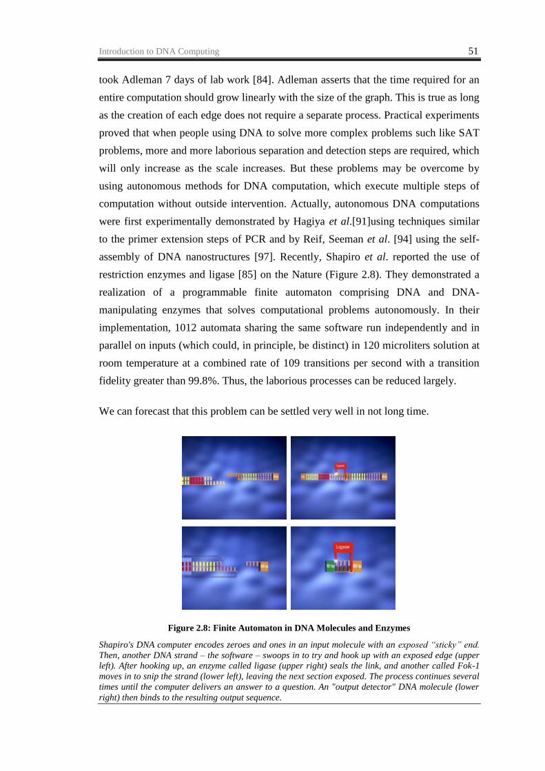
assembly of DNA nanostructures [97]. Recently, Shapiro et al. reported the use of
restriction enzymes and ligase [85] on the Nature (Figure 2.8). They demonstrated a
realization of a programmable finite automaton comprising DNA and DNA-
manipulating enzymes that solves computational problems autonomously. In their
implementation, 1012 automata sharing the same software run independently and in
parallel on inputs (which could, in principle, be distinct) in 120 microliters solution at
room temperature at a combined rate of 109 transitions per second with a transition
fidelity greater than 99.8%. Thus, the laborious processes can be reduced largely.
We can forecast that this problem can be settled very well in not long time.
Figure 2.8: Finite Automaton in DNA Molecules and Enzymes
Shapiro's DNA computer encodes zeroes and ones in an input molecule with an exposed “sticky” end.
Then, another DNA strand – the software – swoops in to try and hook up with an exposed edge (upper
left). After hooking up, an enzyme called ligase (upper right) seals the link, and another called Fok-1
moves in to snip the strand (lower left), leaving the next section exposed. The process continues several
times until the computer delivers an answer to a question. An "output detector" DNA molecule (lower
right) then binds to the resulting output sequence.
Introduction to DNA Computing 52
Hydrolysis
The DNA molecules can fracture. Over the six months you're computing, your DNA
system is gradually turning to water. DNA molecules can break – meaning a DNA
molecule, which was part of your computer, is fracture by time. DNA can deteriorate. As
time goes by, your DNA computer may start to dissolve. DNA can get damaged as it
waits around in solutions and the manipulations of DNA are prone to error. Some
interesting studies have been done on the reusability of genetic material in more
experiments, a result is that it is not an easy task recovering DNA and utilizing it again.
Information not transmittable
The model of the DNA computer is concerned as a highly parallel computer, with
each DNA molecule acting as a separate process. In standard multiprocessor
connection-buses transmit information from one processor to the next. But the
problem of transmitting information from one molecule to another in a DNA
computer has not yet to be solved. Current DNA algorithms compute successfully
without passing any information, but this limits their flexibility.
Reliability Problems
Errors in DNA Computers happen due to many factors. In 1995, Kaplan et al. [89].set
out to replicate Adleman‘s original experiment, and failed. Or to be more accurate,
they state, ―At this time, we have carried out every step of Adleman‘s experiment, but
we have not got an unambiguous final result.‖
Annealing Errors
In Adleman‘s experiment, the first step for DNA computation is to add the strands,
which stand for cities and intercity paths, into a solution of water, ligase, salt, and a
few other ingredients. The strands then combine with their proper DNA complements
to solve the problem in a manner of seconds through the process of annealing (or
"hybridization"). But there are errors that can occur during annealing, though. Its
success varies depending on many factors including temperature, salt content of the
solution, and the proportion of G's and C's in relation to T's and A's in the sequences.
Ideally the DNA will only form perfect matches during annealing. However, one or
Introduction to DNA Computing 53
two base mismatch can also occur and cause interesting results. Well, actually, The
Watson-Crick complement is not universally respected sometimes:
Perfect Match Single base Mismatch Two base Mismatch
3'-ATAACCCCCAATCCT-5' 3'-ATAACCCCCAATCCT-5' 3'-ATAACCCCCAATCCT-5'
5'-TATTGGGGGTTAGGA-3' 5'-TATTGGGGGATAGGA-3' 5'-TATTGGGCGTAAGGA-3'
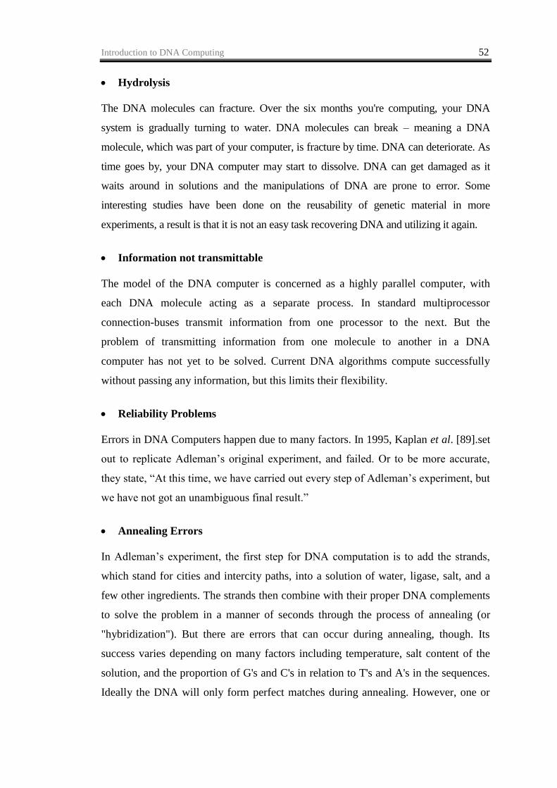
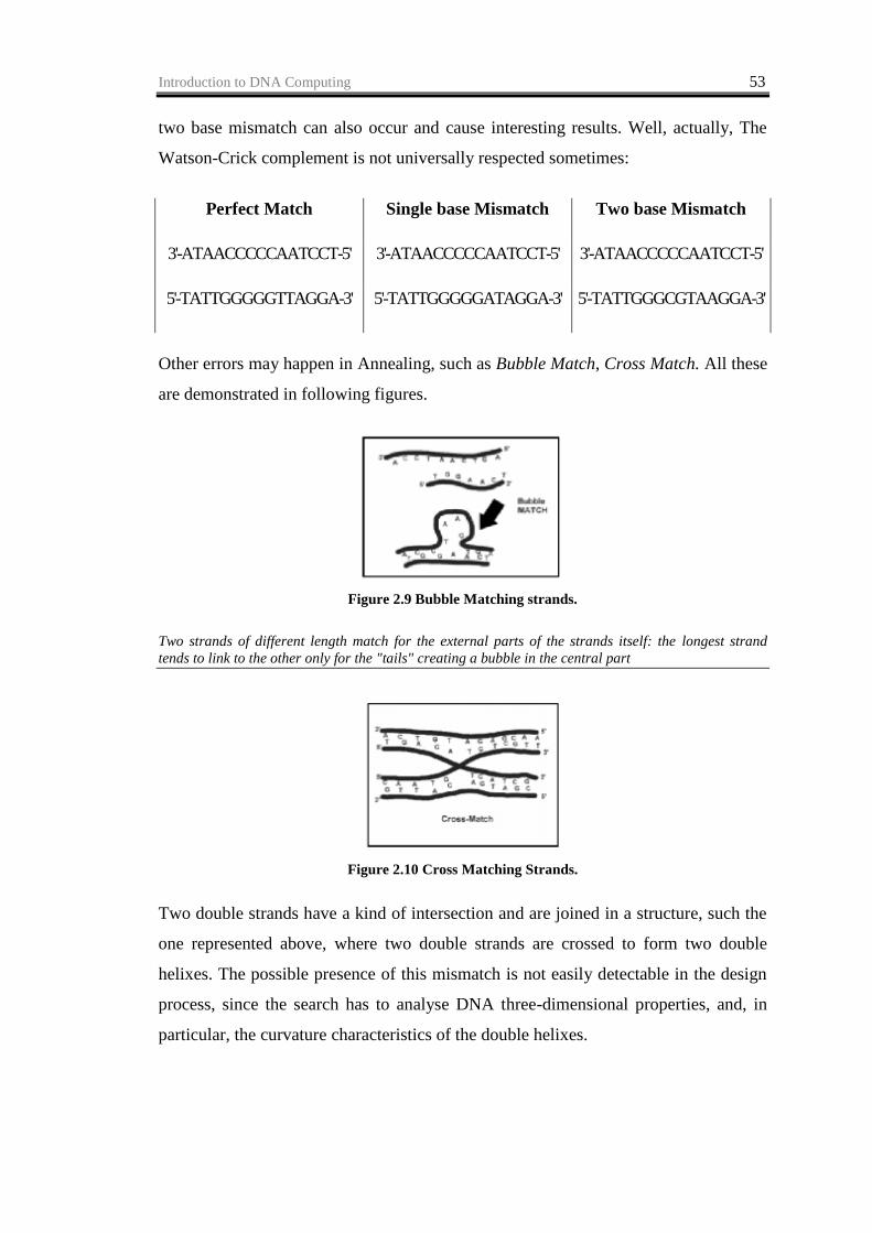
Other errors may happen in Annealing, such as Bubble Match, Cross Match. All these
are demonstrated in following figures.
Figure 2.9 Bubble Matching strands.
Two strands of different length match for the external parts of the strands itself: the longest strand
tends to link to the other only for the "tails" creating a bubble in the central part
Figure 2.10 Cross Matching Strands.
Two double strands have a kind of intersection and are joined in a structure, such the
one represented above, where two double strands are crossed to form two double
helixes. The possible presence of this mismatch is not easily detectable in the design
process, since the search has to analyse DNA three-dimensional properties, and, in
particular, the curvature characteristics of the double helixes.
Introduction to DNA Computing 54
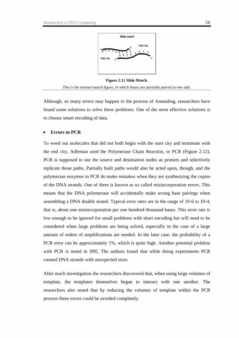
Figure 2.11 Slide Match.
This is the normal match figure, in which bases are partially paired at one side.
Although, so many errors may happen in the process of Annealing, researchers have
found some solutions to solve these problems. One of the most effective solutions is
to choose smart encoding of data.
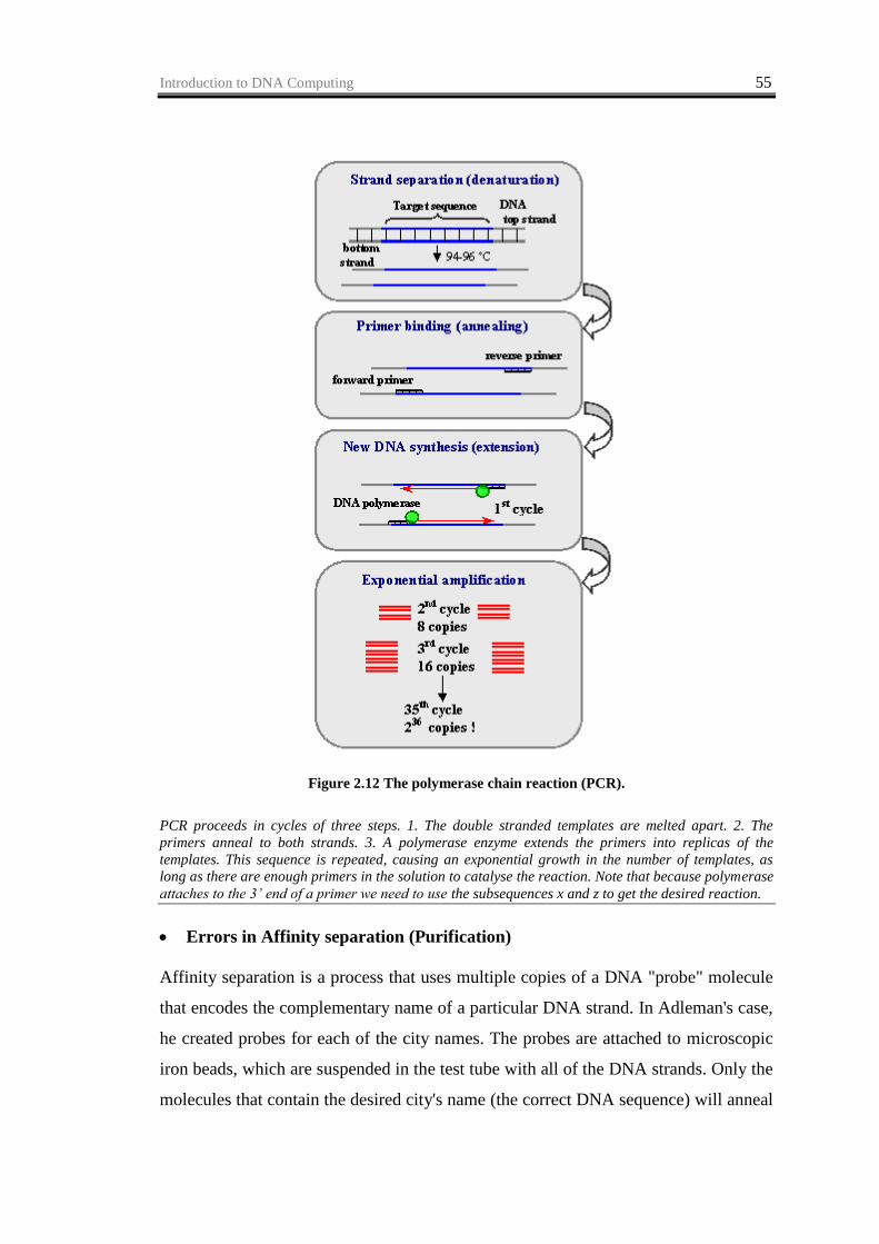
Errors in PCR
To weed out molecules that did not both begin with the start city and terminate with
the end city, Adleman used the Polymerase Chain Reaction, or PCR (Figure 2.12).
PCR is supposed to use the source and destination nodes as primers and selectively
replicate those paths. Partially built paths would also be acted upon, though, and the
polymerase enzymes in PCR do make mistakes when they are synthesizing the copies
of the DNA strands. One of them is known as so called misincorporation errors. This
means that the DNA polymerase will accidentally make wrong base pairings when
assembling a DNA double strand. Typical error rates are in the range of 10-6 to 10-4,
that is, about one misincorporation per one hundred thousand bases. This error rate is
low enough to be ignored for small problems with short encoding but will need to be
considered when large problems are being solved, especially in the case of a large
amount of orders of amplifications are needed. In the later case, the probability of a
PCR error can be approximately 1%, which is quite high. Another potential problem
with PCR is noted in [89]. The authors found that while doing experiments PCR
created DNA strands with unexpected sizes.
After much investigation the researchers discovered that, when using large volumes of
template, the templates themselves began to interact with one another. The
researchers also noted that by reducing the volumes of template within the PCR
process these errors could be avoided completely.
Introduction to DNA Computing 55
Figure 2.12 The polymerase chain reaction (PCR).
PCR proceeds in cycles of three steps. 1. The double stranded templates are melted apart. 2. The
primers anneal to both strands. 3. A polymerase enzyme extends the primers into replicas of the
templates. This sequence is repeated, causing an exponential growth in the number of templates, as
long as there are enough primers in the solution to catalyse the reaction. Note that because polymerase
attaches to the 3’ end of a primer we need to use the subsequences x and z to get the desired reaction.
Errors in Affinity separation (Purification)
Affinity separation is a process that uses multiple copies of a DNA "probe" molecule
that encodes the complementary name of a particular DNA strand. In Adleman's case,
he created probes for each of the city names. The probes are attached to microscopic
iron beads, which are suspended in the test tube with all of the DNA strands. Only the
molecules that contain the desired city's name (the correct DNA sequence) will anneal
Introduction to DNA Computing 56
to the probe. A magnet then attracts the metal beads (and the attached DNA) to the
side while the remaining liquid and DNA is poured out. This process is repeated for
each different city, so that by the end, the strands that are left contain every city. But
in practice, there is always an accepted error rate of 5% in this process. That is to say
that 5% of the time the process will not filter out strings that it should or it will filter
strings that it should not. This error rate does not seem unusually high until you
consider that an algorithm may perform this operation tens or hundreds of times. This
translates to a less than 1% chance of a ―good‖ string surviving the entire process if it
is iterated one hundred times. So this is very pessimistic.
But there is hope however; people have developed techniques for increasing the
survival probability of a given string , that is, decreasing the error rates in Affinity
separation. One of the techniques is to use PCR periodically to increase the number of
strands in the solution. The idea for this technique is to try and make the algorithm
constant volume, which actually on the basis of the fact that through the process of
affinity purification the number of DNA strands in solution is always reduced, or we
say, the affinity purification process is volume decreasing. Another technique is an
alteration of the encoding scheme. The idea of the altered encoding scheme is to
encode all of the information twice. The purpose of doing this is to increase the
probability that affinity purification will successfully filter ―good‖ strings by
increasing the number of possible binding locations.
So will DNA ever be used to solve a traveling salesman problem with a higher
number of cities than can be done with traditional computers? Well, considering that
the record is a whopping 13,509 cities, it certainly will not be done with the procedure
described above. It took this group only three months, using three Digital AlphaServer
4100s (a total of 12 processors) and a cluster of 32 Pentium-II PCs. The solution was
possible not because of brute force computing power, but because they used some
very efficient branching rules. This first demonstration of DNA computing used a
rather unsophisticated algorithm, but as the formalism of DNA computing becomes
refined, new algorithms perhaps will one day allow DNA to overtake conventional
computation and set a new record.
Introduction to DNA Computing 57
And of course we are talking about DNA here, the genetic code of life itself. It
certainly has been the molecule of this century and most likely the next one.
Considering all the attention that DNA has garnered, it isn‘t too hard to imagine that
one day we might have the tools and talent to produce a small integrated desktop
machine that uses DNA, or a DNA-like biopolymer, as a computing substrate along
with set of designer enzymes. Perhaps it won‘t be used to play Quake IV or surf the
web -- things that traditional computers are good at -- but it certainly might be used in
the study of logic, encryption, genetic programming and algorithms, automata,
language systems, and lots of other interesting things that haven't even been invented
yet.