1

Chapter 2 Equilibrium Thermodynamics and Kinetics

Equilibrium thermodynamics predicts the concentrations (or, more precisely, activities) of

various species and phases if a reaction reaches equilibrium. Kinetics tells us how fast, or if, the

reaction will reach equilibrium. Thermodynamics is an elegant way to deal with problems of

chemical equilibria, but it is important to note that kinetics will determine if these equilibrium

conditions are actually attained. In the following sections we will consider these topics in the

context of the typical conditions found in the surface and shallow subsurface environments.

THE LAWS OF THERMODYNAMICS

Thermodynamic principles are applied to systems. A system is that portion of the universe we wish

to study, e.g., a beaker containing a solution, a room, the ocean, planet earth, the universe. The

system can be open (exchanging matter and energy with its surroundings), closed (not exchanging

matter with its surroundings), or isolated (exchanges neither matter nor energy with its

surroundings). As an example, consider a beaker of water standing on a table. The system is open

because it can exchange both heat with the surroundings and gases with the atmosphere. Now seal

the top of the beaker. The result is a closed system because it cannot exchange matter (gases) with

the atmosphere. If we place the beaker in a thermos bottle, it becomes an isolated system because it

can exchange neither heat nor matter with its surroundings.

The properties of a system can be either intensive or extensive. Intensive properties are

independent of the magnitude of the system. Examples are pressure and temperature. Extensive

properties are dependent on the magnitude of the system. Examples are volume and mass.

A system can be described in terms of phases and components. A phase is defined as "a

uniform, homogeneous, physically distinct, and mechanically separable portion of a system”

(Nordstrom and Munoz, 1986, p. 67). Components are the chemical constituents (species) needed

to completely describe the chemical composition of every phase in a system. The choice of

components is determined by the physical-chemical conditions of the system. For example,

consider the three-phase system solid water (ice)–liquid water–water vapor that would exist under

normal surface conditions. The composition of each phase can be completely described by a single

component—H2O. Now consider the same system over a much wider range of temperatures so that

a fourth phase, plasma, is found. In a plasma, the H2O would break down into hydrogen and

2

oxygen atoms. To completely describe the composition of this system we would need two

components—H and O. The solid, liquid, and vapor phases of H2O would be formed by combining

the two components in the proportions 2H + O → H2O.

First Law of Thermodynamics

The first law of thermodynamics deals with the conservation of energy. One statement of the law

is that energy can be neither created nor destroyed, it can only be changed from one form to

another. The concept of enthalpy (heat flow) arises from the first law.

The internal energy of a system is the sum of the kinetic and potential energies of its

constituent atoms. Let us change the internal energy of this system by adding (or subtracting) heat

and by doing mechanical work (on or by the system). We can write the following equation:

∆E = q – w (2–1)

where ∆E is the change in internal energy of the system, q is the heat added or removed from the

system, and w is the work done on or by the system. By convention, heat added to a system is

positive and work done by a system is positive. Thus, the internal energy of a system will increase

if heat is added and will decrease if work is done by the system. For infinitesimal changes,

equation 2–1 can be written

dE = dq – dw (2–2)

If the work done by or on a system causes a change in volume at constant pressure (pressure–

volume work), then the equation for the change in internal energy can be written

∆E = q – P ∆V (2–3)

For an infinitesimal change, equation 2–3 can be written

dE = dq – P dV (2–4)

Enthalpy is equal to the heat flow when processes occur at constant pressure and the only work

done is pressure–volume work. This is the most likely situation in the natural surface environment.

For an infinitesimal change, enthalpy can be written

3

dH = dE + P dV + V dP (2–5)

At constant P, dP = 0 and

dH = dE + P dV (2–6)

If we substitute for dE (equation 2–4), then dH equals dq at constant P.

dH = (dq – P dV) + P dV = dq (2–7)

Note that it is very difficult to determine absolute values for either internal energy (E) or enthalpy

( H) . Hence, these values are determined on a relative basis compared to standard conditions (see

later). Exothermic reactions release heat energy (i.e., enthalpy is negative for the reaction), and

endothermic reactions use heat energy (i.e., enthalpy is positive for the reaction).

The heat of formation (sometimes called the enthalpy of formation or the standard heat of

formation) is the enthalpy change that occurs when a compound is formed from its elements at

particular temperature and pressure (the standard state). It is convenient to use 25°C and 1 bar as

the temperature and pressure for the standard state. Hence, the standard state for a gas is the ideal

gas at 1 bar and 25°C, for a liquid it is the pure liquid at 1 bar and 25°C, and for a solid it is a

specified crystalline state at 1 bar and 25 °C. The heat of formation of the most stable form of an

element is arbitrarily set equal to zero. For example, the heat of formation for La metal and N2 (g)

equals zero. For dissolved ionic species, the heat of formation of H+ is set equal to zero.

Second Law of Thermodynamics

The second law of thermodynamics deals with the concept of entropy. One statement of the law is

that for any spontaneous process, the process always proceeds in the direction of increasing

disorder. Another way of looking at this law is that during any spontaneous process there is a

decrease in the amount of useable energy. As a simple example of the second law consider the

burning of coal. In coal the atoms are ordered; i.e., they occur as complex organic molecules.

During the combustion process these molecules are broken down, with the concomitant release of

energy and the production of CO2 and H2O. The atoms are now in a much more disordered

(dispersed) state. In order to produce more coal we need to recombine these atoms which requires

energy—in fact, more energy than was released by the burning of the coal. Hence, there has been a

4

decrease in the amount of useable energy.

The second law has important practical and philosophical implications. During any process

there is a decline in the amount of useable energy. This is an important concept in ecology in terms

of the efficiency of ecosystems. As a rough rule of thumb, in biological systems about 90% of the

energy is lost in going from one trophic level (nourishment level) to another. For example, for

every 1000 calories of “grass energy” consumed by a cow, only 100 calories are converted to

biomass. If the cow ends up as a steak, only 10% of the energy in the cow’s biomass ends up as

human biomass. Thus, vegetarians are more efficient users of primary biomass (green plants) than

meat eaters. The second law of thermodynamics also predicts that at some point the universe will

cease to function. A way of looking at this is to divide the universe into a high-temperature

reservoir—the stars—and a low-temperature reservoir—the interstellar medium. As energy is lost

from the stars to the interstellar medium, the temperature of the interstellar medium will rise. At

some point, the temperatures of these reservoirs will become equal and energy transfers will cease.

This has sometimes been referred to as the “heat death of the universe.”

A mathematical statement of the second law is

qS

T

(2–8)

where ∆S is the change in entropy and T is temperature in Kelvin (the absolute temperature scale).

Rearranging equation 2–8 to give q = T∆S and substituting into equation 2–1 gives

∆E = T∆S – w (2–9)

Or, in differential form,

dE= T dS – dw (2–10)

If we consider only pressure–volume work, then equation 2–10 becomes

dE = T dS – P dV (2–11)

Substitution of equation 2–11 into equation 2–5 yields

dH = (T dS – P dV) + P dV + V dP = T dS + V dP (2–12)

5

EQUILIBRIUM THERMODYNAMICS

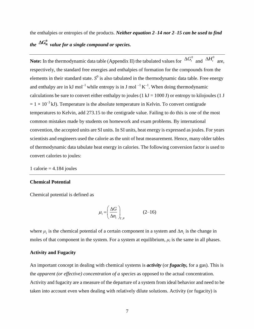
In the real world, systems can exist in several states: unstable, metastable, and stable. To illustrate

these different states, consider a ball sitting at the top of a hill (Figure 2–1). In terms of

gravitational energy, the lowest energy state is achieved when the ball is at the bottom of the hill.

At the top the ball is unstable with respect to gravitational energy. The least disturbance will cause

the ball to start rolling down the hill. Partway down the hill there is a small notch. If the ball does

not have enough energy to roll up over the lip of the notch, it will be stuck at this position. Clearly,

this is not the lowest possible energy state, which occurs at the bottom of the hill, and the ball is

said to be in metastable equilibrium. However, it can remain indefinitely at this position if there

isn’t enough energy available to push it over the lip of the notch. This is an example of a kinetic

impediment to the achievement of equilibrium, and we can regard the energy needed to push the

ball out of the notch to be equivalent to the activation energy. Activation energy will be discussed

in the latter part of this chapter. If sufficient energy is put into the system to push the ball out of the

notch, it will roll to the bottom of the hill. At this position, the gravitational potential energy equals

zero and the ball has achieved its equilibrium position in terms of gravitational energy. In

equilibrium thermodynamics it is this lowest energy state that is determined.

Figure 2–1 Illustration of the states of a system in terms of the gravitational energy of a ball.

6

Free Energy

A system at equilibrium is in a state of minimum energy. In chemical thermodynamics this energy

is measured either as Gibbs free energy (when the reaction occurs at constant T and P) or

Helmholtz free energy (when the reaction occurs at constant T and V). Here we will use Gibbs free

energy, named for J. Willard Gibbs, a Yale University chemist.

For a system at constant T and P, Gibbs free energy can be written

G = H – TS (2–13)

where H is enthalpy (kJ mol–1

), S is entropy (J mol–1

K–1

), and T is temperature in K (Kelvin).

For changes that occur at constant T and P, the expression for Gibbs free energy becomes

ΔG = ΔH – ΤΔS (2–14)

If ΔG is (–), the process occurs spontaneously. If ΔG = 0, the process is at equilibrium. If ΔG is (+),

the reaction does not occur spontaneously. Note that chemical reactions are written from left to

right. For example, consider the reaction

2+ 2

4 anhydrite 4CaSO Ca +SO

If the process occurs spontaneously, CaSO4 will dissolve to form Ca2+

and 2

4SO

ions (i.e., the

reaction is running from left to right). If the process is at equilibrium, the concentration of the

various species remains constant. If the process does not occur spontaneously, the reaction would

actually run from right to left. In the last case, if you rewrote the equation so that the ions were on

the left side and the compound on the right side, the free energy would be negative.

We now write equation 2–14 as follows:

0 0 0

R R RG H T S (2–15)

where 0

RG is the free-energy change,

0

RH is the enthalpy change, and

0

RS is the entropy

change for the reaction at standard conditions. The enthalpy and entropy changes are calculated,

respectively, by subtracting the sum of the enthalpies or entropies of the reactants from the sum of

7

the enthalpies or entropies of the products. Neither equation 2–14 nor 2–15 can be used to find

the

0

RG

value for a single compound or species.

Note: In the thermodynamic data table (Appendix II) the tabulated values for 0

tG and

0

tH are,

respectively, the standard free energies and enthalpies of formation for the compounds from the

elements in their standard state. S0 is also tabulated in the thermodynamic data table. Free energy

and enthalpy are in kJ mol–1

while entropy is in J mol – 1

K–1

. When doing thermodynamic

calculations be sure to convert either enthalpy to joules (1 kJ = 1000 J) or entropy to kilojoules (1 J

= 1 × 10–3

kJ). Temperature is the absolute temperature in Kelvin. To convert centigrade

temperatures to Kelvin, add 273.15 to the centigrade value. Failing to do this is one of the most

common mistakes made by students on homework and exam problems. By international

convention, the accepted units are SI units. In SI units, heat energy is expressed as joules. For years

scientists and engineers used the calorie as the unit of heat measurement. Hence, many older tables

of thermodynamic data tabulate heat energy in calories. The following conversion factor is used to

convert calories to joules:

1 calorie = 4.184 joules

Chemical Potential

Chemical potential is defined as

,

i

i T P

G

n

(2–16)

where μ¡ is the chemical potential of a certain component in a system and ∆n¡ is the change in

moles of that component in the system. For a system at equilibrium, μi is the same in all phases.

Activity and Fugacity

An important concept in dealing with chemical systems is activity (or fugacity, for a gas). This is

the apparent (or effective) concentration of a species as opposed to the actual concentration.

Activity and fugacity are a measure of the departure of a system from ideal behavior and need to be

taken into account even when dealing with relatively dilute solutions. Activity (or fugacity) is

8

related to concentration through the activity coefficient.

ii

i

a

m

(2–17)

where γi is the activity coefficient, ai is the activity, and mi is the actual concentration. Rearranging

equation 2–17 gives

ai = γimi (2–18)

A later section will deal with the calculation of the activity coefficient.

The Equilibrium Constant

We can write the chemical potential for component i as follows:

0 lni i iRT a (2–19)

where 0

i is the chemical potential of component i in its standard state and R is the gas constant

(8.3143 J mol–1

K–1

). For solid solutions, solutions of two miscible liquids, and the solvent in

aqueous solutions, the standard state is the pure substance at the same temperature and pressure.

Let us suppose we have a chemical reaction of the form

aA + bB ⇌ cC + dD (2–20)

The uppercase letters represent the species and the lowercase letters represent the number of each

species (each chemical entity). What follows is an exercise in letter manipulation, a common

activity in the sciences and mathematics. To determine the change in free energy for the system,

we subtract the free energies of the products (right side of the equation) from the free energy of the

reactants (left side of the equation).

∆Greaction =Σ ∆Gproducts – ∆Greactants (2–21)

From the definition of chemical potential (equation 2–16),

∆G = niμi (2–22)

9

and, on substitution, equation 2–21 becomes

∆GR =cμc + dμd – aμa – bμb (2–23)

We substitute equation 2–19 for μi and write equation 2–23 as follows:

c d0 0 0 0 C D

R C D A B a b

A B

a ac d a b ln

a aG RT

(2–24)

The portion of equation 2–24 dealing with the chemical potentials in the standard state is

equivalent to ∆G0, and thus equation 2–24 reduces to

c d0 C D

R R a b

A B

a aln

a aG G RT

(2–25)

At equilibrium, ∆GR = 0 and equation 2–25 becomes

c d0C DRa b

A B

a aln

a aRT G

(2–26)

Dividing both sides of equation 2–26 by R, T, and converting the natural log to an exponent, gives

c d 0

C D Req a b

A B

a aexp

a a

GK

RT

(2–27)

For our last manipulation we will rearrange equation 2–27 to yield

0

Reqln

GK

RT

(2–28)

Note that in equation 2–28 we are calculating the natural log of Keq. A natural log result can be

converted to a base 10 log result by dividing by 2.30259, or by using the proper keystroke

sequence on a calculator. If the reactions of interest are occurring at 25°C and 1 bar and the free

energy is in kJ mol–1

, equation 2–28 can be written in base 10 log form as

0

Reqlog

5.708

GK

(2–29)

10

Equation 2–29 can only be used for reactions occurring at 25 °C and 1 bar. We have now

completed our exercise in letter manipulation and everyone should feel very refreshed. The

following example illustrates the calculation of an equilibrium constant.

A word about thermodynamic data. There are a number of data compilations in the literature.

You may find that for any particular species the different compilations do not give the same value.

Thermodynamic data are determined experimentally and are thus subject to error. In compiling a

set of thermodynamic data, the compilers attempt to make the data internally consistent; i.e.,

calculations using the data set give reasonable and consistent answers. Where values have been

determined by more than one laboratory, a judgment must be made by the compilers as to which

values are more consistent with their data set. In addition, errors can creep into compilations,

which can lead to some rather paradoxical answers. The user must be aware of these potential

pitfalls. When using a water-chemistry computer model, you should take note of the

thermodynamic database used by the model.

EXAMPLE 2–1 Calculate the solubility product for gypsum at 25°C. The solubility product is a

special form of an equilibrium constant (i.e., it enables us to calculate the activity of the ions in

solution at saturation).

The reaction is

2+ 2

4 2 gypsum 4 2CaSO 2H O Ca SO 2H O

The equilibrium equation is written

22 2

4 2

4 2 gypsum

Ca SO H O

CaSO 2H OeqK

Note that the various species are enclosed in brackets. The convention is that enclosing the species

in brackets indicates activity, while enclosing the species in parentheses indicates

concentrations. CaSO4·2H2O is in its standard state (pure solid) and its activity equals 1. For a

dilute solution, the activity of water also equals 1. The activity of water in cases other than dilute

solutions is considered in a later section. For the dissolution of gypsum, the equilibrium equation

11

becomes

2 2

4 spCa SOeqK K

Selecting the appropriate free energies of formation (Appendix II, source 2) yields (remember,

products – reactants)

0 1552.8 744.0 2 237.14 1797.36 26.28kJmolRG

04.60

sp sp

26.28log 4.60, 10

5.708 5.708

RGK K

Henry's Law

This relationship is used in several ways. In solutions, it is used to describe the activity of a dilute

component as a function of concentration. In this case, the relationship is written

ai = hiXi (2–30)

where ai is the activity of species i, hi is the Henry’s law proportionality constant, and Xi is the

concentration of species i.

For gases, Henry’s law relates the fugacity of the gas to its activity in solution. At total

pressures of 1 bar or less and temperatures near surface temperatures, gases tend to obey the ideal

gas law, and hence the fugacity of a gas equals its partial pressure. In this case, we write Henry’s

law as

Ci = KHPi (2–31)

12

Table 2–1 Henry's Law Constants for Gases at 1 Bar Total Pressure in Mol L–1

Bar– 1

*

T( °C ) O2 N2 CO2 H2S SO2

0 2.18 × 10–3

1.05 × 10–3

7.64 × 10–2

2.08 × 10–1 3.56

5 1.91 × 10–3

9.31 × 10–4

6.35 × 10–2

1.77 × 10–1 3.01

10 1.70 × 10–3

8.30 × 10–4

5.33 × 10–2

1.52 × 10–1 2.53

15 1.52 × 10–3

7.52 × 10–4

4.55 × 10–2 1.31 × 10

–1 2.11

20 1.38 × 10–3

6.89 × 10–4 3.92 × 10

–2 1.15 × 10

–1 1.76

25 1.26 × 10–3

6.40 × 10–4

3.39 × 10–2

1.02 × 10–1 1.46

30 1.16 × 10–3

5.99 × 10–4

2.97 × 10–2

9.09 × 10–2 1.21

35 1.09 × 10–3

5.60 × 10–4

2.64 × 10–2

8.17 × 10–2 1.00

40 1.03 × 10–3

5.28 × 10–4

2.36 × 10–2

7.41 × 10–2 0.837

50 9.32 × 10–4

4.85 × 10–4

1.95 × 10–2

6.21 × 10–2

—

*Data are from Pagenkopf (1978).

where Ci is the concentration of the gaseous species in solution, KH is the Henry’s law constant in

mol L–1

bar–1

, and Pi is the partial pressure of gaseous species i. Henry’s law constants vary as a

function of temperature (Table 2–1). We will use Henry’s law in later chapters to calculate the

activity of various gases dissolved in water and the partial pressure of various volatile organic

solvents.

EXAMPLE 2–2 Calculate the solubility of oxygen in water at 20°C.

At sea level—i.e., a total atmospheric pressure of 1 bar (in terms of the standard atmosphere,

precisely 1.0135 bar)—the partial pressure of oxygen is 0.21 bar. At 20°C, the Henry’s law

constant for oxygen is 1.38 × 10–3

mol L–1

bar–1

.

13

O2 (aq) = 2H OK P = (1.38 × 10

–3 mol L

–1 bar

–1)(0.21 bar) = 2.90 × 10

–4 mol L

–1

Converting to concentration in mg L–1

(equivalent to ppm in freshwater at temperatures near 25°C)

Concentration = (2.9 × 10–4

mol L–1

)(32.0 g O2 mol–1

)

= 9.28 × 10–3

g L–1

= 9.28 mg L–1

Free Energies at Temperatures Other Than 25°C

So far we have considered reactions that take place at 25°C. Free energy does vary as a function of

temperature. If the reaction of interest occurs at a temperature other than 25°C, the free-energy

values must be corrected. Unfortunately, this is not a trivial issue. We will briefly consider the

problem here. More detailed discussions can be found in Drever (1997), Langmuir (1997), and

elsewhere.

If the deviations in temperature from 25°C are small (15° or less, i.e., from 10° to 40°C), we

can make the assumption that 0

RH and

0

RS are constant. With reference to equation 2–15 and

equation 2–28 we can write

0 0 0

eqlnR R RG H T S RT K (2–32)

Rearranging yields

0 0

eqln R RH SK

RT R

(2–33)

We can also write this equation in terms of the equilibrium constant and the standard enthalpy of

the reaction (a form of the van’t Hoff equation) as follows:

0 1 1ln ln R

t r

r r

HK K

R T T

(2–34)

where Kt is the equilibrium constant at temperature t, Kr is the equilibrium constant at 25°C, T, is

the temperature t, and Tr is 298.15 K (25°C). R = 8.314 × 10–3

kJ mol–1

K–1

.

14

EXAMPLE 2–3 Calculate the solubility product for gypsum at 40°C using equation 2–34. From a

previous example (2–1), the solubility product at 25°C is Ksp = 10–4.60

. Calculate 0

RH for the

reaction.

Using the thermodynamic values from Appendix II, source 2,

0 1543.0 909.34 2 285.83 2022.92 1.08kJ molRH

Substituting the appropriate values into equation 2–34 yields

4.60

3

1.08 1 1ln ln 10 10.61

8.314 10 298.15 313.15tK

Converting to base 10,

log Kt = –4.61 or Kt = 10–4.61

The solubility of gypsum decreases slightly as temperature changes from 25°C to 40°C. For this

particular reaction, the change is small (about 2.0%). However, for other reactions the change can

be large (see the problem set).

For temperature departures of more than 15°C from standard conditions, the computation

becomes more complex. The following equations are easily solved using a spreadsheet (or a

computer program). The biggest problem is obtaining the appropriate thermodynamic data,

particularly for the ionic species. For enthalpy, we can write the following equation:

0

0298 298

TH T

PH

dH c dT (2–35)

where T is the temperature of interest and cP is the heat capacity. Heat capacity is defined as the

amount of heat energy required to raise the temperature of 1 gram of a substance 1°C. There are

two different heat capacities, one determined at constant volume (cυ) and the other determined at

constant pressure (cP). At constant volume, changes in heat energy only change the temperature of

15

the system. At constant pressure, changes in heat energy lead to changes in both temperature and

volume (pressure–volume work). Thus, cP is always larger than cυ. The heat capacity varies as a

function of temperature. The relationship can be written as follows:

2P

cc a bT

T

(2–36)

and a, b, and c are experimentally determined constants. Particularly for ionic species, the requisite

experiments have not been done. Thus, in many cases it is not possible to calculate cP as a function

of temperature. Substituting equation 2–36 into equation 2–35 and integrating yields

0 0 2 2

298

1 1298 298

2 298T

bH H a T T c

T

(2–37)

Similarly, for entropy,

0 0 0

298 2982298298

ln2

TT

PT

c cS dT S a T bT S

T T

(2–38)

which becomes, after inserting limits,

0 0

2982 2

1 1ln 298

298 2 298T

T cS a b T S

T

(2–39)

Substitution of equations 2–37 and 2–39 into equation 2–15 allows us to calculate Gibbs free

energy as a function of temperature. In the context of environmental geochemistry, many

processes of interest occur at or near standard (1 atm) pressure. For substantial departures from

standard pressure, we would need to include a term to account for changes in free energy due to

changes in pressure and volume. This is straightforward for solids, reasonably simple for liquids,

but complicated in the case of gases (changes in volume are significant). A detailed account of the

effect of pressure on free-energy calculations can be found in Langmuir (1997).

Le Châtelier's Principle

In the preceding sections we have developed several quantitative measures that can be used to

determine what happens during equilibrium reactions. We can also make reasonable predictions

16

about the effect a perturbation will have on an equilibrium reaction using Le Châtelier’s principle,

which can be stated: If a change is imposed on a system at equilibrium, the position of the

equilibrium will shift in a direction that tends to reduce the change. We can consider three

possibilities: changes in concentration, changes in pressure, and changes in temperature.

Changes in Concentration Consider the following reaction that we used in Example 2–1 :

2+ 2

4 2 gypsum 4 2CaSO 2H O Ca SO 2H O

We have already calculated the equilibrium constant for this reaction—i.e., Keq = 10–4.60

—and

have noted that this is a solubility product. At equilibrium, the concentration of

2 2 2.30

4Ca SO 10 . Suppose we added 0.01 mol of Ca

2+ ion to the solution. The solution would

now be oversaturated and the reaction would go to the left until enough of the added Ca2+

ion had

been removed for the reaction to return to equilibrium. If you do the calculation, you will find that

when the reaction is once again at equilibrium there will be more Ca2+

than we started with (and

less 2

4SO

), but the amount of Ca2+

will be less than that immediately after we added Ca2+

to the

solution. In terms of changes in concentration, we can state Le Châtelier’s principle as follows: If a

product or reactant is added to a system at equilibrium, the reaction will go in the direction that

decreases the amount of the added constituent. If a product or reactant is removed from a system at

equilibrium, the reaction will go in the direction that increases the amount of the removed

constituent.

Changes in Pressure There are three possibilities: (1) Add or remove a gaseous reactant or

product, (2) add an inert gas (one not involved in the reaction), and (3) change the volume of the

container. Case (1) is analogous to what happens when you change the concentration of a

constituent. Consider the following reaction, a very familiar one in metamorphic petrology:

CaCO3 calcite + SiO2 quartz ⇌ CaSiO3 wollastonite + CO3 (g)

If we added CO2 to the system, the reaction would move to the left in order to reduce the amount of

CO2. Case (2) has no effect on the system. At first glance this might not seem reasonable because

an increase in pressure should favor the solid phases, which occupy a smaller volume. But note

that the gas we are concerned with is CO2, and only changes in the pressure of CO2 would affect

17

the reaction. If there was a decrease in volume [Case (3)], the reaction would respond by reducing

the number of gaseous molecules in the system. This is accomplished by converting some of the

CO2 into solid CaCO3, which occupies a significantly smaller volume. An increase in volume

would have the opposite effect.

Changes in Temperature Changes in temperature are different from the previous cases in that

changes in temperature cause changes in the equilibrium constant. However, we can make

predictions regarding the effect that changes in temperature will have on the equilibrium constant.

With increasing temperature, reactions move in the direction that consumes heat energy.

Returning to the reaction

2+ 2

4 2 gypsum 4 2CaSO 2H O Ca SO 2H O

in Example 2–3, we found that this reaction was exothermic because 0

RH for the reaction was

negative. At first glance, this may appear counterintuitive. But if you write the equation used to

determine 0

RH, you will find that heat is a product. If

0

RH is positive, the reaction is

endothermic (i.e., heat is a reactant). Because heat is consumed when the reaction moves to the

left, with increasing temperature we would expect the reaction to move to the left and the

concentrations of the products would decrease with respect to the concentration of the reactant.

This would lead to a decrease in the equilibrium constant, as confirmed by the calculations in

Example 2–3. If the reaction was endothermic, increasing temperature would cause the reaction to

shift to the right, leading to an increase in the equilibrium constant.

CALCULATION OF ACTIVITY COEFFICIENTS

In an ideal solution, activity would equal concentration. It is often assumed that in very dilute

solutions concentration does equal activity; i.e., the solution is behaving ideally. While this

assumption may be justified in special cases, for most real solutions ideality is not achieved. This

is particularly true for solutions that contain ionic species. The departure from ideal behavior is

caused mainly by two factors:

1.Electrostatic interactions between charged ions.

2.The formation of hydration shells around ions.

18

The latter factor is easily understood in terms of the structure of the water molecule. Because the

bond angle between the H atoms in H2O is 104.5°, one side of the molecule has a slight positive

charge and the other side a slight negative charge. The water molecule is said to be polar. Positive

ions (cations) in solution will be surrounded by water molecules with their negative sides facing

the cation, while negative ions (anions) will be surrounded by water molecules with their positive

sides facing the anion. This tends to shield the cations and anions from each other. For uncharged

species, which do not have electrostatic interactions, concentration equals activity in dilute

solutions. In concentrated solutions, the uncharged species do show deviations from ideality, and

an activity coefficient must be calculated for the uncharged species.

A variety of models (Debye–Hückel, Davies, Truesdell–Jones, Bronsted– Guggenheim–

Scatchard specific ion interaction theory, and Pitzer) are used to calculate activity coefficients.

Each is effective for a particular range of ionic strengths. Langmuir (1997) gives a detailed

description of the different models and their effective concentration ranges. The first step in an

activity coefficient calculation is to determine the ionic strength of the solution. The ionic strength

of a solution is calculated as follows:

21

2i iI m z

(2–40)

where mi = the moles per liter of ion i and zi = the charge of ion i.

Debye–Hückel Model

The simplest form of the model assumes that (1) positive ions are surrounded by a cloud of

negative ions and vice versa, (2) interactions between species are entirely electrostatic, (3) the ions

can be considered to be point charges, and (4) ions around any particular ion follow a Boltzmann

distribution. This simple form of the model fails at relatively low ionic strengths because it does

not take into account the finite size of the ions. The more complex form of the model takes into

account the size of the ions and is the preferred version of the Debye–Hückel equation,

2

log1

ii

i

Az I

Ba I

(2–41)

19

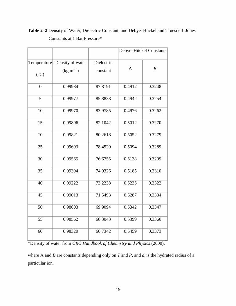
Table 2–2 Density of Water, Dielectric Constant, and Debye–Hückel and Truesdell–Jones

Constants at 1 Bar Pressure*

Debye–Hückel Constants

Temperature

(°C)

Density of water

(kg m– 3

)

Dielectric

constant A B

0 0.99984 87.8191 0.4912 0.3248

5 0.99977 85.8838 0.4942 0.3254

10 0.99970 83.9785 0.4976 0.3262

15 0.99896 82.1042 0.5012 0.3270

20 0.99821 80.2618 0.5052 0.3279

25 0.99693 78.4520 0.5094 0.3289

30 0.99565 76.6755 0.5138 0.3299

35 0.99394 74.9326 0.5185 0.3310

40 0.99222 73.2238 0.5235 0.3322

45 0.99013 71.5493 0.5287 0.3334

50 0.98803 69.9094 0.5342 0.3347

55 0.98562 68.3043 0.5399 0.3360

60 0.98320 66.7342 0.5459 0.3373

*Density of water from CRC Handbook of Chemistry and Physics (2000).

where A and B are constants depending only on T and P, and ai is the hydrated radius of a

particular ion.

20

At atmospheric pressure,

1.56 0.5

01.824928 10A T

and B = 50.3(εT)

–0·5, where ρ0 is the

density of water, ε is the dielectric constant of water, and T is in Kelvin. At any temperature T (in

the range 0° to 100°C), the dielectric constant can be determined from the following relationship:

ε = 2727.586 + 0.6224107T – 466.9151 ln T – 52000.87/T (2–42)

where T is in Kelvin. At 25°C, ρ0 = 0.99693, ε = 78.4520, A = 0.5094, and B = 0.3289. Values for

the density of water, the dielectric constant of water, and the A and B Debye–Hückel constants at 1

bar, from 0° to 60°C, are tabulated in Table 2–2.

A word of caution. Compilations of the hydrated radii of ions (ai) tend to use different units. If the

radii are given directly in angstroms, then the value for B can be used as calculated (or as given in

Table 2–2). If the radii are tabulated as 10–10

m or 10–8

cm, then B must be multiplied by 1010 or 10

8,

respectively.

Truesdell–Jones Model

The Truesdell–Jones (Truesdell and Jones, 1974) and Davies (Davies, 1962) equations are

extended versions of the Debye–Hückel equation. An additional term is added to the Debye–

Hückel equation that takes into account the observation that in high-ionic-strength experimental

systems the activity coefficients begin to increase with increasing ionic strength. The Truesdell–

Jones equation is written

2

log1

ii

i

Az IbI

Ba I

(2–43)

where ai and b are determined from experimental data. Because the ai values are determined

experimentally—i.e., they are selected so that the calculated curves fit the observed data—these ai

values can only be used in the Truesdell–Jones equation (2–43). The A and B constants are the

same in both the Truesdell–Jones and Debye–Hückel equations. Selected values for Debye–

Hückel ai and Truesdell–Jones ai and b are given in Table 2–3.

21

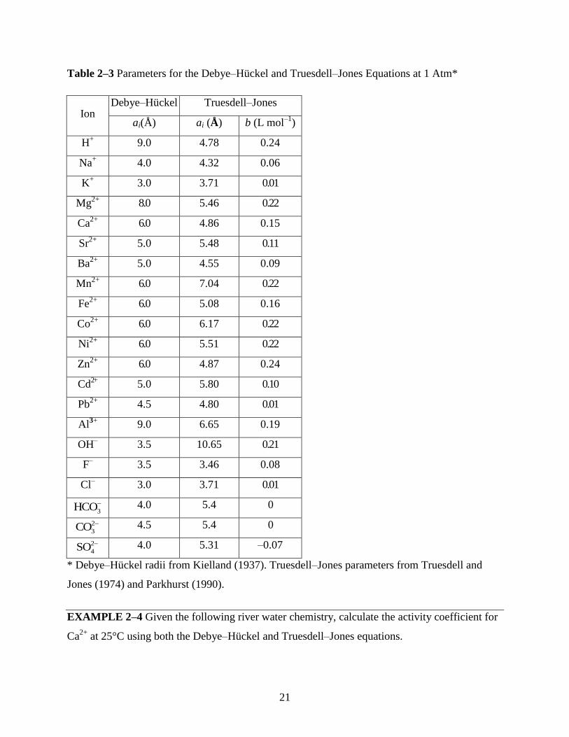
Table 2–3 Parameters for the Debye–Hückel and Truesdell–Jones Equations at 1 Atm*

Ion Debye–Hückel Truesdell–Jones

ai(Å) ai (Å) b (L mol–1

)

H+ 9.0 4.78 0.24

Na+ 4.0 4.32 0.06

K+ 3.0 3.71 0.01

Mg2+

8.0 5.46 0.22

Ca2+

6.0 4.86 0.15

Sr2+

5.0 5.48 0.11

Ba2+

5.0 4.55 0.09

Mn2+

6.0 7.04 0.22

Fe2+

6.0 5.08 0.16

Co2+

6.0 6.17 0.22

Ni2+

6.0 5.51 0.22

Zn2+

6.0 4.87 0.24

Cd2+

5.0 5.80 0.10

Pb2+

4.5 4.80 0.01

Al3+

9.0 6.65 0.19

OH– 3.5 10.65 0.21

F– 3.5 3.46 0.08

Cl– 3.0 3.71 0.01

3HCO

4.0 5.4 0

2

3CO

4.5 5.4 0

2

4SO

4.0 5.31 –0.07

* Debye–Hückel radii from Kielland (1937). Truesdell–Jones parameters from Truesdell and

Jones (1974) and Parkhurst (1990).

EXAMPLE 2–4 Given the following river water chemistry, calculate the activity coefficient for

Ca2+

at 25°C using both the Debye–Hückel and Truesdell–Jones equations.

22

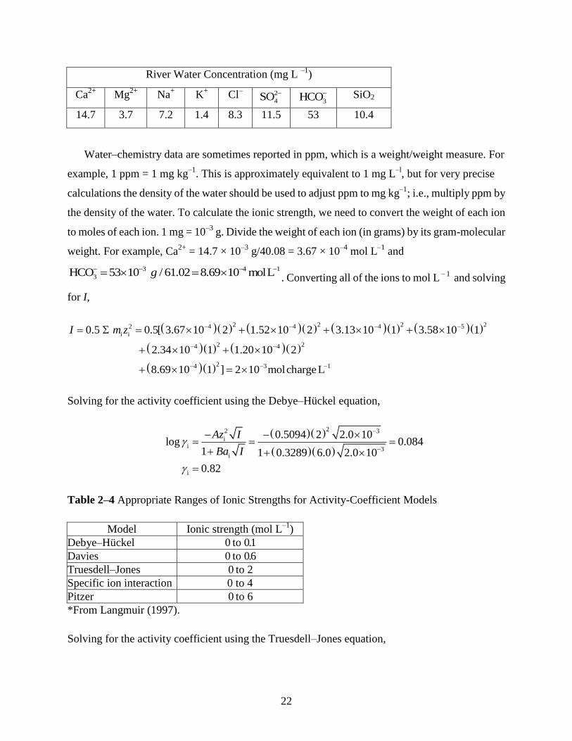
River Water Concentration (mg L –1

)

Ca2+

Mg2+

Na+ K

+ Cl

– 2

4SO

3HCO

SiO2

14.7 3.7 7.2 1.4 8.3 11.5 53 10.4

Water–chemistry data are sometimes reported in ppm, which is a weight/weight measure. For

example, 1 ppm = 1 mg kg–1

. This is approximately equivalent to 1 mg L–l

, but for very precise

calculations the density of the water should be used to adjust ppm to mg kg–1

; i.e., multiply ppm by

the density of the water. To calculate the ionic strength, we need to convert the weight of each ion

to moles of each ion. 1 mg = 10–3

g. Divide the weight of each ion (in grams) by its gram-molecular

weight. For example, Ca2+

= 14.7 × 10–3

g/40.08 = 3.67 × 10–4

mol L–1

and

3 4 1

3HCO 53 10 / 61.02 8.69 10 molLg . Converting all of the ions to mol L

– 1 and solving

for I,

2 2 2 22 4 4 4 5

i i

2 24 4

24 3 1

0.5 0.5[ 3.67 10 2 1.52 10 2 3.13 10 1 3.58 10 1

2.34 10 1 1.20 10 2

8.69 10 1 ] 2 10 molchargeL

I m z

Solving for the activity coefficient using the Debye–Hückel equation,

22 3

ii

3i

i

0.5094 2 2.0 10log 0.084

1 1 0.3289 6.0 2.0 10

0.82

Az I

Ba I

Table 2–4 Appropriate Ranges of Ionic Strengths for Activity-Coefficient Models

Model Ionic strength (mol L–1

)

Debye–Hückel 0 to 0.1

Davies 0 to 0.6

Truesdell–Jones 0 to 2

Specific ion interaction 0 to 4

Pitzer 0 to 6

*From Langmuir (1997).

Solving for the activity coefficient using the Truesdell–Jones equation,

23

2

ii

i

2 33

3

log1

0.5094 2 2.0 100.15 2.0 10 0.085

1 0.3289 4.86 2.0 10

Az IbI

Ba I

At concentrations typical of river water, both models yield essentially the same activity

coefficient, and hence either model could be used to calculate the activity coefficients for river and

lake waters with low ionic strength. The useable range of ionic strengths for each model is

tabulated in Table 2–4.

Pitzer Model

For solutions of higher ionic strength, the Pitzer model would be most appropriate. The Pitzer

model (Pitzer, 1973, 1979, 1980) takes into account binary interactions between two ions of the

same or opposite sign and ternary interactions between three or more ions. This model is most

effective for concentrated brines. The solutions are generally complex and best carried out by

computer. Further details on the Pitzer model can be found in Langmuir (1997). Several of the

commonly used water-chemistry computer codes (SOLMINEQ.88, PHRQPITZ, and PRHEEQC)

use the Pitzer model.

Why Do We Care About Activity-Coefficient Models?

The preceding has not been an exhaustive discussion of activity coefficient calculations for ionic

species, but it has drawn attention to the types of models and the limitations of the models. A

number of computer codes have been developed to calculate speciation in natural waters. These

different programs use different activity-coefficient models. The user should be aware of these

differences. For example, it would be inappropriate to do speciation calculations for a brine using a

computer code based on the Debye–Hückel model. The user should select a computer model

appropriate for the system being considered. Table 2–4 summarizes the range of ionic strengths

appropriate for each activity-coefficient model.

Calculation of Activity Coefficients for Uncharged Species

There are several activity-coefficient models for uncharged species. Plummer and MacKenzie

24

(1974) calculate the activity coefficient (γ) for an uncharged species as follows:

γ = 100.11

(2–44)

where I is the ionic strength. The empirical Setchenow equation (Millero and Schreiber, 1982)

calculates γ as follows:

log γi = K iI (2–45)

where Ki is a constant ranging in value from 0.02 to 0.23 at 25°C. For relatively dilute aqueous

systems, such as rivers and lakes, which have ionic strengths on the order of 2 × 10–3

, and brackish

waters with ionic strengths on the order of 2 × 10–2

, both equations give activity coefficients close

to 1. For concentrated solutions, such as seawater, the activity coefficient is greater than 1.

Seawater has an ionic strength of about 0.7, which, using the Plummer and MacKenzie (1974)

model, yields an activity coefficient of 1.17. Values calculated from the Setchenow equation will

vary as a function of the uncharged species. For example, the Ki value for H4SiO4 (aq) at 25°C is

0.080 (Marshall and Chen, 1982), giving a calculated activity of 1.14 for this uncharged species.

An important point is that with increasing ionic strength, compounds that yield uncharged species

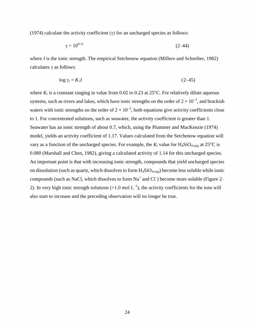
on dissolution (such as quartz, which dissolves to form H4SiO4 (aq)) become less soluble while ionic

compounds (such as NaCl, which dissolves to form Na+ and Cl

–) become more soluble (Figure 2–

2). In very high ionic strength solutions (>1.0 mol L–1

), the activity coefficients for the ions will

also start to increase and the preceding observation will no longer be true.

25

Figure 2-2 Schematic representation of the variation in activity coefficients versus the ionic

strength of solutions.

Activity of Water

When water is a solvent, pure liquid water at infinite dilution is used as the standard state; i.e., the

activity of H2O = 1 at infinite dilution. The activity of water is related to the mole fraction of pure

water, 2H OXas follows:

2 2 2

0

H O H O H OlnRT X (2–46)

In most cases, we are dealing with dilute solutions and we can set the activity of H2O = 1. In more

concentrated solutions, such as seawater, the activity will be slightly less than 1.

AQUEOUS COMPLEXES

An aqueous complex is a dissolved species formed from two or more simpler species, each of

which can exist in aqueous solution (Drever, 1997, p. 34). In the context of equilibrium

calculations, complexes are important because their formation can increase the solubility of

various compounds. Consider the following reaction:

26

A+ + B

– ⇌ AB (aq) (2–47)

We can write an equilibrium equation for this reaction in the usual way. In this case, the

equilibrium constant is called a stability constant because it is a measure of the stability of the

aqueous complex.

aq

stab

AB

A BK

(2–48)

The solubility of compounds whose ions form aqueous species is increased over that predicted

from the solubility product for the compound. This is because some of the ions released during the

dissolution process are taken up by the aqueous complex. For a solution at saturation, the

concentration of the aqueous complex can be determined from

[AB(aq)] = Kstab · [A+][B–] = Kstab Ksp (2–49)

Setting the activity of the solid equal to 1, Ksp = [A+][B

–]. Since the aqueous complex is an

uncharged species, at low to moderate ionic strengths the activity coefficient is 1, and

concentration equals activity.

EXAMPLE 2–5 In pure water the solubility of gypsum is 10.2 × 10–3

mol L–1

. Calcium and sulfate

ions in solution form an aqueous complex according to the following reaction:

2 2

4 4 aqCa SO CaSO

4 aq 2.23

stab 2 2

4

CaSO10

Ca SOK

2 2

stab 4 stab4 aq sp gypsum

2.23 4.60 2.37 3

CaSO Ca SO

10 10 10 4.3 10

K K K

The activity coefficient for an uncharged species is approximately 1. Therefore, the activity and

concentration of the uncharged species is the same. Given that the concentration of CaSO4 (aq) is

4.3 × 10–3

mol L–1

, the solubility of gypsum in pure water has increased from 10.2 × 10–3

mol L–1

to

27

14.5 × 10–3

mol L–1

an increase in solubility of approximately 40% due to the formation of the

aqueous complex.

Some elements occur in solution predominantly as complexes rather than free ions. For these

elements it is the properties of the complexes rather than the free ions that determine their behavior

in natural systems. Certain metals become soluble when the opportunity arises to form a particular

type of aqueous complex. For example, Fe3+

and Al3+

are generally immobile in the weathering

environment. However, in the presence of oxalic acid (H2C2O4) these ions can become mobile.

Oxalic acid dissociates to form H+ and COO

– (an oxalate ion). This ion can bond to a metal,

forming a complex species. The anion is a ligand (an anion or neutral molecule that can combine

with a cation). Given the abundance of dissolved organic matter in the natural environment, this

type of aqueous complex can be important in the transport of iron and aluminum.

Ligands can be either monodentate (one pair of shared electrons in a complex) or multidentate

(more than one pair of shared electrons in a complex). Inorganic ligands tend to form monodentate

complexes, and organic ligands tend to form multidentate complexes. The maximum number of

ligands that can bond to a single cation is a function of the relative size of the cation and ligand (see

Chapter 7 for a discussion of coordination). In natural waters the number of potential ligands is

usually too low for this maximum number to be achieved. Ligands that form multiple bonds with a

cation and have a “cagelike” structure are referred to as chelates. The metal cation is strongly

bonded in these types of structures and chelation is an important process for the removal of metals

from the aqueous environment.

MEASUREMENT OF DISEQUILIBRIUM

We have now considered the thermodynamic basis of equilibrium calculations. A remaining

question is, How do we measure how close a particular reaction is to equilibrium? Consider the

dissolution of gypsum:

2+ 2

4 2 gypsum 4 2CaSO 2H O Ca SO 2H O

The solubility product for this reaction is written

28

2 2 4.60

sp 4Ca SO 10K

If the system is at equilibrium, the concentration of species in solution (Activity Product [AP] if

both ions and uncharged species are involved; Ion Activity Product [IAP] if only charged species

are involved) will equal the solubility product. In this example we are dealing with ions, so at

equilibrium IAP = 10–4.60

(the Ksp for gypsum). If the IAP is less than 10–4.60

, the solution is

undersaturated with respect to gypsum; and if the IAP is greater than 10–4.60

, the solution is

supersaturated with respect to gypsum. Quantitatively, the approach to equilibrium can be

expressed as AP (or IAP)/Ksp, which is 1 at equilibrium, or log [AP (or IAP)/Ksp], which is 0 at

equilibrium.

EXAMPLE 2–6 In a particular solution [Ca2+

] = 10–3

mol L–l

and 2

4SO . At 25°C, is the

solution over-or undersaturated with respect to gypsum? Give a quantitative measure of the degree

of over-or undersaturation.

3 20.40

4.60

sp

IAP 10 1010

10K

IAP/Ksp is less than 1 so the solution is undersaturated with respect to gypsum.

KINETICS

Equilibrium thermodynamics predicts the final state of the system. Kinetics tells us if the system

will actually achieve this state within a reasonable time. In practice, the determination of rates of

reaction is not a straightforward exercise. A number of factors affect these rates, and careful

experimentation is required to understand the reaction mechanisms. Consider, for example, the

dissolution of gypsum in water.

2+ 2

4 2 gypsum 4 2CaSO 2H O Ca SO 2H O

This reaction involves several steps. First, the ions need to be freed from the crystal structure, and

then they need to be transported away from the crystal surface. The first step requires an energy

input to break the bonds in the crystal structure, and the second step is diffusion controlled. The

29

importance of the second step may not be obvious, but consider what will happen if the Ca2+

and

2

4SO

ions are not removed from the immediate vicinity of the gypsum crystal. The concentration

of the ions in solution will increase until the microenvironment surrounding the gypsum crystal

becomes saturated with respect to gypsum. At this point the dissolution will stop. Whichever of

these steps is the slowest will determine the rate at which the dissolution reaction proceeds. As

another example, from metamorphic petrology, consider the apparently simple phase transition

sillimanite ⇌ kyanite. Sillimanite and kyanite are polymorphs of Al2SiO5, and the reaction

suggests that sillimanite is directly converted to kyanite through the rearrangement of atoms in the

crystal structure. Petrographic investigations, however, suggest that this is a much more complex

reaction, in which the sillimanite first breaks down to form other minerals and is then reformed as

kyanite. Hence, what appears to be a very simple reaction actually involves several steps. The

slowest of these steps would determine the rate for the overall reaction.

Reactions are of two types: homogeneous and heterogeneous. Homogeneous reactions only

involve one phase (gas, liquid, or solid). Heterogeneous reactions involve two or more phases.

Consider the condensation of water vapor in the atmosphere. If the condensation process involves

water vapor condensing directly from the vapor phase, the reaction is homogeneous (it occurs in

the gas phase). If the water vapor condenses onto a particle, the reaction is heterogeneous (a gas

and a solid are involved). Direct nucleation turns out to be difficult, and in the homogeneous

system significant supersaturation is required before condensation actually occurs. On the other

hand, the presence of particles facilitates nucleation and in the heterogeneous system condensation

occurs close to saturation. Another example from everyday experience is the crystallization of

“rock candy.” In practice, this is done by heating water on a stove and dissolving copious amounts

of sugar in the water. The water is then slowly cooled to room temperature, and the system is now

significantly supersaturated with respect to sugar. A small sugar crystal is introduced into the

water and serves as a site of nucleation. Rapid crystal growth occurs as the sugar in the

supersaturated system precipitates onto the sugar crystal. Virtually all reactions of interest in

nature are heterogeneous, but the best understood reactions in terms of kinetics are homogeneous,

a not unusual situation in science.

30

Order of Reactions

For an elementary reaction, the order is defined by the number of individual atoms or molecules

involved in the reaction. We can talk about order in terms of an individual species or in terms of the

overall reaction. Consider the reaction A + B → AB. The reaction is first order in terms of A and B

and the overall reaction is second order. The reaction A + 2B → C is first order with respect to A

and C, second order with respect to B, and third order overall. Differential and integrated equations

follow for the different types of reactions. Also listed is the equation for the half-life (t1/2) of each

type of reaction—i.e., the time it will take for half of the reactant to be consumed in the reaction.

Zeroth order. The reaction rate is independent of the concentration of the reactant (A).

00 1/2

0.5AA, A A ,

dk kt t

dt k

(2–50)

First order. The reaction rate is dependent on the concentration of the reactant, A→ B.

0 1/2

A 0.693A, lnA lnA ,

dk kt t

dt k

(2–51)

The first-order rate equations may look familiar since radioactive decay is a first-order

reaction—t1/2 in this case being the half-life of the radioactive parent.

Second order. The reaction rate is dependent on the concentration of the reactant, 2A → B.

2

1/2

0 0

A 1 1 1A , ,

A A A

dk kt t

dt k

(2–52)

Note that the units for k depend on the order of the reaction. For example, zeroth-order

reaction, mol cm–1

s–1

; first-order, s–1

, and second-order, cm3 mol

–1 s

–1. Higher-order reactions are

possible, but in most geochemical systems of interest the reactions are second order or less. The

order of a reaction can be determined by experiment. For example, if the reaction is zeroth order,

an arithmetic plot of concentration versus time will yield a straight line. If the reaction is first

order, an arithmetic plot of concentration versus time will yield a curved line, because for a

first-order reaction the relationship between concentration and time is exponential. A log-log plot

of the rate of the reaction versus concentration will yield a straight line whose slope defines the

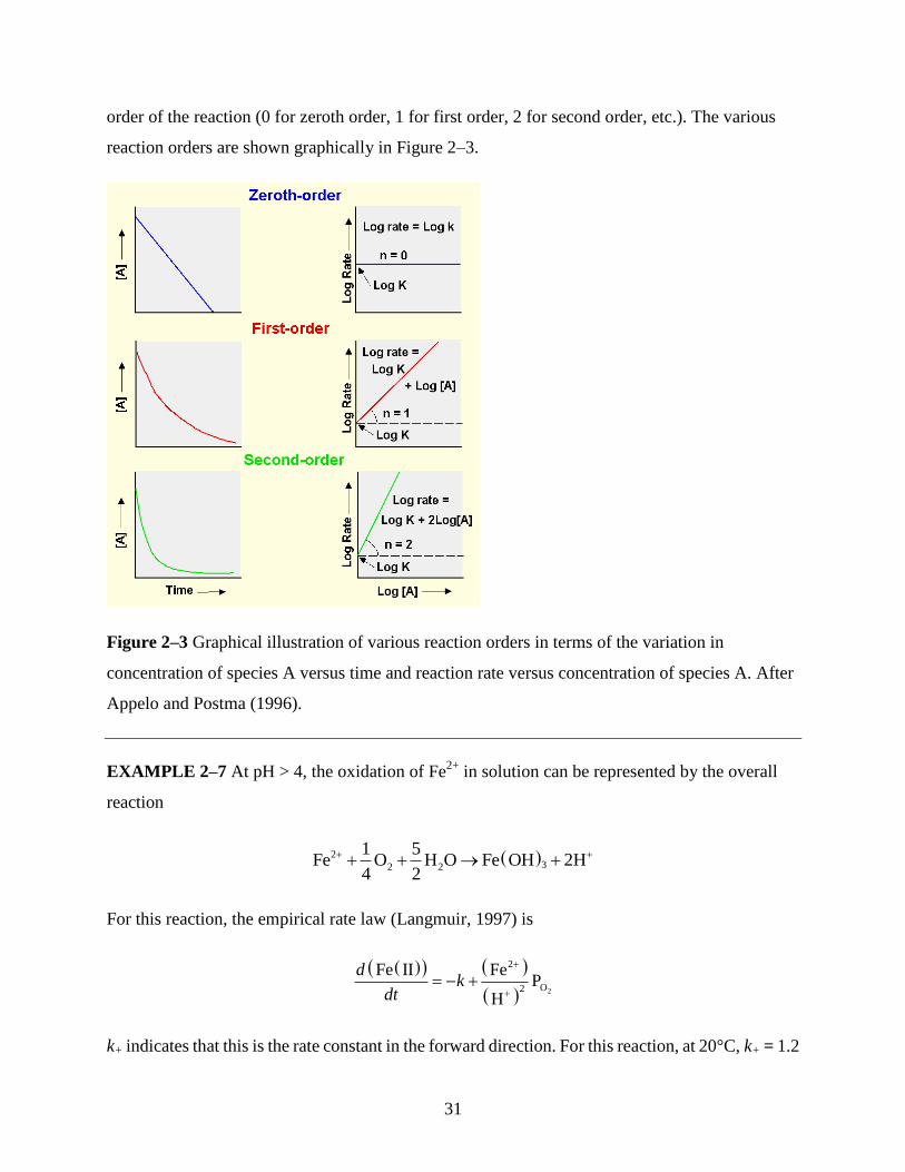
31

order of the reaction (0 for zeroth order, 1 for first order, 2 for second order, etc.). The various

reaction orders are shown graphically in Figure 2–3.

Figure 2–3 Graphical illustration of various reaction orders in terms of the variation in

concentration of species A versus time and reaction rate versus concentration of species A. After

Appelo and Postma (1996).

EXAMPLE 2–7 At pH > 4, the oxidation of Fe2+

in solution can be represented by the overall

reaction

232 2

1 5Fe O H O Fe OH 2H

4 2

For this reaction, the empirical rate law (Langmuir, 1997) is

2

2

O2

Fe II FeP

H

dk

dt

k+ indicates that this is the rate constant in the forward direction. For this reaction, at 20°C, k+ = 1.2

32

× 10–11

mol2 bar

–1 d

–1. Under atmospheric conditions,

2OP 0.2 bar. Given that Fe2+

in solution =

1 × 10–3

mol L–1

, calculate the reaction rate at pH = 5 and pH = 7.

At pH = 5,

2

2 311 5 1 1

O2 25

Fe 1 10Rate P 1.2 10 0.2 2.4 10 molL d

H 10k

At pH = 7,

2

2 311

O2 27

1 1 1

Fe 1 10Rate P 1.2 10 0.2

H 10

2.4 10 molL d

k

The reaction rate increases by 4 orders of magnitude in going from pH = 5 to pH = 7.

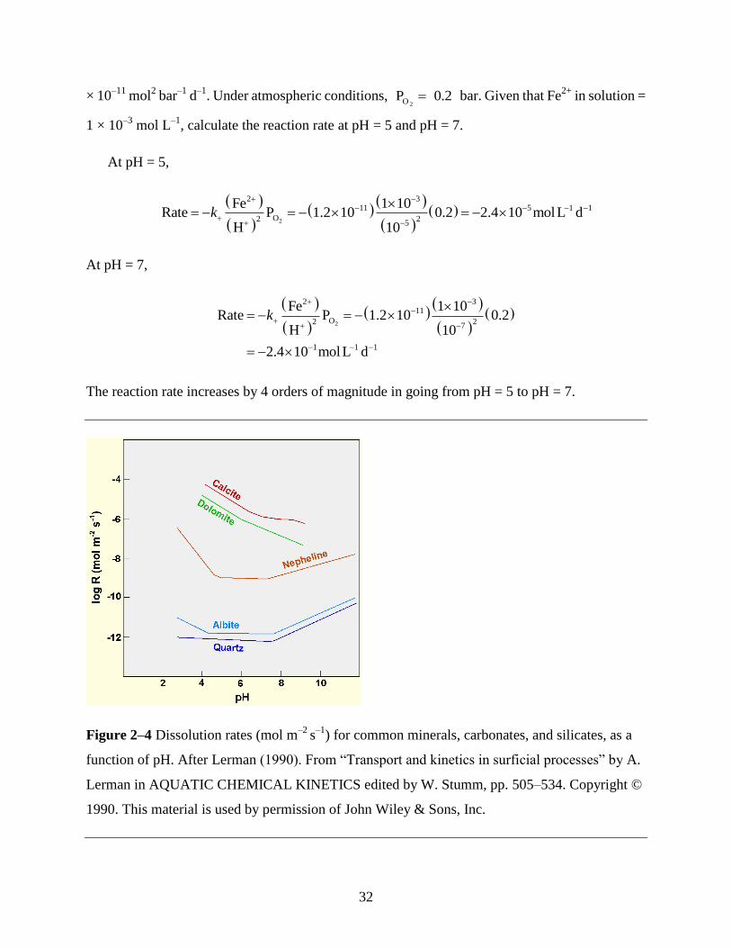
Figure 2–4 Dissolution rates (mol m–2

s–1

) for common minerals, carbonates, and silicates, as a

function of pH. After Lerman (1990). From “Transport and kinetics in surficial processes” by A.

Lerman in AQUATIC CHEMICAL KINETICS edited by W. Stumm, pp. 505–534. Copyright ©

1990. This material is used by permission of John Wiley & Sons, Inc.

33

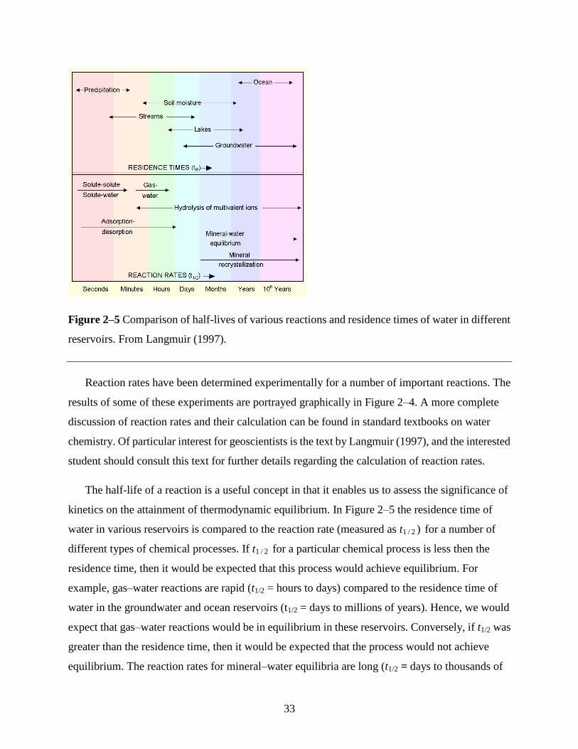
Figure 2–5 Comparison of half-lives of various reactions and residence times of water in different

reservoirs. From Langmuir (1997).

Reaction rates have been determined experimentally for a number of important reactions. The

results of some of these experiments are portrayed graphically in Figure 2–4. A more complete

discussion of reaction rates and their calculation can be found in standard textbooks on water

chemistry. Of particular interest for geoscientists is the text by Langmuir (1997), and the interested

student should consult this text for further details regarding the calculation of reaction rates.

The half-life of a reaction is a useful concept in that it enables us to assess the significance of

kinetics on the attainment of thermodynamic equilibrium. In Figure 2–5 the residence time of

water in various reservoirs is compared to the reaction rate (measured as t1 / 2 ) for a number of

different types of chemical processes. If t1 / 2 for a particular chemical process is less then the

residence time, then it would be expected that this process would achieve equilibrium. For

example, gas–water reactions are rapid (t1/2 = hours to days) compared to the residence time of

water in the groundwater and ocean reservoirs (t1/2 = days to millions of years). Hence, we would

expect that gas–water reactions would be in equilibrium in these reservoirs. Conversely, if t1/2 was

greater than the residence time, then it would be expected that the process would not achieve

equilibrium. The reaction rates for mineral–water equilibria are long (t1/2 = days to thousands of

34

years) compared to the residence time for precipitation in the atmosphere (t1 / 2 = seconds to hours).

Hence, in atmospheric aerosols we would not expect solid particles and the liquid or vapor phase

to be in equilibrium.

The Arrhenius Equation

The Arrhenius equation relates the rate at which a reaction occurs to the temperature:

exp aEk A

RT

(2–53)

where A is a pre-exponential factor generally determined by experiment and relatively

independent of temperature, Ea is the activation energy for the reaction, R is the ideal gas constant,

and T is the temperature in Kelvin. Converting to base 10 logs gives

log log2.303

aEk A

RT

(2–54)

Activation energies are determined by experiment. If a particular reaction follows the Arrhenius

relationship, then a plot of log k versus 1/T yields a straight line with a slope of –Ea/2.303R. A

rough rule of thumb is that the reaction rate doubles with every 10°C increase in temperature.

Measured activation energies (in kJ mol–1

) vary from 8 to 500 depending on the process. Simple

physical adsorption has low activation energies, and solid phase reactions (such as solid-state

diffusion) have high activation energies.

EXAMPLE 2–8 One of the reactions in the carbonate system is

2

3 calcite 2 33 aqCaCO H CO Ca 2HCO

For this reaction, the rate constant at 25°C is 3.47 × 10–5

s–1

and log k = –4.46. Determine the value

of the pre-exponential term A for this reaction and determine the rate constant for the reaction at

10°C.

The activation energy for the reaction is 41.85 kJ mol–1

. First determine the preexponential

factor by rearranging equation 2–54 to solve for log A.

35

1

a

3 1 1

41.85 kJ mollog log 4.46

2.303 2.303 8.314 10 kJ mol K 298.15K

4.46 7.33 2.87

EA k

RT

Calculate the reaction rate constant at 10°C using equation 2–54.

1

a

3 1 1

41.85 kJ mollog log 2.87

2.303 2.303 8.314 10 kJ mol K 283.15K

2.87 7.72 4.85

Ek A

RT

and k = 1.41 × 10–5

s–1

. Changing the temperature from 25°C to 10°C leads to an approximately

2.5X decrease in the reaction rate.

Nucleation

There are two types of nucleation—homogeneous and heterogeneous. Homogeneous nucleation

occurs when a nucleus forms spontaneously in an oversaturated solution.

Heterogeneous nucleation occurs when a nucleus forms in contact with a, usually solid, surface.

Homogeneous nucleation requires a much greater degree of supersaturation than heterogeneous

nucleation.

The free energy of formation of a nucleus consists of the energy gained from the formation of

bonds and the energy required to create the surface. This can be written mathematically as

∆Gnuc = ∆Gbulk + ∆Gsurf (2–55)

For an oversaturated solution, ∆Gbulk is always negative. For ∆Gbulk, we can write the following

equation:

3

bulk

0

4ln

3B

r aG k T

V a

(2–56)

where 4πr3/3V is the volume of a spherical nucleus, V is the molecular volume, kB is the

Boltzmann constant (1.3805 × 10–23

J K–1

), T is the temperature in Kelvin, a is actual activity, and

a0 is the activity for a saturated solution.

36

For ∆Gsurf, we can write

2

surf 4G r (2–57)

where is the interfacial energy. Interfacial energies vary over several orders of magnitude. For

example, amorphous silica has a surface free energy of 46 × 10–3

J m–2

and goethite has a surface

free energy of 1600 × 10–3

J m–2

. Combining equations 2–56 and 2–57 yields

32

nuc

0

4ln 4

3B

r aG k T r

V a

(2–58)

From equation 2–58 it is obvious that increasing the degree of oversaturation favors

nucleation, as does increasing the radius of the particle. For any particular particle size and degree

of oversaturation the ease of nucleation is a function of the interfacial energy; e.g., from the data

just given it is much more difficult to nucleate goethite than amorphous silica. The rate at which

nuclei form can be determined from the standard Arrhenius rate equation,

*Rateof nucleation= exp

B

GA

k T

(2–59)

where Ā is a factor related to the efficiency of collisions of ions or molecules, ∆G* is the

maximum energy barrier (see Figure 2–6), kB is the Boltzmann constant, and T is the temperature

in Kelvin.

Interfacial energies are different for nuclei formed via homogeneous reactions versus nuclei

formed via heterogeneous reactions. A discussion of this difference can be found in standard

water-chemistry books, such as Stumm and Morgan (1996).

37

Figure 2–6 Variation of free energy of nucleation as a function of particle radius. The maximum

free energy of formation corresponds to the maximum energy barrier. At greater particle radii the

free energy of nucleation decreases and eventually becomes negative, and nucleation will proceed

spontaneously. Modified from Drever (1997).

Dissolution and Growth

Once a nucleus has formed, the next question is, how fast will the particle grow? This is a function

of several factors: (1) the rate at which the ions (or complex molecules) diffuse through the liquid

to the surface of the growing particle and (2) the rate at which the ions or molecules are attached to

the surface of the growing particle. One of these will be the rate-limiting step. In addition, during

dissolution of a particle, there may be a reaction zone between the surface of the original grain and

the solution. For example, feldspars break down by incongruent dissolution (the feldspar

decomposes to a mineral of different composition and species that enter the solution). Thus, a

feldspar grain may become coated with a rim of reaction product through which the ions must

diffuse in order for the reaction to continue. As the thickness of this reaction rim increases, the

diffusion of ions or molecules through the reaction zone may become the rate-limiting step (Figure

2–7).

38

Figure 2–7 Schematic representation of a mineral reacting with a solution during dissolution. The

rate-controlling step can be the diffusion of species through the solution, diffusion of species

through the reaction zone, or the rate of the surface reaction. Given the slow rate of diffusion of

species through the reaction zone, at some point the thickness of this zone will become sufficiently

great that the diffusion of species through the reaction zone will become the rate controlling step.

Modified from Drever (1997).

The topology of the mineral surface is also important in determining the rate at which both

dissolution and particle growth occur. The mineral surface is usually not planar, but consists of

steps and kinks. Atoms that form steps and kinks have higher energy, and dissolution or growth

takes place at these locations. Dislocations occur when one part of a crystal Structure is offset

relative to another part. The number and types of dislocations are important in determining the

rate of dissolution or growth. Inhibitors, or surface poisons, are foreign species adsorbed at

points of high energy on the crystal surface that may inhibit crystal growth or dissolution. For

example, in seawater the concentration of phosphate ions affects the dissolution rate of calcite. It is

believed that the phosphate ion acts as an inhibitor and is preferentially attached to sites of high

energy on the crystal surface.

WATER-CHEMISTRY COMPUTER MODELS

The previous discussion of thermodynamics and kinetics has been far from exhaustive but was

39

intended to introduce the basic concepts used in the modeling of water chemistry. Because these

calculations can be very laborious, a number of computer models have been developed to do these

types of computations. These computer models can be divided into three basic types: speciation,

mass transfer, and chemical mass transport. Speciation models calculate the partitioning of

elements between aqueous species and determine the degree of saturation with respect to mineral

and gas phases. The calculations that we considered in the section on equilibrium thermodynamics

were of this type. The U.S. Geological Survey’s WATEQ4F is an example of this type of model.

Mass transfer models do the same types of calculations as speciation models but in addition

consider the effect of mass transfer processes (dissolution, precipitation, gas exchange, ion

exchange, adsorption, etc.). Examples of these types of models are PHREEQC and PHRQPITZ

(U.S. Geological Survey). Chemical mass transport models include speciation, mass transfer

processes, and hydrodynamic advection and dispersion. An example of this type of model is the

U.S. Geological Survey’s PHREEQM-2D.

The major sources of free computer models are the U.S. Environmental Protection Agency and

the U.S. Geological Survey. These models can be accessed from the appropriate agency’s web

pages. The addresses listed here are current at the time of publication, but the various agencies do

occasionally change their web addresses.

The site for the U.S. Environmental Protection Agency software is

http://www.epa.gov/epahome/models.htm. The programs are developed and maintained by the

Center for Exposure Assessment Modeling (CEAM). These are DOS-based programs, and a

number of different types are available. The water-chemistry model is MINTEQA2, which can be

used to calculate the equilibrium compositions of dilute solutions.

The site for the U.S. Geological Survey software is http://water.usgs.gov/software. Most of

the programs can be run on UNIX or DOS platforms. Windows versions are available for some of

the programs. One of the problems with USGS software is that it has not been very user-friendly.

This problem has been addressed through the development of CHEMFORM, which serves as an

interface for the various programs. Included in the program inventory are mass balance models

(NETPATH), speciation models (WATEQ4F) and mass transfer models (PHREEQC,

PHREEQCI, PHRQPITZ). Besides water-chemistry models, a number of other hydrological

models are available at this site.

40

Another site of interest, not only in terms of water-chemistry models but also in terms of

geochemical data and analysis in general, is the Geochemical Earth Reference Model (GERM).

The address for GERM is http://earthref.org/GERM/main.htm. This site not only provides

links to a number of water-chemistry models but also has tabulations of thermodynamic data,

information on elemental abundances in various reservoirs, and a number of other useful

tabulations. The site is under continual development and over time should become a major source

of geochemical and environmental data. The Geochemical Society, http://gs.wustl.edu, also has

links to sites that provide geochemical data. This site, presumably, will also expand with time and

the number of linkages will increase.

Among the commercially available software, the most powerful and widely used is the

Geochemist’s Workbench (Bethke, 1996). This set of computer models was originally developed

at the University of Illinois and consists of a number of modules that can be used to carry out

calculations involving speciation, plotting of stability diagrams, reaction paths, and a variety of

mass transfer processes.

Only a few of the models include kinetics, and a variety of activity-coefficient models are used.

The user should consult the documentation that comes with each computer code to determine how

that particular code does the computations. Particular attention should be paid to the

activity-coefficient models (i.e., are they appropriate for the problem?) and the thermodynamic

database. Further information on computer models can be found in Mangold and Tsang (1991),

van der Heijde and Elnawawy (1993), and Langmuir (1997).

CASE STUDIES

The following three case studies show how water-chemistry computer models can be applied to

environmental problems. The Case Study 2–1 considers the impact of acid mine drainage on the

downstream quality of a watercourse. The author of the study used geochemical modeling to

determine the chemical processes affecting the concentration of each species of interest. The

author was also able to determine the first-order rate constant for the removal of iron from the

stream. Such calculations are of interest because they tell us how far a particular contaminant will

be transported by a river system.

In Case Study 2–2, the authors used several ionic species as tracers to determine the relative

41

percentage of leachate from a municipal landfill sited on an aquifer. One of the species was found

to behave conservatively, and the other was found to show nonconservative behavior when there

was a significant leachate component in the aquifer.

In Case Study 2–3, the author investigated the impact of acid deposition on ground-water

quality and concluded that the system was not well buffered against acid additions. Increased

acidity might result in the release of trace metals, tied up in clay minerals, to the groundwater

system.

CASE STUDY 2–1

Geochemical Modeling of Coal Mine Drainage, Summit County, Ohio

A serious problem associated with coal mining is the generation of acid mine drainage (AMD).

During mining, sulfur-bearing minerals, such as pyrite (FeS2), are exposed to oxygen and water,

leading to a series of oxidation and hydrolysis reactions that produce sulfuric acid. The resulting

waters are strongly acidic (pH of 2 or less is possible) and have high concentrations of 2

4SO

, Fe2+

,

Al3+

, and Mn2+

. Such waters are toxic to aquatic life and vegetation.

Foos (1997) investigated the downstream changes in the chemistry of coal mine drainage at

Silver Creek Metropark, Summit County, Ohio. The first step was to construct a simple mixing

model in which AMD and water discharged from Silver Creek lake were the end members. This

model successfully predicted the concentrations of Cl–,

3

4PO

, Ca2+

, Mg2+

and Na+, indicating that

these species behaved conservatively; i.e., they were not reacting with their surroundings.

However, the model did not accurately predict the concentrations of 3HCO

, 2

4SO

, Fe3+

, Mn2+

,

and Si. The model underestimated the concentration of 3HCO

, indicating that this species was

being added to the system, and overestimated the concentrations of the other four species,

indicating that they were being removed from the system. Sampling along the length of the

discharge stream showed a downstream increase in 3HCO

and a downstream decrease in the

other four species. There was an excellent correlation between Fe2+

concentration and distance.

42

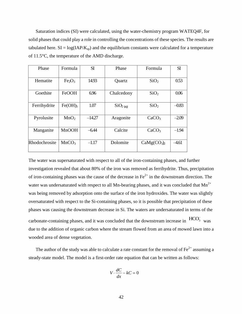
Saturation indices (SI) were calculated, using the water-chemistry program WATEQ4F, for

solid phases that could play a role in controlling the concentrations of these species. The results are

tabulated here. SI = log(IAP/Ksp) and the equilibrium constants were calculated for a temperature

of 11.5°C, the temperature of the AMD discharge.

Phase Formula SI Phase Formula SI

Hematite Fe2O3 14.93 Quartz SiO2 0.53

Goethite FeOOH 6.96 Chalcedony SiO2 0.06

Ferrihydrite Fe(OH)3 1.07 SiO2 (aq) SiO2 –0.83

Pyrolusite MnO2 –14.27 Aragonite CaCO3 –2.09

Manganite MnOOH –6.44 Calcite CaCO3 –1.94

Rhodochrosite MnCO3 –1.17 Dolomite CaMg(CO3)2 –4.61

The water was supersaturated with respect to all of the iron-containing phases, and further

investigation revealed that about 80% of the iron was removed as ferrihydrite. Thus, precipitation

of iron-containing phases was the cause of the decrease in Fe2+

in the downstream direction. The

water was undersaturated with respect to all Mn-bearing phases, and it was concluded that Mn2+

was being removed by adsorption onto the surface of the iron hydroxides. The water was slightly

oversaturated with respect to the Si-containing phases, so it is possible that precipitation of these

phases was causing the downstream decrease in Si. The waters are undersaturated in terms of the

carbonate-containing phases, and it was concluded that the downstream increase in 3HCO

was

due to the addition of organic carbon where the stream flowed from an area of mowed lawn into a

wooded area of dense vegetation.

The author of the study was able to calculate a rate constant for the removal of Fe2+

assuming a

steady-state model. The model is a first-order rate equation that can be written as follows:

0dC

V kCdx

43

where V is the velocity of the stream, C is the concentration, and x is the distance. Solving this

equation for k gives a rate constant of 2.9 × 10–4

s–1

.

Source: Foos (1997).

CASE STUDY 2–2

Leachate Geochemistry at a Municipal Landfill, Memphis, Tennessee

Mirecki and Parks (1994) investigated the impact of leachate from a municipal landfill on the

Memphis aquifer. The landfill was sited in alluvium of Quaternary age and was believed to be

isolated from the Tertiary-age Memphis aquifer. However, it was found that a discontinuity

existed in the confining unit that allowed landfill leachate to enter the Memphis aquifer. Chloride

(which is usually considered to be a conservative tracer), barium, boron, and strontium were

investigated as possible tracers because they occurred in much higher concentrations in the alluvial

aquifer downgradient from the landfill. The water-chemistry program PHREEQE was used to

construct mixing curves for these four species using the mean concentrations of

leachate-contaminated alluvial aquifer samples and the mean concentrations of uncontaminated

Memphis aquifer samples as end members. Chloride and boron were ultimately not used as tracers

because they did not seem to behave conservatively. Thus, the analysis focused on barium and

strontium concentrations. The following table gives the calculated saturation indices (log[Ion

Activity Product/Ksp]) for barite (BaSO4), celestite (SrSO4), and strontianite (SrCO3) for different

mixtures of the end members.

Mineral

100%

contaminated

alluvial aquifer

water 40% 30% 20% 10% 5%

100% Memphis

aquifer water

Barite 0.399 0.136 0.063 –0.031 –0.159 –0.246 –0.360

Celestite –3.015 –3.287 –3.361 –3.454 –3.581 –3.665 –3.775

Strontianite –4.355 –4.649 –4.726 –4.821 –4.947 –5.067 –5.140

44

These calculations indicate that strontium would behave conservatively and that only in

mixtures that contained more than 28% water from the contaminated alluvial aquifer would

barium behave nonconservatively. In this case, the concentration of barium in the mixture could be

predicted from the model calculations. The barium tracer indicated that the leachate component in

the Memphis aquifer ranged between 5% and 7%, while the strontium tracer suggested higher

amounts of contamination that ranged between 10% and 37%. The authors suggested that the

leachate probably flows away from the landfill as discrete pulses in response to precipitation

events and that this may account for the variability observed in the chemical date.

Source: Mirecki and Parks (1994).

CASE STUDY 2–3

Ionic Composition and Mineral Equilibria of Acidic Groundwater on the West Coast of

Sweden

Halland County, situated on the west coast of Sweden, has some of the most acidified soil and

groundwater in the country. This is due to the transport of sulfur and nitrous oxides from Central

Europe, leading to high deposition of acidic components. Sjöström (1993) investigated the

groundwater chemistry of 14 shallow wells and 10 springs in Halland County. Most of the wells

and springs are situated on glacial till or glaciofluvial sediments. The Halland County soils were

found to consist of quartz, plagioclase, K-feldspar, amphibole, and chlorite-vermiculite. In the A2

and B soil subhorizons, goethite, hematite, Ti-oxides, and, possibly, pyrite are common. The

groundwaters are dominated by the following major ions: Cl–,

2

4SO

, 3NO

, 3HCO

, Ca2+

, Mg2+

,

Na+, and K

+ but have an overall low ionic strength, presumably due to the short residence times for

the ionic species. The water-chemistry model WATEQX was used to calculate the saturation

indices (SI) for minerals that might regulate the water chemistry. The results of these calculations

are given here for solid phases that were at least 50% over-or undersaturated in the spring and

ground waters.

45

Mineral Average SI Mineral Average SI

Silica gel –0.75 Vermiculite –17.46

SiO2, amorphous –1.03 Na,K,Mg–beidellite 1.74

Quartz –0.67 Mg-montmorillonite 4.42

Albite –4.04 Ca-montmorillonite 5.43

Anorthite –6.44 Kaolinite 3.14

Sanidine –1.05 Diaspore 2.98

K-mica –0.44 Boehmite 1.27

Chlorite –21.90 Jarosite –15.89

Hydroxy-Al

vermiculite

8.24

The waters are significantly undersaturated in the mafic silicate minerals, feldspar, K-mica,

and chlorite. The soils are dominated by quartz and feldspar, and because these minerals

decompose slowly, the buffering capacity of the soils is limited. The waters are oversaturated with

respect to a number of the clay minerals, and these could form in the soils as weathering products

of the primary aluminosilicates. During increased acidification it is these clay minerals plus,

possibly, oxides of A1 and Fe that will buffer the H+ addition (see Chapter 3). These buffering

reactions will tend to maintain the pH, but Al and Fe will be released to the groundwater and may,

at high enough concentrations, pose a health risk.

Source: Sjöström (1993).

46

Figure 2–8 Variation in concentration as a function of distance from the surface of a growing

particle.

QUESTIONS AND PROBLEMS

1. Why are herbivores more energy efficient than carnivores?

2. What are intensive variables? What are extensive variables?

3. Distinguish between open, closed, and isolated systems.

4. How can you tell if a reaction is endothermic or exothermic?

5. Define enthalpy and entropy.

6. What is the standard state?

7. Define heat capacity.

8. What is Le Châtelier’s principle and how can it be used to predict changes in a reaction at

equilibrium?

9. When you add HC1 to CaCO3, the following reaction occurs:

47

CaCO3 + 2HC1 → Ca2+

+ 2Cl– + H2O + CO2

This reaction will proceed differently if it is in a closed container (sealed from the

atmosphere) versus open to the atmosphere (for example, on a desktop). How will the

reaction differ under these two conditions?

10. What factors are responsible for the nonideal behavior of ions in solution?

11. What is an aqueous complex?

12. NaCl dissolves in water to produce Na+ and Cl

–. Salt is added to a beaker of water until no

more salt will dissolve and salt crystals are observed in the beaker.

a. How many phases are present in this system?

b. How many components are needed to completely describe the system, and what are the

components?

c. What is the free energy of the system when it becomes saturated in NaCl—i.e., no more

salt crystals dissolve in the solution?

13. What is the difference between activity and the measured concentrations of a species in

solution?

14. Why and how does the formation of the aqueous complex CaCO3 (aq) affect the solubility of

calcite (CaCO3)?

15. Distinguish between homogeneous and heterogeneous reactions.

16. Why is an understanding of the kinetics of reactions important in dealing with

environmental problems?

17. How could you determine if a reaction was zeroth, first, or second order?

18. What is an inhibitor?

19. For the reaction Diamond → Graphite, 0 12.9kJmoltG

at 25°C and 1 atm pressure.

Thermodynamically, diamond should be the stable form of carbon at the earth’s surface.

48

Why don’t diamonds invert to graphite at the earth’s surface?

20. The rate-determining step in the growth of a particle can be either the rate at which species

are added to the surface of the growing particle or the rate at which species diffuse to the

surface of the growing particle. Figure 2–8 schematically illustrates the variation in

concentration of an ionic species in solution as a function of distance from the surface of a

particle. For case A, what is the rate-controlling step, and why? For case B, what is the

rate-controlling step, and why?

21. Refer to Case Study 2–2. What is meant by conservative behavior? Why did the authors

conclude that barium would only behave conservatively in mixtures that contained less

than 28% water from the contaminated aquifer while strontium would behave

conservatively in all possible mixtures?

22. With reference to Case Study 2–3, what should happen to anorthite grains when acidified

water passes through the soil horizon? Explain.

23. During chemical weathering, forsterite is dissolved by the carbonic acid in rainwater. The

weathering reaction is as follows:

2

2 4forsterite 2 3 43 aq 4 aqMg SiO 4H CO 2Mg 4HCO H SiO

Use the thermodynamic data from Appendix II, source 2, for the following calculations.

a. Calculate the Keq for this weathering reaction at 25°C.

b. If the reaction is at equilibrium, using Le Châtelier’s principle, predict what would happen

if Mg2+

ions were added to the solution.

c. Using Le Châtelier’s principle, predict what would happen to the equilibrium constant if

the reaction occurred at a higher temperature.

d. Calculate the Keq for this reaction at 40°C. Does the solubility of forsterite increase or

decrease with increasing temperature? How does this result compare with your prediction

in part (c)?

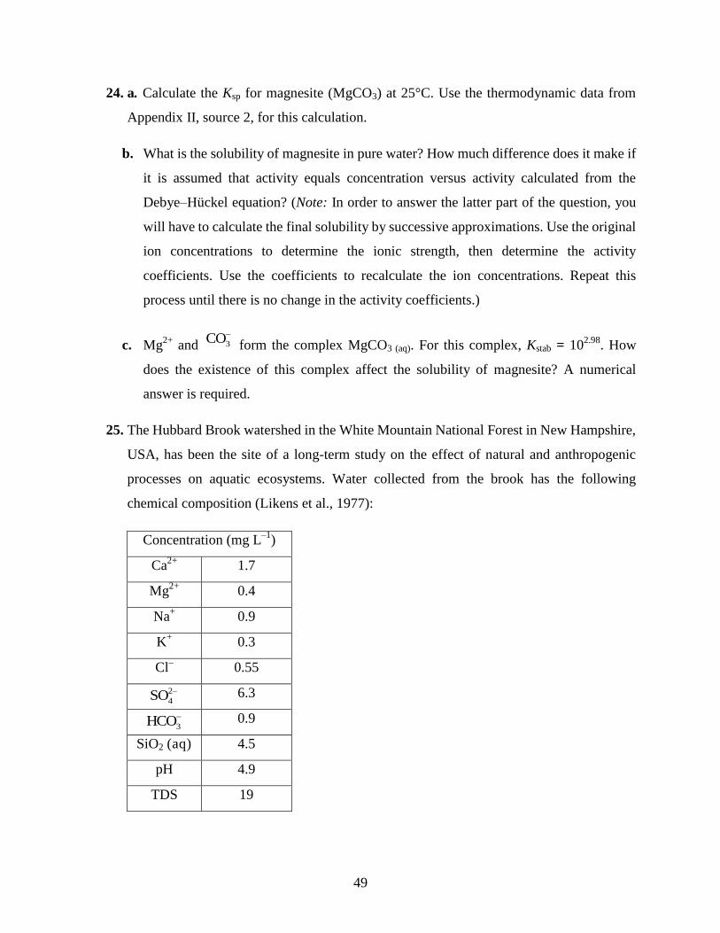
49

24. a. Calculate the Ksp for magnesite (MgCO3) at 25°C. Use the thermodynamic data from

Appendix II, source 2, for this calculation.

b. What is the solubility of magnesite in pure water? How much difference does it make if

it is assumed that activity equals concentration versus activity calculated from the

Debye–Hückel equation? (Note: In order to answer the latter part of the question, you

will have to calculate the final solubility by successive approximations. Use the original

ion concentrations to determine the ionic strength, then determine the activity

coefficients. Use the coefficients to recalculate the ion concentrations. Repeat this

process until there is no change in the activity coefficients.)

c. Mg2+

and 3CO

form the complex MgCO3 (aq). For this complex, Kstab = 102.98

. How

does the existence of this complex affect the solubility of magnesite? A numerical

answer is required.

25. The Hubbard Brook watershed in the White Mountain National Forest in New Hampshire,

USA, has been the site of a long-term study on the effect of natural and anthropogenic

processes on aquatic ecosystems. Water collected from the brook has the following

chemical composition (Likens et al., 1977):

Concentration (mg L–1

)

Ca2+

1.7

Mg2+

0.4

Na+ 0.9

K+ 0.3

Cl– 0.55

2

4SO

6.3

3HCO

0.9

SiO2 (aq) 4.5

pH 4.9

TDS 19

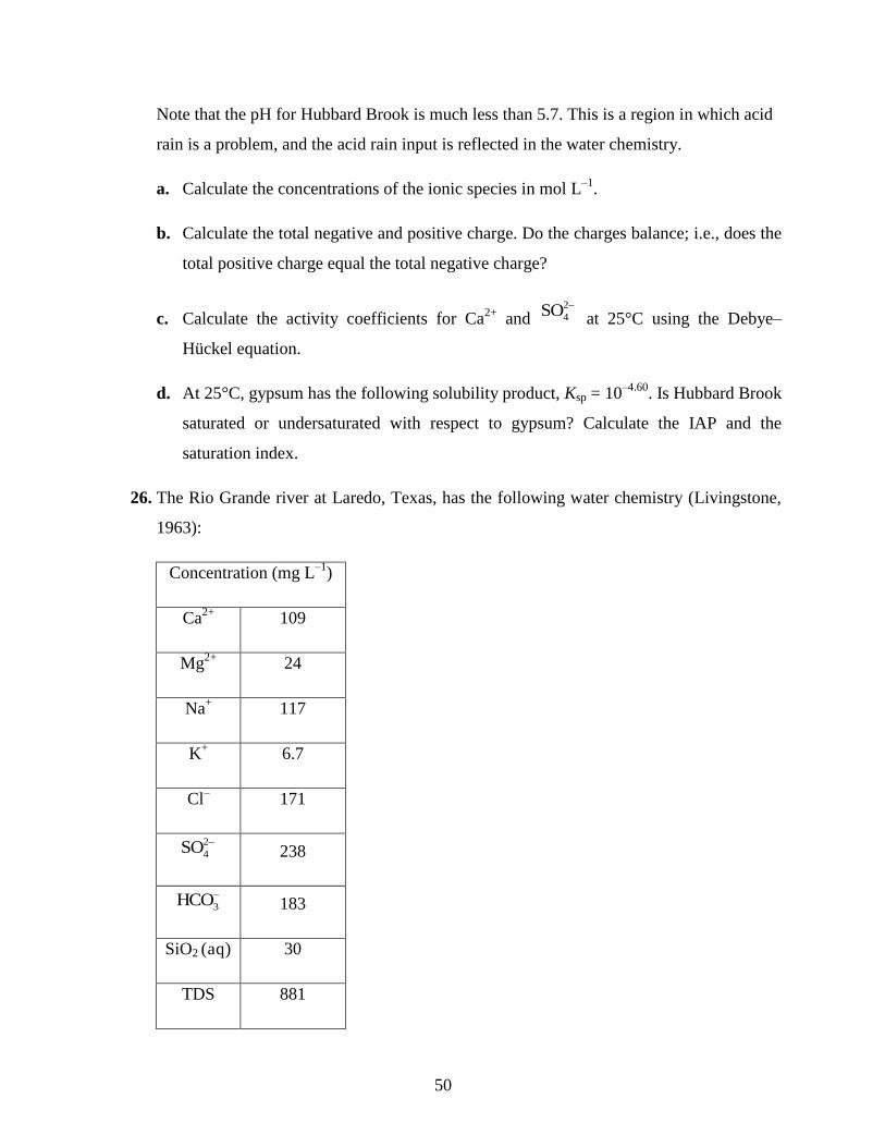
50

Note that the pH for Hubbard Brook is much less than 5.7. This is a region in which acid

rain is a problem, and the acid rain input is reflected in the water chemistry.

a. Calculate the concentrations of the ionic species in mol L–1

.

b. Calculate the total negative and positive charge. Do the charges balance; i.e., does the

total positive charge equal the total negative charge?

c. Calculate the activity coefficients for Ca2+

and 2

4SO

at 25°C using the Debye–

Hückel equation.

d. At 25°C, gypsum has the following solubility product, Ksp = 10–4.60

. Is Hubbard Brook

saturated or undersaturated with respect to gypsum? Calculate the IAP and the

saturation index.

26. The Rio Grande river at Laredo, Texas, has the following water chemistry (Livingstone,

1963):

Concentration (mg L–1

)

Ca2+

109

Mg2+

24

Na+ 117

K+ 6.7

Cl– 171

2

4SO

238

3HCO

183

SiO2 (aq) 30

TDS 881

51

The Rio Grande water chemistry is very different from that of Hubbard Brook (problem

25). Hubbard Brook is located in a forested watershed in the northeastern United States, a

region of temperate climate and moderate rainfall; the Rio Grande is on the U.S.–Mexico

border, a warm region with low annual precipitation. The differences in climate are at least

partly responsible for the differences in water chemistry. Use the thermodynamic data from

Appendix II, source 2, for the following calculations.

a. Calculate the concentrations of the ionic species in mol L–1

b. Calculate the solubility product (equilibrium constant) for gypsum given a water

temperature of 30°C.

c. Calculate the activity coefficient for Ca2+

and 2

4SO

at 30°C using the Debye– Hückel

equation.

d. By how much is the water supersaturated or undersaturated with respect to

CaSO4·2H2O? Your answer should include a numerical estimate.

27. Fluoride is sometimes found in high concentrations in ground and surface waters. Fluoride,

in low concentrations, is often added to drinking water to minimize dental carries, but in

higher concentrations fluoride can pose a health risk. The following table gives the

composition of relatively fluoride-rich waters from three locations: groundwaters drawn

from the Bongo granite, Ghana, groundwaters from Rajasthan, India, and surface waters

from Lake Abiata, Ethiopia. Use the thermodynamic data from Appendix II, source 3, for

the following calculations.

Ground and Surface Water Chemistry (mg L–1

)

Species Bongo granites, Ghana1 Rajasthan, India

2 Lake Abiata, Ethiopia

2

Ca2+

25.3 27.1 1.0

Mg2+

11.5 19.1 0.9

Na+ 23.9 1101 4460

K+ 2.0 5.9 192

Cl– 6.7 617 1911

52

Ground and Surface Water Chemistry (mg L–1

)

Species Bongo granites, Ghana1 Rajasthan, India

2 Lake Abiata, Ethiopia

2

F– 2.3 6.8 119

2

4SO

4.8 500 14.4

3HCO

156 903 8420

1Apambire et al. (1997).

2Apello and Postma (1996).

a. Two minerals that may control the concentration of fluoride ion in solution are fluorite

(CaF2) and villiaumite (NaF). For each of the waters listed in the table, determine the

saturation index at 25°C for these minerals. (Note: Activity is important and must be

included in the calculations.) Would either of these minerals control the fluoride

concentration of these waters?

b. What is a possible explanation for the very high concentrations of Na+, Cl

–, F

–, and

3HCO

in the waters of Lake Abiata? The lake has a pH of 9.62.

28. Knauss et al. (2000) determined various thermodynamic quantities for the aqueous

solubilities of two organic liquids of environmental interest, trichloroethene (TCE) and

tetracholorethene (PCE). The thermodynamic data at 298 K are tabulated here. Note that

the reaction is organic liquid → organic liquid dissolved in water.

∆Gsoln (kJ mol–1

) ∆Hsoln (kJ mol–1

) ∆Ssoln (J mol–1

Κ–1

) ∆Cp soln (J mol–1

Κ–1

)

TCE 11.282 –3.35 –49.07 385.2

PCE 15.80 –1.79 –59.00 354.6

a. Calculate the equilibrium constants for both reactions.

b. If 1 kg of each organic liquid was spilled into 1000 kg of water, calculate the

concentration of each organic liquid dissolved in the water.

53

c. Using Le Châtelier’s principle, predict what would happen to the solubility of each

organic liquid in water with increasing temperature.

d. For each organic liquid calculate the equilibrium constant at 40°C. Were the predictions

you made using Le Châtelier’s principle, part (c), correct?

29. Asbestos minerals are considered to be a health hazard. The most common type of asbestos

is chrysotile, and this mineral comprises about 95% of the asbestos in the United States.

Small asbestos fibers can be taken into the lung, where they interact with the lining of the

lung. This problem deals with the solubility of chrysotile asbestos in the lung. A later

problem deals with the rate at which chrysotile fibers will break down in the lung. The

dissolution reaction for chrysotile can be written

Mg3Si2O5(OH)4 chrysotile + 6H+ → 3Mg

2+ + 2H4SiO4(aq) + H2O

Use the thermodynamic data from Appendix II, source 3, for the following calculations.

a. Calculate the equilibrium constant for this reaction at T = 37°C, the average

temperature of the human body.

b. For fluid in lung tissues, pH = 4, Mg2+

= 8.7 × 10–4

mol L–1

, and H4SiO4(aq) = 1.5 × 10–

6 mol L

–1. Assume activity equals concentration. Are the lung fluids under– or

oversaturated with respect to chrysotile? Give a numerical answer.

c. Redo the calculation in part (b) given an ionic strength for the lung fluids of 0.12.

d. Based on these calculations, would you expect chrysotile to persist in the lungs?

Explain your answer.

30. Knauss et al. (2000) determined Henry’s law constants for TCE and PCE at various

temperatures. Henry’s law is often expressed as

Concentration vapor

Concentration liquidcH

which is the form of Henry’s law used by Knauss et al. (2000).

54

TCE PCE

T (K) Hc (atm m3 mol

–1 ) T (K) Hc (atm m

3 mol

–1)

294 0.006942 295 0.017574

323 0.025183 324 0.057607

348 0.048869 348 0.121925

372 0.067645 374 0.182980

390 0.060473 397 0.189062

a. 1 × 10–4

mol m–3

of TCE are dissolved in water at 294 K. Calculate the equilibrium

vapor pressure.

b. 1 × 10–5

mol m–3

of PCE are dissolved in water at 324 K. Calculate the equilibrium

vapor pressure.

31. At 25°C and pH = 5, the following dissolution rates have been obtained for quartz,

microcline, albite, diopside, forsterite, and anorthite (data from Lasaga et al., 1994). These

dissolution reactions are zeroth-order reactions.

Mineral Formula Density g

cm–3

Log rate mol

m–2

s–1

Quartz SiO2 2.65 –13.39

Microcline KAlSi3O8 2.59 –12.50

Albite NaAlSi3O8 2.62 –12.26

Diopside CaMgSi2O6 3.22 –10.15

Forsterite Mg2SiO4 3.22 –9.50

Anorthite CaAl2Si2O8 2.76 –8.55

Assuming a planar surface, calculate how long it will take to dissolve a 1-mm-thick layer

from each of the minerals. Note that the dissolution rates are determined for a square

meter of surface area, so you should do these calculations for 1 m2 of surface area

55

retreating 1 mm. You will first need to calculate the total moles of each mineral in the

volume to be removed. Then calculate the dissolution times, in years, for each mineral.

Compare these dissolutions times to the preservation/loss of these minerals during

weathering and transport. Is there a relationship between the dissolution times and the

persistence of these minerals in the weathering environment?

32. Hume and Rimstidt (1992) investigated the dissolution of chrysotile in lung solutions.

They found that the rate-controlling step is the release of Si to solution, and that the

reaction is zeroth order. The experimentally determined rate constant is k = 5.9 × 10–10

mol

m–2

s–1

. They modeled the breakdown of a fiber as if it were an infinitely long cylinder

dissolving over its lateral surface. The resulting equation is

3

/4

mt d V k

where t is the time in seconds, d is the diameter of the fiber in meters, Vm is the volume

occupied by 1 mol of silica in chrysotile (5.4 × 10–5

m3 mol

–1), and k is the rate constant.

Calculate the dissolution time for a chrysotile fiber 1 μm in diameter.

33. Foos (1997) determined a first-order rate constant for the removal of Fe2+

from a stream

(Case Study 2–1). Discharge from a point source adds Fe2+

to a river. Using the rate

constant determined by Foos (1997) and a stream velocity of 0.5 m s–1

, calculate the

transport distance required to achieve a 90% reduction in the amount of Fe2+

in solution. To

do this problem you will first need to find the amount of time required to reduce the iron

concentration by 90%.

34. The breakdown of pyrite (and marcasite) is important in determining the pH of waters

draining from coal mines and spoils (acid mine drainage). Aqueous oxidation of pyrite by

molecular oxygen can be represented by the following reaction:

2 2

2pyrite 2 2 4

7FeS O H O Fe 2SO 2H

2

For this reaction, Williamson and Rimstidt (1994) determined the following rate constant:

56

0.58.19 DO

0.11

H

10m

rm

where mDO is the amount of dissolved oxygen, Hm is the hydrogen ion concentration,

and r is the rate of pyrite destruction in mol m–2

s–1

. Assume the activation energy for this

reaction is 60 kJ mol–1

. Spoils from a coal mine contain small pyrite cubes having an

average specific surface area of 0.01 m2 g

–1. Water percolating down through this spoils

pile is saturated with respect to atmospheric oxygen (10–3.6

mol L–1

). The water has a pH

of 5.0. Assume that the breakdown of pyrite only occurs according to the preceding

reaction.

a. Calculate the rate constant for the breakdown of pyrite in contact with the water

percolating through the spoils pile.

b. Given that the reaction is pseudo zero order, calculate the time required (t1/2) for

oxidation of half the pyrite in the spoils pile. You will first need to calculate the

number of moles in 1 g of pyrite, and then determine the moles per square meter of

specific surface area. The result of this calculation is the value for A0 in the rate

equation.

c. If the reaction rate was determined at 20°C, calculate the reaction rate at 30°C.

35. Several studies have been done on the rate at which organic matter breaks down in the

marine environment. Westerich and Berner (1984) identified three types of organic matter

in marine sediments—highly reactive, less reactive, and nonreactive (didn’t break down

during the course of their experiments). The following equation summarizes the results of

their experiments:

GT(t) = G01[exp(–k1t)] + G02[exp(–k2t)] + Gnr

where GT is the total organic carbon, G01 is the highly reactive fraction, G02 is the less

reactive fraction, and Gnr is the nonreactive fraction. Different rate constants were

determined for oxic and anoxic decay. Middelburg (1989) developed a different model that

expressed the decay of organic matter in marine sediments in terms of a single first-order

57

rate equation in which k changes with time. The following equation relates the rate constant

and its change with time:

log k = –0.95 log t – 0.81

and

Gt1 = Gt0 exp 3.2(–t0.05

)

where Gt1 is the amount of organic carbon remaining at time t, Gt0 is the amount of organic

carbon initially present, and t is time.

For a number of years New York City has disposed of its sewage sludge in the New

York Bight.

a. Using the model of Westerich and Berner (1984), calculate the amount of sludge

remaining 1 year after deposition in the New York Bight. Assume that the sewage

consists of 45% highly reactive organic carbon, 45% less reactive organic carbon, and

10% nonreactive organic carbon. For oxic decay, k1 = 18 y–1

and k2 = 2.3 y–1

.

b. Do the same calculation as in (a) using the model of Middelburg (1989).

c. Compare the two answers. Why are they different?

d. Using the equation of Middelburg (1989), calculate the length of time it will take for

50% and 99% of the organic matter to decompose. Are both of these answers realistic?

You may want to read the original paper to get a better understanding of the model.

36. The dissolution of quartz in H2O can be represented by the following reaction:

SiO2 (s) + 2H2O → H4SiO4 (aq)

Rimstidt and Barnes (1980) determined the reaction rate for the dissolution of quartz as a

function of temperature. Their data are listed in the following table:

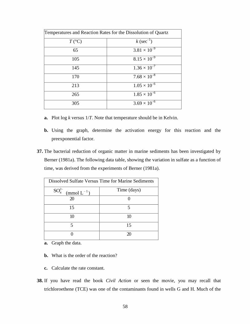
58

Temperatures and Reaction Rates for the Dissolution of Quartz

T (°C) k (sec–1

)

65 3.81 × 10–9

105 8.15 × 10–9

145 1.36 × 10–7

170 7.68 × 10–8

213 1.05 × 10–6

265 1.85 × 10–6

305 3.69 × 10–6

a. Plot log k versus 1/T. Note that temperature should be in Kelvin.

b. Using the graph, determine the activation energy for this reaction and the

preexponential factor.

37. The bacterial reduction of organic matter in marine sediments has been investigated by

Berner (1981a). The following data table, showing the variation in sulfate as a function of

time, was derived from the experiments of Berner (1981a).

Dissolved Sulfate Versus Time for Marine Sediments

2

4SO

(mmol L– 1

) Time (days)

20 0

15 5

10 10

5 15

0 20

a. Graph the data.

b. What is the order of the reaction?

c. Calculate the rate constant.

38. If you have read the book Civil Action or seen the movie, you may recall that

trichloroethene (TCE) was one of the contaminants found in wells G and H. Much of the

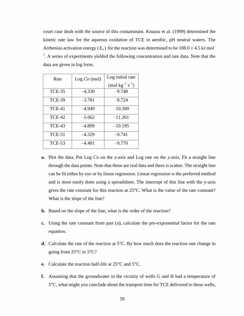
59

court case dealt with the source of this contaminant. Knauss et al. (1999) determined the

kinetic rate law for the aqueous oxidation of TCE in aerobic, pH neutral waters. The

Arrhenius activation energy ( Ea ) for the reaction was determined to be 108.0 ± 4.5 kJ mol–

1. A series of experiments yielded the following concentration and rate data. Note that the

data are given in log form.

Run Log Co (mol) Log initial rate

(mol kg–1

s–1

)

TCE-35 –4.330 –9.748

TCE-39 –3.781 –9.724

TCE-41 –4.949 –10.300

TCE-42 –5.662 –11.261

TCE-43 –4.899 –10.195

TCE-51 –4.329 –9.741

TCE-53 –4.401 –9.770

a. Plot the data. Put Log Co on the x-axis and Log rate on the y-axis. Fit a straight line

through the data points. Note that these are real data and there is scatter. The straight line

can be fit either by eye or by linear regression. Linear regression is the preferred method

and is most easily done using a spreadsheet. The intercept of this line with the y-axis

gives the rate constant for this reaction at 25°C. What is the value of the rate constant?

What is the slope of the line?

b. Based on the slope of the line, what is the order of the reaction?

c. Using the rate constant from part (a), calculate the pre-exponential factor for the rate

equation.

d. Calculate the rate of the reaction at 5°C. By how much does the reaction rate change in

going from 25°C to 5°C?

e. Calculate the reaction half-life at 25°C and 5°C.

f. Assuming that the groundwater in the vicinity of wells G and H had a temperature of

5°C, what might you conclude about the transport time for TCE delivered to these wells,

60

i.e., would it be months or years? Explain your answer. In answering this question you

need to consider how long TCE would persist in the groundwater under these

conditions. If it has already degraded by the time the water reaches the well, it wouldn’t

be found in the well water.