1

PROBABILITY MODELS FOR ECONOMIC DECISIONS

Chapter 2: Discrete Random Variables

In this chapter, we focus on one simple example, but in the context of this example we

develop most of the technical concepts of probability theory, statistical inference, and decision

analysis that be used throughout the rest of the book. This example is very simple in that it

involves only one unknown quantity which has only finitely many possible values. That is, in

technical terms, this example involves just one discrete random variable.

With just one discrete random variable, we can make a table or chart that completely

describes its probability distribution. Among the various ways of picturing a probability

distribution, the most useful in this book will be the inverse cumulative distribution chart. After

introducing such charts and explaining how to read them, we show how this inverse cumulative

distribution can be used to make a simulation model of any random variable.

Next in this chapter we introduce the two most important summary measures of a random

variable's probability distribution: its expected value and standard deviation. These two

summary measures can be easily computed for a discrete random variable, but we also show how

to estimate these summary measures from simulation data. The expected value of a decision-

maker's payoff will have particular importance throughout this book as a criterion for identifying

optimal decisions under uncertainty.

Later in the book we will consider more complex models with many random variables,

some of which may have infinitely many possible values. For such complex models, we may not

know how to compute expected values and standard deviations directly, but we will still be able

to estimate these quantities from simulation data by the methods that are introduced in this

chapter. We introduce these methods here with a simple one-variable model because, when you

first learn to compute statistical estimates from simulation data, it is instructive to begin with a

case where you can compare these estimates to the actual quantities being estimated.

2

Case: SUPERIOR SEMICONDUCTOR (Part A)

Peter Suttcliff, an executive vice-president at Superior Semiconductor, suspected that the

time might be right for his firm to introduce the first integrated T-regulator device using new

solid-state technology. This new product seemed the most promising of the several ideas that

had been suggested by the head of Superior's Industrial Products division. So Suttcliff asked his

staff assistant Julia Eastmann to work with Superior's business marketing director and the chief

production engineer to develop an evaluation of the profit potential from this new product.

According to Eastmann's report, the chief engineer anticipated substantial fixed costs for

engineering and equipment just to set up a production line for the new product. Once the

production line was set up, however, a low variable cost per unit of output could be anticipated,

regardless of whether the volume of output was low or high. Taking account of alternative

technologies available to the potential customers, the marketing director expressed a clear sense

of the likely selling price of the new product and the potential overall size of the market. But

Superior had to anticipate that some of its competitors might respond in this area by launching

similar products. To be specific in her report, Eastmann assumed that 3 other competitive firms

would launch similar products, in which case Superior should expect 1/4 of the overall market.

Writing in the margins of Eastmann's report, Suttcliff summarized her analysis as

follows:

C Superior's fixed set-up cost to enter the market: $26 million

C Net present value of revenue minus variable costs in the whole market: $100 million

C Superior's predicted market share, assuming 3 other firms enter: 1/4

C Result: predicted net loss for Superior: ($1 million)

"Your estimates of costs and total market revenues look reasonably accurate," Suttcliff

told Eastmann. "But your assumption about the number of other firms entering to share this

market with us is just a guess. I can count 5 other semiconductor firms that might seriously

consider competing with us in this market. In the worst possible scenario, all 5 of these firms

could enter the market, although that is rather unlikely. There is no way that we could keep this

market to ourselves for any length of time, and so the best possible scenario is that only 1 other

firm would enter the market, although that is also rather unlikely. I would agree with you that the

most likely single event is that 3 other firms would enter to share the market with us, but that

event is only a bit more likely than the possibilities of having 2 other firms enter, or having 4

other firms enter. If there were only 2 other entrants, it could change a net loss to a net profit. So

there is really a lot of uncertainty about this situation, and your analysis might be more

convincing if you did not ignore it."

"We can redo the analysis in a way that takes account of the uncertainty by using a

3

probabilistic model," Eastmann replied. "The critical step is to assess a probability distribution

for the unknown number of competitors who would enter this market with us. So I should try to

come up with a probability distribution that summarizes the beliefs that you expressed." Then

after some thought, she wrote the following table and showed it to Suttcliff:

K Probability that K other competitors enter

1 0.10

2 0.25

3 0.30

4 0.25

5 0.10

Suttcliff studied the table. "I guess that looks like what I was trying to say. I can see that

your probabilities sum to 1, and you have assigned higher probabilities to the events that I said

were more likely. But without any statistical data, is there any way to test whether these are

really the right probability numbers to use?"

"In a situation like this, without data, we have to use subjective probabilities," Eastmann

explained. "That means that we can only go to our best expert and ask him whether he believes

each possible event to be as likely as our probabilities say. In this case, if we take you as best

expert about the number of competitive entrants, then I could test this probability distribution by

asking you questions about your preferences among some simple bets. For example, I could ask

you which you would prefer among two hypothetical lotteries, where the first lottery would pay

you a $10,000 prize if exactly one other firm entered this market, while the second lottery would

pay the same $10,000 prize but with an objective 10% probability. Assuming that you had no

further involvement with this project, you should be indifferent among these two hypothetical

lotteries if your subjective probability of one other firm entering is 0.10, as my table says. If you

said that you were not indifferent, then we would try increasing or decreasing the first probability

in the table, depending on whether you said that the first or second lottery was preferable. Then

we could test the other probabilities in the table by similar questions. But if we change any one

probability in my table then at least one other probability must be changed, because the

probabilities of all the possible values of the unknown quantity must add up to 1."

Suttcliff looked again at the table of probabilities for another minute or two, and then he

indicated that it seemed to be a reasonable summary of his beliefs.

4

2.1 Unknown quantities in decisions under uncertainty

Uncertainty about numbers is pervasive in all management decisions. How many units of

a proposed new product will we sell in the year when it is introduced? How many yen will a

dollar buy in currency markets a month from today? What will be the closing Dow Jones

Industrial Average on the last trading day of this calendar year? Each of these number is an

unknown quantity. If our profit or payoff from a proposed strategy depends on such unknown

quantities, then we cannot compute this payoff without making some prediction of these

unknown quantities.

A common approach to such problems is to assess your best estimate for each of these

unknown quantities, and use these estimates to compute the bottom-line payoff for each proposed

strategy. Under this method of point-estimates, the optimal strategy is considered to be the one

that gives you the highest payoff when all unknown quantities are equal to your best estimates.

But there is a serious problem with this method of point-estimates: It completely ignores

your uncertainty. In this book, we study ways to incorporate uncertainty into the analysis of

decisions. Our basic method will be to assess probability distributions for unknown quantities,

and then to create random variables that simulate these unknown quantities in spreadsheet

simulation models.

In the general terminology of decision analysis, the term "random variable" is often taken

by definition to mean the same thing as the phrase "unknown quantity." But as a matter of style

here, we will generally reserve the term unknown quantity for unknowns in the real world, and

random variable will be generally used for values in spreadsheets that are unknown because they

depend on unknown RAND values.

To illustrate these ideas, we consider the Superior Semiconductor case (Part A). In this

case, we have a decision about whether our company should introduce a proposed new product.

It is estimated that the fixed cost of introducing this new product will be $26 million. The total

value of the market (price minus variable unit costs, multiplied by total demand) is estimated to

be $100 million. It is also estimated that 3 other firms will enter this market and share it equally

with us. Thus, by the method of point-estimates, we get a net profit (in $millions) of

100'(3+1)!26 = !1, which suggests that this product should not be introduced. But all the

5

quantities in this calculation (fixed cost, value of the market, number of competitive entrants) are

really subject to some uncertainty. We will see, however, that when uncertainty is properly taken

into account, the new product may be recognized as worth introducing.

The analysis in Part A of this case focuses on just one of these unknowns: the number of

entrants. Uncertainty about other quantities (fixed cost, value of the market) is ignored until the

end of this chapter, but it will be considered in more detail in Chapter 4. By focusing on just this

one unknown quantity for now, we can simplify the analysis as we introduce some of the most

important fundamental ideas of probability theory.

2.2 Charting a probability distribution

We use probability distributions to describe people's beliefs about unknown quantities.

When an unknown quantity has only finitely many possible values, we can describe it using a

discrete probability distribution. (Continuous probability distributions, for unknown quantities

with infinitely many possible values, will be discussed in Chapter 4.) A discrete probability

distribution can be presented in a table that lists the possible values of the unknown quantity and

the probability of each possible value.

In the Superior Semiconductor case, the number of competitors who will enter the market

is a quantity that is unknown to the company's decision-makers, and they believe that this

unknown quantity could be any number from 1 to 5. In our mathematical notation, let K denote

this unknown number of competitors who will enter this market. (I follow a mathematical

tradition of representing unknown quantities by boldface letters.) Then the decision-maker's

beliefs about this unknown quantity K are described in the case by a discrete probability

distribution such that

P(K=1) = 0.10, P(K=2) = 0.25, P(K=3) = 0.30, P(K=4) = 0.25, P(K=5) = 0.10 .

Here for any number k, the mathematical expression P(K=k) denotes the probability that the

unknown quantity K is equal to the value k. This probability distribution summarized by a chart

in Figure 2.1.

0.0

0.1

0.2

0.3

0.4

0.5

0.6

0.7

0.8

0.9

1.0

0 1 2 3 4 5 6Number of competitive entrants (K)

Pro

babi

lity

Dashed lines: Cumulative Probability

6

Figure 2.1. Discrete Probability Distribution for the Number of Entrants (K).

Figure 2.1 actually displays this probability distribution in two different ways. The five

solid bars in Figure 2,1 show the probabilities of the five points on the horizontal axis that

represent possible values of the unknown quantity K. Such point-probability bars are the most

common way of exhibiting a discrete probability distribution. But Figure 2.1 also contains a

dashed line that shows cumulative probability values, which we must now explain.

A cumulative probability of the unknown quantity K at a number k is the probability of K

being below the value k. It is a question of mathematical convention as to whether "cumulative

probability of K at 2" should be precisely defined as P(K<2) or P(K#2), that is, 0.10 or

0.10+0.25 = 0.35 in this case. In most books the latter definition is used. But in this book, let us

eclectically embrace both definitions and everything in between, and define a cumulative

probabilities of K at k to include P(K<k) and P(K#k) and every number in between. So in this

terminology, any number between 0.10 and 0.35 can be called a cumulative probability of K at 2

in this example. But notice that such ambiguity only occurs at numbers that have positive

7

probability for the random variable. For example, the cumulative probability of K at 2.5 is 0.35,

because P(K<2.5) = P(K#2.5) = 0.10 + 0.25 = 0.35.

The dashed curve in Figure 2.1 as representing shows the cumulative probabilities for

each number k on the horizontal axis. For any number k between 1 and 2, the height of the

dashed cumulative-probability curve in Figure 2.1 is 0.10, because P(K<k) = P(K#k) = P(K=1) =

0.10 when 1<k<2. For any number k between 2 and 3, the height of the dashed cumulative-

probability curve in Figure 2.1 is 0.35, because

P(K<k) = P(K#k) = P(K=1) + P(K=2) = 0.10 + 0.25 = 0.35 when 2<k<3.

The unknown quantity K is sure to be less than 6, and so the height of the cumulative

probability-curve at 6 is 1 = P(K<6). The unknown quantity K is sure to not be less than 0, and

so the height of the cumulative-probability curve at 0 is 0 = P(K<0).

In Figure 2.1, the dashed cumulative-probability curve has vertical jumps (representing

multiple cumulative probabilities from P(K<k) to P(K#k)) exactly where the point-probability

bars occur, and the height of each vertical jump is the same as the height of the corresponding

point-probability bar. For example, the dashed cumulative-probability curve jumps from 0.10 to

0.35 above the value 2 on the horizontal axis of Figure 2.1, which corresponds to the fact that

P(K=2) = 0.25 = 0.35!0.10. So the cumulative-probability curve tells us everything about the

probability distribution that we could learn from the point-probability bars. This observation is

important, because we will find that cumulative-probability curves are generally more useful for

describing probability distributions than point-probability bars (which cannot be applied to

continuous probability distributions where there are infinitely many possible values).

Actually, we will find it most useful to invert the cumulative probability distribution,

turning the dashed line from Figure 2.1 on its side, with cumulative probabilities on the

horizontal axis and possible values of K on the vertical axis. Such an inverse cumulative-

probability curve is shown in Figure 2.2. Once you learn how to read it, you can find the discrete

probabilities of all possible values of K from this inverse cumulative-probability curve. For

example, the inverse cumulative-probability curve has height 2 over the interval of probabilities

from 0.10 to 0.35, which tells us that the point-probability of the value 2 is P(K=2) = 0.35!0.10

= 0.25. The height of the inverse cumulative-probability curve goes from 1 to 5 because these

0

1

2

3

4

5

6

0.0 0.1 0.2 0.3 0.4 0.5 0.6 0.7 0.8 0.9 1.0

Cumulative Probability

Num

ber

ofco

mpe

titiv

een

tran

ts(K

)

8

Figure 2.2. Inverse cumulative probability curve for number of entrants (K).

are the lowest and highest possible values of the unknown K. (Because we will generally draw

our cumulative charts in this inverse orientation, it should also be acceptable here to drop the

word "inverse" and simply refer to a chart like Figure 2.2 as a "cumulative probability" chart.)

For any numbers q and k, if q is a cumulative probability of an unknown quantity K at the

k, then we may also say that k is a q-percentile value of K. So in this example, the 0.2-percentile

value of K is 2, but any number from 2 to 3 could be called a 0.35-percentile value of K.

2.3 Simulating discrete random variables

When we say that a random variable in a spreadsheet simulates (or represents) some

unknown quantity in real life, we mean that any event for this simulated random variable is, from

the perspective of our current information and beliefs, just as likely as the same event for the real

unknown quantity. If the unknown number of competitive entrants has a probability 0.10 of

equaling 1, for example, then the random variable in the spreadsheet should also have probability

9

0.10 of equaling 1 after the next recalculation of the spreadsheet. For any number k, the

probability that the random variable will be less than k after the next recalculation should be the

same as the probability that the real unknown quantity is less than k.

In our spreadsheets, all our random variables are constructed as functions of RAND()

values. So recall how the RAND function operates: Given any two numbers x and y such that

0 # x # y # 1, the event that some particular RAND() in a spreadsheet formula will take a value

between x and y after the next recalculation is equal to the difference y!x, that is,

P(x # RAND() # y) = y ! x.

For example, the probability that a RAND() will be between 0 and 0.10 is 0.10, and the

probability that the RAND() will be between 0.10 and 0.35 is 0.35!0.10 = 0.25.

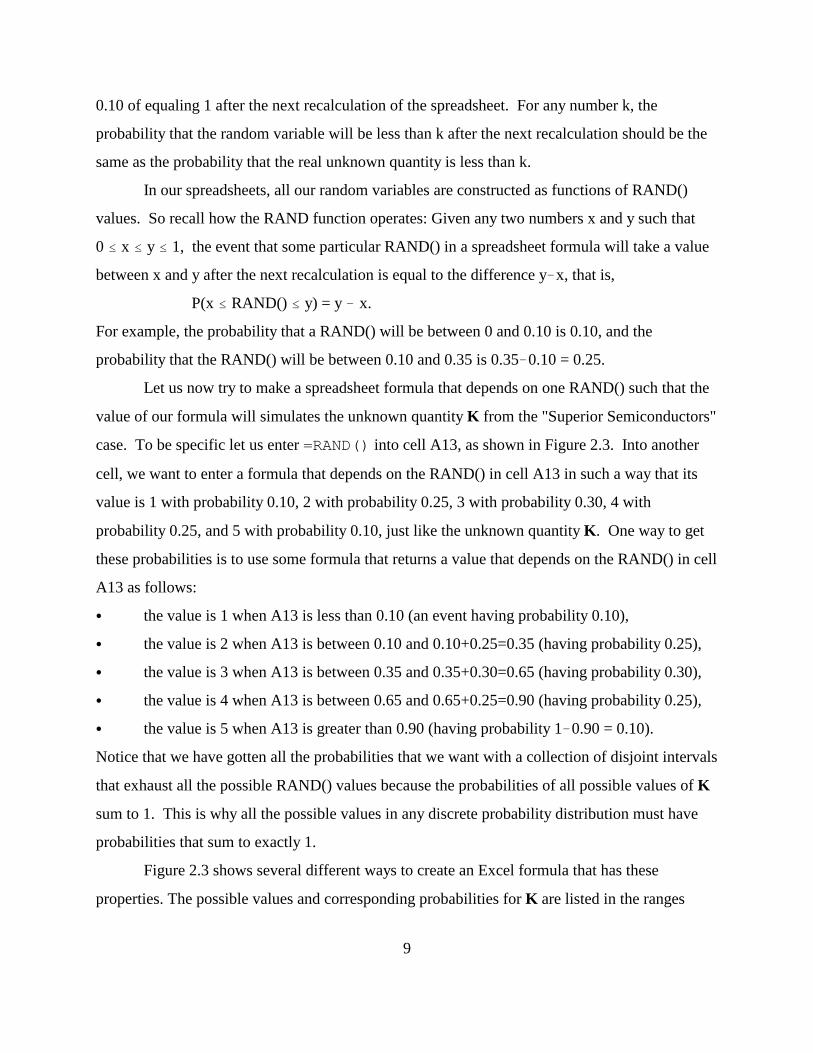
Let us now try to make a spreadsheet formula that depends on one RAND() such that the

value of our formula will simulates the unknown quantity K from the "Superior Semiconductors"

case. To be specific let us enter =RAND() into cell A13, as shown in Figure 2.3. Into another

cell, we want to enter a formula that depends on the RAND() in cell A13 in such a way that its

value is 1 with probability 0.10, 2 with probability 0.25, 3 with probability 0.30, 4 with

probability 0.25, and 5 with probability 0.10, just like the unknown quantity K. One way to get

these probabilities is to use some formula that returns a value that depends on the RAND() in cell

A13 as follows:

C the value is 1 when A13 is less than 0.10 (an event having probability 0.10),

C the value is 2 when A13 is between 0.10 and 0.10+0.25=0.35 (having probability 0.25),

C the value is 3 when A13 is between 0.35 and 0.35+0.30=0.65 (having probability 0.30),

C the value is 4 when A13 is between 0.65 and 0.65+0.25=0.90 (having probability 0.25),

C the value is 5 when A13 is greater than 0.90 (having probability 1!0.90 = 0.10).

Notice that we have gotten all the probabilities that we want with a collection of disjoint intervals

that exhaust all the possible RAND() values because the probabilities of all possible values of K

sum to 1. This is why all the possible values in any discrete probability distribution must have

probabilities that sum to exactly 1.

Figure 2.3 shows several different ways to create an Excel formula that has these

properties. The possible values and corresponding probabilities for K are listed in the ranges

10

B5:B9 and C5:C9 of Figure 2.3. The (low) cumulative probabilites of the various possible

values are computed from this probability distribution in cells A5:A9 of Figure 2.3. Cell G5

contains the formula

=IF($A$13<A6,B5,0)

So cell G5 equals 1 (B5) if the RAND in A13 satisfies the inquality A13 < A6 = 0.10, and

G5 equals 0 otherwise. Cell G6 contains the formula

=IF(AND(A6<=$A$13,$A$13<A7),B6,0)

Excel's AND function returns the logical value TRUE if all of its parameters are TRUE, and

otherwise AND returns the logical value FALSE. So by the IF function in this formula, cell G6

equals 2 (B6) when the RAND in A13 is satisfies the inequalities 0.10 = A6 # A13 < A7 = 0.35,

and G6 equals 0 otherwise. (Excel uses <= to denote less-than-or-equal-to, and uses >= to

denote greater-than-or-equal-to.) The other formulas in cells G5:G9 are constructed similarly so

that one of these cells will equal the possible value of K that would be designated by the

RAND() in cell A13 under the above rule, while all the other cells in G5:G9 will equal 0. Thus,

the formula =SUM(G5:G9) in cell B13 returns the random variable that we wanted.

Simtools provides a function called DISCRINV to accomplish this same calculation

more easily. As you can verify by consulting the Insert-Function dialogue box, the DISCRINV

function takes three parameters. The first parameter (which is called "randprob" in the Insert-

Function dialogue box) should simply be a RAND(). The second parameter (called "values")

should be a range that lists the possible values of our discrete random variable. The third

parameter (called "probabilities"), should be another range which has the same size as the values

range and which lists the corresponding probabilities of these values. Then the formula

DISCRINV(RAND(), values, probabilities)

returns a random variable that has values and discrete probabilities as listed in these ranges. In

this spreadsheet, the formula =DISCRINV(A13,B5:B9,C5:C9) in cell B14 returns a random

variable that depends on the RAND in A13 according to the rule that we described above, and so

the value of cell B14 is always the same as cell B13 for any value of the RAND in cell A13.

The cell B15 contains a rather ugly formula that does the job in one line

=IF(A13<A6,B5,IF(A13<A7,B6,IF(A13<A8,B7,IF(A13<A9,B8,B9))))

1234567891011121314151617181920212223242526272829

A B C D E F G HA DISCRETE RANDOM VARIABLE FROM THE "SUPERIOR SEMICONDUCTOR" CASE

K = (unknown number of competitors entering market).Little k = (possible value of big K).

P(K<k) k P(K=k) (for B16)0.00 1 0.10 00.10 2 0.25 20.35 3 0.30 00.65 4 0.25 00.90 5 0.10 0

1

Simulated value0.32748 2

222

FORMULASA6. =A5+C5A6 copied to A6:A9

C10. =SUM(C5:C9)A13. =RAND()G5. =IF($A$13<A6,B5,0)G6. =IF(AND(A6<=$A$13,$A$13<A7),B6,0)G6 copied to G6:G8

G9. =IF(A9<=$A$13,B9,0)B13. =SUM(G5:G9)B14. =DISCRINV(A13,B5:B9,C5:C9)B15. =IF(A13<A6,B5,IF(A13<A7,B6,IF(A13<A8,B7,IF(A13<A9,B8,B9))))B16. =VLOOKUP(A13,A5:B9,2)

11

Figure 2.3. Simulation with a discrete probability distribution (4 equivalent formulas).

I do not recommend using this formula. First, when a formula is so complicated, your chances of

typing it incorrectly are very high. Second, this method cannot be applied to larger problems,

because Excel may refuse to consider formulas where functions that are nested more than 8

parentheses deep. Cell B16 illustrates another more elegant way to compute the same random

variable using the Excel function VLOOKUP.

At this point you may wonder why the Simtools function for simulating a discrete random

variable should be called DISCRINV. The letters "DISC" obviously come from the word

"discrete," But what does the "INV" signify? To see the answer, notice that this function has

been designed to return the value 1, 2, 3, 4, or 5, depending on the value of the RAND() that is its

12

first parameter, and the points where the function's value changes are 0.10, 0.10+0.25 = 0.35,

0.35+0.30 = 0.65, and 0.65+0.25 = 0.90. You have seen a function like this before: It is the

inverse cumulative function shown in Figure 2.2. Indeed, the "INV" in our function's name is

short for "inverse cumulative."

In general, any random variable can be simulated by processing a RAND() through the

inverse cumulative-probability function. If a function G(C) is the inverse cumulative-probability

function of an unknown quantity X then, for any numbers k and q, we get G(q) < k when

q < P(X<k). So for any number k, the random variable G(RAND()) will be less than k when the

RAND() is in the interval from 0 to P(X<k), which occurs with probability P(X<k). So

G(RAND()) has the same probability distribution as X.

The bottom-line quantity of interest in the Superior Semiconductor case is profit. If we

assume that the $100 million total value of the market will be shared equally by Superior

Semiconductor and its K competitors then, after deducting $26 million of fixed costs, then

Superior Semiconductor's profit (in $millions) should depend on the number of competitors K by

the formula

Profit = 100'(1+K) ! 26

So if K equals 1 then profit is 100'(1+1)!26 = 24 ($million), but if K equals 5 then profit is

100'(1+5)!26 = !9.33. So profit is also an unknown quantity, with a discrete probability

distribution as shown in the following table:

Competitors Profit Probability

1 24 0.10

2 7.33 0.25

3 !1 0.30

4 !6 0.25

5 !9.33 0.10

Figure 2.4 shows two attempts to make a model in which the number of competitors and the

resulting profit for Superior Semiconductors are both simulated.

123456789101112131415161718192021222324252627

A B C D E F G"SUPERIOR SEMICONDUCTOR" CASE 26 FixedCost

100 MarketValueLet K = (unknown number of competitors entering market)

k P(K=k) Profit (in $millions)1 0.10 24.002 0.25 7.333 0.30 -1.004 0.25 -6.005 0.10 -9.33

1 sum

Model 1 (correct)#Competitors entering Profit

2 7.33

Model 2 (WRONG!!!)#Competitors entering Profit

4 24

FORMULAS FROM RANGE A1:F18E5. =$E$2/(1+B5)-$E$1E5 copied to E5:E9

C10. =SUM(C5:C9)B14. =DISCRINV(RAND(),B5:B9,$C$5:$C$9)E14. =$E$2/(1+B14)-$E$1B18. =DISCRINV(RAND(),B5:B9,$C$5:$C$9)E18. =DISCRINV(RAND(),E5:E9,$C$5:$C$9)

13

Figure 2.4. Making a simple simulation model of competitors and profit.

The range B16:E18 in Figure 2.4 contains an attempt, called "Model 2," which illustrates

one of the most common errors that students make in simulation modeling. In Model 2, the

number of competitors and the profit are simulated in cells B18 and E18 respectively, with two

DISCRINV formulas that depend on separate RANDs. The result is that profit is independent of

the number of competitors in Model 2, which is wrong. For example, Figure 2.4 shows a

realization of these random variables such that the simulated number of competitors in B18 is 4

while the simulated profit in E18 is 24 ($million); but if there were really 4 competitive entrants

then Superior Semiconductor's profit would be 100'(1+4)!26 = !6.

The range B12:E14 in Figure 2.4 contains "Model 1," which is done correctly. In this

14

model, the number of competitors is simulated by a DISCRINV formula in cell B14, while the

profit is simulated in cell E14 as a function of the simulated number of competitors by the

formula =$E$2'(1+B14)!$E$1 (where E2 contains the market value 100 and E1 contains

the fixed cost 26). Thus Model 1 always displays the correct relationship between the number of

competitors and the profit.

In general, a simulation model is a good representation of a real situation if our

uncertainty about the next recalculated values of the random variables in the model (that is, what

they will be after we next press [F9]) is the same as our uncertainty about the corresponding

unknown quantities in the real situation. Fancy formulas in a spreadsheet obviously cannot be

asked to magically return the actual values of real-world quantities that we are unable to observe

or measure by other means. Instead, what we must ask of our simulation models is that their

formulas should express our beliefs about the real unknown quantities, in the sense that our

beliefs about the next recalculated values of these formulas are the same as our beliefs about the

real unknown quantities.

2.4 Expected value and standard deviation

We have seen how a probability distribution can be used to describe our beliefs about an

unknown quantity that has finitely many possible values, and how to represent such a probability

distribution by a chart or simulation model. But when there are many possible values, the

probability distribution may be quite complicated. In such cases, we may want to describe the

overall pattern of a probability distribution by a few summary numbers which people could

interpret more easily than some complicated a chart or some simulated random variable that

jumps around whenever [F9] is pressed.

There are many formulas that people have used to generate summary measures of

probability distributions (expected value, median, mode, standard deviation, mean absolute error,

etc.). Each of these formulas has some drawbacks and limitations, because it is impossible to

perfectly summarize everything we want to know about every probability distribution by just a

couple of simple numbers. But two summary measures have been found particularly useful and

will be emphasized throughout this book: the expected value and the standard deviation.

15

The expected value or mean of an unknown quantity X may be denoted by E(X) or µ ,X

and it is defined by the formula

E(X) = µ = 3 P(X=x)*xX x

where the summed terms include P(X=x)*x for all numbers x that are possible values of the

unknown quantity X. For example, in the Superior Semiconductor case, the expected value of

the unknown number of competitors K is

E(K) = 0.10*1 + 0.25*2 + 0.30*3 + 0.25*4 + 0.10*5 = 3.

Similarly, if we let Y = 100'(1+K)!26 denote the profit in this case, then the expected value of

profit is

E(Y) = 0.10*24 + 0.25*7.33 + 0.30*(!1) + 0.25*(!6) + 0.10*(!9.33) = 1.5.

These calculations are illustrated in cells B13 and F13 of Figure 2.5, where the Excel function

SUMPRODUCT is used. When "range1" and "range2" denote two ranges that have the same

numbers of rows and columns in a spreadsheet, the Excel formula SUMPRODUCT(range1,

range2) multiplies the values of each pair of corresponding cells in these ranges (starting with the

top-left cell of range1 multiplied by the top-left cell in range 2) and then adds up all of these

multiplicative products. Thus, when the possible values of K are listed in the range B5:B9 and

the corresponding probabilities are listed in C5:C9, the expected number of competitors E(K) can

be returned by the formula

=SUMPRODUCT(B5:B9,$C$5:$C$9)

in cell B13. Similarly, when the corresponding profit levels in are computed in the range F5:F9,

the expected profit E(Y) can be returned by the formula

=SUMPRODUCT(F5:F9,$C$5:$C$9)

in cell F13 of Figure 2.5.

12345678910111213141516171819202122232425

A B C D E F G HDISCRETE RANDOM VARIABLES FROM THE "SUPERIOR SEMICONDUCTOR" CASE

K = (unknown number of competitors entering market).Little k = (possible value of big K).

k P(K=k) (k-E(K))^2 Y=Profit1 0.1 4 242 0.25 1 7.3333333 0.3 0 -14 0.25 1 -65 0.1 4 -9.33333

1

Mean or E(K) Stdev(K) E(Y) Stdev(Y)3 1.14018 1.140175 1.5 9.31695

FORMULAS FROM RANGE A1:G13D5. =(B5-$B$13)^2D5 copied to D5:D9

F5. =100/(1+B5)-26F5 copied to F5:F9

C10. =SUM(C5:C9)B13. =SUMPRODUCT(B5:B9,$C$5:$C$9)C13. =STDEVPR(B5:B9,$C$5:$C$9)D13. =SUMPRODUCT(D5:D9,C5:C9)^0.5F13. =SUMPRODUCT(F5:F9,$C$5:$C$9)G13. =STDEVPR(F5:F9,$C$5:$C$9)

16

Figure 2.5. Expected values and standard deviations of discrete random variables.

The expected value is interpreted as a measure of the center of a probability distribution.

There will generally be some possible values that are higher than the expected value and other

possible values that are lower. Notice, however, that the expected value of an unknown quantity

is not necessarily itself a possible value of the unknown quantity. In this example, the expected

value of K (E(K)=3) happens to be a possible value of K. But the expected value of Y

(E(Y)=1.5) is not among the possible values of the unknown profit Y. So the term "expected" is

being used here in a technical sense that may be different from common English usage of the

word. In each case, however, the expected value could be reasonably described (in some

intuitive sense) as "near the center" of the possible values of the unknown quantity.

Notice also that the expected profit in this example is different from the profit that occurs

at the expected number of competitors, even though profit here is a function that depends on the

17

number of competitors. When the number of competitors K is 3, which is E(K), the

corresponding profit is Y = 100'(1+3)!26 = !1, but E(Y) = 1.5. More generally, if X is an

unknown quantity and f(C) is any function, the function evaluated f at E(X) may be different from

the expected value of the unknown quantity f(X), that is:

f(E(X)) may be different from E(f(X)).

The only case where f(E(X)) is guaranteed to equal E(f(X)) is when f is a linear function.

The erroneous assumption that f(E(X)) ought to be the same as E(f(X)) has been called

the fallacy of averages. This error seems to arise in people's minds because, after computing the

expected value of an unknown quantity, there is a temptation to simplify the world by assuming

that the unknown quantity will be equal to its expected value. For example, in the Superior

Semiconductor case, we might be tempted to assume that the number of competitors will be 3 for

sure, in which case the profit would be 100'(1+3)!26 = !1 (a loss of $1 million). But when the

uncertainty is not assumed away we actually get a positive expected profit of 1.5 $million. This

positive expected value of profits should seem intuitively reasonable when you notice that the

positive profits (24 and 7.33) that could be generated by a number of competitors less than 3 are

significantly larger in absolute value than the equally-likely negative profits (!9.33 or !6) that

could be generated by a number of competitors greater than 3. This result is in turn cause by a

kind of nonlinearity in our profit function (where a decrease of K below 3 would increase profit

by more than the a similar increase of K above 3 would decrease profit).

Now that we have the expected value as a summary measure of the center of a probability

distribution, we should also want some summary measure of the spread of a probability

distribution, to say something about what kinds of deviations from this expected value are likely

to occur. The most useful summary measure of spread is the standard deviation.

The standard deviation of a random variable X may be denoted by Stdev(X) or F , and itX

is defined by the formula

Stdev(X) = F = (E((X!µ )^2))^0.5 = (3 P(X=x)*(x!µ )^2)^0.5X X Xx

(Here µ = E(X), and the summation (3 ) includes all numbers x that are possible values of theX x

unknown quantity X. The symbol "^" is used in here and in Excel to indicate exponentiation, so

3^2 = 3 = 9 for example.) In words, the standard deviation of X may be defined as the square2

18

root of the expected squared deviation of X from its mean. If we dropped the square root (^0.5)

from this definition, then we get the definition of the variance of X, which is the expected value

of the squared deviation of X from its mean

Var(X) = E((X!µ )^2) = 3 P(X=x)*(x!µ )^2 = (Stdev(X))^2X Xx

In the Superior Semiconductor example, the unknown number of competitors K has

standard deviation

(0.10*(1!3)^2 + 0.25*(2!3)^2 + 0.30*(3!3)^2 + 0.25*(4!3)^2 + 0.10*(5!3)^2)^0.5 = 1.14

To see how these calculations may be done in a spreadsheet, look at cells D5:D9 and D13 in

Figure 2.5. Recall that the possible values of K are listed in cells B5:B9, the corresponding

probabilities are listed in C5:C9, and the expected value or mean of K is listed in cell B13 of

Figure 2.5. So entering the formula

=(B5!$B$13)^2

into cell D5, and copying D5 to D5:D9, we get the possible squared deviations of K from its

mean listed in cells D5:D9. Then the formula SUMPRODUCT(D5:D9,C5:C9) returns the

expected squared deviation of K from its mean. This expected squared deviation of a random

variable from its mean is called the variance of the random variable. The standard deviation is

the square root of the variance, and it is returned in cell D13 by the formula

=SUMPRODUCT(D5:D9,C5:C9)^0.5

To simplify these calculations, we may also use the Simtools function STDEVPR. This

function is designed to compute standard deviations from discrete probability distributions. (Be

careful not to be confuse Simtools's STDEVPR function with Excel's functions STDEV and

STDEVP, which are used to compute sample standard deviations from sample data. The "PR" in

STDEVPR is short for "PRobability distribution.") STDEVPR takes two parameters, which

should be ranges that have the same size (the same number of rows and the same number of

columns). The first parameter, called "values" in the Insert-Function dialogue box, should be a

range that lists the possible values of some discrete random variable. The second parameter,

called "probabilities" in the Insert-Function dialogue box, should be a range which lists the

corresponding probabilities of these values. Then the formula STDEVPR(values, probabilities)

returns the standard deviation of the discrete random variable. For example the formula

19

=STDEVPR(B5:B9,$C$5:$C$9)

in cell C13 of Figure 2.5 returns the same standard deviation (1.14) that we computed in cell

D13.

If you have never seen a standard deviation before, then I should tell you that learning to

interpret standard deviations takes time. There is no simple rule about how to interpret them.

The most that I can say now is that the unknown quantity generally has some substantial

probability of being more than one standard deviation above or below its expected value, but it

is generally very unlikely to be more than three standard deviations above or below its expected

value. Thus, for example, if you only told me that E(K) = 3.0 and Stdev(K) = 1.14 for some

unknown quantity K, then I would infer that the probability of K being above 3.0+1.14 = 4.14 or

below 3.0!1.14 = 1.86 was substantial (this probability is actually 0.20 in our example), but the

probability of K being above 3.0 + 3*1.14 = 6.42 or below 3.0 ! 3*1.14 = !0.42 was very small

(this probability is actually 0 in our example). If these vague inferences were not enough for me,

then I would ask you to show me the (inverse) cumulative chart for this unknown quantity.

There are two formulas that you should know about how multiplication by a nonrandom

constant c and addition of a nonrandom constant d would affect expected values and standard

deviations. If X is a random variable but c and d are numbers which are not random, then

E(c*X + d) = c*E(X) + d,

Stdev(c*X + d) = *c* * Stdev(X).

(In the second formula, *c* denotes the absolute value of c, that is, *c* = c if c $ 0, while

*c* = !c if c < 0.) For example, let the random variable R denote the Superior Semiconductor's

total revenue in dollars (not $millions) from the new product, ignoring the fixed costs. This

revenue number R in dollars and the profit Y in millions of dollars are obviously related by the

formula R = 1,000,000*Y + 26,000,000. So knowing that E(Y) = 1.5 and Stdev(Y) = 9.317, we

can compute

E(R) = 1,000,000 * E(Y) + 26,000,000 = 27,500,000

Stdev(R) = 1,000,000 * Stdev(Y) = 9,317,000.

20

2.5 Estimates from sample data

In complex decision problems, we will want to estimate the expected values, standard

deviations, and cumulative distributions of unknown quantities that we can study only by

simulation. In this section we show how such estimates can be generated. It will be helpful to

begin studying these techniques in the context of the simple Superior Semiconductor example,

where we know how to explicitly compute the numbers that we are trying to estimate from

simulation, because this simplicity will enable you to get a hands-on feel for the accuracy of

these simulation methods.

Figure 2.6 shows a table of simulations of the unknown number of competitors K from

the Superior Semiconductor case. The possible values of K are listed in cells A3:A7, and their

corresponding probabilities are listed in cells B3:B7. So of course we can compute the expected

value and standard deviation of K directly from this probability distribution, as shown in cells D7

and E7. But let us pretend that we did not know how to do these computations and instead try to

work with simulation data.

A random variable that simulates the unknown quantity K has been created in cell B14 of

Figure 2.6 by the formula

=DISCRINV(RAND(),A3:A7,B3:B7)

Then data from 401 independent simulations of this random variable has been entered below into

cells B15:B415 of this spreadsheet, by selecting the range A14:B415 and using the command

sequence Tools:SimTools:SimulationTable. (Simtools's SimulationTable command also entered

the label "SimTable" into cell A14, and filled the range A15:A415 with a percentile index

consisting of 401 equally-spaced numbers from 0 to 1.)

To remind us how many data points we have in our simulation data (401), the formula

=COUNT(B15:B415) has been entered into cell B11. Notice that the data range, as defined

here, does not include the original random variable in cell B14. If we had included it, the

statistics that we compute would change slightly every time the spreadsheet was recalculated. In

our mathematical formulas, the number of independent data points that we are using to compute

our statistics will be commonly denoted by the letter "n".

12345678910111213141516171819202122232425

A B C D E F G HProbability distribution of K (#competitors entering market)

k P(K=k)1 0.12 0.253 0.34 0.25 E(K) Stdev(K)5 0.1 3 1.140175

2.975062 E(K) estimated from SimTable1.095161 Stdev(K) estimated from SimTable

401 Sample size n

Sim'd K 1.095161 (SumSqDevs/(n-1))^0.5SimTable 2 Squared deviations from sample mean

0 4 1.0504970.0025 3 0.000622 FORMULAS FROM RANGE A1:E150.005 2 0.950747 D7. =SUMPRODUCT(A3:A7,B3:B7)

0.0075 2 0.950747 E7. =STDEVPR(A3:A7,B3:B7)0.01 1 3.900871 B9. =AVERAGE(B15:B415)

0.0125 5 4.100373 B10. =STDEV(B15:B415)0.015 4 1.050497 B11. =COUNT(B15:B415)

0.0175 2 0.950747 D13. =(SUM(D15:D415)/(B11-1))^0.50.02 1 3.900871 B14. =DISCRINV(RAND(),A3:A7,B3:B7)

0.0225 1 3.900871 D15. =(B15-$B$9)^20.025 4 1.050497 D15 copied to D15:D415

21

Figure 2.6. Estimating an expected value and standard deviation from simulation data.

The best estimate of E(K) that can be computed from a sample of independent simulated

values of K is the average or sample mean of this simulation data. So to estimate E(K) in

Figure 2.6, the formula

=AVERAGE(B15:B415)

has been entered into cell B9. Excel's AVERAGE function, of course, just sums the n numerical

values in our data range and divides this sum by n. You can see that the value returned in this

case (2.975) is reasonably close to the actual expected value (3).

The law of large numbers is a mathematical theorem which asserts that, when we have a

very large number of values drawn independently from a fixed probability distribution, the

average of these values is very likely to be very close to the expected value of the probability

distribution. (I am giving you just an informal description of this theorem here. Its formal

22

mathematical statement gives precise meanings to my phrases "very large", "very likely", and

"very close".) To see why this law is true, consider any discrete probability distribution like the

one for K here. If we let m denote the number of times that the value k occurs in our data rangek

and let n denote the size of the whole data range, then the average of the data range is

(3 k*m )'n = 3 k*(m 'n)k k k k

where the summation (3 ) includes all numbers k that are possible values of the random variable.k

But when we generate hundreds of independent samples from the probability distribution of K,

we should anticipate that the relative frequency m 'n of each possible value k should be close tok

its probability. That is, m 'n should be quite close to P(K=k). Thus, the average of the datak

range should be close to the expected value

E(K) = 3 k*P(K=k).k

For example, in the spreadsheet shown in Figure 2.6, the value 1 actually occurs 41 times

among the 401 data values in the range B15:B415 (most of which are not shown in the figure).

So m 'n = 41'401 = 0.102, which is not far from 0.10 = P(K=1). The other frequencies in this1

data set happen to be such that

(3 k*m )'n = (1*41 + 2*92 + 3*134 + 4*104 + 5*30)'401k k

= 3 k*m 'n = 1*41'401 + 2*92'401 + 3*134'401 + 4*104'401 + 5*30'401k k

= 1*0.102 + 2*0.229 + 3*0.334 + 4*0.259 + 5*0.075 = 2.975

which is the value shown in cell B9 of Figure 2.6. Matching the actual relative frequencies with

the theoretical probabilities, you can see why this average is close to the true expected value

E(K) = 3 k*P(K=k) = 1*0.10 + 2*0.25 + 3*0.30 + 4*0.25 + 5*0.10 = 3.k

To estimate the standard deviation from sample data, we use the Excel function STDEV.

For example, cell B10 of Figure 2.6 contains the formula

=STDEV(B15:B415)

which returns the value 1.095. You can see that this estimate is not far from the true standard

deviation shown in cell E7 (1.140).

Cells D13:D415 in Figure 2.6 have been set up to show you how Excel's STDEV function

really works. Recall that the standard deviation of a random variable is the square root of its

23

variance, and its variance is the expected squared deviation of this random variable from its

expected value. So to estimate the standard deviation a random variable from sample data,

Excel's STDEV function must begin by estimating the expected value, which it does by

computing the sample average, just as we have done in cell B9. Next, the STDEV function

computes the squared deviation of each value in the data range from this sample average. These

squared deviations have been computed in Figure 2.6 by entering the formula

=(B15!$B$9)^2

into cell D15, and then copying D15 to cells D15:D415. Next, you might think that we should

estimate the variance (which is the expected squared deviation) by computing the average of

these squared deviations. But statisticians have recommended instead that at this step we should

instead compute a modified average in which the sum of the squared deviations is divided by

n!1 instead of n. (Computing deviations from the sample average instead of the true expected

value tends to slightly reduce the average of these squared deviations, which could cause a

downward bias in our estimates of the variance. To correct for this downward bias, statisticians

have recommended dividing by n!1 in the variance estimator.) In Figure 2.6, this modified

average of the squared deviations would be returned by the formula

SUM(D15:D415)'(B11!1)

(Recall that the sample size n is in cell B11.) Finally, to reverse the squaring of the deviations,

STDEV takes the square root of this sample variance estimate. Taking the square root is the

same as raising to the 0.5 power, so the formula

=(SUM(D15:D415)'(B11!1))^0.5

has been entered into cell D13 in Figure 2.6. You can verify that the result of this formula is

exactly the value returned by the STDEV function (1.095). This estimated standard deviation

computed by STDEV from sample data is called the sample standard deviation.

The law of large numbers can be extended to these estimated sample standard deviations.

That is, when we have a very large number of values drawn independently from a fixed

probability distribution, the sample standard deviations of these values is very likely to be very

close to actual standard deviation of the probability distribution.

Notice that Microsoft has provided STDEV as a built-in Excel function, because practical

0

1

2

3

4

5

6

0 0.1 0.2 0.3 0.4 0.5 0.6 0.7 0.8 0.9 1Cumulative Probability

Num

ber

ofC

ompe

tive

Ent

rant

s(K

)

24

Figure 2.7. Estimate of an inverse cumulative distribution from simulation data.

statistical work often requires that standard deviations be estimated from data. But the

STDEVPR function is provided only by the Simtools.xla add-in because, in practice, standard

deviations are only rarely computed from the probability distributions that define them.

To estimate the inverse cumulative distribution of a random variable from data in a

simulation table, we only need to sort the simulation data and plot the sorted values on the

vertical (Y) axis of in an XY-scatter chart, with the corresponding percentile-index values from

the left column of the simulation table plotted on the horizontal (X) axis of the chart. Figure 2.7

shows such a chart, made from the simulation table in Figure 2.6. To make Figure 2.7, I first

selected the simulated data range B15:B415, and then I entered the command sequence

Data:Sort:Ascending. (When Excel's "sort warning" dialogue box interrupted the task, I chose

the "continue" option.) Next, I selected the range A15:B415, which includes the percentile index

numbers that go from 0 to 1 as well as the now-sorted data range, and then I entered the

command sequence Insert:Chart:XY-scatter (selecting the option to show lines and point

markers), to create the chart as shown in Figure 2.7. Notice that Figure 2.7 is indeed a good

25

approximation to the actual inverse cumulative-probability chart shown previously as Figure 2.2.

2.6 Accuracy of sample estimates

When we estimate an expected value by computing the average of sample data, we need

to know something about how accurate this estimate is likely to be. Of course the average of

several random variables is itself a random variable that has its own probability distribution.

Figure 2.8 shows a spreadsheet designed to help you learn about how sample averages behave as

random variables. Like other figures in this chapter, Figure 2.8 begins with the probability

distribution for the unknown quantity K from the Superior Semiconductors case, with the

possible values listed in cells A3:A7 and their corresponding probabilities listed in cells B3:B7.

Then to create 30 independent random variables with this probability distribution, the formula

=DISCRINV(RAND(), $A$3:$A$7, $B$3,$B$7)

has been entered into every cell in the range A15:C24. The average or sample mean of these 30

random variables is entered into cell E15 by the formula

=AVERAGE(A15:C24)

You should make a spreadsheet like Figure 2.8 and recalculate it many times, watching

the sample mean in cell E15. If you watch any individual cell in the sample range A15:C24, you

will see it jump around to all the integer values from 1 to 5. But when you watch cell E15, the

average of all 30 cells in this sample, you will see it vary much less widely around 3, almost

never going below 2.2 or above 3.8. A remarkable mathematical fact called the Central Limit

Theorem tells us much more about the way this average varies.

1234567

8910111213141516171819202122232425262728293031323334

A B C D E F G HProbability distribution of K (#competitors entering market)

k P(K=k)1 0.12 0.253 0.34 0.255 0.1 Calculated from probability distribution:

1 3 E(K)1.140175 Stdev(K)

30 Sample size n 0.208167 Stdev of sample mean

Normal random variable with same E & Stdev as sample mean: 2.726072

Simulated sample, size 30 Calculated from the sample:3 4 3 3.033333 Sample mean or average3 4 4 1.188547 Sample standard deviation3 2 1 0.216998 Est'd stdev of sample mean1 5 53 2 3 95% confidence interval for E(K)3 2 5 2.608017 3.4586495 4 3 E(K) actually in the interval?3 1 1 TRUE3 4 23 3 3

FORMULAS FROM RANGE A1:H24E8. =SUMPRODUCT(A3:A7,B3:B7) E15. =AVERAGE(A15:C24)E9. =STDEVPR(A3:A7,B3:B7) E16. =STDEV(A15:C24)B8. =SUM(B3:B7) E17. =E16/(B10^0.5)B10. =COUNT(A15:C24) E20. =E15-1.96*E17E10. =E9/(B10^0.5) F20. =E15+1.96*E17H12. =NORMINV(RAND(),E8,E10) E22. =AND(E20<E8,E8<F20)A15. =DISCRINV(RAND(),$A$3:$A$7,$B$3:$B$7)A15 copied to A15:C24

26

Figure 2.8. A spreadsheet for studying the properties of a sample mean.

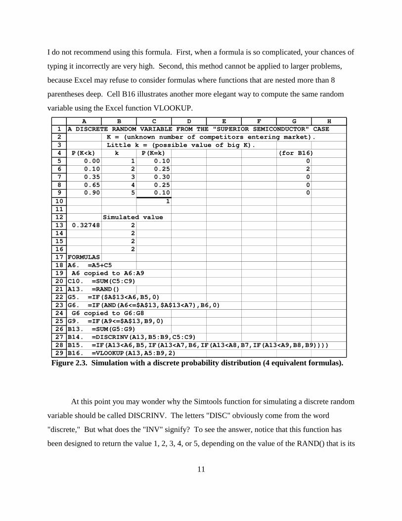
Before stating the Central Limit Theorem, I must introduce the idea of a Normal

probability distribution. In probability theory, the phrase "Normal probability distribution" is

used in a technical sense, which I will emphasize by capitalizing it, referring to a particular

collection of mathematical probability distributions that have some important properties. For any

two numbers µ and F such that F>0, there is precisely-defined Normal probability distribution

that has mean (or expected value) µ and standard deviation F. We will discuss such Normal

27

distributions at length in Chapter 4, but for now it is enough to introduce them by citing a few

basic facts about them.

In an Excel spreadsheet, you can make a random variable that has a Normal probability

distribution with mean µ and standard deviation F by the formula

NORMINV(RAND(),µ,F)

I have tried to suggest here that, once you know how to make a spreadsheet cell that simulates a

given probability distribution, you can learn anything that anybody might want to know about

this distribution by simulating it many times in a spreadsheet. So if you want to know what a

"Normal distribution with mean 100 and standard deviation 20" is like, you should simply copy

the formula

=NORMINV(RAND(),100,20)

into a large range of cells and watch how the values of these cells jump around whenever you

press the recalc key [F9].

Let me give you now a few other useful formulas about Normal distributions. If a

random variable X has a Normal probability distribution with mean µ and standard deviation F

(where µ and F are given numbers such that F>0), then

P(X < µ) = 0.5 = P(X > µ),

P(µ!F < X < µ+F) = 0.683

P(µ!1.96*F < X < µ+1.96*F) = 0.95

P(µ!3*F < X < µ+3*F) = 0.997

That is, a Normal random variable is equally likely to be above or below its mean, it has

probability 0.683 of being less than one standard deviation away from its mean, it has probability

0.997 (almost sure) of being less than 3 standard deviations of its mean. For constructing 95%

confidence intervals, we will use the fact that a Normal random variable has probability 0.95 of

being within 1.96 standard deviations from its mean.

Now we are ready for the remarkable Central Limit Theorem, which tells us Normal

distributions can be used to predict the behavior of sample averages:

Consider the average of n random variables that are drawn independently from a

probability distribution with expected value µ and standard deviation F. This

28

average, as a random variable, has expected value µ, has standard deviation

F'(n^0.5), and has a probability distribution that is approximately Normal.

For example, cell E15 of Figure 2.8 contains the average of n=30 independent random variables

that are drawn from a probability distribution which has expected value µ=3 and standard

deviation F = 1.14. So the Central Limit Theorem tells us that this sample mean should behave

like a random variable that has a Normal distribution where µ=3 is the mean and F'(n^0.5) =

1.14'(30^0.5) = 0.208 is the standard deviation. Such a Normal random variable is entered into

cell H12 of Figure 2.8. If you watch cell H12 and cell E15 through many recalculations, the only

difference in their pattern of behavior that you should observe is that the average in cell E15 is

always a multiple of 1/30. To show more precisely that the sample average in cell E15 has a

probability distribution very close to that of the Normal random variable in cell H12, you could

make a simulation table containing several hundred independently recalculated values of each of

these random variables. Then by separately sorting each column in this simulation table, you

could make a chart that estimates the inverse cumulative distribution of each random variable.

These two curves should be very close.

This Central Limit Theorem is the reason why, of all the formulas that people could

devise for measuring the center and the spread of probability distributions, the expected value

and the standard deviation have been the most useful for statistics. Other probability

distributions that have the same expected value 3 and standard deviation 1.14 could be quite

different in other respects, but the Central Limit Theorem tells us that an average of 30

independent samples from any such distribution would behave almost the same. (For example,

try the probability distribution in which the possible values are 2, 3, and 7, with respective

probabilities P(2)=0.260, P(3)=0.675, and P(7)=0.065.)

Now suppose that we did not know the expected value of K, but we did know that its

standard deviation was F=1.14, and we knew how to simulate K. Then we could look at any

average of n independently simulated values and we could assign 95% probability to the event

that our sample average does not differ from the true expected value by more than

1.96*F'(n^0.5). That is, if we let Y denote the average of our n simulated values, then then

interval from Y !1.96*F'(n^0.5) to Y +1.96*F'(n^0.5) would include the true E(K) withn n

29

probability 0.95. This interval is called a 95% confidence interval. With n=30 and F=1.14, the

radius r (that is, the distance from the center to either end) of this 95% confidence interval would

be

r = 1.96*F'(n^0.5) = 1.96*1.14'(30^0.5) = 0.408.

If we wanted the radius of our 95% confidence interval around the sample mean to be less than

some number r, then we would need to increase the size of our sample so that

1.96*F'(n^0.5) < r, and so n > (1.96*F'r)^2

For example, to make the radius of our 95% confidence interval smaller than 0.05, the

sample size n must be

n > (1.96*F'r)^2 = (1.96*1.14'0.05)^2 = 1997.

Now consider the case where we know how to simulate an unknown quantity but we do

not know how to calculate its expected value or its standard deviation. In this case, where our

confidence-interval formula calls for the unknown probabilistic standard deviation F, we must

replace it by the sample standard deviation that we compute from our simulation data. If the

average of n independent simulations is X and the sample standard deviation is S, then our

estimated 95% confidence interval for the true expected value is from X!1.96*S'(n^0.5) to

X+1.96*S'(n^0.5), where the quantity S'(n^0.5) is our estimated standard deviation of the

sample average. In Figure 2.8, for example, the sample standard deviation S is computed in

cell E16 by the formula =STDEV(A15:C24), the sample size n is computed in cell B10 by the

formula =COUNT(A15:C24), the quantity S'(n^0.5) is computed in cell E17 by the formula

=E16'(B10^0.5)

and then a 95% confidence interval for E(K) is calculated in cells E20 and F20 by the formulas

=E15!1.96*E17 and =E15+1.96*E17

(Recall that E15 is the sample average.)

To say that the interval from E20 to F20 is a 95% confidence interval for the true

expected value is to say that the true expected value of 3 (in cell E8) should be between these two

numbers 95% of the time when the spreadsheet in Figure 2.8 is recalculated many times

independently. You can verify this by watching cell E22 while recalculating. Cell E22 contains

the formula

30

=AND(E20<E8,E8<F20)

and so it should read TRUE about 95% of the time (about 19 times out of 20). (Recall that the

Excel function AND(statement1,statement2) returns the value TRUE if statement1 and

statement2 are both TRUE, and returns FALSE otherwise.)

So based only on the 30 independent simulations shown in Figure 2.8, the formulas in

cells E20 and F20 give us a 95% confidence interval from 2.608 to 3.458, that is 3.033±0.425,

for E(K). If the radius 0.425 seems too large, then we could get a narrower 95% confidence

interval by using a larger sample. If we only knew this estimated sample standard deviation of

1.188, we could estimate that the radius of our 95% confidence interval could be reduced below

0.05 if the sample size n were increased so that 1.96*1.188'(n^0.5) were less than 0.05, which

happens when n is greater than (1.96*1.188'0.05)^2 = 2170.

It is important to understand the difference between cells E16 and E17 in Figure 2.8. The

value of cell E16 is the sample standard deviation STDEV(A15:C24). So E16 is our statistical

estimate of the standard deviation of any one random cell in the range A15:C24. The value of

cell E17 is the sample standard deviation in E16 divided by the square root of the sample size.

So E16 is our estimate of the standard deviation of the random cell E15, which is average of all

the random cells in the range A15:C24. When we recalculate the 30 simulated values in

cells A15:C24, the sample average tends to vary less than any one cell in the sample range,

because when one cell is relatively high there is usually some other relatively low cell to cancel it

out. That is why the standard deviation of the sample average is smaller than the standard

deviation of any one cell in the sample, by a factor of 1'n^0.5.

(You might wonder whether we should broaden our 95% confidence intervals when we

use an estimated sample standard deviation instead of the true standard deviation. The answer is

that we should, but the adjustments are relatively minor unless the sample size is small. The

corrected formula is based on something that statisticians call a T-distribution. When the sample

size n is small, we should replace the constant 1.96 in our 95% confidence formulas by the value

of the Excel formula TINV(0.05,n!1). When n is 30, this value is 2.045. As the sample size n

increases, the value of TINV(0.05,n!1) rapidly approaches 1.96, and so we will not worry about

this T-adjustment in this book.)

31

Another application of the Central Limit Theorem can also be used to tell us something

about the accuracy of our statistical estimates of points on the inverse cumulative probability

curve. Suppose that X is a random variable with a probability distribution that we know how to

simulate, but we do not know how to directly compute its cumulative probability curve. For any

number y, let Q (y) denote the percentage of our sample that is less than y, when we get a samplen

of n independent values drawn from the probability distribution of X. Then we should use Q (y)n

as our estimate of P(X<y). But how good is this estimate? When n is large, Q (y) is a randomn

variable with an approximately Normal distribution, its expected value is P(X<y), and its

standard deviation is (P(X<y)*(1!P(X<y))'n)^0.5. But (p*(1!p))^0.5 # 0.5 for any probability

p, and so the standard deviation of Q (y) is always less than 0.5'(n^0.5), and multiplying thisn

standard deviation by 1.96 yields a number slightly less than 1'n^0.5. Thus, around any point

(Q (y),y) in an estimated inverse cumulative probability curve like Figure 2.7, we could put an

horizontal confidence interval over the cumulative probabilities from Q (y)!1'n^0.5 ton

Q (y)+1'n^0.5, and this interval would have a probability greater than 95% of including the truen

cumulative probability at y. When n is 400, for example, the radius of this cumulative-

probability interval around Q (y) is 1'n^0.5 = 1'20 = 0.05. If we wanted to reduce the radius ofn

this 95%-confidence interval below 0.02, then we would increase the sample size to

1'0.02^2 = 2500.

2.7 Decision criteria

We have used the Superior Semiconductor case as an example to introduce basic ideas of

probability and statistics. But after all these ideas have been introduced, we are still left with a

decision problem. On the basis of our analysis of the uncertainty in this situation, should we

recommend that Superior Semiconductors introduce the new T-regulator product or not? To

answer this question, we need some fundamental assumption about what determines an optimal

decision under uncertainty. The assumption that we will usually apply in this course is the

criterion of expected value maximization (or the expected value criterion).

Any quantitative decision analysis must involve some numerical measure of payoff, such

that increasing the decision-maker's payoff is considered an improvement. For most economic

32

decision problems, net monetary returns or profit (or the present-discounted value of future

profit) may be identified as the payoff that the decision-maker wants to increase whenever

possible. But in situations with uncertainty, we may not know whether a particular decision (like

that of introducing the new T-regulator product) would increase or decrease the decision-maker's

payoff. The criterion of expected value maximization asserts that, among the various alternatives

that are available to a decision-maker, the optimal decision is the one that yields the highest

expected value of the decision-maker's payoff.

So if we take Superior Semiconductor's profit to be the measure of "payoff" in this

decision problem, then the optimal decision can be identified simply by computing the expected

value of Superior Semiconductor's profit from the proposed new product. As we have seen, this

expected value is

E(Profit) = 0.10*24 +0.25*7.33 + 0.30*(!1) + 0.25*(!6) + 0.10*(!9.33) = 1.5

The alternative of not introducing the new product generates an expected profit of 0, of course.

So by the criterion of expected value maximization, Superior Semiconductor should introduce

the new product, because 1.5 > 0.

The expected value formula has many good properties to recommend it as a criterion for

decision-making under uncertainty. It takes account of all possible outcomes in a sensible way,

and it is more sensitive to outcomes that are more likely. The argument for expected value

maximization is particularly compelling in games that can be repeated. If we know that we will

repeat a given type of decision problem many times, with new payoffs from each repetition being

added to the payoffs from previous rounds, but with the new outcome being determined

independently each time, then a strategy of choosing the alternative that yields the highest

expected value will almost surely maximize our long-term total payoff, by the law of large

numbers.

This expected-value criterion may be interpreted to mean that all we should care about is

the expected value of some appropriately measured payoff. But this interpretation can lead to

trouble if the words "of ... payoff" are forgotten. If you thought that our expected-value criterion

meant that we should only care about the expected number of competitors, then you would act as

though the number of competitors would be 3, in which case profit would be !1, and your

12345678910111213141516171819202122232425262728293031323334353637383940414243

A B C D E F G HSUPERIOR SEMICONDUCTOR (A) (B) 26 FixedCost

100 MarketValueLet K = (unknown number of competitors entering market)Probability distribution of K

k P(K=k) Profit ($millions) if k=#compet'rs1 0.10 24.002 0.25 7.33 Measuring risk tolerance3 0.30 -1.00 High$ 20.004 0.25 -6.00 Low$ -10.005 0.10 -9.33 Assessed value$ 2.00

RiskTolerance 36.4891Computations from probability distribution

E(K) E(Profit) CertaintyEquivalent3 1.5 0.423906

Simulation modelK Profit

5 -9.33

Statistics from simulations:1.83458 E(Profit) est'd from SimTable

9.611946 Stdev(Profit) est'd from SimTable-9.33333 5% cumulative-probability level

401 Sample size Estimated CE 0.69603995% conf.intl for E(Profit)

Sim'd profit 0.8937847 2.775376SimTable -9.33

0 -6 FORMULAS0.0025 -9.33333 E6. =$E$2/(1+B6)-$E$10.005 -6 E6 copied to E6:E10 and E18

0.0075 -6 B14. =SUMPRODUCT(B6:B10,$C$6:$C$10)0.01 -1 E14. =SUMPRODUCT(E6:E10,$C$6:$C$10)

0.0125 -6 B18. =DISCRINV(RAND(),B6:B10,C6:C10)0.015 -6 B27. =E18

0.0175 -1 B21. =AVERAGE(B28:B428)0.02 -1 B22. =STDEV(B28:B428)

0.0225 -1 B23. =PERCENTILE(B28:B428,0.05)0.025 7.333333 B24. =COUNT(B28:B428)

0.0275 -1 E26. =B21-1.96*B22/(B24^0.5)0.03 24 F26. =B21+1.96*B22/(B24^0.5)

0.0325 -1 H11. =RISKTOL(H8,H9,H10)0.035 -1 H14. =CEPR(E6:E10,C6:C10,H11)

0.0375 -9.33333 H24. =CE(B28:B428,H11)

33

Figure 2.9. Analysis of Superior Semiconductor case.

recommendation would be to not introduce the new product. The error here is to compute the

expected value of the wrong random variable (not payoff), and then to try to compute an

expected payoff from it according to the fallacy of averages (as discussed in Section 2.4).

34

Figure 2.9 shows a decision analysis of the Superior Semiconductor case. In cell E14, the

expected value is profit is calculated directly from the probability distribution. Under the

expected value criterion, this positive expected value in E14 tells us that we should recommend

the new product. But to illustrate what we would do if we could not compute expected profit

directly from the probability distribution, the spreadsheet also contains a table of 401

independent simulations of the unknown profit, and the average of these profits is exhibited in

cell B21 as an estimator of the expected profit. Even if we could not see the true expected value

in cell E14, our simulation data is strong enough to support reasonable confidence that the

expected value is greater than 0, because we find a positive lower bound (0.8937) in the 95%

confidence interval for expected profit that is computed in cells E26 and F26.

But now, having advocated the expected value criterion, I must now admit that it is often

not fully satisfactory as a basis for decision-making. In practice, people often prefer decision

alternatives that yield lower expected profits, when the alternatives that yield higher expected

profits are also more risky. People who feel this way are risk averse. Because most people

express attitudes of risk aversion at least some of the time, a serious decision analysis should go

beyond simply reporting expected payoff values, and should also report some measures of the

risks associated with the alternatives that are being considering.

As we have seen, the standard deviation is often used as a measure of the spread of likely

outcomes of an unknown quantity, and so the standard deviation of profit may be used as a

measure of risk. Thus, cell B22 in Figure 2.9 estimates the standard deviation of profit from the

proposed new product in this case. The large size of this sample standard deviation

(9.61 $million, much larger than the expected value) is a strong indication that this new product

should be seen as a very risky.

Another measure of risk that has gained popularity in recent years is called value at risk.

The value at risk is defined to be the level of net profit that has some small pre-specified

cumulative probability, often taken to be 0.05, so that the probability of profit being below this

level is not more than 1/20. So cell B23 in Figure 2.9 estimates the profit level that has 5%

cumulative probability from our simulation data in B28:B428, using the formula

-10

-5

0

5

10

15

20

25

0 0.1 0.2 0.3 0.4 0.5 0.6 0.7 0.8 0.9 1

Cumulative probability

Pro

fit(

$mill

ions

)

35

Figure 2.10. Cumulative risk profile, from simulation data.

=PERCENTILE(B28:B428,0.05).

The cumulative risk profile for a decision may be defined as the inverse cumulative

probability distribution of the payoff that would result from this decision. Figure 2.10 shows the

cumulative risk profile for the decision to introduce the new product in this case. This

cumulative risk profile was made from the simulation table in Figure 2.9. (First the simulated

profit data in cells B28:B428 were sorted by Excel's Data:Sort command, and then these sorted

profit values were plotted on the vertical axis of an XY-chart, with the percentile index in cells

A28:A428 plotted on the horizontal axis.) Notice that this cumulative risk profile contains all the

information about the value at risk, for any probability level. By definition, the value at risk for

the cumulative-probability level 0.05 is just the height of the cumulative risk profile above 0.05

on the horizontal cumulative-probability axis. So the cumulative risk profile may give the most

complete overall picture of the risks associated with a decision.

More generally, the limitations of the expected value maximization as a criterion for

decision-making have been addressed by two important theories of economic decision-making:

36

utility theory and arbitrage-pricing theory. Utility theory is about decision-making by risk-averse

individuals. Arbitrage-pricing theory is about decision-making for publicly held corporations,

which may be owned by people who have different attitudes towards risks and different beliefs

about the probabilities of various events. Utility theory will be discussed in Chapter 3 of this

book, and arbitrage-pricing theory will be discussed in Sections 8.3 and 8.4 of Chapter 8. But

each of these theories turns out to be mathematically equivalent to a simple extension of the

expected value criterion. In utility theory, the expected value criterion is extended by introducing

a new way of measuring payoffs, called a utility function, that takes account of the decision-

maker's personal willingness to take risks. In arbitrage pricing theory, the expected value

criterion is extended by introducing a new way of measuring probabilities, called market-adjusted

probabilities, that takes account of asset-pricing in financial markets. Thus, the techniques that

we have developed in this chapter for estimating expected values will also be applicable to more

sophisticated theories of individual and corporate decision-making.

(For a preview of the results of utility theory, you can look in column H of Figure 2.9

above. In Part B of the Superior Semiconductor case, the decision-maker will remark that a

simple gamble that could generate either a profit of $20 million or a loss of $10 million for

Superior Semiconductor, each with probability 1/2, may be just as good for the company as

$2 million for sure. Based on this assessment, cell H11 in Figure 2.9 applies a Simtools function

called RISKTOL to compute a measure of the company's "risk tolerance." Then with this

measure of the company's "risk tolerance," cell H14 applies a Simtools function called CEPR to

compute a risk-adjusted "certainty equivalent" value of the T-regulator project, using the

probability distribution of its profits. Cell H24 applies another Simtools function called CE to

estimate this same "certainty equivalent" value using simulation data. The meanings of these

mysterious functions and quantities will be discussed at length in Chapter 3.)

2.8 Multiple random variables

We have been considering a simple example with just one random variable, because this

simplicity allowed us to compare our first estimates from simulation data to the actual quantites

being estimated. But now that we understand how simulation works, we can begin applying it to

37

more interesting problems that have many random variables, where probabilities, expected

values, and standard deviations may be very difficult to calculate from probability distributions,

so that simulation analysis becomes our best technique.

For example, Figure 2.11 shows an analysis of a more complicated version of the

Superior Semiconductor case where the development cost and total market value are also

unknown quantities. Instead of assuming that development cost D is 26 $million for sure, it is

assumed now that the development cost could be 20, 26, 30, or 34 $million with probabilities

0.2, 0.5, 0.2, and 0.1 respectively. Instead of assuming that the total market value M is 100

$million for sure, it is assumed now that the development cost could be 70, 100, 120, or 150

$million with probabilities 0.3, 0.4, 0.2, and 0.1 respectively. The number of competitors K as

before could be 1, 2, 3, 4, or 5, with probabilities 0.1, 0.25, 0.3, 0.25, and 0.1 respectively. The

profit depends on these quantities by the formula Y = M'(1+K)!D because we assume that the

total market value will be divided equally among Superior Semiconductors and its K

competitors.

Cells A11, D11, and G11 in Figure 2.11 contain random variables (made with

DISCRINV) that simulate the number of competitors, the development cost, and the total market

value for Superior Semiconductor's new T-regulator device. The spreadsheet uses an assumption

that these unknown quantities are independent (that is, learning about any one of them would not

influence our beliefs about the others), because the three random variables in cells A11, D11 and

G11 are independently driven by their own separate RANDs. Then profit is calculated in cell

B13 by the formula =G11/(1+A11)-D11.

Profit data from 501 simulations of this model are stored in B14:B514. The sample

average is calculated in D14, and a 95% confidence interval for the true expected profit is

calculated around this sample average in cells G14 and H14. Based on this analysis, it appears

that the strategy of introducing the new T-regulator product can be recommended under the

expected value criterion, but a larger simulation table may be needed to be more confident about

the positivity of expected profit. The risks appear even greater in this model, as evidenced by a

higher standard deviation (in cell D15) and a lower 0.05 cumulative-probability profit level (in

cell D16), compared to the analogous statistics in Figure 2.9.

12345678910111213141516171819202122232425262728293031323334353637383940414243444546

A B C D E F G H I#Competitors Dev't cost Total marketvalue proby value proby value proby

1 0.1 20 0.2 70 0.32 0.25 26 0.5 100 0.43 0.3 30 0.2 120 0.24 0.25 34 0.1 150 0.15 0.1 1 1

1SIMULATION MODEL#Competitors Development cost Total market$

3 20 100Profit

SimTable 5 Ests from SimTable 95% ConfIntl for EProfit0 -22.333 1.11477 E(Profit) -0.0069 2.23647

0.002 -20 12.8097 Stdev(Proft)0.004 -20 -14.333 5%ile Profit Sample size0.006 -20 0.582 P(Profit<0) 5010.008 -20 FORMULAS0.01 -20 B8. =SUM(B3:B7)

0.012 -18.333 E7. =SUM(E3:E6) E7 copied to H70.014 -18.333 A11. =DISCRINV(RAND(),A3:A7,B3:B7)0.016 -18.333 D11. =DISCRINV(RAND(),D3:D6,E3:E6)0.018 -18.333 G11. =DISCRINV(RAND(),G3:G6,H3:H6)0.02 -18.333 B13. =G11/(1+A11)-D11

0.022 -18.333 D14. =AVERAGE(B14:B514)0.024 -16.5 D15. =STDEV(B14:B514)0.026 -16.5 D16. =PERCENTILE(B14:B514,0.05)0.028 -16.5 D17. =PERCENTRANK(B14:B514,0)0.03 -16.5 H17. =COUNT(B14:B514)

0.032 -16 G14. =D14-1.96*D15/H17^0.50.034 -16 H14. =D14+1.96*D15/H17^0.50.036 -160.038 -160.04 -16

0.042 -160.044 -160.046 -160.048 -14.3330.05 -14.333

0.052 -14.3330.054 -140.056 -140.058 -140.06 -14

0.062 -14 Data in B14:B514 is sorted for chart.0.064 -14 Chart plots (A14:A514,B14:B514).

Cumulative risk profile

-30

-20-10

010

2030

40

50

60

0 0.1 0.2 0.3 0.4 0.5 0.6 0.7 0.8 0.9 1

Cumulative probabilty

Prof

it($

mill

ions

)

38

Figure 2.11. A simulation model with three random variables affecting profit.

39

A fuller picture of the probability distribution of profit in this example is offered by the

cumulative risk profile, which plots the sorted simulation data in B14:B514 on the vertical axis

against the simulation table's percentile index (in A14:A514) on the horizontal axis. The Excel

functions PERCENTILE and PERCENTRANK are also used in Figure 2.11 to extract numerical

information about this distribution. To estimate the cumulative probability of profit at $0, the

fraction of the simulated profits in B14:B514 that are less than $0 is computed in cell D17 by the

formula

=PERCENTRANK(B14:B514,0).

To estimate the profit value that has cumulative probability 0.05, cell D16 finds the value that is

greater than 5% of the simulated profits, using the formula

=PERCENTILE(B14:B514,0.05).

2.9 Summary

In this chapter, we focused on a simple decision problem involving an unknown quantity

that has only finitely many possible values. In this context, we introduced some basic concepts

for describing discrete probability distributions: the expected value or mean of the distribution,

the standard deviation and the variance, and cumulative probability charts. We saw how to make

a random variable with any given probability distribution by using the inverse cumulative-

probability function with a RAND() as input. The Simtools function DISCRINV was introduced

to facilitate such simulations.

We then introduced techniques for estimating expected values, standard deviations, and

cumulative probabilities from simulation data, using the law of large numbers for assurance that

these estimates are very likely to be quite accurate if the sample size is very large. For a more

precise assessment of the accuracy of the sample average as an estimate for an unknown expected

value, we introduced Normal distributions and the Central Limit Theorem. We learned that a

sample average, as a random variable, has a standard deviation that is inversely proportional to

the square root of the sample size. We then saw how to compute a 95% confidence interval for

the expected value of a random variable, using simulation data.

40

Finally, criteria for optimal decision-making were discussed, beginning with the basic

concept of expected value maximization. The expected value of monetary income or some other

suitably-measured payoff quantity was recommended as the best single number to guide

decision-making under uncertainty. The standard deviation of payoff, the value at risk (for some

pre-specified cumulative-probability level), and the entire cumulative risk profile were

recommended as also worth reporting in a decision analysis, to better describe the levels of risk

entailed by different decision alternatives.

Excel functions used in this chapter include AND, NORMINV, STDEV, and

SUMPRODUCT. Simtools functions introduced in this chapter include DISCRINV and

STDEVPR. We also used the Data:Sort and Insert:Chart:XY-Scatter commands to make inverse

cumulative charts from simulation data.

EXERCISES

1. Let X denote an unknown quantity that has three possible values: 2, 3, and 7, and suppose thattheir probabilities are P(X=2) = 0.260, P(X=3) = 0.675, P(X=7) = 0.065.Let Y denote another unknown quantity that has three possible values: !1, 3, and 4, and supposethat their probabilities are P(Y=!1) = 0.065, P(Y=3) = 0.675, P(Y=4) = 0.260.(a) Compute E(X), Stdev(X), E(Y) and Stdev(Y).(b) According to the central limit theorem, an average of 36 random variables drawn from theprobability distribution of X should have approximately what probability distribution? (Be sureto specify the mean and standard deviation.)(c) In a spreadsheet, make a simulation table that tabulates values of five random variables asfollows:the first is a single cell that simulates X,the second is a single cell that simulates Y,the third is an average of 36 cells independently drawn from the probability distribution of X,the fourth is an average of 36 cells independently drawn from the probability distribution of Y,the fifth is a single random cell drawn from the probability distribution that you predicted in (b).Include at least 400 data rows in your simulation table. (This calculation may take a few minuteson older computers.)(d) Using your simulation table in (c), compute the sample mean and standard deviation for eachof the five random variables, and make an XY-chart that estimates the (inverse) cumulativedistribution for these five random variables. (Hint on charting keystrokes: You can separatelysort each of your five columns of simulation data, then select the percentile index and five sorteddata columns in the simulation table, and insert an XY-chart.)

41

2. In a simulation table with data from 400 independent simulations of a random variable W, thesample mean is 220.12, and the sample standard deviation is 191.63.(a) Estimate the standard deviation of the sample mean when the sample size is 400.(b) Based on this data, compute a 95% confidence interval for the true expected value of thisrandom variable E(W).(c) Suppose that we want to make a new table of simulation data which will generate a 95%confidence interval for E(W) that has a radius of about 5. How large should this new simulationtable be? (That is, how many independent simulations should it include?)

3. What is the discrete probability distribution of the random variable that would be generated byeach of the following Excel formulas? Check your answer by a large simulation.(a) =IF(RAND()>0.3,2,0)+IF(RAND()>0.6,3,0)(b) =IF(AND(0.3<RAND(),RAND()<0.4),1,0)(c) =IF(RAND()<0.6,IF(RAND()<0.5,1,2),3)(d) How would your answers change if we entered =RAND() into cell A1 and we replaced everyRAND() in the above formulas by a reference to cell A1?

4. Acme Widget Company has substantial uncertainty about many factors that will affect itsprofit from selling widgets next year. Acme's director of marketing estimates that the totaldemand for widgets (sold by all firms in the market) may be 60,000 or 70,000 or 80,000 widgetsnext year, and the probabilities of these three possibilities are 0.2, 0.6, and 0.2 respectively.Acme's share of this total market for widgets next year may be 0.15 or 0.20 or 0.25 or 0.30, withprobabilities 0.2, 0.3, 0.3, and 0.2 respectively. The price of widgets next year may be $90 or$100 or $110 per widget, with probabilities 0.2, 0.7, and 0.1 respectively.Suppose that, after the assembly line is set up, Acme can produce its widgets as customers orderthem, and so Acme's production quantity will equal its demand. Acme's costs can be separatedinto two parts: a fixed cost of setting up the assembly line, and a variable cost per widgetproduced. Acme's production manager estimates that the fixed cost may be $450,000 or$500,000 or $550,000 or $600,000, each with probability 0.25. The variable cost per widget maybe either $50 per widget, with probability 0.6, or $60 per widget, with probability 0.4.(a) Make a spreadsheet simulation model to represent this situation, assuming that theseunknown quantities are independent.(b) Generate a large table of simulated profits, and compute a 95% confidence interval forAcme's expected profit from widget production next year. Make sure that our simulation table islarge enough that the radius of your 95% confidence interval for Acme's expected profit is lessthan $10,000. (That is, get a 95% confidence interval of the form m±r where r < 10,000.)(c) Using the simulation data from part (b) also estimate:

(i) the standard deviation of Acme's profit next year,(ii) the probability of Acme's profit next year being negative,(iii) the median level of Acme's profit next year,(iv) the level of Acme's profit next year that has cumulative probability 0.75.

(d) Based on the simulation data from part (b), make a chart showing the cumulative risk profilefor Acme's profit next year.