Chapter 2 covers :
62
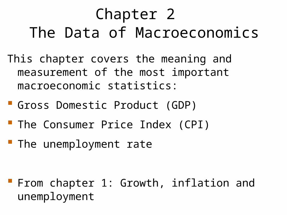
Chapter 2 : The Data of Macroeconomics This chapter covers the meaning and measurement of the most important macroeconomic statistics: Gross Domestic Product (GDP) The Consumer Price Index (CPI) The unemployment rate From chapter 1: Growth, inflation and unemployment
description
Chapter 2 covers :. …the meaning and measurement of the most important macroeconomic statistics: Gross Domestic Product (GDP) The Consumer Price Index (CPI) The unemployment rate. Gross Domestic Product: Expenditure and Income. Two definitions: - PowerPoint PPT Presentation
Transcript of Chapter 2 covers :
Chapter 2 :The Data of Macroeconomics
This chapter covers the meaning and measurement of the most important macroeconomic statistics:
Gross Domestic Product (GDP)
The Consumer Price Index (CPI)
The unemployment rate
From chapter 1: Growth, inflation and unemployment
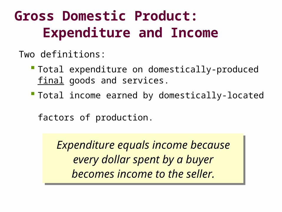
Gross Domestic Product: Expenditure and Income
Two definitions:
Total expenditure on domestically-produced final goods and services.
Total income earned by domestically-located factors of production.
Expenditure equals income because every dollar spent by a buyer becomes income to the seller.
Expenditure equals income because every dollar spent by a buyer becomes income to the seller.

The Circular Flow
Households Firms
Goods
Labor
Expenditure ($)
Income ($)

Value added
Value added: The value of output minus the value of the intermediate goods used to produce that output

Stages of Production
Example: Production of Notebook Paper
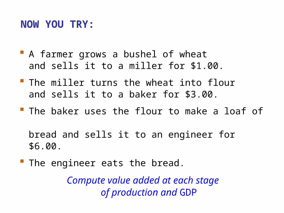
NOW YOU TRY:
A farmer grows a bushel of wheat and sells it to a miller for $1.00.
The miller turns the wheat into flour and sells it to a baker for $3.00.
The baker uses the flour to make a loaf of bread and sells it to an engineer for $6.00.
The engineer eats the bread.
Compute value added at each stage of production and GDP
Final goods, value added, and GDP
GDP = value of final goods produced
= sum of value added at all stages of production.
= income earned by factors of production
The value of the final goods already includes the value of the intermediate goods, so including intermediate and final goods in GDP would be double-counting.
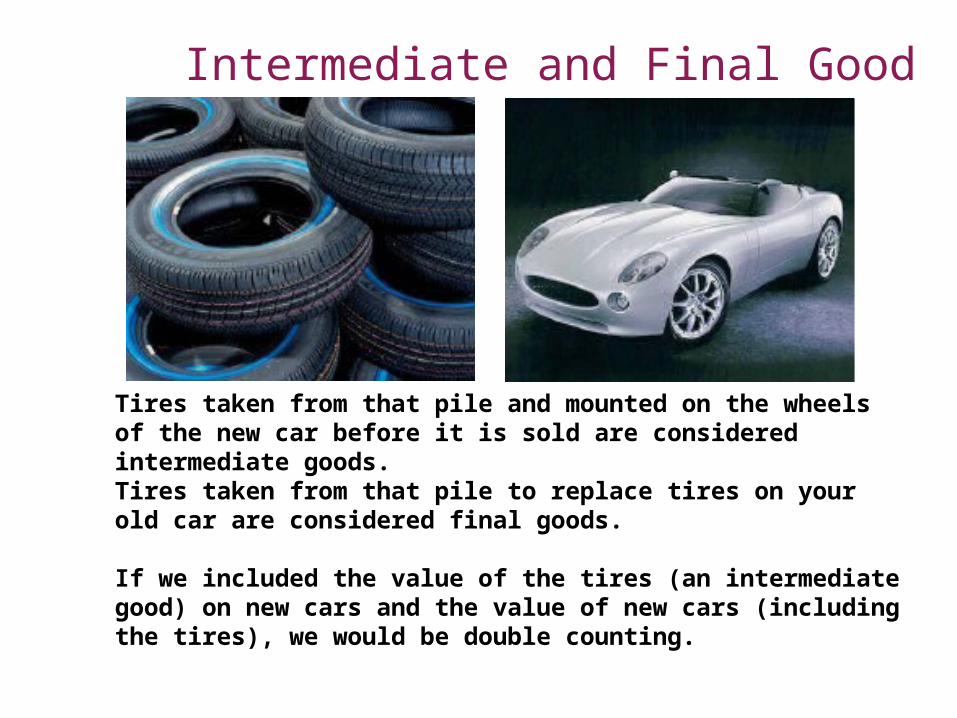
Intermediate and Final Good
Tires taken from that pile and mounted on the wheels of the new car before it is sold are considered intermediate goods.Tires taken from that pile to replace tires on your old car are considered final goods.
If we included the value of the tires (an intermediate good) on new cars and the value of new cars (including the tires), we would be double counting.
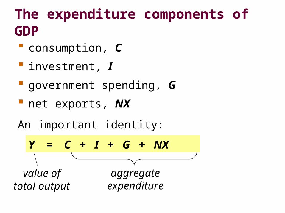
The expenditure components of GDP consumption, C
investment, I
government spending, G
net exports, NX
An important identity:
Y = C + I + G + NX
aggregate expenditure
value of total output
Consumption (C)
durable goods last a long time e.g., cars, home appliances
nondurable goodslast a short time e.g., food, clothing
serviceswork done for consumers e.g., dry cleaning, air travel
definition: The value of all goods and services bought by households. Includes:
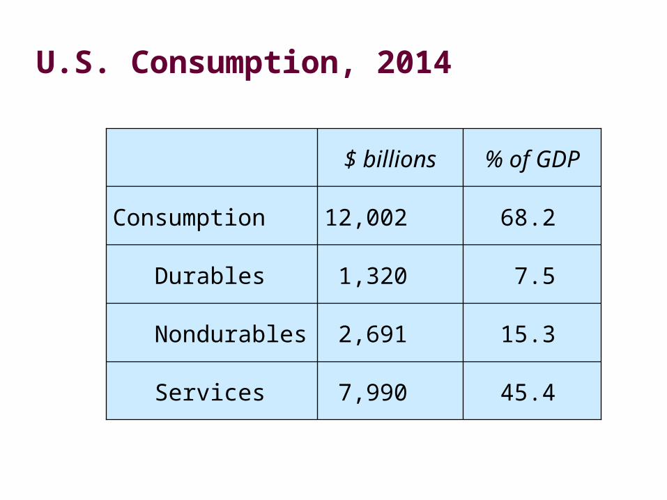
U.S. Consumption, 2014
45.4
15.3
7.5
68.2
7,990
2,691
1,320
12,002
Services
Nondurables
Durables
Consumption
% of GDP$ billions
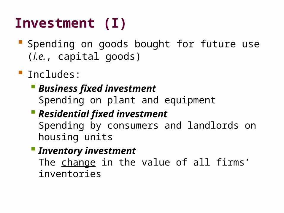
Investment (I)
Spending on goods bought for future use (i.e., capital goods)
Includes: Business fixed investment
Spending on plant and equipment Residential fixed investment
Spending by consumers and landlords on housing units
Inventory investmentThe change in the value of all firms’ inventories
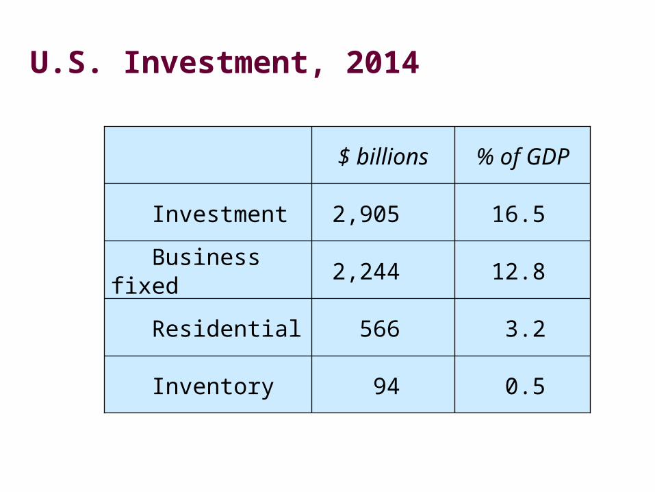
U.S. Investment, 2014
0.5
3.2
12.8
16.5
94
566
2,244
2,905
Inventory
Residential
Business fixed
Investment
% of GDP$ billions
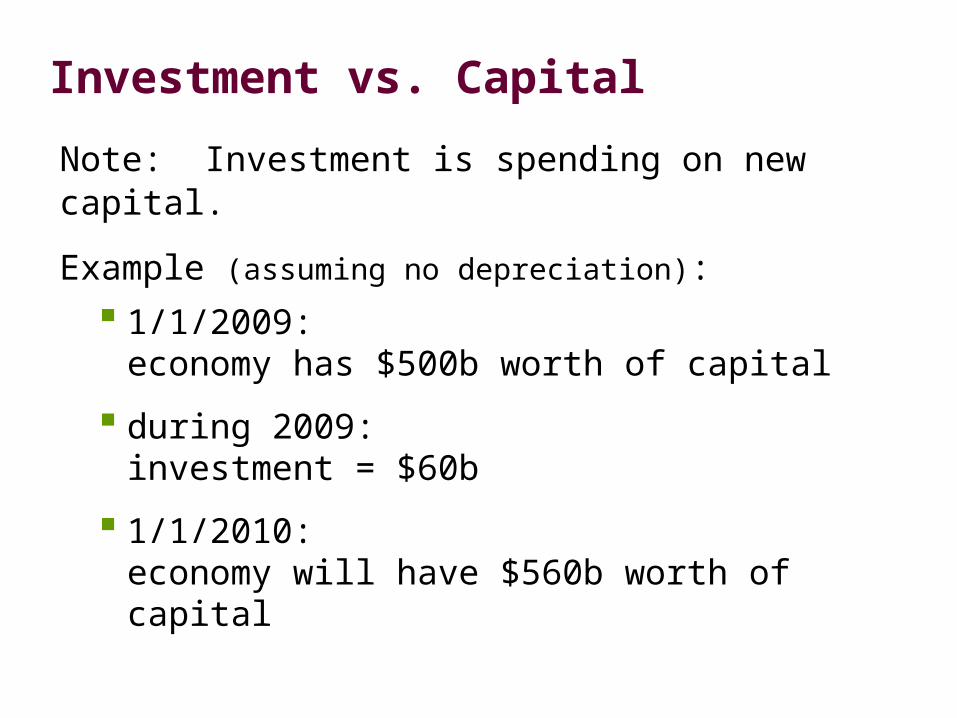
Investment vs. Capital
Note: Investment is spending on new capital.
Example (assuming no depreciation):
1/1/2009: economy has $500b worth of capital
during 2009:investment = $60b
1/1/2010: economy will have $560b worth of capital
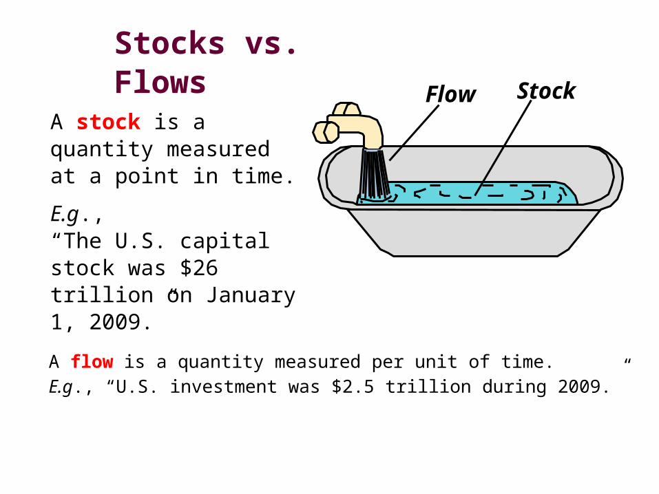
Stocks vs. Flows
A flow is a quantity measured per unit of time. E.g., “U.S. investment was $2.5 trillion during 2009.”
Flow Stock
A stock is a quantity measured at a point in time.
E.g., “The U.S. capital stock was $26 trillion on January 1, 2009.”
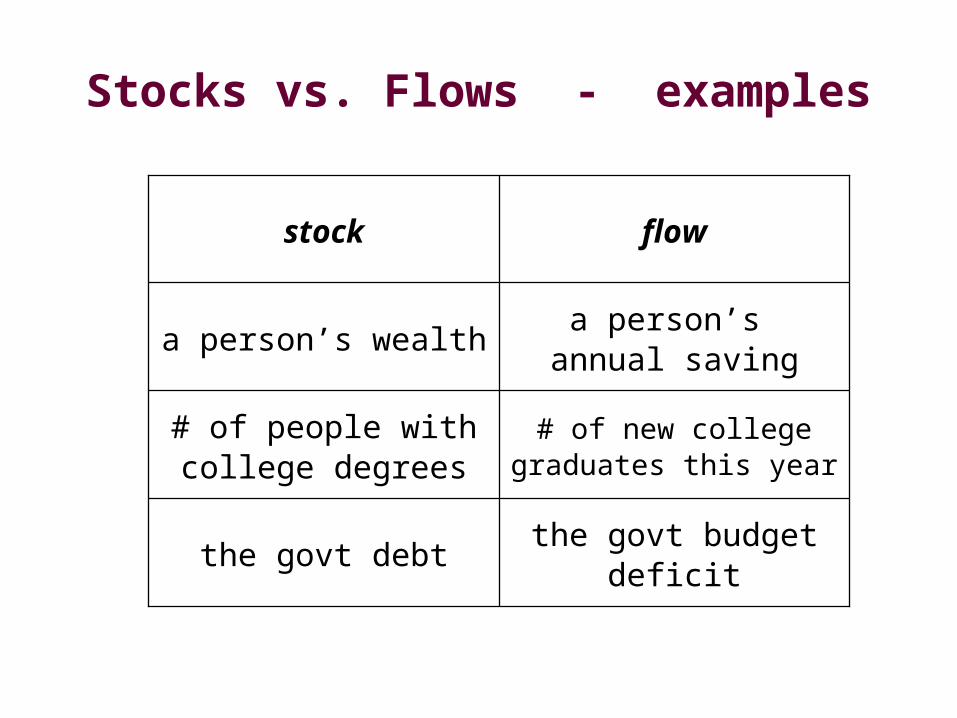
Stocks vs. Flows - examples
the govt budget deficitthe govt debt
# of new college graduates this year
# of people with college degrees
a person’s annual saving
a person’s wealth
flowstock
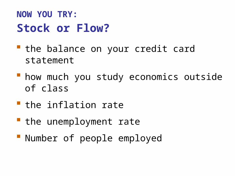
NOW YOU TRY:
Stock or Flow?
the balance on your credit card statement
how much you study economics outside of class
the inflation rate
the unemployment rate
Number of people employed
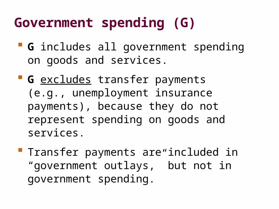
Government spending (G)
G includes all government spending on goods and services.
G excludes transfer payments (e.g., unemployment insurance payments), because they do not represent spending on goods and services.
Transfer payments are included in “government outlays,” but not in government spending.
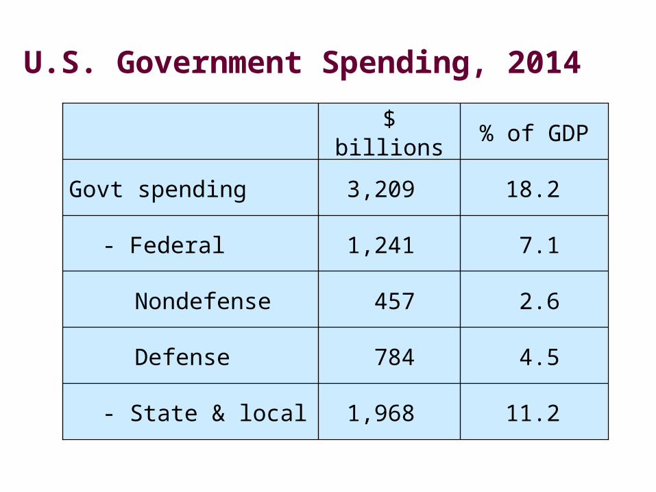
U.S. Government Spending, 2014
- Federal
18.23,209Govt spending
- State & local
Defense
7.1
11.2
4.5
2.6
1,241
1,968
784
457Nondefense
% of GDP$ billions
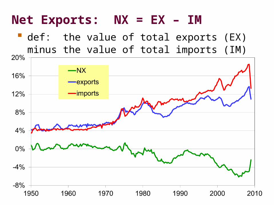
Net Exports: NX = EX – IM def: the value of total exports (EX) minus the value
of total imports (IM)
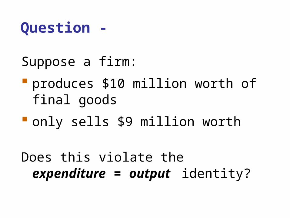
Question -
Suppose a firm:
produces $10 million worth of final goods
only sells $9 million worth
Does this violate the expenditure = output identity?
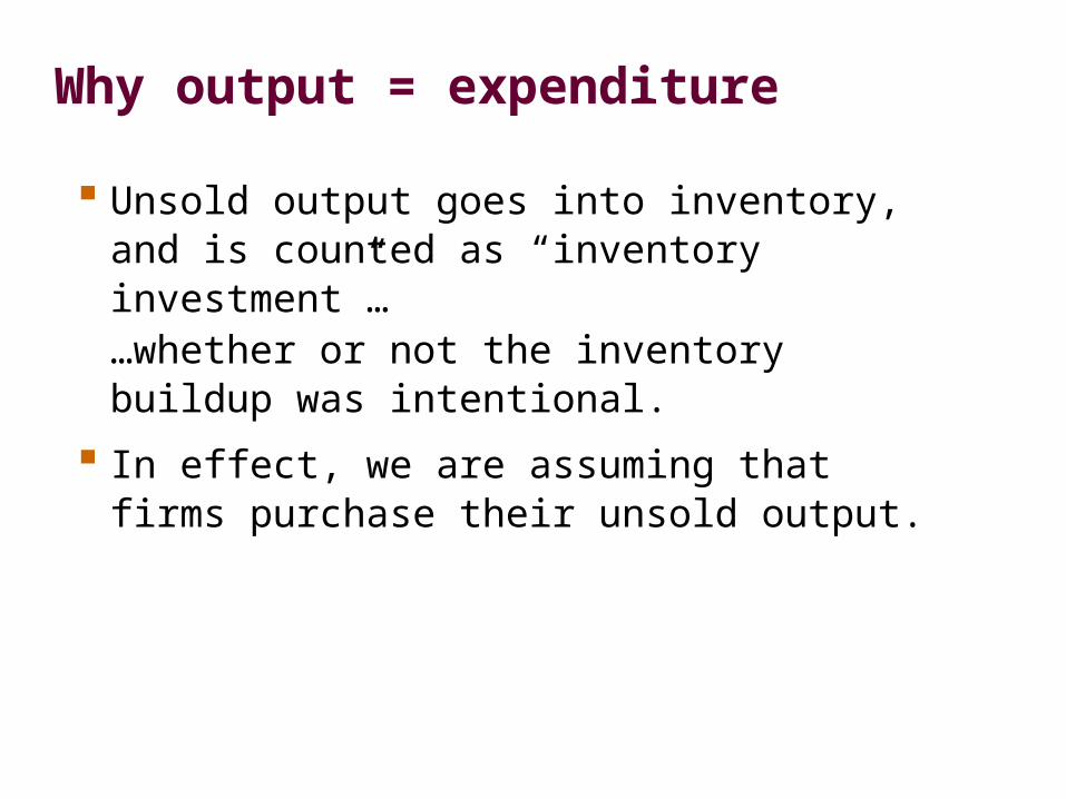
Why output = expenditure
Unsold output goes into inventory, and is counted as “inventory investment”……whether or not the inventory buildup was intentional.
In effect, we are assuming that firms purchase their unsold output.
GDP: An Important and versatile concept
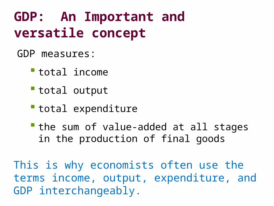
GDP measures:
total income
total output
total expenditure
the sum of value-added at all stages in the production of final goods
This is why economists often use the terms income, output, expenditure, and GDP interchangeably.
GNP vs. GDP
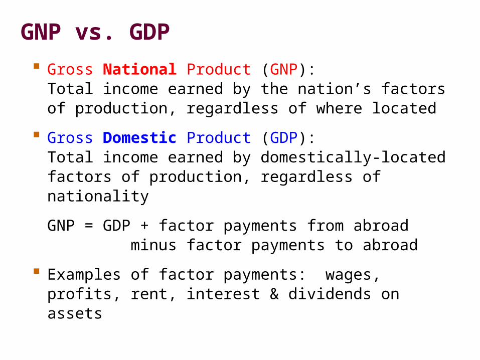
Gross National Product (GNP): Total income earned by the nation’s factors of production, regardless of where located
Gross Domestic Product (GDP):Total income earned by domestically-located factors of production, regardless of nationality
GNP = GDP + factor payments from abroad minus factor payments to
abroad
Examples of factor payments: wages, profits, rent, interest & dividends on assets
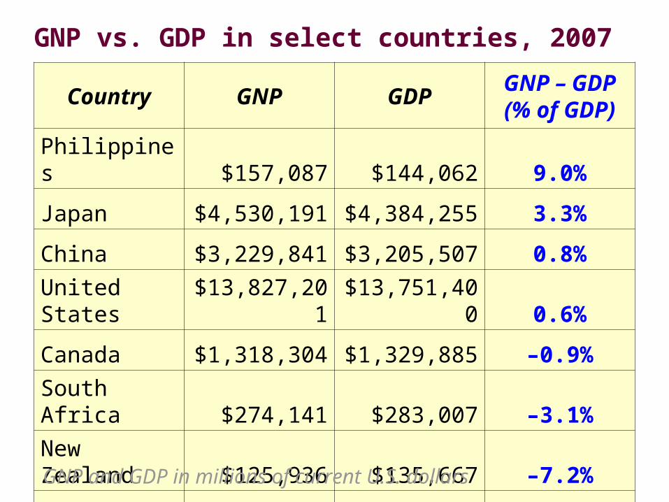
GNP vs. GDP in select countries, 2007
Country GNP GDPGNP – GDP (% of GDP)
Philippines $157,087 $144,062 9.0%
Japan $4,530,191 $4,384,255 3.3%
China $3,229,841 $3,205,507 0.8%
United States $13,827,201 $13,751,400 0.6%
Canada $1,318,304 $1,329,885 –0.9%
South Africa $274,141 $283,007 –3.1%
New Zealand $125,936 $135,667 –7.2%
Peru $98,625 $107,297 –8.1%
GNP and GDP in millions of current U.S. dollars
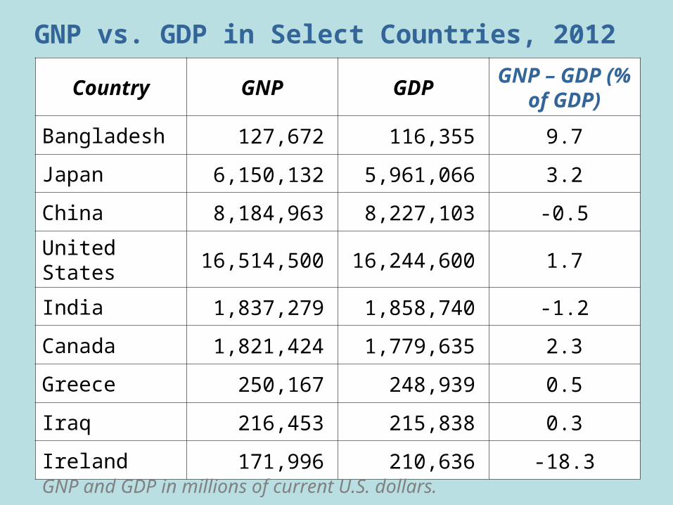
GNP vs. GDP in Select Countries, 2012
Country GNP GDPGNP – GDP (% of GDP)
Bangladesh 127,672 116,355 9.7
Japan 6,150,132 5,961,066 3.2
China 8,184,963 8,227,103 -0.5
United States 16,514,500 16,244,600 1.7
India 1,837,279 1,858,740 -1.2
Canada 1,821,424 1,779,635 2.3
Greece 250,167 248,939 0.5
Iraq 216,453 215,838 0.3
Ireland 171,996 210,636 -18.3
GNP and GDP in millions of current U.S. dollars.
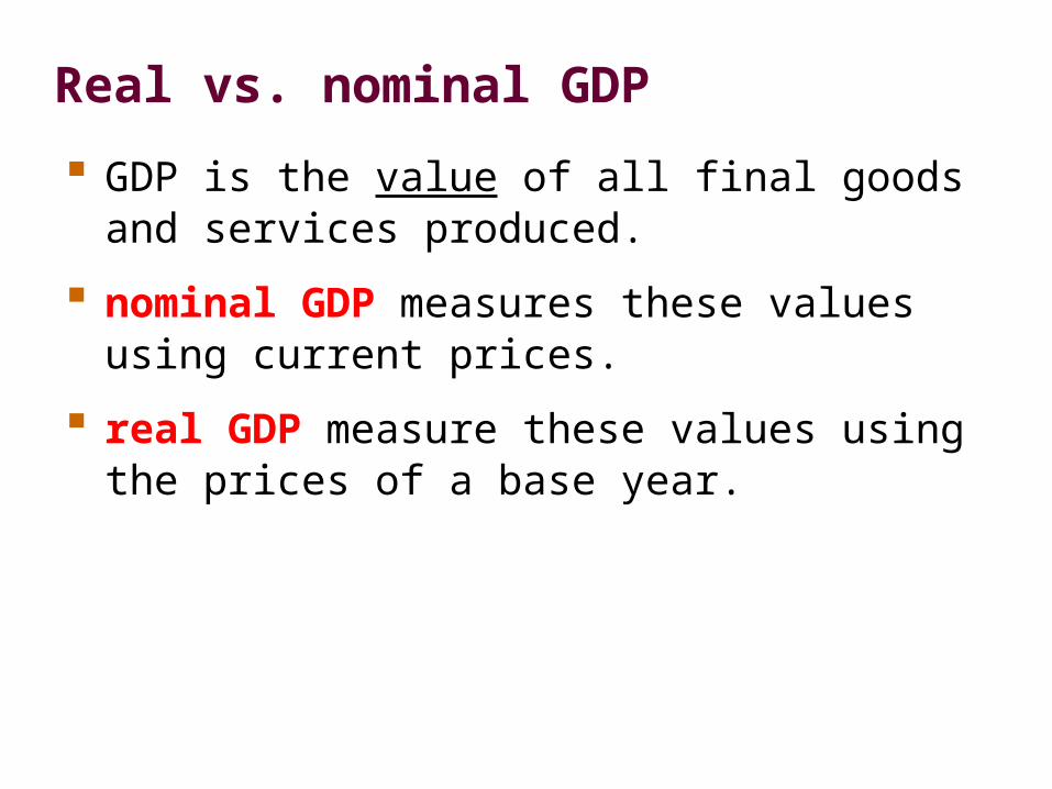
Real vs. nominal GDP
GDP is the value of all final goods and services produced.
nominal GDP measures these values using current prices.
real GDP measure these values using the prices of a base year.

NOW YOU TRY:
Real & Nominal GDP
Compute nominal GDP in each year.
Compute real GDP in each year using 2006 as the base year.
2006 2007 2008
P Q P Q P Q
good A $30 900 $31 1,000 $36 1,050
good B $100 192 $102 200 $100 205

NOW YOU TRY:
Answers
nominal GDP multiply Ps & Qs from same year
2006: $46,200 = $30 900 + $100 192
2007: $51,400
2008: $58,300
real GDP multiply each year’s Qs by 2006 Ps
2006: $46,200
2007: $50,000
2008: $52,000 = $30 1050 + $100 205
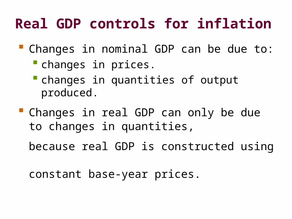
Real GDP controls for inflation
Changes in nominal GDP can be due to: changes in prices. changes in quantities of output produced.
Changes in real GDP can only be due to changes in quantities,
because real GDP is constructed using constant base-year prices.
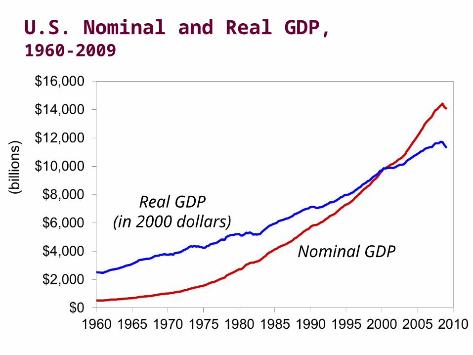
U.S. Nominal and Real GDP,1960-2009
Nominal GDP
Real GDP(in 2000 dollars)
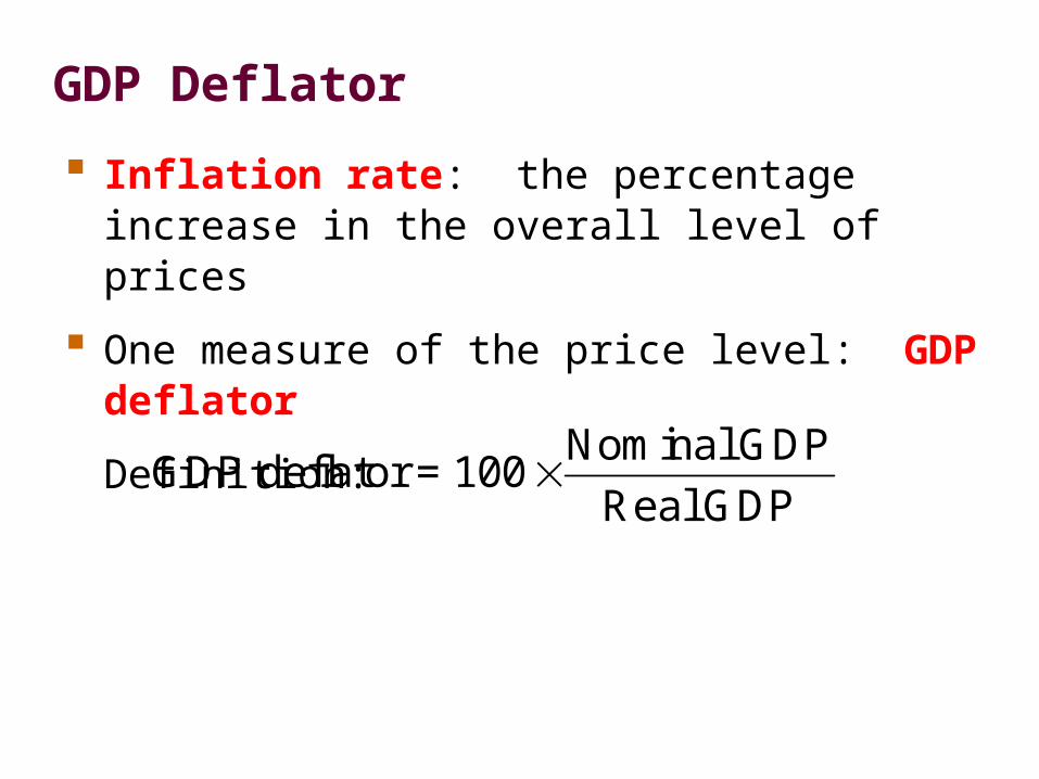
GDP Deflator
Inflation rate: the percentage increase in the overall level of prices
One measure of the price level: GDP deflator
Definition:
Nominal GDP
GDP deflator = 100Real GDP
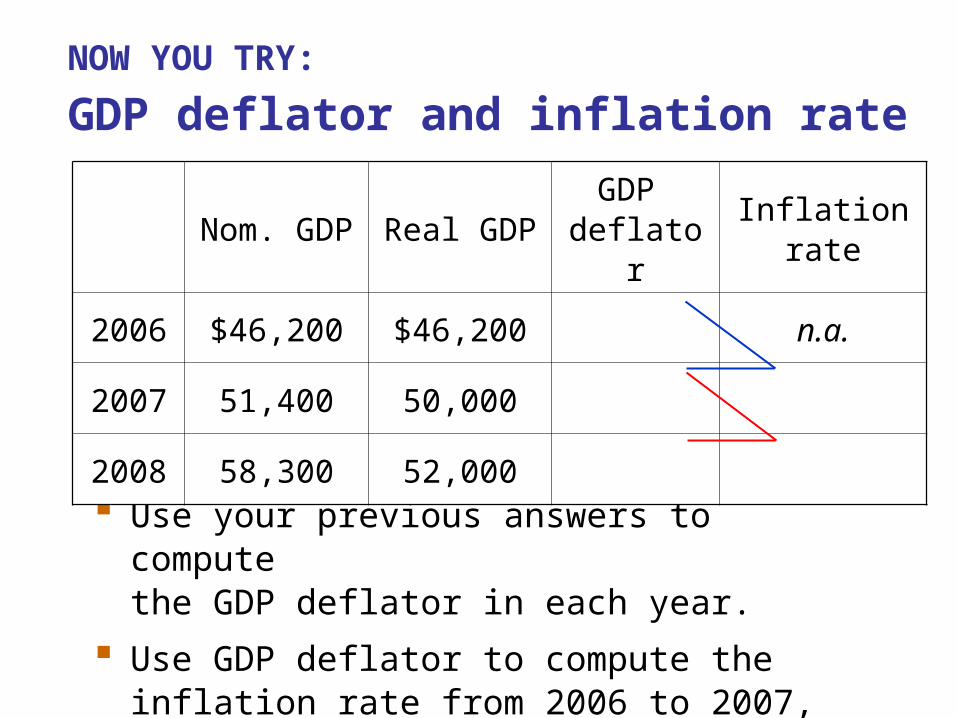
NOW YOU TRY:
GDP deflator and inflation rate
Use your previous answers to compute the GDP deflator in each year.
Use GDP deflator to compute the inflation rate from 2006 to 2007, and from 2007 to 2008.
Nom. GDP Real GDPGDP
deflatorInflation
rate
2006 $46,200 $46,200 n.a.
2007 51,400 50,000
2008 58,300 52,000
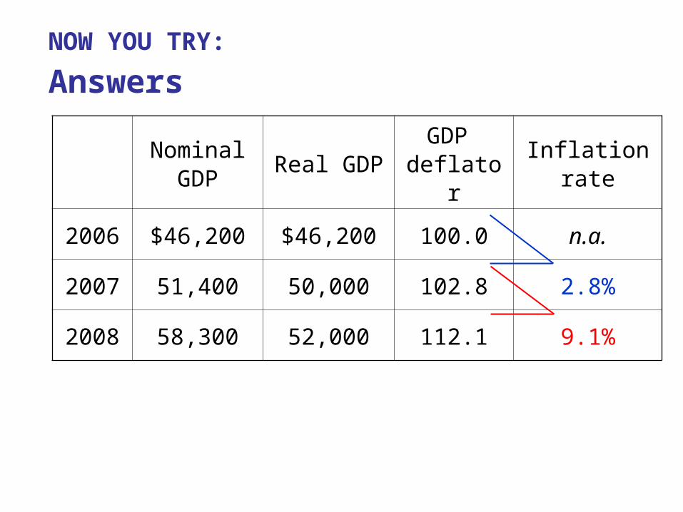
NOW YOU TRY:
Answers
Nominal GDP
Real GDPGDP
deflatorInflation
rate
2006 $46,200 $46,200 100.0 n.a.
2007 51,400 50,000 102.8 2.8%
2008 58,300 52,000 112.1 9.1%
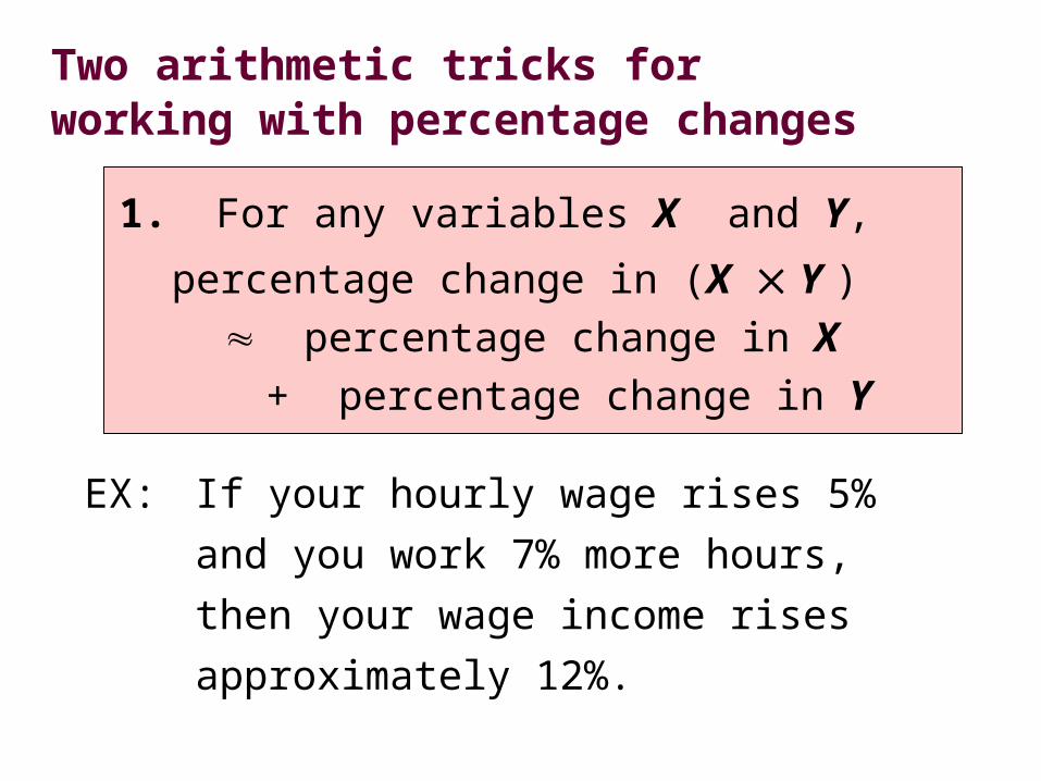
Two arithmetic tricks for working with percentage changes
EX: If your hourly wage rises 5%
and you work 7% more hours,
then your wage income rises
approximately 12%.
1. For any variables X and Y,
percentage change in (X Y )
percentage change in X
+ percentage change in Y
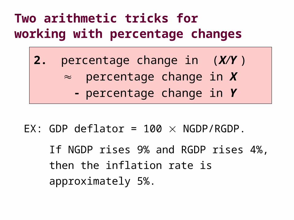
Two arithmetic tricks for working with percentage changes
EX: GDP deflator = 100 NGDP/RGDP.
If NGDP rises 9% and RGDP rises 4%,
then the inflation rate is approximately 5%.
2. percentage change in (X/Y )
percentage change in X
percentage change in Y
Chain-Weighted Real GDP
Over time, relative prices change, so the base year should be updated periodically.
In essence, chain-weighted real GDP updates the base year every year, so it is more accurate than constant-price GDP.
Your textbook usually uses constant-price real GDP, because:
the two measures are highly correlated.
constant-price real GDP is easier to compute.
Consumer Price Index (CPI)
A measure of the overall level of prices
Published by the Bureau of Labor Statistics (BLS)
Uses:
tracks changes in the typical household’s cost of living
adjusts many contracts for inflation (“COLAs”)
allows comparisons of dollar amounts over time

How the BLS constructs the CPI
1. Survey consumers to determine composition of the typical consumer’s “basket” of goods
2. Every month, collect data on prices of all items in the basket; compute cost of basket
3. CPI in any month equals
Cost of basket in that month
Cost of basket in base period100
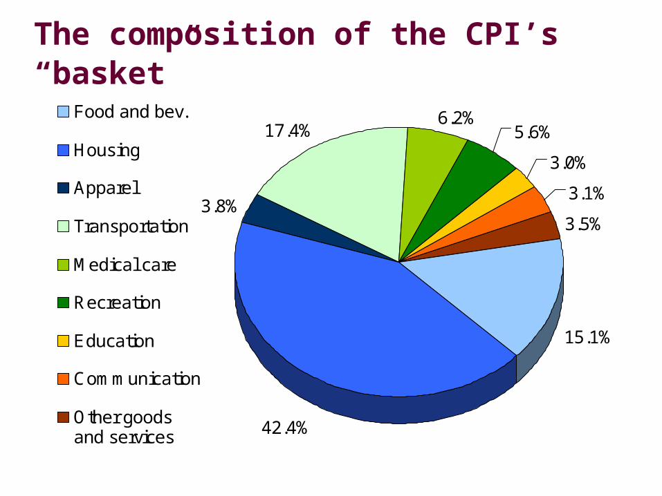
The composition of the CPI’s “basket”
15.1%
42.4%
3.8%
17.4%6.2%
5.6%
3.0%
3.1%
3.5%
Food and bev.
Housing
Apparel
Transportation
Medical care
Recreation
Education
Communication
Other goodsand services
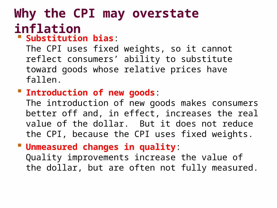
Why the CPI may overstate inflation Substitution bias:
The CPI uses fixed weights, so it cannot reflect consumers’ ability to substitute toward goods whose relative prices have fallen.
Introduction of new goods: The introduction of new goods makes consumers better off and, in effect, increases the real value of the dollar. But it does not reduce the CPI, because the CPI uses fixed weights.
Unmeasured changes in quality: Quality improvements increase the value of the dollar, but are often not fully measured.
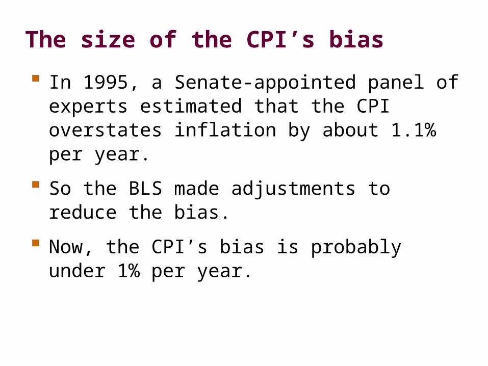
The size of the CPI’s bias
In 1995, a Senate-appointed panel of experts estimated that the CPI overstates inflation by about 1.1% per year.
So the BLS made adjustments to reduce the bias.
Now, the CPI’s bias is probably under 1% per year.
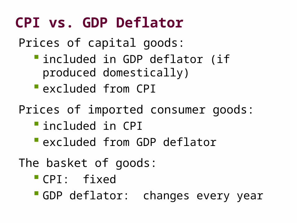
CPI vs. GDP DeflatorPrices of capital goods:
included in GDP deflator (if produced domestically)
excluded from CPI
Prices of imported consumer goods: included in CPI excluded from GDP deflator
The basket of goods: CPI: fixed GDP deflator: changes every year

The PCE deflator
Another measure of the price level: Personal Consumption Deflator, the ratio of nominal to real consumer spending
How the PCE is like the CPI:- only includes consumer spending- includes imported consumer goods
How the PCE is like the GDP deflator:- the “basket” changes over time
The Federal Reserve prefers PCE.

The GDP deflator, CPI, and PCE deflator
CPI
GDP deflator
PCE deflator
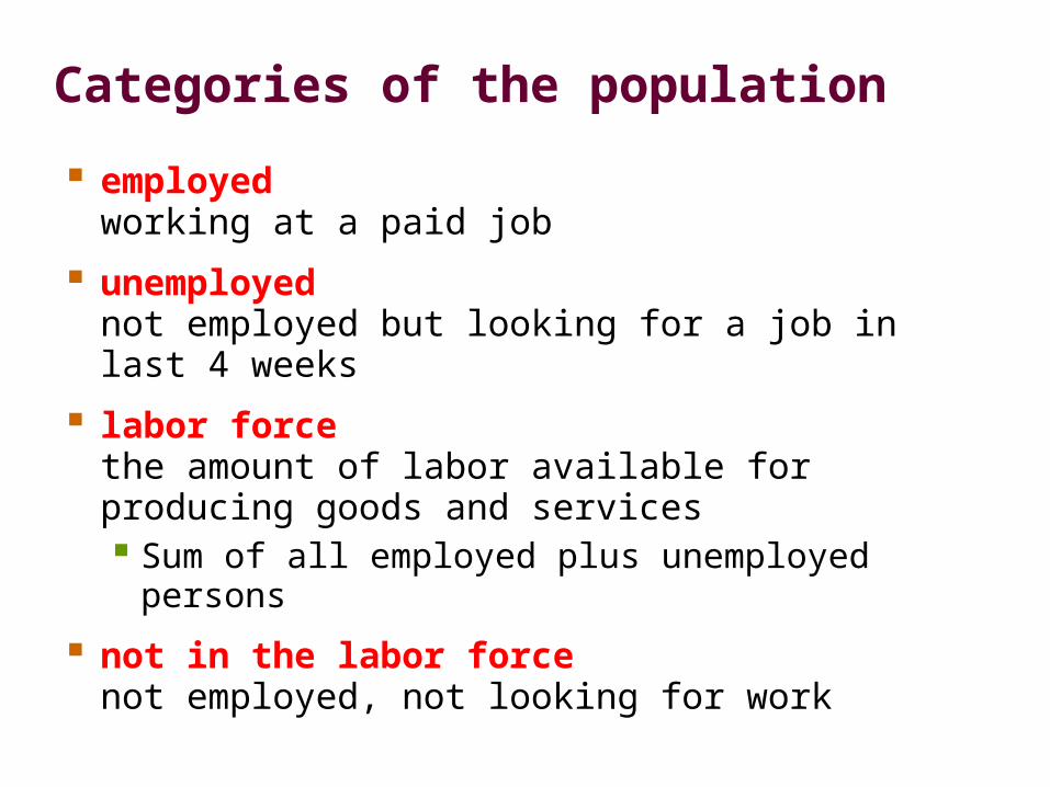
Categories of the population
employed working at a paid job
unemployed not employed but looking for a job in last 4 weeks
labor force the amount of labor available for producing goods and services Sum of all employed plus unemployed persons
not in the labor force not employed, not looking for work
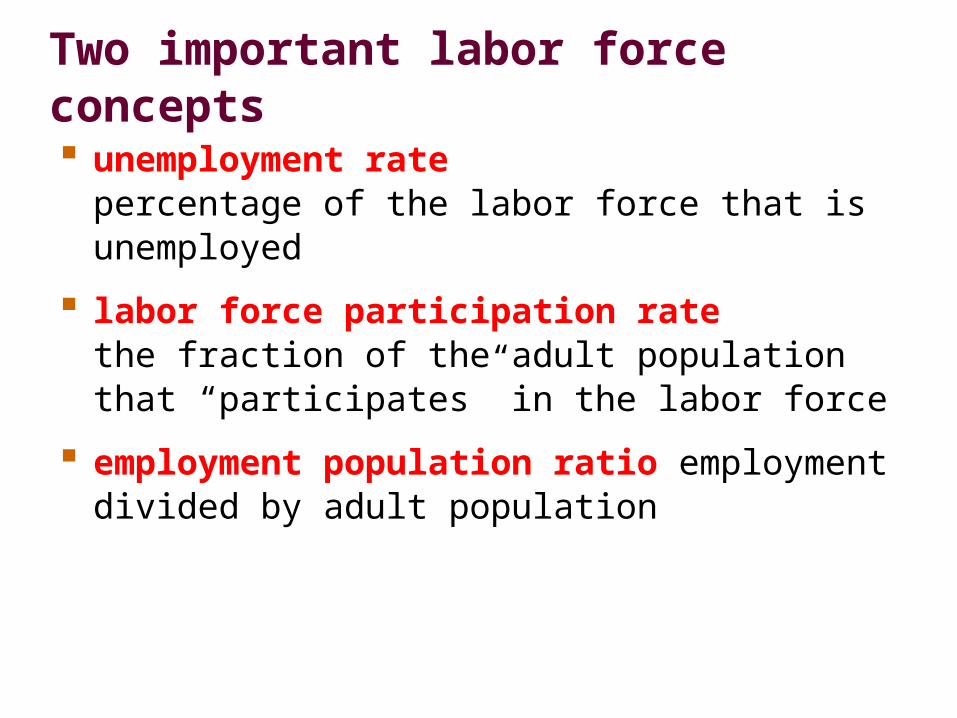
Two important labor force concepts unemployment rate
percentage of the labor force that is unemployed
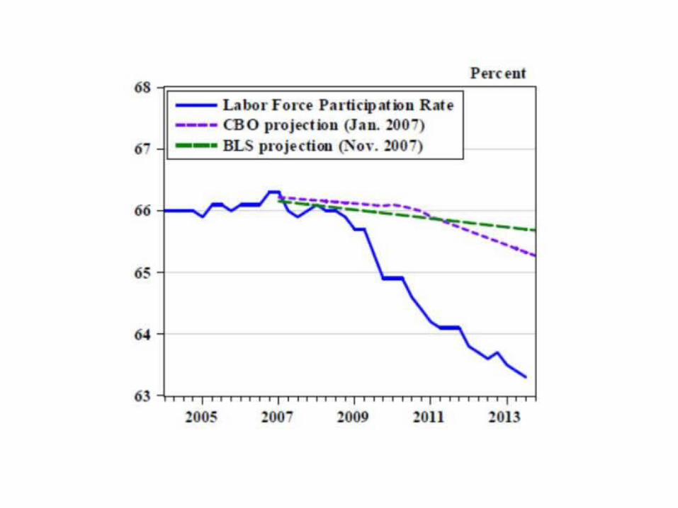
labor force participation rate the fraction of the adult population that “participates” in the labor force
employment population ratio employment divided by adult population
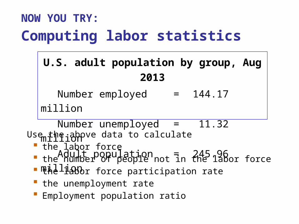
NOW YOU TRY:
Computing labor statistics
U.S. adult population by group, Aug 2013
Number employed = 144.17 million
Number unemployed = 11.32 million
Adult population = 245.96 million
Use the above data to calculate the labor force the number of people not in the labor force the labor force participation rate the unemployment rate Employment population ratio
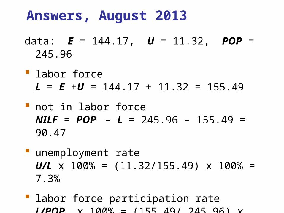
Answers, August 2013
data: E = 144.17, U = 11.32, POP = 245.96
labor forceL = E +U = 144.17 + 11.32 = 155.49
not in labor forceNILF = POP – L = 245.96 – 155.49 = 90.47
unemployment rateU/L x 100% = (11.32/155.49) x 100% = 7.3%
labor force participation rateL/POP x 100% = (155.49/ 245.96) x 100% = 63.22%
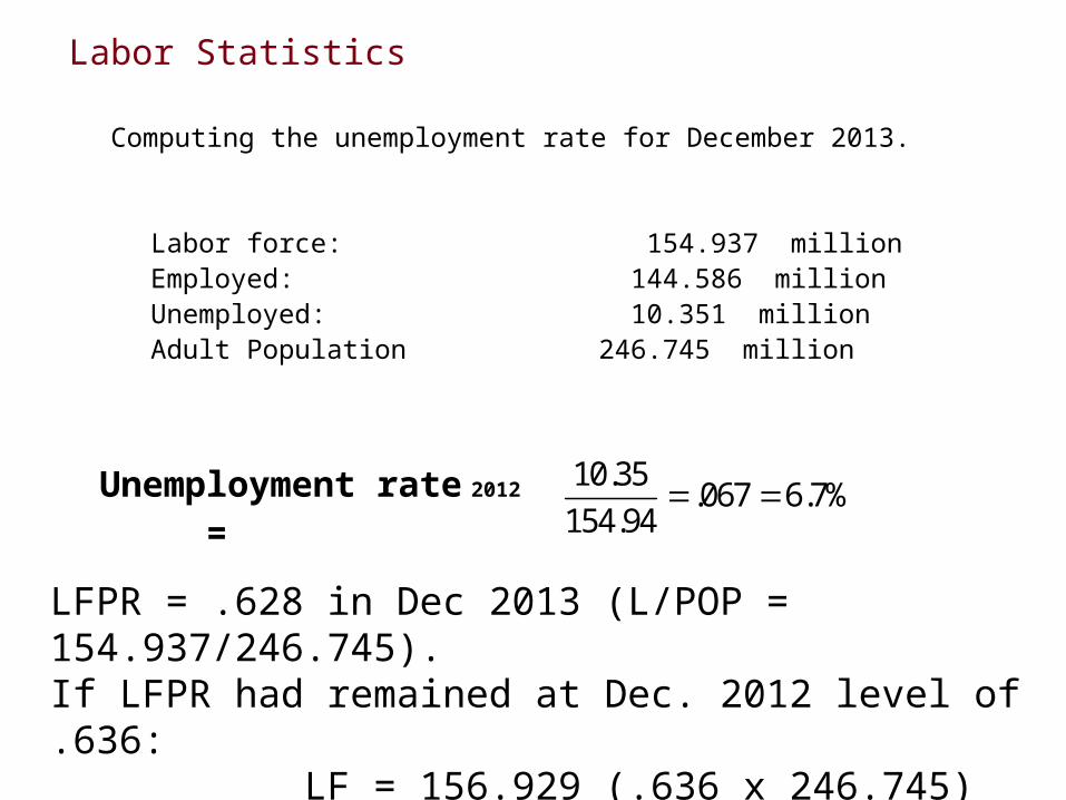
Labor Statistics
Computing the unemployment rate for December 2013.
Labor force: 154.937 million Employed: 144.586 million Unemployed: 10.351 million Adult Population 246.745 million
Unemployment rate 2012 =
10.35.067 6.7%
154.94
LFPR = .628 in Dec 2013 (L/POP = 154.937/246.745).If LFPR had remained at Dec. 2012 level of .636: LF = 156.929 (.636 x 246.745) and U/L = 12.34/156.929 = 7.8%
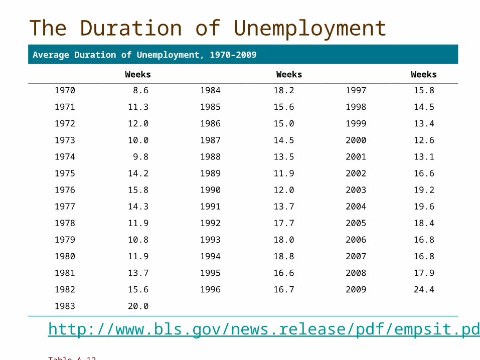
Average Duration of Unemployment, 1970–2009
Weeks Weeks Weeks
1970 8.6 1984 18.2 1997 15.8
1971 11.3 1985 15.6 1998 14.5
1972 12.0 1986 15.0 1999 13.4
1973 10.0 1987 14.5 2000 12.6
1974 9.8 1988 13.5 2001 13.1
1975 14.2 1989 11.9 2002 16.6
1976 15.8 1990 12.0 2003 19.2
1977 14.3 1991 13.7 2004 19.6
1978 11.9 1992 17.7 2005 18.4
1979 10.8 1993 18.0 2006 16.8
1980 11.9 1994 18.8 2007 16.8
1981 13.7 1995 16.6 2008 17.9
1982 15.6 1996 16.7 2009 24.4
1983 20.0
The Duration of Unemployment
http://www.bls.gov/news.release/pdf/empsit.pdf
Table A-12
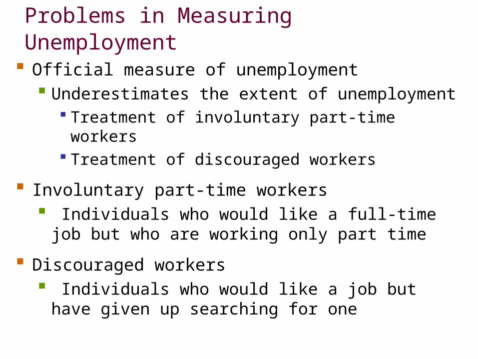
Problems in Measuring Unemployment
Official measure of unemployment Underestimates the extent of unemployment
Treatment of involuntary part-time workers Treatment of discouraged workers
Involuntary part-time workers Individuals who would like a full-time job but who
are working only part time
Discouraged workers Individuals who would like a job but have given up
searching for one
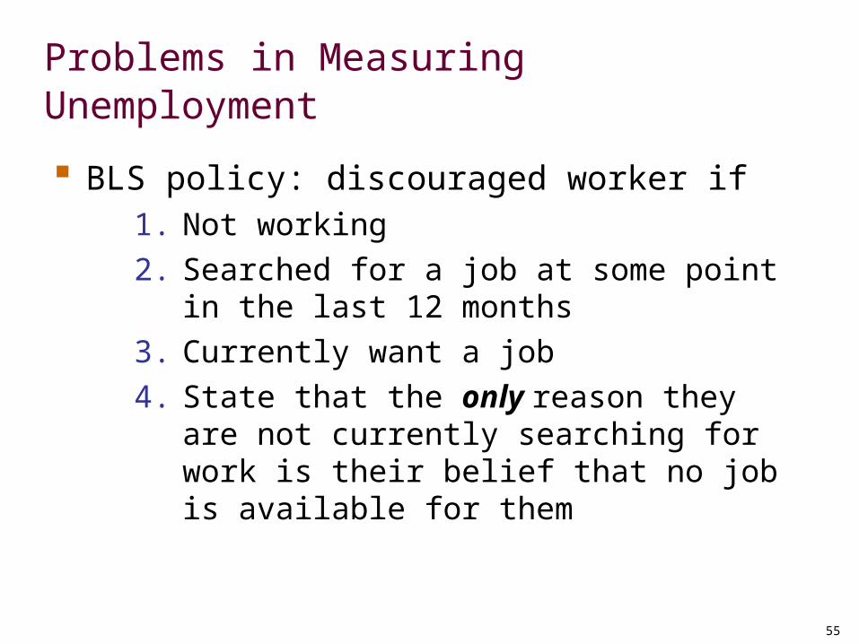
Problems in Measuring Unemployment
BLS policy: discouraged worker if 1. Not working
2. Searched for a job at some point in the last 12 months
3. Currently want a job
4. State that the only reason they are not currently searching for work is their belief that no job is available for them
55
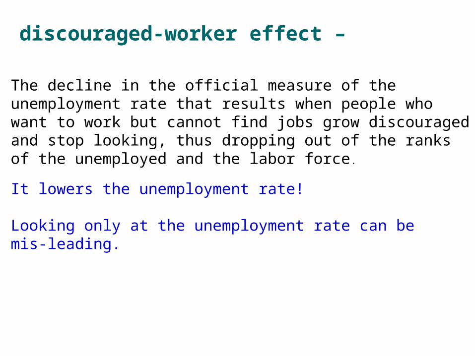
discouraged-worker effect –
The decline in the official measure of the unemployment rate that results when people who want to work but cannot find jobs grow discouraged and stop looking, thus dropping out of the ranks of the unemployed and the labor force .
It lowers the unemployment rate!
Looking only at the unemployment rate can be mis-leading.
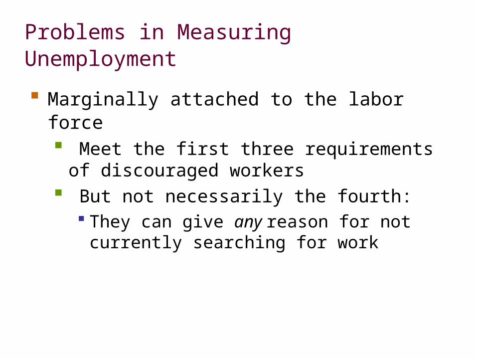
Problems in Measuring Unemployment
Marginally attached to the labor force Meet the first three requirements of
discouraged workers But not necessarily the fourth:
They can give any reason for not currently searching for work
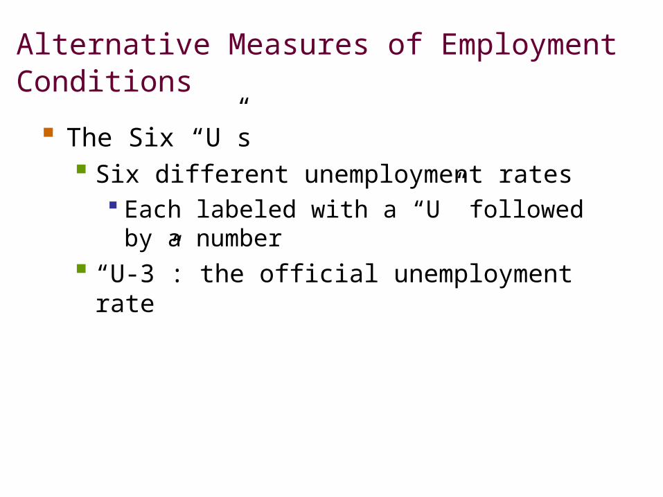
Alternative Measures of Employment Conditions
The Six “U”s Six different unemployment rates
Each labeled with a “U” followed by a number “U-3”: the official unemployment rate
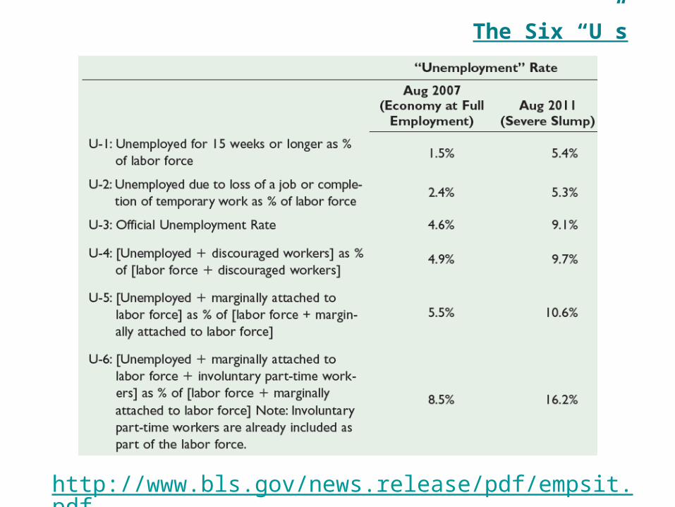
The Six “U”s
http://www.bls.gov/news.release/pdf/empsit.pdf Table A-15

Alternative Measures of Employment Conditions
The employment-population ratio Total employment (from the household survey)
divided by the total population over age 16 Tracks the fraction of the adult population that
is working not affected by job-searching behavior
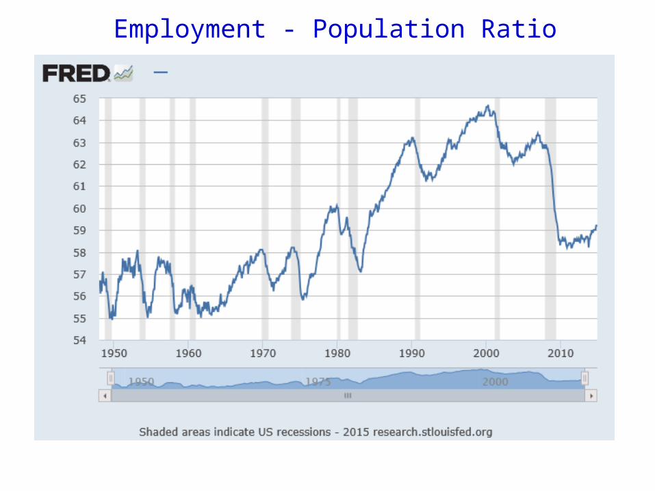
Employment - Population Ratio
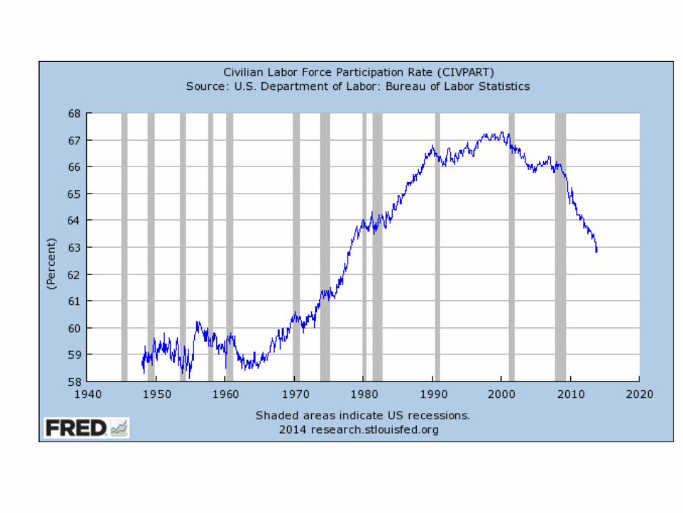
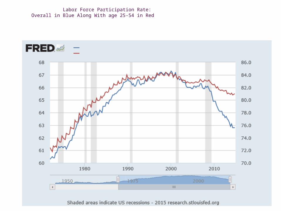
Labor Force Participation Rate: Overall in Blue Along With age 25-54 in Red