Chapter 2 Consumption Tax - Hitotsubashi University

Lectures on Public Finance Part2_Chap2, 2016 version P.1 of 55 Last updated 18/10/2016

Chapter 2 Consumption Tax

2.1 Consumption Tax in Practice1 One often hears that a consumption tax would be unjust, since the rich consume less (as a proportion of income) than the poor. We will see that by using judiciously the equivalences recalled above, one may conceive a consumption tax that is as progressive as one likes. The frequent assimilation of the consumption tax to a renunciation to progressivity is a confusion that partly results from the fact that many proponents of the consumption tax indeed favor a proportional income tax: the flat tax. A proportional (income or consumption) tax would have obvious administrative advantages. First, it would simplify (marginally) the tax returns2. It would also eliminate one of the anomalies of progressive taxes: with such schedules a taxpayer pays more tax when his income varies over time than when it is constant. Finally, it would make pay-as-you-earn withholding systems much simpler when the taxpayer has several sources of income. Despite these advantages most voters estimate that taxes should be progressive. Thus the tax acts proposed usually comprise a personal exemption that takes the poorer families off the tax rolls; this clearly detracts from the advantage of strict proportionality3. There are many ways to make a consumption tax progressive. In general, a consumption tax is the combination of a corporate tax and a personal tax4. The corporate tax often is a proportional tax on noninvested value added. Since investment is deducted from the taxable basis, this amounts to allowing for immediate depreciation of all capital investment, which is a simple if radical way of equating fiscal depreciation and economic depreciation. It also restores the neutrality toward all forms of investment, which is a radical change on current income taxes. In the best-known blueprint, due to Hall and Rabuschka (1995), wages paid by firms are deducted from noninvested value added before computing the corporate tax; the personal tax is a tax on all wage income received by families. Changing the schedule of this personal wage tax allows the government to achieve any degree of progressivity. Opponents of the consumption tax justly remark that such a wage tax would exempt people who have had 1 This section draws from Salanié (2003, Chap. 9, pp.190-2). 2 Several presidential candidates in the United States have taken to waving a postcard as the promise of a much

simpler tax return. 3 This type of tax schedule was already the favorite of classical authors, from Smith to Mill. 4 Some proponents of the consumption tax seek to abolish all personal taxes by relying on a tax on (noninvested)

value added, which is the same as a consumption tax as we know. The disadvantage of this method is that it makes it hard to make the tax progressive.


the good fortune of a large bequest and live off it without working. Most people find this immoral, so the wage tax should be complemented with a progressive tax on bequests. Another possibility (the Unlimited Savings Allowance or USA Tax; see Seidman (1997)) consists in taxing families in a progressive manner on the difference between the money flows they receive (whether it is labor income or capital income) and their savings, since this difference by definition equals their consumption. The USA Tax was inspired by the writings of Irving Fisher; it supposes that families keep proper accounts of their money flows (in and out) that are not linked to consumption. To make it equivalent to a tax on wages and bequests received, the USA Tax should also tax the bequests left by taxpayers. Proponents of the consumption tax predict a large positive effect on savings and, since the economy is assumed to have too little capital, on welfare. There have been many quantitative studies on this topic. They usually do obtain a positive effect on welfare, but with very variable figures. One of the most serious problems of such a reform arises when moving from an income tax to a consumption tax. The unfortunate taxpayers who have saved while paying the income tax, hoping to live off the income from their savings without paying any more tax, now have to pay the consumption tax. This could represent a large welfare loss for them. The proposed reforms thus all contain more or less satisfactory clauses to account for this so-called old wealth problem (See Chapter 6 for related topics).

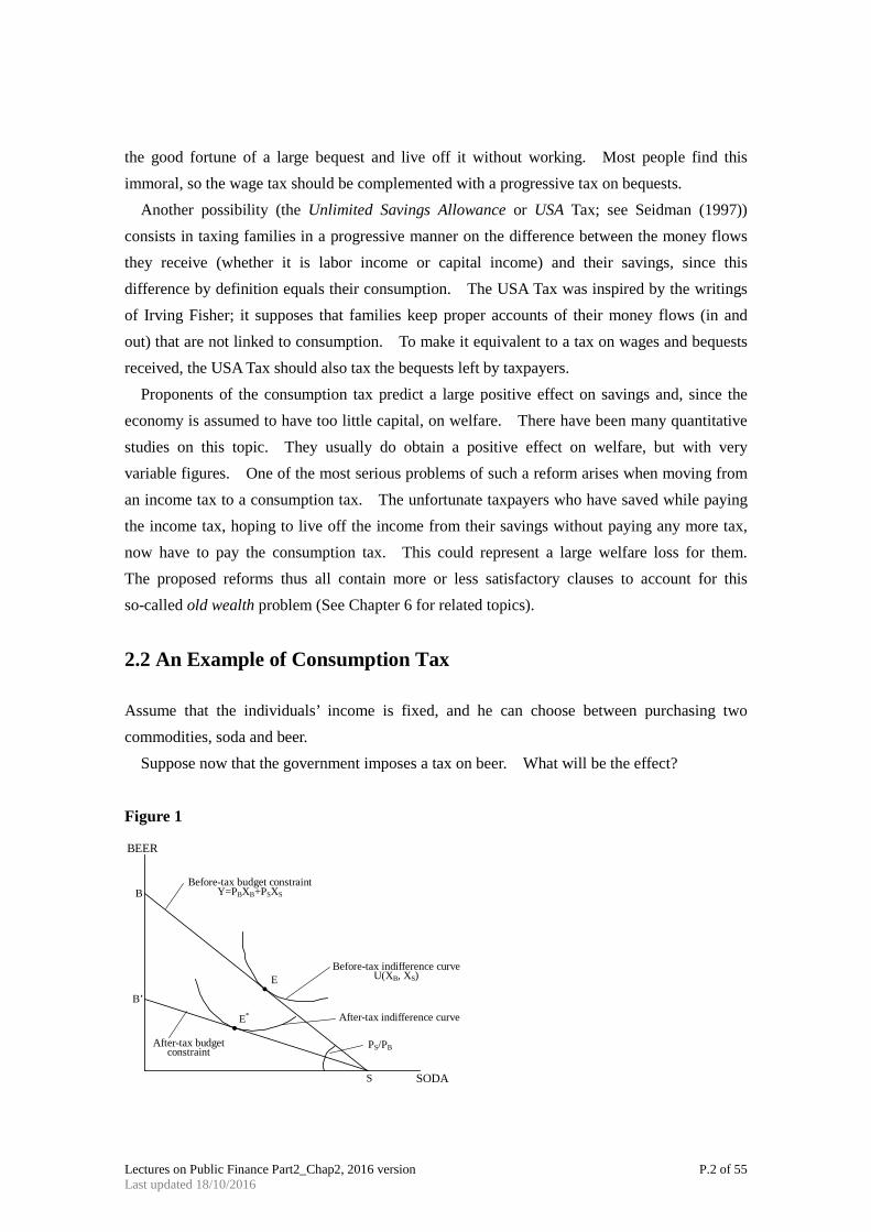
2.2 An Example of Consumption Tax Assume that the individuals’ income is fixed, and he can choose between purchasing two commodities, soda and beer. Suppose now that the government imposes a tax on beer. What will be the effect? Figure 1 BEER

SODA

•

• PS/PB

S

B’

B

E

E*

After-tax budget constraint

Before-tax budget constraint Y=PBXB+PSXS

After-tax indifference curve

Before-tax indifference curve U(XB, XS)


Initially, the individual allocated his income by choosing point E on his budget constraint. This is the point of tangency between the budget constraint and the before-tax indifference curve. After the imposition of the tax, there is a new equilibrium, at point E*. We can decompose the effects of the tax into two parts. The income effect reduces the demand for beer. In addition however, the tax has increased the price of beer relative to the price of soda, so the substitution effect will discourage the purchase of beer. Now, both the income and the substitution effects reinforce each other: they both lead to a reduction in the demand for beer. But the distortionary effect of the tax is only associated with the substitution effect. To see this, we contrast the effect of the beer tax with that of a lump sum tax. A lump sum tax represents a reduction in the amount of income the individual can spend on either commodity. The relative price of the two commodities remains unchanged. If we measure the tax in terms of beer, the tax revenue is represented by the vertical distance between the before-tax and after-tax budget constraints. In Figure 2, we can compare the revenues raised by a beer tax with those raised by a lump sum tax, with equal effect on the level of utility. Figure 2

It is clear from the figure that the lump sum tax raises more revenue (and leads to a higher level of consumption of beer) than does the beer tax. The difference between the two is a measure of the inefficiency resulting from the tax --- the deadweight loss associated with the tax. If it is very difficult to substitute soda for beer, i.e. if the indifference curves are very curved --- the distortion associated with the tax is very small. The magnitude of the distortion can vary from commodity to commodity.

BEER

SODA

•

•

E**

E* Budget constraint after beer tax

Before-tax budget constraint

After-tax indifference curve

•

•

Deadweight Loss

Lump sum tax revenue

Beer tax revenue


2.3 Equivalences between Taxes5 We focus here on ideal taxes that are both proportional and comprehensive (with no special provisions). Then a first equivalence links a uniform tax on incomes of all factors and a uniform VAT on all goods. A uniform VAT indeed has exactly the same economic effects as a uniform factor tax of the same rate. This result must be slightly modified in the many countries whose VAT allows firms to deduct investment from value added (just as they do with intermediate consumptions). Then VAT bears on noninvested value added, and it is equivalent to a tax on that part of income that is not invested, or again to a consumption tax.

In a world where financial markets are perfect, we can write the intertemporal budget constraint of a consumer-worker who lives T periods, receives a bequest 1H and leaves a bequest TS as

11

11

1 )1()1()1(H

rLw

rS

rC T

tt

ttT

TT

tt

t ++

=+

++ ∑∑

=−

=−

This equality shows that if there are no bequests, then a consumption tax is exactly equivalent to a wage tax – which is not an income tax since it does not tax income from savings. More generally, a tax on both consumption and bequests left is equivalent to a tax on both wages and bequests received. Recall that these equivalences only hold for uniform, comprehensive, and proportional taxes, whereas actual taxes are neither of these three. Still, they throw some light on the debate on the consumption tax.

The Comprehensive Income Tax The income tax as we know it is a rather hybrid construction: it taxes income from various forms of savings in a very unequal way and relies on a concept of income that satisfies few economists. Since the work of Haig and Simons in the 1930s, economists indeed have leaned toward a definition of comprehensive income as the total amount that can be allocated to consumption or savings in a given period. To understand this, consider the equation that sums up the changes in an agent’s wealth. During a period t, the agent receives wage income, consumes, and gets a rate of return tr on its beginning-of-period wealth tA . His end-of-period wealth 1+tA then is

tttttt CLwrAA −++=+ )1(1

5 This and the next sections draws from Salanié (2003, Chap. 9, pp.187-90).


This equality allows us to define comprehensive income tY as

tttttttt ArLwAACY +=−+= + )( 1

Thus comprehensive income is the sum of the agent’s consumption and the increase in his wealth. To put it differently, it is the amount the agent may consume without reducing his wealth (for tt AA =+1 , we get tt YC = ). The equality above shows that comprehensive income can also be defined as the sum of wage income and return on wealth tt Ar . If the

return on wealth is entirely accounted for by interest and dividends, then it is included in the usual definition of income and thus comprehensive income coincides with national accounts income. On the other hand, national accounts income only accounts for capital gains (the appreciation of stocks, housing, ets.) when they are realized, that is, just before the underlying asset is sold. Comprehensive income accounts for these capital gains even when they are latent, that is, before the agent even considers selling the asset. Take a bullish period on the stockmarket; then consumers who own shares will probably boost their consumption since they perceive a higher wealth. Comprehensive income explains this, while national accounts income does not even register the latent capital gains. Several economists start from this more satisfactory definition of income to argue that the income tax should be a comprehensive income tax. This amounts to saying that the income tax should also tax latent capital gains. This is not a trivial change ,as many families own stocks and even more own their house. Beyond the argument above, the proponents of a comprehensive income tax note that the current income tax creates a lock-in effect: since it only taxes capital gains when they are realized (and not at all when the owner of the asset dies), it provides incentives for owners to keep the asset for longer than they would in a world without taxes. These economists also insist on the importance of accounting for inflation properly. Recall that comprehensive income is the sum of consumption and the real increase in wealth, so that a comprehensive income tax would only tax real income from savings. On the other hand, the current income tax taxes the nominal income from savings. In inflationary periods it also taxes pseudo-income that contributes nothing to consumption or increases in wealth. Thus a 50 percent tax rate on income from savings in fact confiscates the whole real return from savings when inflation is 2 percent and the nominal interest rate is 4 percent. The creation of a comprehensive income tax would imply a notable extension of the taxable basis, since this would include latent capital gains and all the income from various sources of savings that are currently tax-favored6. Advocates of a consumption tax go to the polar opposite, since they would exempt all income from savings, whether it consists of interests,

6 The most spectacular exemption in many – but not all – current income tax systems concerns fictitious rents, that

is, the rental value of an owner-occupied house. These rents are implicitly received by the owner and in fact constitute income from the savings materialized in the house.


dividends, or capital gains (latent or realized).

Annual versus Lifetime Equity Events that influence a person’s economic position for only a very short time do not provide an adequate basis for determining ability to pay. Some have argued that ideally tax liabilities should be related to lifetime income. Proponents of consumption taxation point out that an annual income tax leads to tax burdens that can differ quite substantially even for people who have the same lifetime wealth. Borrowing an example from Rosen (1999), consider Mr. Grasshopper and Ms. Ant, both of whom live for two periods. In the present, they have identical fixed labor incomes of Y0 and in the future, they both have labor incomes of zero (for convenience). Grasshopper chooses to consume heavily early in life because he is not very concerned about his retirement years. Ant chooses to consume most of her wealth later in life, because she wants a affluent retirement. Define Ant’s present consumption in the presence of a proportional income tax as Co

A and Grasshopper’s as Co

G. By assumption, CoG > Co

A. Ant’s future income before tax is the interest she earns on her savings: )( 00

ACYr − . Grasshopper’s future income before tax is )( 00

GCYr − . If the proportional income tax rate is t, in the present Ant and Grasshopper have identical tax liabilities of 0tY . However, in the future, Ant’s tax liability is )( 00

ACYtr − . Because of CoG

> CoA, Ant’s future tax liability is higher. Solely because Ant has a greater taste for saving than

Grasshopper, her lifetime tax burden is greater than Grasshopper’s. In contrast, under a proportional consumption tax, lifetime tax burdens are independent of tastes for saving, other things being the same7. To prove this, all we need to do is write down the equation for each taxpayer’s budget constraint. Because all of Ant’s noncapital income ( oI ) comes in present, its present value is simply oI . Now, the present value of lifetime

consumption must equal the present value of lifetime income. Hence, Ant’s consumption pattern must satisfy the relation

rc

cIAoA

oo ++=

1 (1)

Similarly, Grasshopper is constrained by

7 However, when marginal tax rates depend on the level of consumption, this may not be the case.


rc

cIG

Goo ++=

11 (2)

Equations (1) and (2) say simply that the lifetime value of income must equal the lifetime value of consumption. If the proportional consumption tax rate is ct , Ant’s tax liability in the first period is A

occt ; her tax liability in the second period is A

cct 1 ; and the present value of her lifetime consumption tax liability, A

cR , is

rct

ctRA

cAoc

Ac +

+=1

1 (3)

Similarly, Grasshopper’s lifetime tax liability is

rct

ctRG

cGoc

Gc +

+=1

1 (4)

By comparing Equations (3) and (1), we see that Ant’s lifetime tax liability is equal to oc It .

Similar comparison of Equations (2) and (4) indicates that Grasshopper’s lifetime tax liability is also oc It . We conclude that under a proportional consumption tax, two people with

identical lifetime incomes always pay identical lifetime taxes (where lifetime is interpreted in the present value sense). This stands in stark contrast to a proportional income tax, where the pattern of lifetime consumption influences lifetime tax burdens. A related argument in favor of the consumption tax centers on the fact that income tends to fluctuate more than consumption. In years when income is unusually low, individuals may draw on their savings or borrow to smooth out fluctuations in their consumption levels. Annual consumption is likely to be a better reflection of lifetime circumstances than is annual income. Opponents of consumption taxation would question whether a lifetime point of view is really appropriate. There is too much uncertainty in both the political and economic environments for a lifetime perspective to be very realistic. Moreover, the consumption smoothing described in the lifetime arguments requires that individuals be able to save and borrow freely at the going rate of interest. Given that individuals often face constraints on the amounts they can borrow, it is not clear how relevant the lifetime arguments are. Although a considerable body of empirical work suggests the life-cycle model is a good representation for most households (see King (1993)), this arguments still deserves some consideration.


2.4 The General Model8

Now consider the general equilibrium of a simple production economy. The economy consists of I consumer-workers with utility functions ),( iii LXU , where iX represents consumptions of the n goods and iL is the supply of labor. For a start, we assume that production has

constant returns of the simplest variety: each good is produced from labor alone. Production of a unit of good j requires

ja units of labor so that the production price can only be

wap jj = in equilibrium. We choose to normalize 1=w ; moreover we choose the units of goods so that each ja equals one, so that all production prices satisfy 1=jp .

Since this is a general equilibrium model, we must specify how the government intervenes in the economy. The government may want to pay civil servants, finance the production of public goods, or purchase private goods. To simplify, we assume here that it just buys T units of labor. Since the wage is normalized to one, the government must collect revenue T. We consider the following taxes:

・ linear taxes on goods, which raise consumer prices to )1( jt+

・ a linear tax on wages, so that the after-tax wage is )1( τ− .

The budget constraint of consumer i, who only owns his labor force, then is

i

n

jijj LXt )1()1(

1

τ−=+∑=

(5)

It is easy to see that in this setting (with no nonlabor income, and no bequests), the tax on wages is equivalent to a uniform tax on goods. Indeed define

ττ−

+=

1' jj

tt (6)

Since )1)(1(1 ' τ−+=+ jj tt , we can rewrite the budget constraint of consumer i as

i

n

jijj LXt∑

=

=+1

' )1( (7)

8 Section 2.4 and 2.5 draw from Salanié (2003, pp.64-73).


The tax system )),(( τjt then is equivalent for all consumers to the tax system )0),(( 'jt , which

does not tax wages. Replacing the former with the latter leaves consumer choices unchanged. Moreover the government collects from consumer i with the former tax system

i

n

jijj LXt∑

=

+1

τ (8)

But using the consumer i’s budget constraint

∑=

+=n

jijji XtL

1

' )1( (9)

this tax revenue can also be written

∑∑==

=++n

jijj

n

jijjj XtXtt

1

'

1

' ))1(( τ (10)

which is exactly what the government collects from consumer i in the latter tax system. Thus a tax on wages is absolutely equivalent to a uniform tax on goods.

As a consequence only n of the )1( +n rates )),(( τjt are determined at the optimum,

whatever that is. We may, for instance, fix arbitrarily the rate of the tax on wages. This hardly matters, since we focus here on how taxes are differentiated across goods, and '

jt

notation, which fixes 0=τ . We will work on the indirect utility of consumers, which can be written )(qVi , where

'1 tq += is the vector of consumption prices:

),(max)(),(

iiiLX

i LXUqVii

= under ii LXq =⋅ (11)

We are in a second-best situation, since we do not allow for the lump-sum transfers that would implement any Pareto optimum. To model the redistributive objectives of government, we assume that it maximizes a Bergson-Samuelson functional

))(,),(()( 1 qVqVWq I=W (12)


To fulfill its needs in the most efficient way, the government must maximize )(qW in q under its budget constraint (remember that '1 tq += , so choosing the tax rates is equivalent to

choosing the consumption prices):

TqXq ij

I

i

n

jj =−∑∑

= =

)()1(1 1

(13)

Where the )(qX i

j are the demands of the various consumers9.

Let λ denote the Lagrange multiplier of the budget constraint of government. We have, by differentiating in kq ,

∑ ∑∑= ==

∂

∂+−=

∂∂

∂∂

I

i

n

j k

ijjik

k

iI

i i qX

tXqV

V1 1

'

1

W λ (14)

By Roy’s identity,

ikik

i XqV α−=∂∂ (15)

where iα is the marginal utility of income of i . We define

ii

i Vαβ

∂∂

=W

(16)

This new parameter weights the marginal utility of income of consumer i by his weight in the social welfare function; iβ is called the social marginal utility of income of i , since it is the

increase in the value of the Bergson-Samuelson functional when i is given one more unit of income.

We have, by substituting these definitions,

9 We should note here that the indirect utilities )(qVi

are quasi-convex, so that even though W is concave, the

program we shall solve may not be concave. Diamond-Mirrlees (1971b) prove that the calculations that follow can nevertheless be rigourously justified.


∑ ∑∑= ==

∂

∂+=

I

i

n

j k

ijjik

I

iiki q

XtXX

1 1

'

1

λβ (17)

We will now use Slutsky’s equation

i

ijik

ijk

k

ij

RX

XSqX

∂

∂−=

∂

∂ (18)

where we defined

iUk

ijijk q

XS

∂

∂= (19)

We get, by rearranging,

∑∑∑∑∑===

=

==∂

∂+−

∑=

n

j i

ijj

I

iik

I

iik

ikiIi

I

i

ijk

n

jj R

XtXX

XSt

1

'

11

1

11

'λβ (20)

which contains the new parameter

∑=

∂

∂+=

n

j i

ijj

ii R

Xtb

1

'λβ (21)

The first term of ib is the social marginal utility of income of i , divided by λ , which is the

cost of budget resources for the government; the second term is the increase in tax revenue collected on i when his income increases by one unit. The parameter ib thus measures

what is called the net social marginal utility of income of consumer i . It accounts not only for the direct term λβ /i of social utility (measured in monetary units) but also for the fact that the increase in taxes paid by i allows to reduce tax rates. Of course, ib is endogenous, just like iβ .

Let us denote the aggregate demand for good k by ikIik XX 1=∑= . Rearranging and using

the symmetry of the Slutsky matrix, we finally get


−−= ∑∑∑

=== k

ikI

iik

I

i

ikj

n

jj X

XbXSt

111

' 1 (22)

By definition,

11

=∑=

I

i k

ikXX (23)

Denote b as the average of the s'ib and define the empirical covariance (across consumers) as

=

k

ikik X

IXbb ,covθ (24)

We can now write

kk

ikj

Iij

nj bb

XSt

θ−−=∑∑

− == 11'

1 (25)

which is Ramsey’s formula with several consumers, first obtained in this form by Diamond (1975).

The left-hand side of this equation is called the discouragement index of good k . Let indeed the '

jt be small (which must hold if the government collects a low tax revenue T ). Then the tax '

jt on good j reduces the consumption of good k by consumer i by ikjj St ' at

a fixed utility level. The left-hand side is, to a first-order approximation, minus the percentage of decrease of the consumption of good k summed across consumers. Thus it can be interpreted as the relative reduction in the compensated demand for good k induced by the tax system.

As for the right-hand side, it depends negatively on the term kθ , that is, on the covariance

between the net social marginal utility of income and the share of consumer i in the total consumption good k . With only one consumer, kθ obviously is zero. It only differs from zero in that consumption structures and the ib factors differ across agents. For this reason it

is called the distributive factor of good k . Ramsey’s formula therefore indicates that the government should discourage less the

consumption of these goods that have a positive kθ , that is, of goods that are heavily consumed

by agents with a high net social marginal utility of income. But who are these agents?


Coming back to the definition of the ib ’s, it is clear that ceteris paribus, the agents with a high

iV∂∂W also have a high ib . But these agents, who are privileged by the government in

its objective function, are probably also the poorest. This suggests that the tax system should discourage less the consumption of the goods that the poor buy more, since these goods have a positive distributive factor kθ .

To obtain this formula, we assumed that production exhibited constant returns and moreover had a very simple structure – each good being produced independently from labor alone. It is easy to show that the formula remains valid for any constant returns technology. If returns are decreasing, then firms make profits that (possibly after taxation) are paid to their shareholders. Consumer demands then depend both on consumption prices q and production prices p ,

which makes the analysis much more complicated (see Munk 1978). Note, however, that these profits are actually rents, and that it is efficient for the government to tax them; if profits in fact are taxed at a 100% rate, then Ramsey’s formula again remains valid.

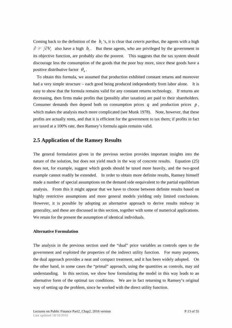
2.5 Application of the Ramsey Results The general formulation given in the previous section provides important insights into the nature of the solution, but does not yield much in the way of concrete results. Equation (25) does not, for example, suggest which goods should be taxed more heavily, and the two-good example cannot readily be extended. In order to obtain more definite results, Ramsey himself made a number of special assumptions on the demand side eequivalent to the partial equilibrium analysis. From this it might appear that we have to choose between definite results based on highly restrictive assumptions and more general models yielding only limited conclusions. However, it is possible by adopting an alternative approach to derive results midway in generality, and these are discussed in this section, together with some of numerical applications. We retain for the present the assumption of identical individuals. Alternative Formulation The analysis in the previous section used the “dual” price variables as controls open to the government and exploited the properties of the indirect utility function. For many purposes, the dual approach provides a neat and compact treatment, and it has been widely adopted. On the other hand, in some cases the “primal” approach, using the quantities as controls, may aid understanding. In this section, we show how formulating the model in this way leads to an alternative form of the optimal tax conditions. We are in fact returning to Ramsey’s original way of setting up the problem, since he worked with the direct utility function.


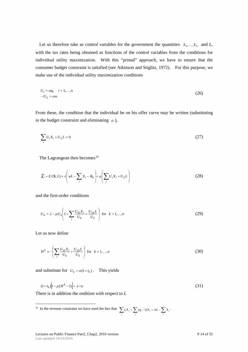
Let us therefore take as control variables for the government the quantities nXX ,,1 and L,

with the tax rates being obtained as functions of the control variables from the conditions for individual utility maximization. With this “primal” approach, we have to ensure that the consumer budget constraint is satisfied (see Atkinson and Stiglitz, 1972). For this purpose, we make use of the individual utility maximization conditions

wUniqU

L

iiα

α=−

== ,,1 (26)

From these, the condition that the individual be on his offer curve may be written (substituting in the budget constraint and eliminating α ),

∑ =+i

Lii LUXU 0 (27)

The Lagrangean then becomes10

++

−−+= ∑∑

iLii

ii LUXURXwLLU µλ 0),(XL (28)

and the first-order conditions

nkU

LUU

XUUUi k

Lk

k

iikkk ,,1for 1 =

++−= ∑µλ (29)

Let us now define

nkU

LUU

XUHi k

Lk

k

iikk ,,1for =

+−≡ ∑ (30)

and substitute for )1( kk tU += α . This yields

[ ] αλµ /)1(1)1( =−−+ k

k Ht (31)

There is in addition the ondition with respect to L

10 In the revenue constraint we have used the fact that ∑∑∑ −=−=

ii

iii

iii XwLXqXt )1( .


++−−= ∑

i L

LL

L

iiLLL U

LUU

XUUwU 1µλ (32)

If we define the corresponding expression

+−≡ ∑

i L

LL

L

iiLLU

LUU

XUH (33)

and substitute wUL α−= , we obtain

ααλµ −

=− )1( LH (34)

Eliminating µ between (31) and (33) gives11

−

−−=

+ L

Lk

k

k

HHH

tt

11 λαλ (35)

While this equation does not in general provide an explicit formula for the optimal tax rate

(since the terms kH depend on the tax rates), it does allow us to draw a number of conclusions about the optimal structure. (1) the partial equilibrium results can be seen as polar cases of this formula. Suppose on the

one hand that LH− tends to infinity, which corresponds to a completely inelastic supply of labour ∞→− LLU ; then the limit of (35) is a uniform tax on all goods at rate ααλ /)( −=tk .

Since we have seen that a uniform rate of tax on all goods is equivalent to a tax on labour alone, this corresponds to the conventional prescription that a factor in completely inelastic supply should bear all the tax.

(2) On the other hand, if LH tends to zero, we have the case of a completely elastic supply of labour (constant marginal utility of income). If in addition we assume that 0=ijU for

ji ≠ we have the conditions required for the validity of partial equilibrium analysis (no

income effects and independent demands). Since12

11 Equation (35) can also be obtained from the results of the previous section by inverting Eq. (25). For an

alternative approach using the Antonelli matrix, See Deaton (1979). 12 Differentiating kk qU α= where α is by assumption constant, and dividing by α .


−

−=

∂∂

L

Lk

k

kkk

HHH

qXU

1α implies d

k

kHε1

= (36)

The optimal tax

dk

k

k

k Ht

tελ

αλλαλ 1

1−

=−

=+

(37)

Solving for tk yields

αλλεαλ+−

−= d

kkt (38)

This shows that the formula (35) may be seen as a “weighted average” of two polar tax systems:

the uniform tax and taxes proportional to kH . Where between these two extremes the optimal tax system depends on LH . This tax is corresponding the Ramsey rule. (3) the formulation (35) suggests one case where the results may be particularly simple – that

where the utility function is directly additive. This implies that there exists some monotonic transformation of the utility function such that 0=ijU for ji ≠ . Since kH is

invariant with respect to such transformations13, this means that

k

kkkkU

XUH −= (39)

But by differentiating the first-order conditions for utility maximization, we can see that this is inversely proportional to the income elasticity of demand for k (defined M

kk MX ε=∂∂ ):

MU

Mq

MXU kk

kkk ∂

∂=

∂∂

=∂∂ α

αα 1 (40)

rearrange,

13 Suppose U is replaced by )(UG ; then jiijijii UUGUGGUGG ''',' +== . This means that

∑∑∑ −

−=

−=

iii

i k

iik

i k

iikk XUGG

UXU

GXG

H'''

But the second term disappears (using the budget constraint) establishing that kH is invariant.


Mk

kkM

XH

εα

α1

∂∂

− (41)

We have therefore the interesting result that when the utility function is directly additive, the optimal tax rate depends inversely on the income elasticity of demand. Necessities should be taxed more heavily than luxuries. This has important implications for the conflict between equity and efficiency, which are discussed further below. Direct additivity is a restrictive assumption; it is however considerably less restrictive than the assumptions required for partial

equilibrium analysis to be valid (for 0≠LH , direct additivity does not imply zero cross-price effects). Moreover, direct additivity is assumed in many demand studies, e.g., the linear expenditure system.

Finally, the primal approach adopted in this section has been used by Deaton (1979) to

discuss the conditions under which the optimal structure is uniform. He shows that the optimal tax conditions are identical for all goods if there is implicit separability between leisure and goods; i.e., where the expenditure function can be written ]),,(,[ UUfwe q . Combined with

weak separability between goods and leisure, this implies unitary expenditure elasticities (Sandmo, 1974a) 14 . In considering these results, the earlier qualification concerning non-uniqueness of the first-order conditions should be borne in mind: the fact that the right-hand sides of (35) may be equal for two goods does not necessarily imply uniformity.

2.6 Extension of the Ramsey Model to Many Households15 Once we start considering many persons/households in an economy, we need to define how to formulate social welfare as a representative of individual utilities, i.e. social welfare function. 1. The minimal state [Nozick (1974) Anarchy, State and Utopia], limited to the narrow

functions of protection against force, theft, fraud, enforcement of contract and so on is justified. Any more extensive state will violate person’s right not to be forced to do certain things is unjustified. The initial position taken by Nozick is a state of nature or anarchy. In this anarchy situation, there is a limited recognition of the rights of others, in sufficient to allow peaceful co-existence and Nozick argues that a dominant agency supplying protective services will emerge. This agency, because of free-rider problems has to adopt coercive taxation to

14 Sandmo shows that it implies equal compensated elasticities with respect to the wage. See also Sadka (1977).

The earlier statement in Atkinson and Stiglitz (1972, p.105) was unclear, although it was not intended to carry the interpretation placed on it by Sadka.

15 This part draws from Atkinson and Stiglitz (1980) pp.336-343.


finance the operation. Hence the minimal or ‘night watchman’ justification for the state. The minimal state offers only one public good – protection against violence, theft, and fraud – and the enforcement of contracts. Redistributive activity is limited to the financing of this minimal collective outlay.

2. Unanimity The minimal state is to allow the government to carry out unanimously approved activities. No violation of individual rights is involved.

3. Pareto efficiency The minimal state can approve Pareto improvements, i.e., to make at least one person better off and no one worse off. A Pareto efficient allocation is one where no Pareto improving move can be made.

4. Individualistic Social Welfare Functions The standard procedure for arriving at a complete ordering is to postulate a Paretian social welfare function. This function is Paretian in the sense of respecting individual valuations. W(U1,U2,U3, …UH) where Uh denotes the utility of individual/household h.

Two classes of social welfare functions are most well known.

1) The Benthamite objective of maximizing the sum of individual utilities, i.e. any positive linear transformation of

W = u1+ u2 + u3 + … + uH (42)

(Utilitarian social welfare functions) 2) The Rawlesian objective of maximizing the welfare of the worse-off individual

(maxi-min)

W Uh

h= min( ) (43)

These two are, in fact, special cases of the isoelastic formulation

( )[ ]∑ −−

=−

k

vhUv

W 11

1 1 (44)

Where the Benthamite case is v = 0 and the Rawlesian case is v → ∞. Note that Rawls [(1971) A theory of Justice ] considers the choices made in an initial position (original


position) which is defined such that people have no knowledge of their social position or preferences. This ‘veil of ignorance’ is assumed to ensure that the choice of moral principles is impartial or just; it is asserted that the decision made by people in that hypothetical position are an acceptable basis for a theory of justice. 5. Non-Individualistic Social Welfare Functions

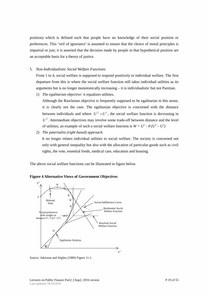
From 1 to 4, social welfare is supposed to respond positively to individual welfare. The first departure from this is where the social welfare function still takes individual utilities as its arguments but is no longer monotonically increasing – it is individualistic but not Paretian. 1) The egalitarian objective: it equalizes utilities.

Although the Rawlesian objective is frequently supposed to be egalitarian in this sense, it is clearly not the case. The egalitarian objective is concerned with the distance

between individuals and where 12 UU > , the social welfare function is decreasing in 2U . Intermediate objectives may involve some trade-off between distance and the level

of utilities, an example of such a social welfare function is W = U1 - θ (U2 – U1) 2) The paternalist (right based) approach.

It no longer relates individual utilities to social welfare. The society is concerned not only with general inequality but also with the allocation of particular goods such as civil rights, the vote, essential foods, medical care, education and housing.

The above social welfare functions can be illustrated in figure below. Figure 4 Alternative Views of Government Objectives

Source: Atkinson and Stiglitz (1980) Figure 11-1.

U2

U1

T

N’C

B

W

R

D

D

45º

•

•

•

• ••

•

•

•

Egalitarian Solution

Rawlsian SocialWelfare Function

Benthamite SocialWelfare Function

Social Indifference Curve

N

MinimalState

Social preferencewith weight on

distance U1-θ(U1- U2)


Which social welfare function you choose? Let’s extend the Ramsey model to many households case16. The economy is consist of H households. Each household h is described by an indirect utility function.

Uh = Uh (q1, …, qn, y) (45) These functions vary amongst the households.

Writing hn

hh xxx ,...,, 21 for the consumption demands from h, the government revenue constraint

is given by

∑∑= =

=n

i

H

h

hii xtR

1 1

(46)

Social welfare function is defined on the vector of indirect utilities

W = W (U1, U2, …, UH) (47) The government’s maximization problem is to maximize (47) subject to (46). It can be expressed in terms of the Lagrangean

−+= ∑∑

= =

n

i

H

h

hii

h RxtUWL1 1

)( λ (48)

The first-order conditions for the choice of the tax rate on good k, is

h

H

h

h

kkh

h

H

ih

H

i

nih

k

wu

uq

x t xq= = ==

+ +

=∑ ∑∑

1 1 11

0Σ∂∂

∂∂

λ∂∂

(49)

With Roy’s identity, the first term of (49) can be written

16 This part draws from Myles (1995, pp.108-111).


∂∂

∂∂

∂∂

αwu

uq

wu

xhh

H h

kh

h

Hh

kh

= =∑ ∑= −

1 1

(50)

and define

hh

h

uw αβ

∂∂

= (51)

where β h is the social marginal utility of income accruing to household h. αh is the marginal utility of income for h. Employing the definition of β h , (49) becomes,

β λ∂∂

h

h

H

kh

kh

iih

kh

H

i

n

h

H

x x t xq= ===

∑ ∑∑∑= +

1 111

(52)

Substituting from the Slutsky equation

∂∂

∂∂

xq

s x xy

ih

kikh

kh i

h

h

= − (53)

into (52) and rearranging gives the Ramsey rule for many households

t s

x

x

x

t xy

x

x

ih

H

kih

i

n

kh

h

H

hkh

h

H

kh

h

H

iih

hi

n

kh

h

H

kh

h

H==

=

=

=

==

=

∑∑

∑

∑

∑

∑∑

∑= − +

11

1

1

1

11

1

1 1λ

β∂∂

(54)

(54) can be expressed as

t s Hxx

t xy

xih

H

kih

i

n

k

hkh

h

H

ii

nih

hkh

h

H

==

=

= =∑∑

∑∑ ∑= − − −

11

1

1 1

β

λ∂∂

(55)


where xx

Hk

kh

h

H

= =∑

1 is the mean level of consumption of good k.

Define

b t xy

hh

ii

nih

h

= +=∑β

λ∂∂1

(56)

bh is Diamond’s net social marginal utility of income measured in terms of government revenue.

It is net in the sense that it measures both the gain in social welfare β h due to an increase in income to h and the increase in tax payments of h due to this increase in income. Thus bh involves both equity and efficiency effects. Using (56), (55) can be rearranged to give

t s

x

bH

xx

ih

H

kih

i

n

kh

h

H

hkh

kh

H==

=

=

∑∑

∑∑= − −

11

1

1

1 (57)

This is the alternative Ramsey rule for many households. The Ramsey rule (57) implies that the reduction in demand is smaller: (i) the more the good is consumed by individuals with a high bh (ii) the more the good is consumed by individuals with

a high marginal propensity to consume taxed goods ( )x xkh

k .

In other words, the optimal commodity tax rule for many households illustrates aspects of the efficiency/equity trade-off by the manner in which the reduction in demand for a good is related to the social importance of the major consumers of that good and their general contribution to the tax revenue. As is always the case with the Ramsey rule, it remains very general to obtain detailed results on the optimal tax structure, we need to make more specific assumptions about the nature of differences between individuals and the form of the utility function.

2.7 Empirical Studies of Optimal Consumption Taxation Empirical analysis of optimal tax rates is concerned with two issues: (1) The optimal tax rules derived theoretically suggest general observations about the structure of optimal taxes but they


do not have precise implications. Empirical analysis can be seen as providing a check on the interpretations and a means of investigating them further. (2) Empirical analysis can provide practical policy recommendations. To do this, the tax rules must be capable of being applied to data and the values of the resulting optimal taxes calculated. As Deaton (1981) notes, “present theoretical formulae do not yield clear-cut results except in special cases and it has recently become clear that optimal rates depend crucially on the detailed structure of consumer preferences” (p.1245). For example, Atkinson and Stiglitz (1976) show that with an optimal nonlinear income tax, discriminatory commodity taxes are only necessary to the extent that individual commodities are not weakly separable from leisure. “Econometricians estimating commodity demand and labor supply equations make generous use of separability assumptions to enable estimation at all. In consequence, it is likely that empirically calculated tax rates, based on econometric estimates of parameters, will be determined in structure, not by the measurements actually made, but by arbitrary, untested (and even unconscious) hypotheses chosen by the econometrician for practical convenience” (Deaton, ibid.)17. To remedy this situation, and as a prelude to fruitful empirical work, it is necessary to have more explicit understanding of how preference structure affects optimal tax rates. The major empirical modifications are as follows.

(1) The many consumers economy. (2) Consumption demand and labor supply are not separable. If they are, income tax and

commodity tax can be treated separately. If they are not, both taxes must be determined jointly.

(3) The relationship between consumption demand and income (known as the Engel Curve) can be non-linear.

Indeed, the importance of assumptions about consumer preferences for the ‘optimal’ commodity tax rates is now widely accepted in the literature [see, Deaton (1981)]. For example, it is well known that commodity taxes will be uniform if (i) labor supply is completely inelastic, or (ii) consumption is weakly separable from leisure, and the consumption indifference map is homothetic or Engel curves are linear or an optimal non-linear income tax is allowed for. One ought to emphasize here that the uniformity result is only valid within a framework where people have identical preferences and differ only in their earning power which consists of one factor. None of the above requirements for uniform commodity taxes is likely to be met in practice. 17 Many econometric works on consumer demand is based on the Linear Expenditure System (LES) in which

demands are additively separable and the linear Engel curve or linear (quasi-homothetic) preferences the theoretical attraction of linear preferences lies in the aggregation theorems of Gorman, while the empirical attraction is ease of interpretation and estimation of the underlying parameters.


There exists a large body of empirical evidence which suggests that leisure is not weakly separable from goods, the Engel curves are not linear [Blundell and Ray (1984)], and the goods utility function is not additively separable, for less homothetically so. In the Indian context, Ray (1986 a,b) provides evidence of non-homothetic and non-separable commodity demand functions with non-linear Engel curves. Further evidence of non-linear Engel curves on time series of national accounts data of some developing countries is also available.

Demand models play an important role in the evaluation of indirect tax policy reform. We argue that for many commodities, standard empirical demand models do not provide an accurate picture of observed behavior across income groups. Our aim is to develop a demand model that can match patterns of observed consumer behavior while being consistent with consumer theory and thereby allowing welfare analysis.

The distributional analysis of commodity tax policy requires the accurate specification of both price and income effects. Crude utility-based demand models such as the linear expenditure system, however, impose strong and unwarranted restrictions on price elasticities (Deaton (1974)). Recognition of this spawned a large literature, first on flexible demand systems and later on semiparametric and nonparametric specifications of demands. Except for the estimation of Engel curve, these nonparametric methods are generally series rather than kernel based (see Barnett and Jonas (1983) or Gallant and Souza (1991) because of the difficulty of imposing utility-derived structure (such as Slutsky symmetry) on kernel estimators.

Since incomes vary considerably across individuals and income elasticities vary across goods, the income effect for individuals at different points in the income distribution must be fully captured in order for a demand model to predict responses to tax reform usefully. Indeed, the study of the relationship between commodity expenditure and income (the Engel curve) has been at the center of applied microeconomic welfare analysis since the early studies of Engel (1895), Working (1943), and Leser (1963). But a complete description of consumer behavior sufficient for welfare analysis requires a specification of both Engel curve and relative price effects consistent with utility maximization. An important contribution of the Muellbauer (1976), Deaton and Muellbauer (1980), and Jorgenson et al. (1982) studies was to place the Working – Leser Engel curve specification within integrable consumer theory.

We derive a new class of demand systems that have log income as the leading term in an expenditure share model and additional higher order income terms. This preserves the flexibility of the empirical Engel curve findings while permitting consistency with utility theory and is shown to provide a practical specification for demands across many commodities, allowing flexible relative price effects. We show that the coefficients of the higher order income terms in these models must be price dependent and that these higher order terms have to include a quadratic logarithmic term. The demands generated by this class are shown to be


rank 3 which, as proved in Gorman (1981), is the maximum possible rank for any demand system that is linear in functions of income. The quadratic logarithmic class nests both the Almost Ideal (AI) model of Deaton and Muellbauer and the exactly aggregable Translog model of Jorgenson et al. (1982). Unlike these demand models, however, the quadratic logarithmic model permits goods to be luxuries at some income levels and necessities at others. The empirical analysis we report suggests that this is an important feature.

Having established the Engel curve behavior, a complete demand model is estimated on a pooled FES data set using data from 1970 to 1986. This model produces a data-coherent and plausible description of consumer behavior. The specific form we propose – the Quadratic Almost Ideal Demand System (QUAIDS) – is constructed so as to nest the AI model and have leading terms that are linear in log income while including the empirically necessary rank 3 quadratic term. Regularity conditions for utility maximization, such as Slutsky symmetry, can be imposed on our model and are not statistically rejected. Regularity constraints involving inequalities cannot hold globally for any demand system such as ours, which allows some Engel curves to be Working – Leser, because at sufficiently high expenditure levels a budget share that is linear must go outside the permitted zero-to-one range 18 . Despite this, negative semidefiniteness of the Slutsky matrix is found to hold empirically in the majority of the sample, with the exceptions being the very high income households.

More specifically, let x equal deflated income, that is, income divided by a price index. One convenient feature of the AI model is that the coefficients of ln x in the budget share equations are constants. Our theorem 1 shows that any parsimonious rank 3 extension must be quadratic in ln x . Given this it would be convenient19 if a rank 3 specification could be

constructed in which the coefficients of both ln x and 2)(ln x were constants. We find that a surprising implication of utility maximization is that constant coefficients are not possible in such models – the coefficients of 2)(ln x must vary with prices. The QUAIDS model we propose makes this required price dependence as simple as possible.

We will estimate the QUAIDS Demand Function. Let us first define notations. Demand share is given

i

iii y

qPw = , ∑=

=n

iii qPy

1

(58)

Following Banks et al. (1997), to derive the QUAIDS Demand Function from Indirect Utility

18 Some globally regular demand systems do exist (Barnett and Jonas (1983) and Cooper and McLaren (1996), for

example), but these are all examples of fractional demand systems, and none with rank higher than 2 have been implemented empirically.

19 It was shown by Blundell et al (1993) to empirically plausible.


Function

∑ ∑

∑ ∑+−+

−+−++=≠

iililiiii

n

jiiiijiijii

xpwy

pwyPPPw

εφβ

βγαα

22

110

)ln(ln

)ln(ln)ln(lnln (59)

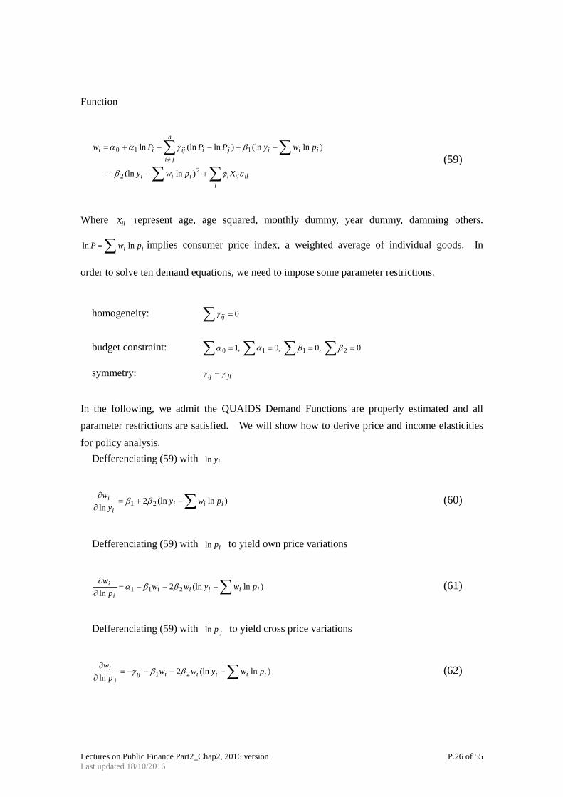
Where ilx represent age, age squared, monthly dummy, year dummy, damming others.

∑= ii pwP lnln implies consumer price index, a weighted average of individual goods. In

order to solve ten demand equations, we need to impose some parameter restrictions.

homogeneity: ∑ = 0ijγ

budget constraint: ∑∑∑∑ ==== 0 ,0 ,0 ,1 2110 ββαα

symmetry: jiij γγ =

In the following, we admit the QUAIDS Demand Functions are properly estimated and all parameter restrictions are satisfied. We will show how to derive price and income elasticities for policy analysis.

Defferenciating (59) with iyln

∑−+=∂∂

)ln(ln2ln 21 iii

i

i pwyy

wββ (60)

Defferenciating (59) with ipln to yield own price variations

∑−−−=∂∂

)ln(ln2ln 211 iiiii

i

i pwywwp

wββα (61)

Defferenciating (59) with jpln to yield cross price variations

∑−−−−=∂∂

)ln(ln2ln 21 iiiiiij

j

i pwywwp

wββγ (62)


A) Derivation of Income Elasticity

Income elasticity ie using i

iii y

qpw = , is obtained as follows

1−=∂

∂

i

i

i

i

i

e

yy

ww

Rearranging this equations,

11ln

−=•∂∂

iij

i ewy

w (63)

with equation (60), we can rewrite

∑ +−+= 1))ln(ln2(121 iii

ii pwy

we ββ (64)

This is the income elasticity. B) Derivation of Price Elasticity Price elasticity can be devided into own price elasticity iiε and cross price elasticity ijε .

Own Price Elasticity

∑−−−=

•∂∂

=∂

∂

=

)ln(ln2

1ln

21 iiii

i

ii

i

i

i

i

i

ii

pwyw

wpw

pp

ww

ββα

ε (65)

Cross Price Elasticity It is defined as follows


1+=∂

∂

ij

i

i

i

i

pp

ww

ε (66)

That is,

11ln

+=•∂∂

ijij

iwp

wε (67)

Using by (62), we can rewrite

1)ln(ln2 21 −−−−−= ∑ iiii

j

i

j

i

ijij pwy

ww

ww

wββ

γε (68)

C) Derivation of Price Elasticity with Income Compensation

)( 1 jiww

we ii

iiiicii =+=+=

αεε (69)

)( 1 jiww

we ii

ijjiij

cij ≠−+−=+=

γεε (70)

This ends all preparations.

Empirical Results and Interpretation Empirical research is conducted by using Family Income and Expenditure Survey, conducted by Ministry of Internal Affairs and Communications, Statistics Bureau from January 1985 to April 2012, 328 monthly data for the two or more member households. Price data are taken from Consumer Price Indexes (2010 base year) by different consumption categories20.

After scrutiny on ten consumption categories, housing related expenditure turns out to be heterogeneous to the other categories. We estimate nine consumer demand equations by 3SLS, omitting housing related expenditure21. Parameter restrictions we impose are 48 all-together. 20 These data are downloadable from the homepage of National Statistics Center. 21 Due to the budget constraint for the simultaneous equations, 9 demand equations out of ten determine the rest, it

is desirable to estimate 9 simultaneous equations.


50 parameters are to be estimated for each equation. Figure 4 shows the Engel curves by categories. Figure 4: Engel Curve by Categories

.18

.2.2

2.2

4.2

6.2

8

7.8 8 8.2 8.4 8.6realincome

foodshare Fitted values

.04

.05

.06

.07

.08

7.8 8 8.2 8.4 8.6realincome

housingshare Fitted values

.04

.06

.08

.1

7.8 8 8.2 8.4 8.6realincome

fuelshare Fitted values

.02

.03

.04

.05

.06

7.8 8 8.2 8.4 8.6realincome

furnitureshare Fitted values

.02

.04

.06

.08

.1

7.8 8 8.2 8.4 8.6realincome

clothingshare Fitted values

.02

.025

.03

.035

.04

.045

7.8 8 8.2 8.4 8.6realincome

medicalshare Fitted values

.08

.1.1

2.1

4.1

6.1

8

7.8 8 8.2 8.4 8.6realincome

transshare Fitted values

.02

.04

.06

.08

.1.1

2

7.8 8 8.2 8.4 8.6realincome

educshare Fitted values

.08

.09

.1.1

1.1

2.1

3

7.8 8 8.2 8.4 8.6realincome

recreationshare Fitted values

.2.2

5.3

.35

7.8 8 8.2 8.4 8.6realincome

othershare Fitted values

A standard Engel curve would be upward sloping. Engel curves of furniture, clothing and footwear and other expenditure are indeed upward sloping. All demand shares seem to illustrate quadratic relationship with real income. This fact may justify to use the Quadratic Almost Ideal Demand System (QUAIDS). Figure 5 illustrates the relationship between the price (vertical axis) and the demand share (horizontal axis). It can be interpreted as a kind of consumer demand function. A normal consumer demand function must be downward sloping. Those of housing, fuel and electricity, medical expenditure, education and recreation look like upward sloping. It can be said that the relationships between the price and demand share are not so clear overall.


Figure 5: Consumer Demand Curve by Categories .1

8.2

.22

.24

.26

.28

4.45 4.5 4.55 4.6 4.65foodp

foodshare Fitted values

.04

.05

.06

.07

.08

4.3 4.4 4.5 4.6housp

housingshare Fitted values

.04

.06

.08

.1

4.45 4.5 4.55 4.6 4.65 4.7fuelp

fuelshare Fitted values

.02

.03

.04

.05

.06

4.5 4.6 4.7 4.8 4.9 5furnip

furnitureshare Fitted values

.02

.04

.06

.08

.1

4.4 4.5 4.6 4.7clothp

clothingshare Fitted values

.02

.025

.03

.035

.04

.045

4.3 4.4 4.5 4.6 4.7medicalp

medicalshare Fitted values

.08

.1.1

2.1

4.1

6.1

84.58 4.6 4.62 4.64 4.66 4.68

transp

transshare Fitted values

.02

.04

.06

.08

.1.1

2

4 4.2 4.4 4.6 4.8educp

educshare Fitted values

.08

.09

.1.1

1.1

2.1

3

4.5 4.6 4.7 4.8recreationp

recreationshare Fitted values

.2.2

5.3

.35

4 4.2 4.4 4.6 4.8otherp

othershare Fitted values

Table 1 shows that, observing z-values in each equation, own price elasticities of food and medicine are significantly negative while those of other seven equations are insignificant, thus interpreted as zero coefficients. We could interpret that negative coefficient restriction is satisfied, given no significantly positive coefficient exists. Table 1 also indicates that the model specification is appropriate as the overall model fits very well and the parameter values are reasonable22. Cross price elasticity may take any values (either positive or negative), it is limited to find statistically significant coefficients and it is also difficult to interpret substitution effects between different consumption categories. Table 2, Panel A reports the price elasticities for compensated (taking into account of income elasticity) demand. Panel B reports those for uncompensated (not taking into account of income elasticity) demand. Table 2 confirms that the own price elasticities for food and medical expenditures are significantly negative while all other own price elasticities are insignificant, regardless of positive and negative coefficient values. Let us consider why most own price elasticities are not significant. It is conventional to assume that insignificant parameter values of interests imply misspecifications of functional

22 We must admit that the parameter values and sign conditions are not stable over different estimation periods and

estimation methods. In other words, the results reported here are not necessarily robust.


forms, omitted variables, strong parameter restrictions, among others. Our purpose is to identify consumption items that can be applied reduced tax rate by estimating the own price elasticities. It is not our objective to implement the Ramsey rule for all consumption items23. In fact, the price levels do not fluctuate significantly over time after 2000 because of zero inflation or subtle deflation rates, it would be very difficult to identify the statistical relationship between the price and consumer demand. In other words, it is not strange to find that many consumption items have zero coefficients on the own price elasticities. In addition, administratively it is a very simple result that a single tax rate should be applied except for two items.

23 If all own price elasticities are significantly negative, following the Ramsey rule, the multiple tax rates on

different consumption items are to be introduced. Given the tax revenue, it would be quite complex to determine the multiple rates in practice.

Lectures on Public Finance Part2_Chap2, 2016 version P.32 of 55

Table 1: Estimation of Consumers Demand Equation by 3SLS

Food Fuel Furniture Clothing Medical Transport Education Recreation Others Coef Z Coef Z Coef Z Coef Z Coef Z Coef Z Coef Z Coef Z Coef Z

foodp -0.058 -2.16 -0.003 -0.24 0.012 0.79 0.065 4.33 -0.005 -0.51 0.011 0.56 -0.025 -1.68 0.004 0.21 -0.002 -0.09 fuelp -0.003 -0.24 0.022 1.20 0.018 1.77 -0.022 -2.24 -0.005 -0.80 0.020 1.54 -0.027 -2.63 -0.008 -0.66 -0.021 -1.22 furnip 0.012 0.79 0.018 1.77 0.019 0.66 0.020 1.27 0.002 0.21 -0.048 -2.61 0.002 0.20 -0.005 -0.26 0.004 0.31 clop 0.065 4.33 -0.022 -2.24 0.020 1.27 0.002 0.10 0.005 0.55 -0.044 -2.42 -0.006 -0.47 -0.029 -1.65 0.010 0.54 medip -0.005 -0.51 -0.005 -0.80 0.002 0.21 0.005 0.55 -0.024 -1.41 0.014 1.25 0.000 -0.03 0.023 2.11 -0.011 -1.01 transp 0.011 0.56 0.020 1.54 -0.048 -2.61 -0.044 -2.42 0.014 1.25 0.024 0.71 -0.052 -2.14 0.067 3.11 0.008 0.24 educp -0.025 -1.68 -0.027 -2.63 0.002 0.20 -0.006 -0.47 0.000 -0.03 -0.052 -2.14 0.002 0.10 0.013 0.83 0.093 3.96 recrep 0.004 0.21 -0.008 -0.66 -0.005 -0.26 -0.029 -1.65 0.023 2.11 0.067 3.11 0.013 0.83 0.015 0.47 -0.080 -3.74 otherp -0.002 -0.09 0.004 0.31 -0.021 -1.22 0.010 0.54 -0.011 -1.01 0.008 0.24 0.093 3.96 -0.080 -3.74 -0.001 -0.03 realincome -0.489 -2.16 -0.380 -2.48 -0.315 -1.79 -0.487 -2.54 -0.081 -0.73 1.292 2.91 1.317 3.83 -0.103 -0.45 -0.754 -1.69 realincomesq 0.021 1.55 0.021 2.24 0.020 1.93 0.032 2.81 0.004 0.66 -0.075 -2.83 -0.077 -3.76 0.006 0.43 0.048 1.81 age 0.139 3.90 0.008 0.34 0.079 2.82 0.058 1.88 -0.024 -1.38 0.067 0.94 -0.009 -0.16 0.002 0.06 -0.324 -4.57 agesq -0.001 -3.78 0.000 -0.20 -0.001 -2.83 -0.001 -1.92 0.000 1.38 -0.001 -1.02 0.000 0.10 0.000 -0.08 0.004 4.62 _cons -0.140 -0.11 1.475 1.74 -0.610 -0.63 0.587 0.56 1.064 1.74 -6.951 -2.83 -5.329 -2.81 0.462 0.37 10.443 4.24 monthlydummy Yes Yes Yes Yes Yes Yes Yes Yes Yes yeardummy Yes Yes Yes Yes Yes Yes Yes Yes Yes R-squared 0.969 0.968 0.865 0.960 0.915 0.912 0.917 0.881 0.923 Chi-squared 10028.17 9862.06 2007.42 7666.18 3438.11 3477.80 3790.53 2442.61 4037.21 Observation 328 Parameters 50

Estimation of Simultaneous equations is conducted on 9 items (excluding housing) by 3SLS.

Own price is logarithm of own price, other price is a difference of log of other price minus log of own price. For example, fuel price (fuelp) in Food demand equation is defined as

( )fuelpfoodpInInfuelpInfoodpfuelp =−=


Table 2: Price Elasticity of Consumer Demand Panel A Compensated Case

Food Fuel Furniture Clothing Medical Transport Education Recreation Others Food -0.325 -1.886 -3.037 -3.973 -1.097 1.227 4.986 -1.008 -1.385 Fuel -1.008 0.141 -1.981 -1.066 -0.901 -0.569 0.949 -0.910 -1.121 Furniture -1.063 -1.454 0.303 -1.635 -1.111 -0.237 -0.180 -0.946 -0.978 Clothing -1.301 -0.862 -1.975 -0.358 -1.229 -0.044 -0.662 -0.695 -1.131 Medical -0.989 -1.037 -1.290 -1.333 -0.840 -0.821 -0.280 -1.234 -1.011 Transport -1.089 -1.827 -0.535 -1.131 -1.611 1.393 2.928 -1.679 -1.242 Education -0.909 -0.745 -1.481 -1.299 -1.049 -0.029 1.206 -1.124 -1.460 Recreation -1.047 -1.257 -1.583 -1.212 -1.883 -0.595 1.079 0.729 -0.850 Other -1.073 -2.113 -2.283 -3.113 -0.933 1.540 3.019 -0.136 -0.436 Budget Elasticity -0.960 -4.812 -6.992 -6.998 -1.434 10.649 24.880 0.054 -1.598

Panel B Uncompensated Case Food Fuel Furniture Clothing Medical Transport Education Recreation Others

Food -0.108 -0.777 -1.447 -2.382 -0.766 -1.229 -0.761 -1.020 -1.019 Fuel -0.949 0.420 -1.549 -0.633 -0.817 -1.205 -0.511 -0.913 -1.023 Furniture -1.030 -1.279 0.542 -1.394 -1.059 -0.619 -1.089 -0.948 -0.922 Clothing -1.249 -0.585 -1.594 0.009 -1.146 -0.657 -2.070 -0.697 -1.044 Medical -0.959 -0.893 -1.074 -1.113 -0.798 -1.139 -1.030 -1.236 -0.962 Transport -0.970 -1.249 0.332 -0.245 -1.444 0.129 -0.075 -1.687 -1.043 Education -0.857 -0.495 -1.012 -0.919 -0.973 -0.592 -0.009 -1.126 -1.373 Recreation -0.953 -0.787 -0.903 -0.522 -1.745 -1.623 -1.373 0.167 -0.694 Others -0.828 -0.872 -0.509 -1.356 -0.561 -1.211 -3.203 -0.149 -0.034 Budget Elasticity -0.960 -4.812 -6.992 -6.998 -1.434 10.649 24.880 0.054 -1.598


Table 3 shows that effective tax rates on medical and educational expenditures are very low. The own price elasticity of medical expenditure is sensitive to the price change and it is necessary item to pursue the healthy life. It is reasonable to admit the reduced tax rate for medical expenditure. On the other hand, the own price elasticity of education is statistically zero and thus the price change does not affect the education demand. At the same time, educational expenditure has a very strong income effect, i.e. the income elasticity of education is as high as 24.88. What does it mean? Table 3 Effective Tax Rates

Items Oshio（2010） Murakami（2006） Murasawa, Yuda

and Iwamoto（2005）

Food 5.86 7.10 7.23 Residence 2.12 1.66 1.68 Fuel 5.49 5.36 5.33 Furniture 4.76 4.76 4.76 Clothing 4.76 4.76 4.76 Medical 1.91 2.09 2.17 Transport 9.59 10.70 11.25 Education 1.04 1.09 1.20 Recreation 4.76 5.07 4.83 Others 7.36 8.65 7.09 Total 5.61 6.50 NA Research Year 2008 2003 2000

Source: Oshio (2010) Table 4-2, p.99.

It is well known that educational expenditures such as tuition, entrance examination fees, and textbooks are tax exempt, but other educational expenditures are taxed. Nevertheless, given tuition occupies a high proportion of educational expenditure, it is understandable to have the effective tax rate of education is approximately 1.0%. Under the regime of Democratic party (September 2009 – December 2012), they tried to introduce the free public high school education, to begin with, and to implement the education system from the primary to high schools that guarantees every student, regardless of their parent’s income, to be able to receive their education . However, the high income elasticity of education implies that the higher income households spend more on education. That is, considering the quality difference between the public and the private schools with heavy subsidies to the public schools, the parents have a strong incentive to give their children high quality private education. To do so, it is essential for children to participate the preparatory schools after the formal education. This fact may explain at least, to some extent, the high elasticity of education. In any case, it is required to study further the


taxation on education. The income elasticity is also high for transportation and communication expenditure. It is obvious that demand for automobile related expenditure is highly correlated with income level. Also zero price elasticity implies that such expenditure is highly habitual so that a high tax rate may not reduce its demand. As we saw in Table A, the effective tax rate for transportation and communication is above 10%. This expenditure also serves as the base of environmental tax. The consumption tax rate reduction may apply to the items with negative but significant price elasticities. A very high portion of medical expenditure has been exposed to the zero rate or has exempted from the taxation. Only item that tax rate reduction can apply is food expenditure. As to food expenditure, alcohol tax has been imposed on liqueur and alcohol beverages so that the effective tax rate for food expenditure under the 5% VAT time has been 6-7%. The tax rate reduction for food expenditure would be justifiable24. Because of the Engel’s law, the share of food expenditure has been declining. Nevertheless, the share is still about 18%. It is not easy to allow for substantial revenue loss25. It will be politically complex issue as to which tax items should be raised to compensate the revenue losses from food expenditure. To be fair with the consumption tax system, it would be desirable not to apply the reduced rate for food expenditure.

Conclusions We have shown how to determine the practical consumption tax rates using the average statistics from Family Income and Expenditure Survey. The government is to apply the reduced rate for some items to accommodate/weaken the regressivity of consumption tax. We insist that the government should determine whether the reduced rate should be applied for which items according to the empirical evidences of own price elasticities derived from the appropriate consumer demand functions. The reduced rate should not be determined by the lobbying activities of some industries regardless of empirical evidences. As is clear from our investigation, the empirical evidences would turn out to be persuasive if an appropriate

24 It is a relatively straightforward to determine a single reduced rate (i.e. it is not multiple rates for multiple

expenditure items). We need to consider to what extent we could bear the revenue loss and to what level we could set a reduced rate.

25 Let us conduct a simple calculation for revenue losses. The total household consumption of food and non-alcohol beverages was 38.4 trillion yen in 2011 and the effective VAT rate was 0.0456. When consumption tax rate is raised from 5% to 10%, if we keep 5% for consumption of food and non-alcohol beverages and the tax efficiency remains the same, the tax revenue would be 1.75 trillion yen. If 10% is applied, the revenue would be double, 3.5 trillion yen. That is to say, the revenue losses are 1.75 trillion yen per annum. We consider the case in which all consumption of food and non-alcohol beverages were taxed at 5%, the revenue losses would be substantial even if we reduce number of food consumption items at the 5% rate. Alternatively, when it is raised from 5% to 8%, the consumption tax rate is kept fixed at the single rate of 8% for all items as it is now. When it is raised from 8% to 10%, if consumption of food and non-alcohol beverages remain at 8% while all other items are taxed at 10%, the revenue losses would be 0.7 trillion yen.


estimation of demand function is conducted. Our empirical methods are not free from criticisms. The data we use are the national average

of employee’s households with two or more members. The elasticity of labor supply is essentially low. As the optimal consumption tax literature shows, it is desirable to impose a single rate on these households. Our empirical results also support more or less a single rate. Alternatively we could argue that we shall design a tax policy under a specific social welfare function and individual preference parameters. In this case, we shall specify the empirical model by means of microdata. Some economists argue that we shall increase in progressivity of income tax schedule before increasing a consumption tax rate by pointing out some administrative problems of consumption tax. However, what public finance experts have observed and what many European countries have experienced with the income tax are the difficulty of capturing consolidated income due to plurality of employment styles and income sources. As is well known, the tax authority can relatively easily capture the income source of regular workers while it is very difficult to capture the income of self-employed workers such as farmers and irregular workers. Furthermore, it is also difficult to capture economic activities of moonlighting by the regular workers after their regular works. In order to overcome these difficulties, consumption tax or the general value added tax has been introduced. The tax authority is required to improve constantly the administrative obstacles of consumption tax. Compared with those with income tax as discussed above, these obstacles with consumption tax can be overcome. That is the main reason why we consider the consumption tax in this chapter. Many public finance experts argue that income tax revenue can be raised by recovering the progressivity of income tax schedule and by reducing the exemptions and deductions from the income tax base. We agree with this view and have shown elsewhere that it is empirically desirable to reduce income tax exemptions and deduction from the income tax base and to raise the top income tax rate a bit higher. The golden rule of taxation is to impose taxes on whichever the tax bases the taxpayers can afford to pay. Income tax as a direct tax is effective for the regular workers as it can be withheld at source. But this tax is not so effective for the unemployed, the elderly and the self-employed. The tax basis of income tax was narrowed by introducing various exemptions and deductions and by raising the threshold, in exchange of introduction of consumption tax. The co-existence of income and consumption taxes can be justified by the evidences we raise above.


Appendix 1 Introduction to Value Added Tax26 In this appendix, an attempt has been made to explain the meaning and characteristics of value added tax (VAT) and to indicate why it is to be preferred to the sales taxes levied on the gross sale value of commodities. Prior to embarking on this explanation, it will be useful to define value added and show how it can be measured. The gross output of goods and services produced in a country is measured in terms of the total value of all the commodities and services when they reach the hands of the final users, namely, consumers and investors (buyers of capital goods), after going through various stages of production, plus the value of exports. This measure of total output for a year is termed gross domestic product for the year and represents the sum of all values of goods and services produced in the country during the year. Now typically, each commodity passes through several stages of production and at each stage some value is created or added. The total value of a commodity as it reaches the hands of the final user is the sum of values created at the successive stages of production. The value added at each stage of production can be worked out (quantitatively) from the production account of the enterprise or producing unit concerned. That account for a year can be presented in the following way (in summary terms):

Receipts Rs Expenditure Rs Income from sale of output 10,000 Cost of bought out inputs 4,000 (=gross value of output) Wages and salaries 2,000 Rent 1,500 Interest 500 Depreciation 1,000 Surplus (Profits) 1,000 10,000 10,000 Gross value of output = Rs 10,000 Gross value added = gross value of output － cost of bought out inputs

= Rs 10,000 － Rs 4,000 = Rs 6,000 (It is assumed that there is no change in inventories.)

It may be noted that gross value added is equal to the sum of wages and salaries, rent, interest,

depreciation, and profits (net value added will exclude depreciation). Under VAT, the value added at each stage of production and distribution is equal to the total value embodied in a commodity, the VAT on a commodity amounts to a tax on just the total value of that commodity. By contrast, a sales tax on the total value of output or turnover falls on the value of inputs at successive stages unless the tax is confined to retail sales. Even the first point sales tax levied by most state governments has a base that includes the cost of current and capital inputs at successive stages of manufacturing. As has already been indicated, this

26 This appendix draws from Chelliah, Aggarwal, Purohit and Rao (2005).


results in cascading of tax burden and escalation of costs. Hence the need to adopt VAT, though it is necessarily a multi-point tax. Computation of VAT VAT can be computed in one of two ways: the subtraction method and the addition method. In the former the tax rate is applied to the difference between the value of output and the cost of inputs. In the addition method the value added is computed by adding all the payments to eh factors of production, viz., wages, rent, interest, and profits (as will be shown later, this method can be used only with the ‘income variant’ of VAT). In implementing VAT, most countries use an amended form of the subtraction method. The subtraction method of applying VAT may he described as I)t(OVAT −=

where t is the tax rate, O is the value of output, and I is the value of inputs. Now I)t(O − can be rewritten as I)(tO t− . That is, VAT can be collected as the difference between the tax

payable on output and the tax paid on inputs. This method of computing and collecting VAT is called the input tax credit method. Here, we shall discuss only the subtraction method and the input tax credit method. In a VAT, while the tax is levied and collected at every stage of production and distribution, it si to be ultimately borne by the final user of the good. This implies that tax inclusive price at any stage has to include taxes collected at all earlier stages. The input tax credit method achieves this by requiring the seller to collect tax on the entire value of output and retain the amount equivalent to the tax paid on purchases. However, in the subtraction method, at any stage, the tax is to be collected only on the value added at that stage. The taxes paid at the earlier stages would have to be a part of the cost of inputs, and the final price quoted by the seller would be a tax-inclusive price. The tax due at any stage is computed by using a formula as shown in Table A1.


Table A1 Computing VAT by Two Methods with a Uniform Tax Rate of 10 percent

Raw Materials Supplier Manufacturer Wholesaler Retailer Total

Economy The Economy Purchases --- 100 350 850 ---

Value Added 100 250 500 250 1100 Sales 100 350 850 1100 --- Input tax credit method

i. Sales 100 350 850 1100 2400 ii. Taxes collected 10 35 85 110 240 iii. Purchases 0 100 350 850 1100 iv. Taxes paid 0 10 35 85 130

VAT (ii - iv) 10 25 50 25 110 Price of the good = 100 + 10 = 350 + 35 = 850 + 85 = 1100 + 110

(i + ii) = 110 = 385 = 935 = 1210 Subtraction method

i. Sales 110 385 935 1210 ii. Purchases --- 110 385 935

Calculation of tax due )1.1(

1.)0110( ×−=

)1.1(1.)110385( ×−

= )1.1(

1.)385935( ×−=

)1.1(1.)9351210( ×−

=

Tax Due 10 25 50 25 110

Table A2 Wholesaling Stage is Subject to a 15 percent tax, and Rest to a 10 percent Tax

Raw Materials Supplier Manufacturer Wholesaler Retailer Total

Economy Effective

Rate of Tax The Economy Purchases --- 100 350 850 ---

Value Added 100 250 500 250 1100 Sales 100 350 850 1100 --- Input tax credit method

i. Sales 100 350 850 1100 2400 ii. Taxes collected 10 35 127.5 110 240 iii. Purchases 0 100 350 850 1100 iv. Taxes paid 0 10 35 127.5 130

VAT (ii - iv) 10 25 92.5 -17.5 110 10% Subtraction method

i. Sales 110 385 960 1235 ii. Purchases --- 110 385 960

Calculation of tax due )1.1(

1.)0110( ×−=

)1.1(1.)110385( ×−

= )1.1(

1.)385960( ×−=

)1.1(1.)9351235( ×−

=

Tax Due 10 25 75 25 135 12.3%

Exemptions and Zero Rating Under VAT, a distinction is made between exemption and zero rating. Exemption usually means exemption from tax on the value added of a commodity at a particular stage of production or distribution. If full exemption is desired, there should be zero rating of the commodity concerned. That is, a rate of zero should be imposed on the commodity against which rebate should be given for input taxes. This is a particularly useful tool for exports. In order to maintain the international competitiveness of a commodity, exports out of a tax jurisdiction can be relieved of all domestic taxes through zero rating. Exemptions are not desirable under VAT as they break the input tax credit chain. If this commodity re-enters the production process as an input for a taxable commodity, the problem of cascading reappears.


Also exemption from tax at one point does not mean total exemption because taxes on inputs at the earlier stages will remain embedded, leading to loss of transparency. Thus, an exemption does not imply a zero effective tax rate on the commodity. Exemptions should be kept to the minimum. Choosing a Base for VAT There are three possible variants of VAT, depending upon what macroaggregate the government wants to tax: gross income, net income- or consumption. In terms of the macro-aggregates, Gross Product = consumption + gross capital formation = gross value of output – all current inputs. A VAT on gross income would therefore treat both consumption and capital formation as final uses of the good; hence capital goods purchased by the dealer would not be treated as inputs. Input tax credit will not be available on taxes paid on capital goods. Net Income = consumption + gross capital formation － depreciation = gross income – depreciation = gross value of output – all current inputs － depreciation. A VAT on net income would therefore give credit for tax paid on current inputs and tax paid on capital goods to the extent attributable to depreciation of capital goods, in any given year. Under the ITC method, this implies that the credit for tax on capital goods will be spread over the life of the capital good. The consumption type VAT goes a step further in that only final consumption is treated as the final use of a good; full credit, therefore, is given for taxes paid on capital goods as well, in the year of purchase. Consumption = gross value of output – current inputs － gross capital formation Table A3 illustrates the calculation of VAT with three alternative bases. A tax on production or on income potentially distorts and discourages investment decisions, affecting the growth of the economy. A tax on income for instance, could alter consumer decisions in favour of present consumption, because it implies double taxation of savings27.

27 Savings are taxed at the time of saving and again the income from savings is taxed.


Table A3 Comparison of VAT on Alternative Bases Consumption of VAT at 10% Value of Output

(Rs) Consumption Type

(Rs) Income Type (Rs) Gross Product Type (Rs)

Intermediate inputs Output 200 20 20 20 Capital goods Output 150 15 15 15 Input 100 -10 -10 -10 Tax Paid 5 5 5 Consumption goods Output 300 30 30 30 Input 100 -10 -10 -10 Capital 150 -15 -1.5 Tax paid 5 18.5 20 Tax collection 30 43.5 45 Total consumption 300 Total income 435 Total production 450

Note: This example takes the case of a simple economy with three producers producing consumption goods, intermediate inputs, and capital goods, respectively. Both consumption goods and capital goods require intermediate goods for production. Further, capital goods are used for producing consumption goods. It is assumed that intermediate goods do not use any inputs.

Hence, some economists favour a personal progressive tax on consumption. However, since it is extremely difficult to administer a progressive personal consumption tax, and indirect consumption tax is preferred along with an income tax. The consumption tax could be made progressive with respect to consumption but tends to become regressive with respect to income. Therefore, if there exists a direct income tax, better calibrated to the ability to pay, a VAT of the consumption type at a single rate is found to be preferable, as the general practice the world over illustrates. If total consumption is to be taxed in a national VAT with imports and exports28, the base of the tax will effectively by domestic: output + imports－exports－current inputs－capital goods (i.e. gross investment). An Assessment of VAT in Comparison to a Cascading Sales Tax VAT by the ITC method helps overcome problems we encounter in cascading types of sales tax. In addition to being a transparent tax, VAT by the ITC method has several advantages which are discussed below:

1. Deriving from the fact that VAT by the ITC method permits easy and effective targeting of tax rates, exports can be zero rated, i.e. goods being exported out of the jurisdiction can be given complete refund of taxes paid at the earlier stages. In the ITC method, this implies that only the tax paid at the penultimate stage needs to be refunded to the

28 The base for a state VAT would be similar except for direct import of consumer goods by a consumer as

according to the Indian Constitution, the state cannot levy a tax on such imports.


exporting dealer. 2. Since VAT does away with cascading, it avoids distorting business decisions; the need for

vertical integration is dictated only by the market forces or technical considerations, and not by the tax structure.

3. Since all stages of production and distribution and subject to tax, this form of taxing avoids the problem of undervaluing, without introducing cascading.

4. Since the dealer gets a set-off for taxes paid at the earlier stages, these are not treated as part of costs and this is expected to reduce that component of cost as well as the associated financing requirements. Further, the problem of enhanced cascading via the mark-up rule, too, is curtailed.

In addition, the input tax credit method, by generating a trail of invoices, is argued to be a system that encourages better compliance since the purchaser seeks an invoice to get input tax credit. Further, this trail of invoices supports effective audit and enforcement strategies. From the point of view of the state, another interesting feature of VAT is its stability as a source of revenue. Owing to the fact that consumption is more stable than income, VAT provides a very stable source of revenue. VAT and Retail Sales Tax: A Comparison It has been shown that VAT is a form of consumption tax which does not in any way cause changes in productive activities either in terms of allocation of resources or in terms of costs. Therefore, VAT is a method of reaching consumption without affecting productive activities. It is well acknowledged that a true retail sales tax has the same merit. Since it is a atx levied at the end of the chain of all production transactions and is collected from the final users, it does not cause any alterations and is collected from the final users, it does not cause any alterations in productive activities. That is why it has been argued that VAT and the retail sales tax are economically equivalent. While VAT and the retail sales tax are economically equivalent, the former is preferable on administrative grounds. In both cases, all dealers with turnover above the stipulated threshold will have to register and file returns (This is true of the first point tax also). However, in the case of the retail sales tax, the entire tax is to be paid by the last registered dealer (the retail seller). There is correspondingly greater tendency for evasion. Under VAT, generally, only a small part of the tax is to be collected from the dealers at the lower end of the chain. The administration needs to concentrate attention mainly on the larger dealers 29 . This is administratively easier. Further, since the tax is collected in installments under VAT, there is

29 Of course in terms of choosing a sample for checking, dealers could also be chosen on the basis of other criteria,

such as, large input tax credit.


greater possibility of crosschecking. The state governments in the United States of America levy what may be called a retail sales tax. With a moderate rate – generally a single rate of 7 to 11 percent – they have been successfully operating their sales taxes. They have been able to do so because the most important retailers there are large sized and are in the organized sector. Moreover, most sales to customers are put through cash registers and the taxes are routinely collected by the cash counter salespersons. In such circumstances, the operation of a retail sales tax is feasible. However, there is dissatisfaction in the USA about the retail sales tax now in regard to both administration and cascading (because producers also buy from departmental stores). In India, on the other hand, account keeping at the retail level is poor and it would not be advisable to try to collect the entire tax at that level30. Some Arguments Against VAT

The introduction of VAT has sometimes been opposed on the following grounds. First, VAT is more complicated than a simple cascading first point tax. The taxpayer has to keep accounts not only of sales but also of purchases and taxes paid on those purchases. Since the tax liability will be based not merely on the value of the total turnover but also on the tax paid on the inputs, there is more administrative work involved. Thus, it is argued that for both taxpayers and administrators VAT is a more difficult tax to operate. Strictly speaking, it is not true that under first point tax purchase vouchers need not be maintained or checked. Since the tax administrators have to verify in the case of a reseller that the dealer concerned has paid tax on his purchases, purchase vouchers have to be preserved for being checked, if considered necessary. However, it is true that more account keeping is needed under VAT. As against this, since there will be only a few rates at the most and very few exemptions, and because all dealers above the threshold will pay tax, in a way VAT is also a very simple tax to administer and to comply with. It may also be noted that the number of dealers who have to register and submit returns will be the same under the first point tax, the last point tax, and VAT. The difference, of course, is that under VAT all registered dealers except those zero rated will be paying some tax.

Second, it has been argued that the introduction of VAT would cause some inflation. This argument has been used particularly in countries where there was no general sales tax but only a few excises. In countries such as India, where sales taxes covering a wide range of commodities already exist, replacement of those taxes by a revenue neutral value added tax 30 We do note that three states in the country, Delhi, Punjab, and Haryana, still rely mainly on last point tax.

However, Delhi and Haryana, finding it difficult to implement, have shifted a number of goods to the first point. The implementation of last point taxes has required the use of a considerable volume of statutory forms, too, making it a tedious tax to administer or comply with.


should lead to no inflationary consequences31. In fact, with a reduction in the extent of cascading there should indeed be a fall in prices. Of course, if the government is deliberately using VAT as a means of raising more revenue in a rational manner, there will be some increase in prices, but then the rise in prices cannot be attributed to VAT.

Third, VAT has been criticized as a regressive tax. As pointed out earlier, a full-fledged VAT levied at a single rate with no exemptions will be equivalent to a proportional tax on consumption (capital goods being exempt). However, like all consumption taxes, VAT will be regressive with respect to income insofar as consumption falls as a proportion of income as income rises. This regressivity could be mitigated to some extent by having excises at higher rates on a few goods largely consumed by the richer sections of society. Also, what is important is the characteristic or impact of the total tax system. As has been argued earlier, if at least a moderately progressive income tax with a reasonably high exemption level is in place, the system as a whole will be a progressive one. In any case, VAT is no more regressive than any other general tax on commodities an dservices.

31 This is supported by empirical studies, Purohit, M.C., ‘Principles and Practices of Value Added Tax: Lessons

from Developing Countries’, Delhi: Gayatri Publications, 1993, pp.21-30.


Appendix 2 National Consumption Tax (VAT) As of April 1989, consumption tax at the national level (3%) was introduced. In May 1992, the consumption tax law was mended by the Diet in enlarging the scope of tax exempt items and in revision of the relief provision to small traders. In April 1997, the national consumption tax was raised to 5% (including the local consumption tax 1%, see Appendix III below) in exchange of reduction in individual income tax. The basic Framework Consumption tax (VAT) is imposed at 5% on value added bases of all domestic transactions and imports, except tax exempt items in medicare, welfare and education related expenditures. The exemption level for firms is as low as 30 million yen per annum. The primary goal in shaping the consumption tax is to make the tax base as broad as possible but with a single tax rate (one rate plus a zero rate on exports). Consumption tax is paid at each stage (see Table 2A.1 below). In order to avoid multiple taxation and to compute a firm’s VAT, total purchases are subtracted from total sales by using its book-keeping records. The balance by subtraction is then subject to the rate of VAT. The consumption tax was designed with the accounts method, without use of invoices32. Firms whose annual sales are less than 400 million yen are allowed to employ the tax credit method to enhance tax compliance. Instead of directly calculating the total value of purchases from other firms, certain fixed percentages (i.e. 10% for wholesalers and 20% for other traders) are multiplied by total sales values and the results deemed to be subject to a 5% rate. The vanishing exemption method is introduced to give the relief provision to small traders. Those whose annual sales do not exceed the maximum limit of 50 million yen above the exemption level of 30 million yen can benefit from this method in terms of tax credit. The calculation is made as follows:

Tax credit = due otherwisetax million 30

sales annual -million 50×

32 Invoices admit the use of the tax-credit method, universally preferred in all VAT countries. If invoices are

compulsory, the sum of the taxes already paid by other firms on purchases by the firm in question can be traced. Each invoice for a purchase from another firm indicates the total amount of an input tax. Firms collect all such invoices during each period (three months or one year) and aggregate the input tax shown on them. This is the amount credited against the firm’s own gross tax in order to calculate VAT payable by the firm (Ishi (1993) pp.324-5).


Table A.1 System of Consumption Tax (5%)

Raw Material Producer

Sales 20,000

VAT 1,000

Tax Paid 1,000

Final Product Producer

Sales 50,000 VAT

2,500 (2)

Input 21,000

VAT included in Input 1,000 (1)

Tax Paid (2)-(1) 1,500

Wholesaler

Sales 70,000 VAT

3,500 (3)

Input 52,500


Tax Paid (3)-(2) 1,000

Retailer

Sales 100,000

VAT 5,000 (4)

Input 73,500


Tax Paid (4)-(3) 1,500

Consumer Total payment 105,000 Total Tax Paid

5,000


Appendix 3 Local Consumption Tax As of April 1, 1997, consumption tax rate is increased to 5% of which 1% of local consumption tax is included. In this lecture, I would like to explain the basic framework of local consumption tax in Japan. Framework

(1) The Base: Domestic transaction; net of consumption tax of pervious transactions. International transaction; tax exempt for exports, tax on imports.

(2) The Rate: As the national consumption tax is 4%, the local consumption tax is 1%, in sum, total consumption tax is 5% of consumption.

(3) Domestic transaction is handled by the branches of tax administration, while inter-national transaction is handled by the custom office.

(4) Final payment is made among local governments, according to the amount of consumption.

(5) Prefectual government transfer a half of tax to regional (city, town, village) officies, according to the amount of consumption of that region.

Example (1)

Osaka Sales ¥50,000 Tokyo Sales

¥70,000 Kanagawa Sales ¥100,000 Kanagawa

Producers Consumption

Tax 4% ¥2,000

Wholesalers Consumption

Tax 4% ¥2,800

Retailers Consumption

Tax 4% ¥4,000

Consumer

¥2,000 ¥500 Local consumption tax 1% ¥500

¥800 ¥200 (2800-2000) (700-500)

Local consumption tax 1% ¥700

¥1,200 ¥300 (4000-2800) (1000-700)

Local consumption tax 1% ¥1,000

Branch Office of Tax Bureau

¥2,000


¥800


¥4,000

National Consumption

Tax

¥500 ¥200 ¥300

Osaka Prefecuture Government

Tokyo

Metropolitan Government

Kanagawa Prefecture

Government (¥1,000)

¥500

¥200


Difficulties

(1) Value added by producers, wholesalers, and retailers are made in various prefectures, while final consumers are located in their prefecture. (cross prefectural transactions must be adjusted exactly the same way as cross border international transaction adjustments) ⇒ Practically how? Not all consumption can be traced as clearly as in Example (1). We must estimate consumption as follows in Example (2).

Example (2)

A pref. B pref. C pref. D pref. Total

Retail Sales 1,700 250 1,250 700 3,900

Service Sales 800 200 650 450 2,100

Population 42 12 32 24 100

re-distribute 382 109 291 218 1,000

(6,000x1/6)

Workers 25 5 19 11 60

re-distribute 417 83 317 183 1,000

(6,000x1/6) Estimated Consumption

(share %)

3,299 (41.2%)

642 (8.0%)

2,508 (31.4%)

1,551 (19.4%) 8,000

What does Example (2) do? Available official statistics are “commercial statistics” (shows retail sales) and “service statistics”(shows service sales). Two statistics account 3/4 of total consumption of each prefectures. So we need to make up 1/4 of consumption. Two candidates: residence (population) and workers. 1) Retail sales plus service sales must be 3/4 of total consumption. 2) 1/8 of total consumption must be distributed according to population (or 1/6 of 1)). 3) 1/8 of total consumption must be distributed according workers (or 1/6 of 1)). 1) + 2) + 3) makes up total consumption.

6,000


(2) All prefectures employ the destination principle levies the VAT on all goods and services destined for final consumption in their prefectures. But in each transaction, consumption (VAT) tax is levied in different prefectures, so that cross prefectural adjustment is needed as shown in Example (1).

(3) As consumption activities are diversified (compared with production activities), concentration of local tax revenue for selected prefectures can be avoided.

Merits

(1) An increase in local government autonomy. (2) A simple tax requires, a simple administration (no additional administration costs). (3) A cost-benefit (burden-benefit) relationship becomes clearer (transparent).


Exercises 1. Discuss pros and cons of flat tax on consumption. 2. Discuss pros and cons of Ramsey tax rule on consumption. Indicate the conditions under

which the flat tax is Ramsey optimal and under which the simple inverse elasticity (Ramsey) rule applies.

3. [Hindriks and Myles (2006) Chapter 14, Exercises 14.1] For the linear demand function bpax −= calculate the deadweight loss of introducing a

commodity tax t when the marginal cost of production is constant at c. How is the deadweight loss affected by changes in a and b? How does a change in b affect the elasticity of demand at the equilibrium without taxation?

4. [Hindriks and Myles (2006) Chapter 14, Exercises 14.2] For the linear demand function bpax −= calculate the deadweight loss of introducing a

Assume that the demand function is given by dpx ε−= and the supply function by spy ε= . Find the equilibrium price. What is the effect on the equilibrium price of the

introduction of a tax 10/1=t if 2/1== sd εε ? Describe how the incidence of the tax is

divided between consumers and suppliers. 5. [Hindriks and Myles (2006) Chapter 14, Exercises 14.5]

Consider an economy with a single consumer whose preferences are given by lxU −= )log( , where x is consumption and l labor supply. Assume that the

consumption good is produced using labor alone with a constant-returns-to-scale technology. Units of measurement are chosen so that the producer prices of both the consumption good and the wage rate are equal to 1. a. Let the consumer’s budget constraint be lqx = , where the consumer price is tq +=1 ,

and t is the commodity tax. By maximizing utility, find the demand function and the labor supply function.

b. Assume the revenue requirement of the government is 1/10 of a unit of labor. Draw the production possibilities for the economy and the consumer’s offer curve.

c. By using the offer curve and the production possibilities, show that the optimal allocation with commodity taxation has 10/9=x and 1=l .

d. Calculate the optimal commodity tax. e. By deriving the first-best allocation, show that the commodity tax optimum is

second-best. 6. [Hindriks and Myles (2006) Chapter 14, Exercises 14.8]

An economy has a single consumption good produced using labor and a single consumer. The production process has decreasing returns to scale. Explain the derivation of the


optimal commodity tax when profit is not taxed. 7. [Hindriks and Myles (2006) Chapter 14, Exercises 14.9]

Consider the utility function lxxU −+= )log()log( 21 βα and budget constraint

2211 xqxqwl += .

a. Show that the price elasticity of demand for both commodities is equal to –1. b. Setting producer prices at 121 == pp , show that the inverse elasticity rule implies

2121 qqtt = . c. Letting 100=w and 1=+ βα , calculate the tax rates required to achieve revenue of

10=R . 8. [Hindriks and Myles (2006) Chapter 14, Exercises 14.10]

Let the consumer have the utility function lxxU pp −+= 2121 , 2211 xqxqwl +=

a. Show that the utility maximizing demands are [ ]11/1

1

11

p

qwp

x−

= and

[ ]21/1

2

22

p

qwp

x−

=

b. Letting 121 == pp , use the inverse elasticity rule to show that the optimal tax rates

are related by 12

1

2

12

2

111

11

tpp

ppp

t

−−

+

−−

= .

c. Setting 100=w , 75.01 =p , and 5.02 =p , find the tax rates required to achieve

revenue of 5.0=R and 10=R . d. Calculate the proportional reduction in demand for the two goods comparing the no-tax

position with the position after imposition of the optimal taxes for both revenue levels. Comment on the results.

9. [Hindriks and Myles (2006) Chapter 14, Exercises 14.12] Consider an economy with a single consumer whose preferences are given by

lxxU −+= )log()log( 21 , where 1x and 2x are the consumption levels of goods 1 and 2

and l is leisure. Assume that both goods are produced using labor alone, subject to a constant-returns-to-scale technology. Units of measurement are chosen so that the producer prices of both goods and the wage rate are equal to 1. a. Using L to denote the consumer’s endowment of time and l to denote leisure,

explain the budget constraint wLwlxqxq =++ 2211 .

b. Show that the consumer’s demands satisfy the conditions required for the inverse elasticity rule to apply.

c. Use the inverse elasticity rule to conclude that both goods should be subject to the same level of tax.

d. Calculate the tax required to obtain a level of revenue of 1=R . e. Show that the commodity taxes are second-best.

10. [Hindriks and Myles (2006) Chapter 14, Exercises 14.15]


(Ramsey rule) Consider a three-good economy ( 3,2,1=k ) in which every consumer has preferences represented by the utility function )()( 321 xhxgxU ++= , where the functions

)(⋅g and )(⋅h are increasing and strictly concave. Suppose that each good is produced

with constant returns to scale from good 1, using one unit of good 1 per unit of good 1≠k . Let good 1 be the numéraire, and normalize the price of good 1 to equal 1. Let kt denote the (specific) commodity tax on good k so that the consumer price is )1( kk tq += . a. Consider two commodity tax schemes ),,( 321 tttt = and )',','(' 321 tttt = . Show

that if ]1[1 'kk tt +=+ φ for 3,2,1=k for some scalar 0>φ , then the two tax

schemes raise the same amount of tax revenue. b. Argue from part a that the government can without cost restrict tax schemes to leave

one good untaxed. c. Set 01 =t , and suppose that the government must raise revenue of R . What are the

tax rates on goods 2 and 3 that minimize the welfare loss from taxation? d. Show that the optimal taxes are inversely proportional to the elasticity of the demand

for each good. Discuss this tax rule. e. When should both goods be taxed equally? Which good should be taxed more?

11. [Hindriks and Myles (2006) Chapter 14, Exercises 14.16] Consider a three-good economy ( 3,2,1=k ) in which every consumer has preferences represented by the utility function ),( 321 xxgxU += , where the functions )(⋅g is

increasing and strictly concave. Suppose that each good is produced with constant returns to scale from good 1, using one unit of good 1 per unit of good 1≠k . Let good 1 be the numéraire, and normalize the price of good 1 to equal 1. Let kt denote the (specific) commodity tax on good k so that the consumer price is kk tq +=1 . Suppose that a tax

change is restricted to only good 2 so that ∆+= 2'2 tt with 0>∆ .

a. What is the correct measure of the welfare loss arising from this tax increase if 03 =t ? b. Show that if 03 >t , then the measure of welfare loss in part a overestimates the

welfare loss if good 3 is a substitute for good 2. What is then the correct measure of the welfare change?

c. Show that if 03 >t , then the measure of welfare loss in part a underestimates the

welfare loss if good 3 is a complement for good 2. What is the correct welfare change?

12. [Hindriks and Myles (2006) Chapter 14, Exercises 14.17] The purpose of this exercise is to contrast the incidence of a commodity tax under different market structures. Consider an economy with identical households and identical firms. The representative household receives labor income for its labor supply l and profit income π for its ownership of the firm. The utility function of the household is


lxU −= 2 . The firm produces one unit of final consumption good x with one unit of labor input. Labor is the numéraire good: the price of labor is normalized to 1, and labor is the untaxed good. The producer price is p and the consumer price is tpq += , where

0>t is the (specific) commodity tax. a. Describe the household’s optimization program treating profit income and the

consumer prices in the budget constraint as fixed. Find the demand for good x as a function of consumer price q .

b. Calculate the elasticity of the slope of the inverse demand function. c. Suppose that the firms act in unison like a monopolist. Find the supply of the

monopoly as a function of t . d. What is the equilibrium price charged by the monopolist? What is the producer price?

What is the division of the tax burden between the producer and the consumer? e. Suppose that the firms act independently maximizing their own profit-taking prices as

given. What is the equilibrium producer price? What is the division of the tax burden between producer and consumer? Compare with the result in part d.

13. [Hindriks and Myles (2006) Chapter 14, Exercises 14.18]

Consider an economy with two representative households ( 2,1=h ) that supply labor h to

the one representative firm and buy a consumption good hx . Labor supply is inelastic (with 41 = and 22 = ) and perfectly substitutable in production. There is no disutility of labor. The utility function is hxU = , and the firm produces one unit of x with one unit of labor. Labor is the numéraire good with its price normalized to 1. The producer price of x is p . The government can Ievy individualized commodity tax ht on good x . Thus the consumer price facing household h is hh tpq += . There is no revenue

requirement so 02211 =+= xtxtR . a. What is the equilibrium producer price? b. What is the demand for good x as a function of the tax rate for each household? c. Use the demand function to express the utility of each household as a function of the

price of the consumption good. d. Show that government budget balance implies that the taxes are related by

132 11

2 +−= ttt . e. Use the budget balance condition in part d to find the tax rates maximizing the

Rawlsian social welfare function { }21 ,min UUW = . f. Why individualized commodity taxes are not used in practice?


References Atkinson, A.B. and J.E. Stiglitz (1972) “The Structure of Indirect Taxation and Economic

Efficiency”, Journal of Public Economics, 1, pp.97-119. Atkinson, A.B. and J.E. Stiglitz (1976) “The Design of Tax Structure: Direct Versus Indirect

Taxation”, Journal of Public Economics, 6, pp.55-75. Atkinson, A.B. and J.E. Stiglitz (1980) Lectures on Public Economics, McGraw Hill. Barnett, W.A. and A. Jonas (1983) “The Muntz-Szatz Demand System An Application of a

Globally Well Behaved Series Expansion”, Economics Letters, 11, pp.337-42. Blundell, R.W., P. Pashardes, and G. Weber (1993) “What Do We Learn about Consumer

Demand Patterns from Micro-Data?”, American Economic Review, 83, pp.570-97. Blundell, R. and R. Ray (1984) “Testing for Linear Engel Curves and Additively Separable

Preferences Using a New Flexible Demand System”, Economic Journal, 94, pp.800-11. Boiteux, M. (1956) “Sur la gestion des monopoles publics astreints à l’équilibre budgétaire.”

Econometrica 24, pp.22-40. Chelliah, R.J., Aggarwal, P.K., Purohit, M.C. and Rao, R.K. (2005) “Introduction to Value

Added Tax”, in Bagchi, A. (ed.), Readings in Public Finance, Oxford University Press, Chapter 15, pp.270-80.

Cooper, R.J. and K.R. McLaren (1996) “A System of Demand Equations Satisfying Effectively Global Regularity Conditions”, this Review 78, pp.359-64.

Corlett, W. and D. Hague (1953) “Complementarity and the excess burden of taxation.” Review of Economic Studies 21, pp.21-30.

Deaton, A.S. (1974) “A Reconsideration of the Empirical Implications of Additive Preferences”, Economic Journal, 84 pp.338-48.

Deaton, A.S. (1979) “The distance function in consumer behavior with applications to index numbers and optimal taxation”, Review of Economic Studies, 46(3), pp.391-405.

Deaton, A.S. (1981) “Optimal Taxes and the Structure of Preferences”, Econometrica, 49(5), pp.1245-60.

Deaton, A.S. and J. Muellbauer (1980) “An Almost Ideal Demand System”, American Economic Review, 70 pp.312-36.

Diamond, P.A. (1975) “A Many-person Ramsey Tax Rule”, Journal of Public Economics, 4, pp. 227-44, 335-42.

Diamond, P.A. and J.A. Mirrlees (1971a) “Optimal Taxation and Public Production I: Production Efficiency”, American Economic Review, 61, pp.8-27.

Diamond, P.A. and J.A. Mirrlees (1971b) “Optimal Taxation and Public Production II: Tax Rules”, American Economic Review, 61, pp.261-78.

Dixit, A. (1979) “Price Changes and Optimum Taxation in A Many-Consumer Economy”, Journal of Public Economics, 11, pp.143-57.

Engel, E. (1895) “Die Lebenskosten belgischer Arbeiter-Familien fruher and jetzt”, International Statistical Institute Bulletin, 9, pp.1-74.

Gorman, W.M. (1981) “Some Engel Curves”, in The Theory and Measurement of Consumer Behaviour, Angus Deaton (ed.) , Cambridge University Press.

Hall, R.E. and Rabuschka, A. (1995) The Flat Tax, 2nd ed., Hoover Institution Press. Harris, R.G. (1979) “Efficient Commodity Taxation”, Journal of Public Economics, 12,

pp.27-39. Hatta, T. (1986) “Welfare Effects of Changing Commodity Tax Rates Toward Uniformity”,

Journal of Public Economics, 29, pp.99-112. Hindriks J. and G.D. Myles (2006) Intermediate Public Economics, The MIT Press. Jha, R. (1998) Modern Public Economics, Rontledge. Jorgenson, D.W., L.J. Lau and T.M. Stocker (1982) “The Transcendental Logarithmic Model of

Aggregate Consumer Behavior”, in R. Basmann and G. Rhodes (eds.) Advances in


Econometrics, vol. 1, Ct. JAI Press, Greenwich. King, R.G. (1993) “Will the New Keynesian Macroeconomics Resurrect the IS-LM Model?”,

Journal of Economic Perspectives, 7, pp.67-82. Leser C.E.V. (1963) “Forms of Engel Functions” Econometrica, 31, pp.694-703. Lipsey, R. and K. Lancaster (1956-1957) “The general theory of second best.” Review of

Economic Studies, 24, pp.11-32. Mirrlees, J.A. (1971) “An Exploration in the Theory of Optimum Income Taxation”, Review of

Economic Studies, 38, pp.175-208. Muellbauer J. (1976) “Community Preferences and the Representative Consumer”,

Econometrica, 44, pp.525-43. Munk, K. (1978) “Optimal taxation and pure profit.” Scandinavian Journal of Eonomics, 80,

pp.1-19. Murty, M.N. and R. Ray (1987) “Sensitivity of Optimal Commodity Taxes to Relaxing

Leisure/Goods Separability and to the Wage Rates”, Economics Letters, 24, pp.273-7. Myles, G.D. (1995) Public Economics, Cambridge University Press. Naito, H. (1999) “Re-examination of uniform commodity taxes under a nonlinear income tax

system and its implication for production efficiency.” Journal of Public Economics, 71, pp.165-88.

Newbery, D. and N. Stern (1987) The Theory of Taxation for Developing Countries, Oxford University Press.

Nozick, R. (1974) Anarchy, State and Utopia, Basil Blackwell, Oxford. Ramsey, F. (1927) “A contribution to the theory of taxation.” Economic Journal, 37, pp.47-61. Rawls, J. (1971) A theory of Justice, Harvard University Press. Ray, R. (1986a) “Redistribution Through Commodity Taxes: the Nonlinear Engel Curve Case”,

Public Finance, 41, pp.277-84. Ray, R. (1986b) “Sensitivity of ‘Optimal’ Commodity Tax Rates to Alternative Demand

Functional Forms”, Journal of Public Economics, 31, pp.253-68. Rosen (1999) Public Finance, 5th ed., McGraw-Hill. Sadka, E. (1977) “A Theorem on Uniform Taxation”, Journal of Public Economics, 7,

pp.387-91. Sah, R.K. (1983) “How Much Redistribution is Possible Through Commodity Taxes?”, Journal

of Public Economics, 20, pp.89-101. Salanié, B (2000) The Microeconomics of Market Failures, MIT Press. Salanié, B (2003) The Economics of Taxation, MIT Press. Samuelson, P. (1986) “Theory of optimal taxation” Journal of Public Economics, 30,

pp.137-43. Sandmo, A. (1974) “A Note on the Structure of Optimal Taxation”, American Economic Review,

64, pp.701-6. Seidman (1997) The USA Tax, MIT Press. Srinivasan, P.V. (1989) “Redistiributive Impact of ‘Optimal’ Commodity Taxes”, Economics

Letters, 30, pp.385-8. Stiglitz, J.E. (1986) Economics of the Public Sector, W.W. Norton Weymark, J.A. (1987) “Comparative Static Properties of Optimal Nonlinear Income Taxes”,

Econometrica, 55, pp.1165-85. Working, H. (1943) “Statistical Laws of Family Expenditure”, Journal of the American

Statistical Association, 38, pp.43-56.

Chapter 2 Consumption Tax - Hitotsubashi University

Documents

Transcript of Chapter 2 Consumption Tax - Hitotsubashi University