Chapter 2-1. Chapter 2-2 CHAPTER 2 THE RECORDING PROCESS Accounting Principles, Eighth Edition.

Chapter 2 Principles of Unsteady-State and Convective Mass Transfer

JUSTDepartment of Chemical Engineering Mass Transfer – ChE 461 Chapter 1-2
IntroductionIn previous chapter, we considered various mass transfer systems where the concentration or partial pressure at any point and the diffusion flux were constant with time, hence at steady state.
Before steady state can be reached, time must elapse after the mass transfer process is initiated for the unsteady-state conditions to disappear.
In heat transfer course, an unsteady-state equation was derived,
2
2
xT
tT
∂∂
=∂∂ α
In the same manner, an unsteady state mass transfer equation can be derived by applying a mass balance on component A.

JUSTDepartment of Chemical Engineering Mass Transfer – ChE 461 Chapter 1-3
x x + ΔxΔxΔz
Δy
Rate of inputxAxN
Consider the elemental solid shown in the drawing where A is diffusing the x-direction Rate of output
xxAxN ΔMass balance on component A in terms of moles without generation:
Rate of input = rate of output + rate of accumulation
xAxN inpute of rate =x
AAB x
cD∂∂
−=
xxAxN Δ+= output of ratexx
AAB x
cDΔ+∂
∂−=
Rate of accumulation is as follows for the volume ΔxΔyΔz m3:
tczyx A
∂∂
ΔΔΔ= )(onaccumulati of rate
Combining the three terms and dividing by ΔxΔyΔz:
⎟⎠⎞
⎜⎝⎛
∂∂
∂∂
=∂∂
xcD
xtc A
ABA
xx
Ax
AAB
xx
AAB
xc
xxcD
xcD
Δ+
Δ+
∂∂
=Δ
∂∂−
∂∂
As Δx approaches zero:

JUSTDepartment of Chemical Engineering Mass Transfer – ChE 461 Chapter 1-4
2
2
xcD
tc A
ABA
∂∂
=∂∂For constant diffusivity DAB: cA = cA (x,t)
⎟⎟⎠
⎞⎜⎜⎝
⎛∂∂
+∂∂
+∂∂
=∂∂
2
2
2
2
2
2
zc
yc
xcD
tc AAA
ABA
Similar derivation can be obtained for diffusion in all three direction:
Because of mathematical similarity between the equation for heat conduction, mathematical method used for solution of the unsteady-state heat-conduction can be used for unsteady-state mass transfer.

JUSTDepartment of Chemical Engineering Mass Transfer – ChE 461 Chapter 1-5
Diffusion in a Flat Plate with Negligible Surface Resistance
Consider the unsteady-state diffusion in the x direction for a plate of thickness 2x1.
x
c
0 x1 2x1
c0 @ t =0
c1 c2
c at t > 0(t = t)
For a very high mass-transfer coefficient outside the surface, resistance will be negligible and the concentration at the surface will be equal to that in the fluid, c1
Initial and boundary conditions:
c = c0 , t = 0, x = x,
⎥⎦
⎤⎢⎣
⎡⋅⋅⋅+⎟⎟
⎠
⎞⎜⎜⎝
⎛−+⎟⎟
⎠
⎞⎜⎜⎝
⎛−+⎟⎟
⎠
⎞⎜⎜⎝
⎛−=
−−
=1
22
1
22
1
22
01
1
25sin
45exp
51
23sin
43exp
31
21sin
41exp
114
xxX
xxX
xxX
ccccY ππππππ
π
101
01 =−−
=ccccY
c = c1 , t = t, x = 0, 001
11 =−−
=ccccY
c = c1 , t = t, x = 2x1 , 001
11 =−−
=ccccY
01
1
ccccY
−−
=
Define dimensionless conc.:
2
2
xYD
tY
AB ∂∂
=∂∂
Solution is an infinite Fourier series:
where: 21xDtX =
JUSTDepartment of Chemical Engineering Mass Transfer – ChE 461 Chapter 1-6
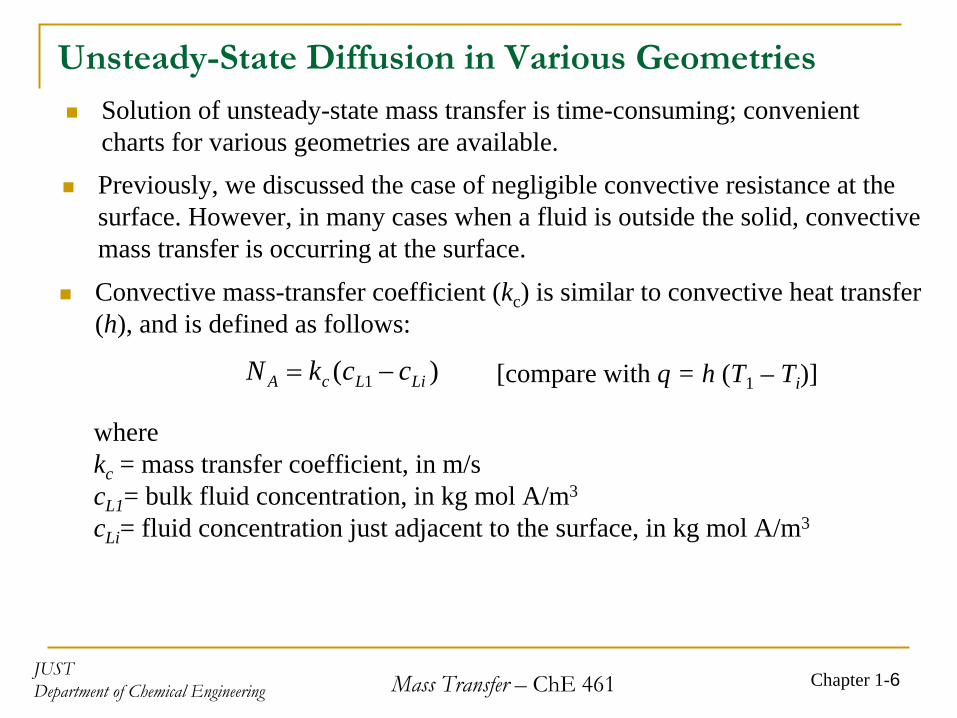
Unsteady-State Diffusion in Various GeometriesSolution of unsteady-state mass transfer is time-consuming; convenient charts for various geometries are available.Previously, we discussed the case of negligible convective resistance at the surface. However, in many cases when a fluid is outside the solid, convective mass transfer is occurring at the surface.Convective mass-transfer coefficient (kc) is similar to convective heat transfer (h), and is defined as follows:
[compare with q = h (T1 – Ti )])( 1 LiLcA cckN −=
wherekc = mass transfer coefficient, in m/scL1 = bulk fluid concentration, in kg mol A/m3
cLi = fluid concentration just adjacent to the surface, in kg mol A/m3

JUSTDepartment of Chemical Engineering Mass Transfer – ChE 461 Chapter 1-7
Different interface conditions are shown in the drawing
Concentration drop across the fluid is cL1 – cLi
The concentration of the fluid adjacent to the surface, cLi, is related to the concentration of the fluid in the solid, ci, by the following equilibrium equation:
i
Li
ccK =
K: equilibrium distribution coefficient
(similar to Henry’s law coefficient for a gas and liquid)
JUSTDepartment of Chemical Engineering Mass Transfer – ChE 461 Chapter 1-8
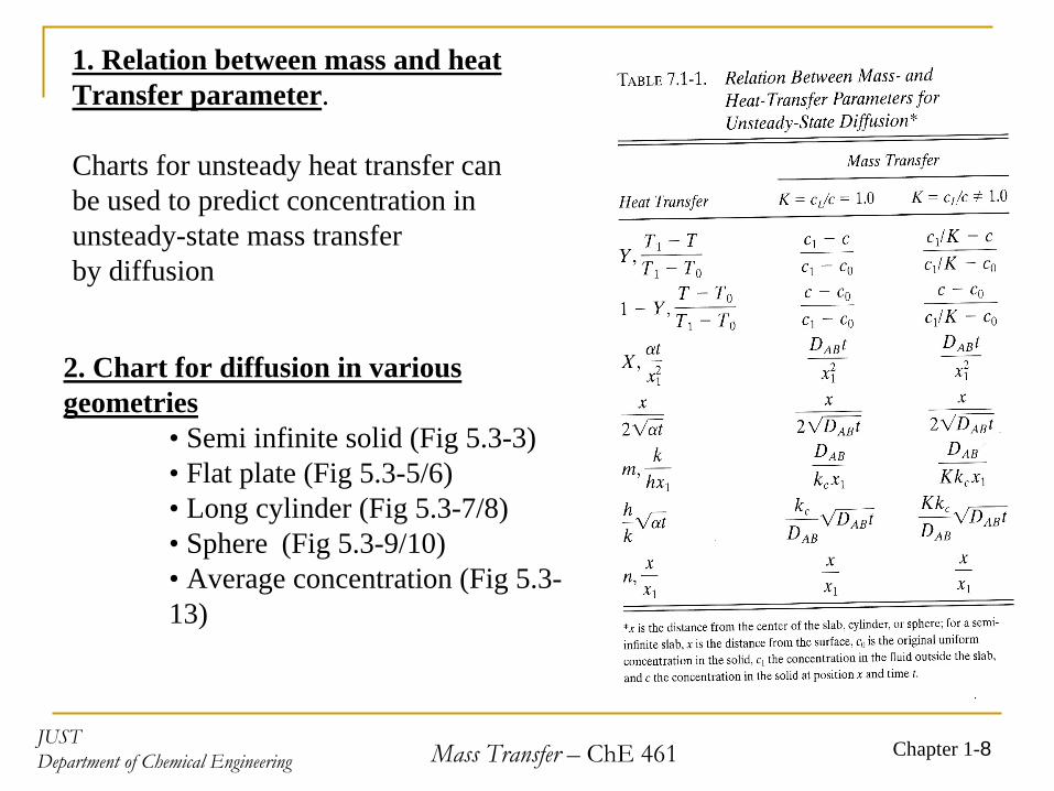
1. Relation between mass and heat Transfer parameter.
Charts for unsteady heat transfer can be used to predict concentration in unsteady-state mass transfer by diffusion
2. Chart for diffusion in various geometries
• Semi infinite solid (Fig 5.3-3)• Flat plate (Fig 5.3-5/6)• Long cylinder (Fig 5.3-7/8)• Sphere (Fig 5.3-9/10)• Average concentration (Fig 5.3- 13)

JUSTDepartment of Chemical Engineering Mass Transfer – ChE 461 Chapter 1-9
Example: Unsteady-State Diffusion in a Slab of Agar GelA solid slab of 5.15 wt% agar gel at 278 K is 10.16 mm thick and contains a uniform
concentration of urea of 0.1 kgmol/m3. Diffusion is only in the x-direction through two parallel flat surfaces 10.16 mm apart. The slab is suddenly immersed in pure turbulent water, so the surface resistance can be assumed to be negligible; that is, the convective coefficient kc is very large. The diffusivity of urea in the agar is 4.72 × 10-
10 m2/s.1) Calculate the concentration at the midpoint of the slab (5.08 mm from the surface) and
2.54 mm from the surface after 10 h.2) If the thickness of the slab is halved, what would be the midpoint concentration in 10
h?

JUSTDepartment of Chemical Engineering Mass Transfer – ChE 461 Chapter 1-10
CONVECTIVE MASS-TRANSFER COEFFICIENT
In previous chapter emphasis molecular diffusion in stagnant fluids or fluids in laminar flow. In many cases, the rate of diffusion is slow and more rapid transfer is desired.So, to achieved it the fluid velocity is increased until turbulent mass transfer occurs.
To have fluid in convective flow usually requires the fluid to be flowing past another immiscible fluid or a solid surface.Example: flowing in a pipe
Laminar flow: fluid flows in streamlines and its behavior can usually be described mathematically
Turbulent flow: no streamlines and large eddies or “chunks” of fluid exist moving rapidly in seemingly random fashion

JUSTDepartment of Chemical Engineering Mass Transfer – ChE 461 Chapter 1-11
Three regions of mass transfer can be visualized when a solute is dissolving from a solid to a fluid:
Laminar sub-layer: a thin viscous sublayer which is adjacent to the surface
• Characterized by molecular diffusion• No eddies present• Large concentration drop
Transition or buffer zone: a region adjacent to the laminar layer where gradual transition from molecular diffusion to mainly turbulent at the end occurs.
• Some eddies present• Mass transfer is the sum of turbulent + diffusion
Turbulent region: adjacent to the buffer zone where most of the transfer is by turbulent with very small diffusion
• concentration decrease very small • eddies motion
Typical plot for mass transfer of a dissolving solid from a surface to a turbulent fluid in a conduit
cA1Solid surface
Laminar sub-layer
Transition zone
Fluideddies
cA2
z
z
cA
cA1
cA2

JUSTDepartment of Chemical Engineering Mass Transfer – ChE 461 Chapter 1-12
Definition of Mass-Transfer coefficient• Previously, for molecular diffusion in stagnant fluid and fluid in laminar flow:
dzdcDJ A
ABA −=* ( )BAAA
ABA NNcc
dzdxcDN ++−=
• For turbulent flow, mass transfer is increased by eddy diffusivity, ε
(m/s)
( )dzdcDJ A
ABA ε+−=*
• ε
varied with distance, average ε
will be used; J*A1 is normally used which is
flux of A on surface area A1 (since the cress sectional area may vary) relative to the whole bulk surface.
)( 2112
*1 AA
MABA cc
zzDJ −
−+
−=ε
In terms of convective mass transfer coefficient:
12
'
zzDk MAB
c −+
=ε
)( 21'*
1 AAcA cckJ −=
where k’c is mass transfer coefficient: [Kgmol/s.m2.(kgmol/m3)]
or [m/s]

JUSTDepartment of Chemical Engineering Mass Transfer – ChE 461 Chapter 1-13
Mass-transfer coefficient for equimolar
counterdiffusion
∴ NA = -NB
( ) ( )BAAA
MABA NNcc
dzdxDcN +++−= ε
12
'
zzDk MAB
c −+
=ε
)( 21'
AAcA cckN −=
Since
where
Defining equation for the mass-transfer coefficient
• Other definitions for mass transfer coefficient depending on concentrations:
Gases: )( 21'
AAcA cckN −= )( 21'
AAG ppk −= )( 21'
AAy cyk −=Liquids: )( 21
'AAcA cckN −= )( 21
'AAL cck −= )( 21
'AAx xxk −=
• Mass transfer coefficients are related to each other, eg.
)( 21'
AAcA cckN −= )( 21'
AAy cyk −= ⎟⎠⎞
⎜⎝⎛ −=
cc
cck AA
y21'
ckk yc /'' =
( )21
'
AAy cc
ck
−=
Hence, (Also see Table 7.2-1 with corresponding units)

JUSTDepartment of Chemical Engineering Mass Transfer – ChE 461 Chapter 1-14
Mass-transfer coefficient for A diffusing through stagnant, nondiffusing
B
∴ NB = 0
12
'
zzDk MAB
c −+
=ε)( 21
'
AABM
cA cc
xkN −= where
• Rewriting using other units:Gases: )( 21 AAcA cckN −= )( 21 AAG ppk −= )( 21 AAy cyk −=Liquids: )( 21 AAcA cckN −= )( 21 AAL cck −= )( 21 AAx xxk −=
• Again, mass transfer coefficients are related to each other, eg.
( ) )(/ 21'
AABMcA ccxkN −= )( 21 AAx xxk −= ⎟⎠⎞
⎜⎝⎛ −=
cc
cck AA
x21
ckxk xBMc //' =
( )21 AAx cc
ck
−=
Hence, (Also see Table 7.2-1 with corresponding units)
)()( 21
12AA
BM
avABA xx
xzzcDN −
−=Previously, the expression was derived
With eddy diffusivity, )()(
)(21
12AA
BM
avMABA xx
xzzcDN −
−+
=ε )(
)()(
2112
AABM
MAB ccxzz
D−
−+
=ε
or
kc ≡
Mass transfer coefficient for A diffusing through stagnant B
)( 21 AAc cck −=
)( 21
'
AABM
xA xx
xkN −=or )( 21 AAx xxk −=

JUSTDepartment of Chemical Engineering Mass Transfer – ChE 461 Chapter 1-15
Example: Vaporizing A and Convective Mass TransferA large volume of pure gas B at 2 atm pressure is flowing over a surface from which
pure A is vaporizing. The liquid A completely wets the surface, which is a blotting paper. Hence, the partial pressure of A at the surface is the vapor pressure of A at 298 K, which is 0.2 atm. The k’
y has been estimated to be 6.78 × 10⁻⁵ kgmol/s.m2.mol frac. Calculate NA , the vaporization rate, and also the values of ky anf kG .

JUSTDepartment of Chemical Engineering Mass Transfer – ChE 461 Chapter 1-16
Mass Transfer Coefficient for General Case of A and B diffusing and Convective flow using Film Theory
In this case mass transfer is assumed to occur through a thin film next to the wall of thickness δf and by molecular diffusion. The experimental value of k’
c for dilute solutions is used to determine δf:
( )BAAA
ABA NNxdzdxcDN ++−=
f
ABc
Dkδ
='
( ) ( )BAAA
MABA NNcc
dzdxDcN +++−= εSince
with molecular diffusion only:
Convective term
∫∫ +−−=
=
=
2
1 )(1
0
A
A
f x
x BAAA
Az
zAB NNxNdxdz
cD
δRearranging and integration:
( )( ) ⎥
⎦
⎤⎢⎣
⎡−+−+
+=
1
2'
//ln
ABAA
ABAAc
BA
AA xNNN
xNNNckNN
NN
• when NB = 0 ( )( )21' / AABMcA ccxkN −=⇒
xA1Solid surface
Fluid
xA2
z
δf

JUSTDepartment of Chemical Engineering Mass Transfer – ChE 461 Chapter 1-17
Mass Transfer Coefficient under High Flux ConditionsThe previous case assumes that film thickness is unaffected by high flux and bulk or convective flow (diffusion-induced convection)
Other definitions of the mass transfer coefficient which includes effect of diffusion-induced convection will be derived assuming stagnant nondiffusing B
( )BAAz
AABA NNx
dzdxcDN ++⎟
⎠⎞
⎜⎝⎛−=
=0 0Defining a mass-transfer coefficient in terms of the diffusion flux,
)( 210
0AAc
z
AAB xxck
dzdxcD −=⎟
⎠⎞
⎜⎝⎛−
=
( )1
210
1 A
AAcA x
xxckN−−
=
)( 21 AAcA xxckN −=In general, kc may be defined without regard to convective flow:
(1)
(2)
cAc kxk )1( 10 −=Combining (1) and (2):
kc0 and kc → for high flux kc
’ → for low flux
JUSTDepartment of Chemical Engineering Mass Transfer – ChE 461 Chapter 1-18
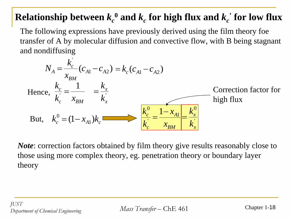
Relationship between kc0 and kc for high flux and kc
’ for low flux
)( 21
'
AABM
cA cc
xkN −=
The following expressions have previously derived using the film theory foe transfer of A by molecular diffusion and convective flow, with B being stagnant and nondiffusing
)( 21 AAc cck −=
BMc
c
xkk 1
' =Hence, 'x
x
kk
=
cAc kxk )1( 10 −=But,
BM
A
c
c
xx
kk 1
'
0 1−=
Note: correction factors obtained by film theory give results reasonably close to those using more complex theory, eg. penetration theory or boundary layer theory
'
0
x
x
kk
=
Correction factor for high flux

JUSTDepartment of Chemical Engineering Mass Transfer – ChE 461 Chapter 1-19
Example: High Flux Correction FactorsToluene A is evaporating from a wetted porous slab by having inert pure air at 1
atm flowing parallel to the flat surface. At a certain point the mass-transfer coefficient kc
’ for very low fluxes has been estimated as 0.2 lb mol/h.ft2. The gas composition at the interface at this point is xA1 = 0.65. Calculate the flux NA and the ratio kc /k’
c or kx /k’x and k0
c /k’c or k0
x /k’x to correct for high flux.

JUSTDepartment of Chemical Engineering Mass Transfer – ChE 461 Chapter 1-20
Mass-Transfer Coefficients for Various Geometries Dimensionless Numbers
μυρL
=ReReynolds number L ≡
Dp for sphereL ≡
D for pipe
L ≡
L length for plateυ: mass average velocity if in pipeυ ≡ υ’: superficial velocity in the empty cross section of a packed bed (υ = υ’/ε)
ABDρμ
=ScSchmidt number)( transfer massfor y Diffusivit
)/(y diffusivitfor component shear ABD
ρμ=
AB
c
DLk '
Sc=Sherwood numberAB
BMc
DLyk
=AB
x
DL
ck '
= = . . .
υ
'
St ck=Stanton number
M
y
Gk '
=M
G
GPk '
= = . . . GM = υρ/Mav = υc
( ) ( ) ( )1/33/2'
3/2'
Sc Re/ScSc ===M
GSc
cD G
PkNkJυ
JD factor

JUSTDepartment of Chemical Engineering Mass Transfer – ChE 461 Chapter 1-21
Analogies among Mass, Heat and Momentum transferWhy analogies?
• Similarity of molecular diffusion equation for momentum, Fourier’s for heat and Fick for mass
• Data for pressure drop and heat transfer are available more than mass transfer
• In case of turbulent flow, the differential equations will contain time average velocities and in addition the eddy diffusivities of momentum (ευ
), mass (εD ), and heat transfer (εH ). The resulting equations can not be solved for lack of information about the eddy diffusivities, but one might expect results of the form:
⎟⎟⎠
⎞⎜⎜⎝
⎛=
D
Scfεεψ υ,,
2Sc ReSh
1 ⎟⎠⎞
⎜⎝⎛=
νεψ DScf ,,
22
⎟⎟⎠
⎞⎜⎜⎝
⎛=
H
fεεψ υPr,,
2Sc ReNu
1 ⎟⎠⎞
⎜⎝⎛=
νεψ Hf Pr,,
22
• Equations or correlations for heat transfer can be used for mass transfer by replacing dimensionless number of the former by the later. See next slide
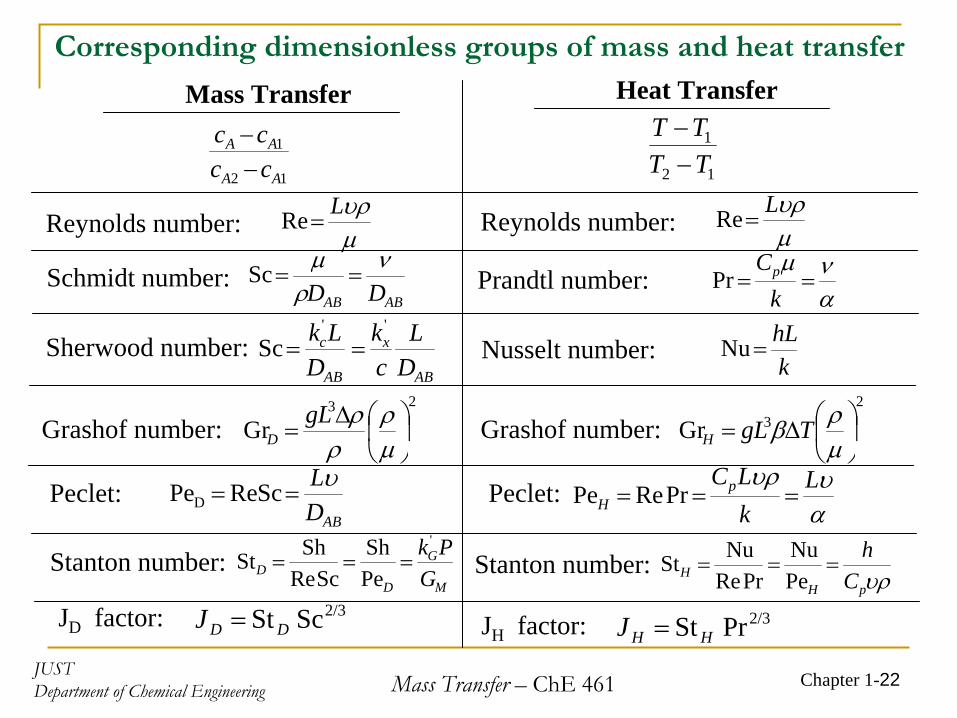
JUSTDepartment of Chemical Engineering Mass Transfer – ChE 461 Chapter 1-22
Corresponding dimensionless groups of mass and heat transfer
Mass Transfer Heat Transfer
12
1
AA
AA
cccc−−
μυρL
=Re
12
1
TTTT−−
Reynolds number: μυρL
=ReReynolds number:
ABAB DDν
ρμ
==ScSchmidt number:ανμ
==k
CpPrPrandtl number:
Sherwood number:k
hL=NuNusselt number:
AB
c
DLk '
Sc=AB
x
DL
ck '
=
Grashof number:23
Gr ⎟⎠
⎞⎜⎝
⎛Δ=
μρ
ρρgL
D Grashof number:2
3Gr ⎟⎠
⎞⎜⎝
⎛Δ=μρβ TgLH
Peclet:ABD
Lυ== ScRePeD Peclet:
αυυρ L
kLCp
H === Pr RePe
Stanton number:M
G
DD G
Pk '
PeSh
Sc ReShSt === Stanton number:
υρpHH C
h===
PeNu
Pr ReNuSt
2/3Sc St DDJ =JD factor: 2/3Pr St HHJ =JH factor:

JUSTDepartment of Chemical Engineering Mass Transfer – ChE 461 Chapter 1-23
Derivation of Mass-Transfer Coefficients in Laminar Flow
• When a fluid flowing in laminar flows and mass transfer by molecular diffusion is occurring, the equations are very similar to those for heat transfer by conduction in laminar flow.
• In theory it is not necessary to have experimental mass-transfer coefficients for laminar flow, since the equations for momentum transfer and diffusion can be solved
• Consider mass transfer of solute A into a laminar falling film as shown in the drawing
• Solute A in the gas is absorbed at the interface and then diffuses a distance into the liquid so that it does not penetrate the whole distance x = δ• Concentration profile at point z distance is shown in the drawing

JUSTDepartment of Chemical Engineering Mass Transfer – ChE 461 Chapter 1-24
0)1()1()1()1( =Δ+Δ−Δ+Δ Δ+Δ+ xNzNxNzN zzAzxxAxzAzxAx
Consider the mass balance on the elemental system:For steady-state: Rate of input = rate of output
convection zero +∂∂
−=xcDN A
ABAx
For dilute solution:
zAAz cN υ+= diffusion zero
2
2
xcD
zc A
ABA
z ∂∂
=∂∂υ
Substituting, dividing by ΔxΔz, letting ΔxΔz and approaches zero leads to:
⇒ υz is needed and has been derived in fluid mechanics: ⎥⎦
⎤⎢⎣
⎡⎟⎠⎞
⎜⎝⎛−=
2
max, 1δ
υυ xzz
Also υz,max = (3/2)υz,av
• If solute A penetrates only a short distance into the fluid: ⇒ υz = υz,max = υmax

JUSTDepartment of Chemical Engineering Mass Transfer – ChE 461 Chapter 1-25
2
2
max xcD
zc A
ABA
∂∂
=∂∂
∴υBoundary conditions:z = 0 cA = 0x = 0 cA = cA0 x = ∞
cA = 0
⎟⎟⎠
⎞⎜⎜⎝
⎛=
max0 /4erf
υzDx
cc
ABA
ASolution by Laplace transform:
00)(
== ∂
∂−=
x
AABxAx x
cDzN
Local molar flux at the surface x = 0 at position z:
zDc AB
A πυmax
0=
Total moles of A transferred per second to the liquid over the entire length:
∫ ==⋅L
xAxA dzNLN0
0)()1()1( LDcL AB
A πυmax
04)1.(=∫ ⎟
⎠⎞
⎜⎝⎛=
LAB
A dzz
Dc0 2/1
2/1max
01)1(
πυ
where L/υmax = tL ≡
time of exposure of the liquid to the solute A in the gas
∴ 5.05.0 /1 and transfermass of Rate LAB tD∝ Basis for penetration theory in turbulent mass transfer

JUSTDepartment of Chemical Engineering Mass Transfer – ChE 461 Chapter 1-26
Mass Transfer for Laminar Flow inside Pipes
• For laminar flow of a liquid or gas inside a pipe: 2100Re <=μρυD
• Experimental data for mass transfer from the wall for gases are presented graphicallycA : exit concentrationcA0 : inlet concentrationcAi : concentration at the interface between the gas and the gas
W: flow in kg/s
L: length of mass transfer section
• For liquids with small values of DAB :3/2
0
0 5.5−
⎟⎟⎠
⎞⎜⎜⎝
⎛=
−−
LDW
cccc
ABAAi
AA
ρ
JUSTDepartment of Chemical Engineering Mass Transfer – ChE 461 Chapter 1-27
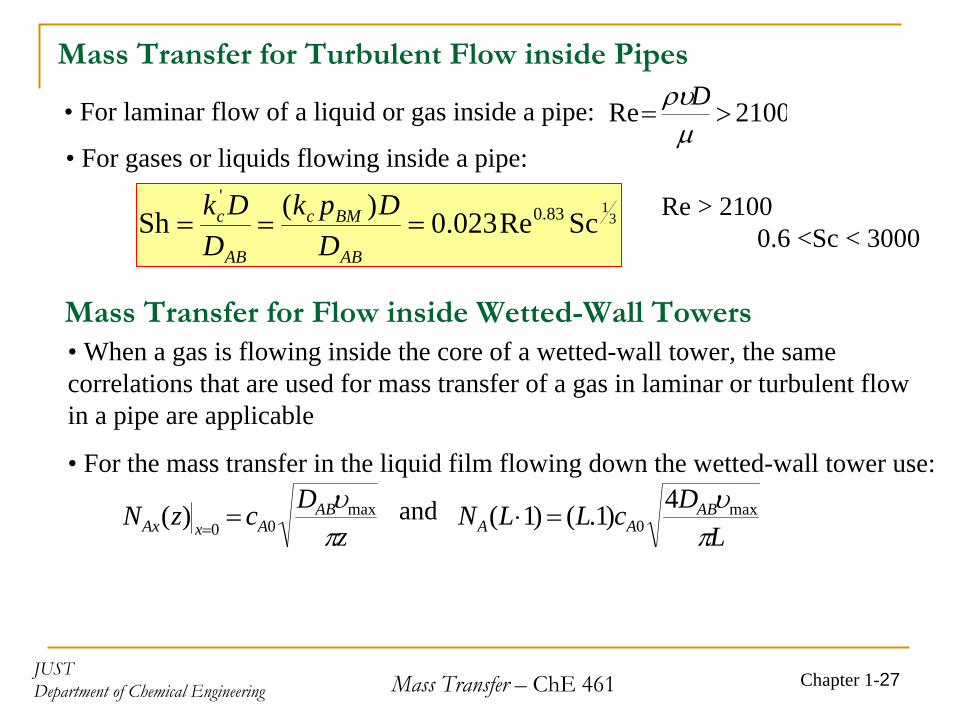
Mass Transfer for Turbulent Flow inside Pipes
• For laminar flow of a liquid or gas inside a pipe: 2100Re >=μρυD
• For gases or liquids flowing inside a pipe:
31
ScRe023.0)(Sh 83.0'
===AB
BMc
AB
c
DDpk
DDk Re > 2100
0.6 <Sc < 3000
Mass Transfer for Flow inside Wetted-Wall Towers• When a gas is flowing inside the core of a wetted-wall tower, the same correlations that are used for mass transfer of a gas in laminar or turbulent flow in a pipe are applicable
• For the mass transfer in the liquid film flowing down the wetted-wall tower use:
zDczN AB
AxAx πυmax
00)( == LDcLLN AB
AA πυmax
04)1.()1( =⋅and

JUSTDepartment of Chemical Engineering Mass Transfer – ChE 461 Chapter 1-28
Example: Mass Transfer Inside a TubeA tube is coated on the inside with naphthalene and has an inside diameter of 20 mm and a length of 1.1 m. Air at 318 K and an average pressure of 101.3 kPa flows through this pipe at a velocity of 0.8 m/s. Assuming that the absolute pressure remains essentially constant, calculate the concentration of naphthalene in the exit air.
JUSTDepartment of Chemical Engineering Mass Transfer – ChE 461 Chapter 1-29
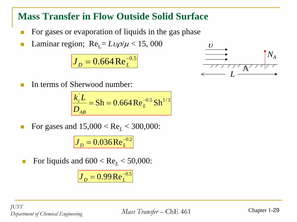
Mass Transfer in Flow Outside Solid SurfaceFor gases or evaporation of liquids in the gas phaseLaminar region; ReL= Lυρ/μ < 15, 000
In terms of Sherwood number:
5.0Re664.0 −= LDJ
3/15.0'
ShRe664.0Sh −== LAB
c
DLk
For gases and 15,000 < ReL < 300,000:2.0Re036.0 −= LDJ
For liquids and 600 < ReL < 50,000:5.0Re99.0 −= LDJ
L
NA
υ
A

JUSTDepartment of Chemical Engineering Mass Transfer – ChE 461 Chapter 1-30
Example: Mass Transfer from a Flat Plate
A large volume of pure water at 26.1oC is flowing parallel to a flat plate of solid benzoic acid, where L = 0.244 m in the direction of flow. The water velocity is 0.061 m/s. The solubility benzoic acid in water is 0.02948 kgmol/m3. The diffusivity of benzoic acid is 1.245 × 10⁻⁹ m2/s. Calculate the mass transfer coefficient kL and the flux NA .

JUSTDepartment of Chemical Engineering Mass Transfer – ChE 461 Chapter 1-31
Mass Transfer for Flow Past Single Sphere
Previously, the following equation was derived for stagnant medium
( )2112
AAp
ABA cc
DDN −=∴
⇒ Mass-transfer coefficient kc, which is k’c for a dilute solution is:
p
ABc D
Dk 2' =
Rearranging, 0.2Sh'
==AB
pc
DDk Only for very low Re= Dpυρ/μ
Gases; 0.6 < Sc < 2.7; 1 < Re = Dpυρ/μ < 48 000 3/153.0 ScRe552.00.2Sh +=
Liquids; 2 < Re = Dpυρ/μ < 2000 3/15.0 ScRe95.00.2Sh +=
Liquids; 2,000 < Re = Dpυρ/μ < 17,000 3/162.0 ScRe347.0Sh=

JUSTDepartment of Chemical Engineering Mass Transfer – ChE 461 Chapter 1-32
Example: Mass Transfer from a Sphere
Calculate the value of the mass-transfer coefficient and the flux for mass transfer from a sphere of naphthalene to air at 45oC and 1 atm flowing at a velocity of 0.305 m/s. The diameter of the sphere is 25.4 mm. The diffusivity of naphthalene in air at 45oC is 6.92×10⁻⁶ m2/s and the vapor pressure of solid naphthalene is 0.555 mm Hg.

JUSTDepartment of Chemical Engineering Mass Transfer – ChE 461 Chapter 1-33
Mass Transfer to Packed BedsTypical processing operation including packed beds
Drying operationsAdsorption or desorption of gases or liquids by solid particles, eg. charcoal Mass transfer of gases and liquids to catalyst particles
Void fraction of the bed, ε, is an important parameter in the bed:
0.2Shmin bed, theof volumeTotal
min pace, voidsof volume3
3
===ε
Gases in packed bed of spheres; 10 < Re < 10,000: 4069.0Re4548.0 −==εHD JJ
where,μυ'
Re pD=
υ’: superficial velocity (mass average velocity in the empty tube without packing
JUSTDepartment of Chemical Engineering Mass Transfer – ChE 461 Chapter 1-34
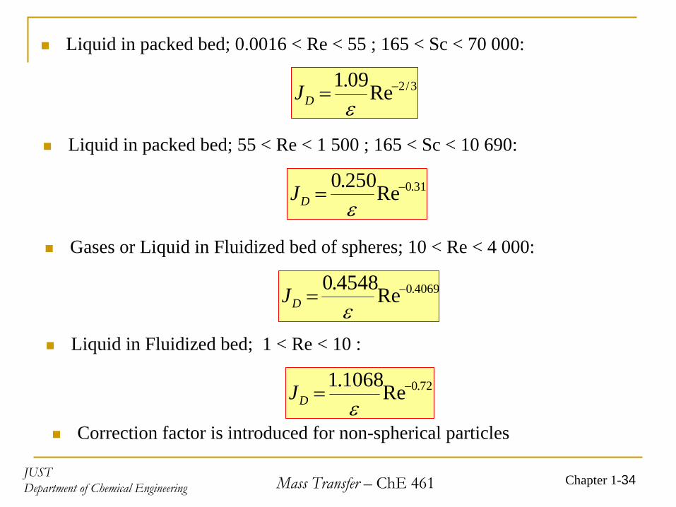
Liquid in packed bed; 0.0016 < Re < 55 ; 165 < Sc < 70 000:
3/2Re09.1 −=εDJ
Liquid in packed bed; 55 < Re < 1 500 ; 165 < Sc < 10 690:
31.0Re250.0 −=εDJ
Gases or Liquid in Fluidized bed of spheres; 10 < Re < 4 000:
4069.0Re4548.0 −=εDJ
Liquid in Fluidized bed; 1 < Re < 10 :
72.0Re1068.1 −=εDJ
Correction factor is introduced for non-spherical particles

JUSTDepartment of Chemical Engineering Mass Transfer – ChE 461 Chapter 1-35
Calculation Method for Packed BedsSelect proper correlation for JD and then calculate kc in m/s. Calculate the total external surface area A m2 of the solids
bp
b VD
aVA )1(6 ε−==
)]/()ln[()()(
21
21
AAiAAi
AAiAAicA cccc
ccccAkAN−−−−−
=
a: m2 surface area/m3 total volumeVb : total volume of the bed, in m3
Calculate the log mean driving force at the inlet and outlet of the bed:
cAi : concentration at the surface of the solid, kg mol/m3;cA1 : inlet bulk fluid concentration, kg mol/m3;cA2 : outlet bulk fluid concentration, kg mol/m3;

JUSTDepartment of Chemical Engineering Mass Transfer – ChE 461 Chapter 1-36
Example: Mass Transfer of a Liquid in a Packed BedPure water at 26.1oC flows at the rate of 5.514×10⁻⁷ m3/s through a packed bed of benzoic-
acid spheres having a diameter of 6.375 mm. The total surface area of the spheres in the bed is 0.01198 m2 and the void fraction is 0.436. The tower diameter is 0.0667 m. The solubility of benzoic acid in water is 2.948×10⁻² kg mol/m3.
1. Predict the mass-transfer coefficient kc . Compare with the experimental value of 4.665×10⁻⁶ m/s.
2. Using the experimental value of kc , predict the outlet concentration of benzoic acid in the water

JUSTDepartment of Chemical Engineering Mass Transfer – ChE 461 Chapter 1-37
Mass Transfer to Suspensions of Small Particles
ExamplesLiquid-liquid hydrogenation -hydrogen diffuse from gas bubbles through an
organic liquid then to small suspended catalyst particles.Fermentation-oxygen diffuses from small gas bubbles through the aqueous
medium then to the small suspended particles.
1. Mass Transfer to small particles <0.6 mmTo predicts mass transfer coefficients from small gas bubbles such as oxygen or air to the liquid phasefrom liquid phase to the surface of small catalyst particles, microorganisms, solids or liquids.
31
23/2Sc31.02' ⎟⎟
⎠
⎞⎜⎜⎝
⎛ Δ+= −
c
c
P
ABL p
gDDk ρμ Δρ = ρc - ρp
ρc : density of continuous phaseMolecular diffusion Due to free fall or rise of the sphere due to gravitation

JUSTDepartment of Chemical Engineering Mass Transfer – ChE 461 Chapter 1-38
Example: Mass Transfer from Air Bubbles in Fermentation
Calculate the maximum rate of absorption of O2 in a fermenter from air bubbles at 1 atm pressure having diameters of 100 μm at 37oC into water having a zero concentration of dissolved O2 . The solubility of O2 from air in water at 37oC is 2.26×10⁻⁷ g mol O2 /cm3 liquid or 2.26×10⁻⁴ kg mol O2 /m3. The diffusivity of O2 in water at 37oC is 3.25×10⁻⁹ m2/s. Agitation is used to produce the air bubbles.
JUSTDepartment of Chemical Engineering Mass Transfer – ChE 461 Chapter 1-39
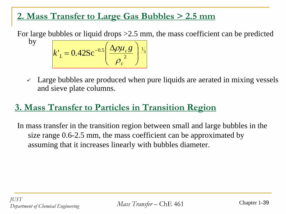
2. Mass Transfer to Large Gas Bubbles > 2.5 mm
For large bubbles or liquid drops >2.5 mm, the mass coefficient can be predicted by
Large bubbles are produced when pure liquids are aerated in mixing vessels and sieve plate columns.
31
25.0Sc42.0' ⎟⎟
⎠
⎞⎜⎜⎝
⎛ Δ= −
c
cL
gkρρμ
3. Mass Transfer to Particles in Transition Region
In mass transfer in the transition region between small and large bubbles in the size range 0.6-2.5 mm, the mass coefficient can be approximated by assuming that it increases linearly with bubbles diameter.

JUSTDepartment of Chemical Engineering Mass Transfer – ChE 461 Chapter 1-40
4. Mass Transfer to Particles in Highly Turbulent Mixers
When agitation power is increased beyond that needed for suspension of solid or liquids particles and the turbulence force become larger than the gravitational forces, so mass transfer coefficient
( )4
1
23/2 /13.0Sc' ⎟⎟
⎠
⎞⎜⎜⎝
⎛=
c
cL
gVPkρ
μ P/V: power input per unit volume

JUSTDepartment of Chemical Engineering Mass Transfer – ChE 461 Chapter 1-41
Molecular Diffusion Plus Convection and Chemical Reaction
J*A: molar flux of A in kg mol A/s.m2 relative to molar average velocity υM
NA: molar flux of A relative to stationary coordinate
AAA υρ=n (kg A/s.m2) AAA υcN = (kg mol A/s.m2) or
Assuming υ to be the mass average velocity of the stream relative to stationary coordinate and can be obtained from υA and υB as:
AA υυυ AA ww +=
where wA = ρA /ρ (weight fraction of A)
υA : velocity of A relative to stationary coordinate
BA υυυ BAM xx +=
Molar average velocity υM in m/s relative to stationary coordinate is:
BA υυcc
cc BA +=
BA υρρυ
ρρ BA +=
JUSTDepartment of Chemical Engineering Mass Transfer – ChE 461 Chapter 1-42
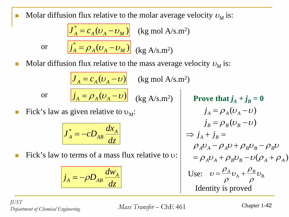
Molar diffusion flux relative to the molar average velocity υM is:
)(*MAAA cJ υυ −= (kg mol A/s.m2)
)(*MAAAj υυρ −= (kg A/s.m2)or
Molar diffusion flux relative to the mass average velocity υM is:
)( υυ −= AAA cJ (kg mol A/s.m2)
)( υυρ −= AAAj (kg A/s.m2)or
Fick’s law as given relative to υM:
dzdxcDJ A
ABA −=*
Fick’s law to terms of a mass flux relative to υ:
dzdwDj A
ABA ρ−=
Prove that jA + jB = 0
)( υυρ −= BBBj)( υυρ −= AAAj
=+⇒ BA jjυρυρυρυρ BBBAAA −+−
)( AABBAA ρρυυρυρ +−+=
BA υρρυ
ρρυ BA +=Use:
Identity is proved

JUSTDepartment of Chemical Engineering Mass Transfer – ChE 461 Chapter 1-43
Equation of Continuity for a Binary MixtureObjective: Derive general equation for a binary mixture of A and B for diffusion
and convection including unsteady state diffusion and chemical reaction
Consider the element ΔxΔyΔx fixed in spaceGeneral mass balance on A is:
⎟⎠
⎞⎜⎝
⎛=⎟
⎠
⎞⎜⎝
⎛
+⎟⎠
⎞⎜⎝
⎛−⎟
⎠
⎞⎜⎝
⎛
onaccumulatiof rate
A mass of generationof rate
outA massof rate
inA massof rate
dtdmzyxr
yxnzxnzynyxnzxnzyn
A
zzAzyyAyxxAxzAzyAyxAx
=ΔΔΔ+
ΔΔ−ΔΔ−ΔΔ−ΔΔ+ΔΔ+ΔΔ Δ+Δ+Δ+
nAz⏐z
Δx
Δy
ΔznAx⏐x nAx⏐x+Δx
x
z
y
nAz⏐z+Δz
Divide by ΔxΔyΔz and letting ΔxΔyΔz approach zero:

JUSTDepartment of Chemical Engineering Mass Transfer – ChE 461 Chapter 1-44
AAzAyAxA rz
ny
nx
nt
=⎟⎟⎠
⎞⎜⎜⎝
⎛∂∂
+∂∂
+∂∂
+∂∂ρ
In vector notation: ( ) AAA rn
t=⋅∇+
∂∂ρ
AAzAyAxA Rz
Ny
Nx
Nt
c=⎟⎟
⎠
⎞⎜⎜⎝
⎛∂∂
+∂∂
+∂∂
+∂∂
Dividing both sides by MA :
RA : kmol A/s.m3
Substituting NA and Fick’s law from:MA
AABAz c
dzdxcDN υ+−=
( ) ( ) AAABMAA RxcDct
c=∇⋅∇−⋅∇+
∂∂ υ Final General equation

JUSTDepartment of Chemical Engineering Mass Transfer – ChE 461 Chapter 1-45
Equation for constant c and DAB
:
( ) ( ) ( ) AAABAMMAA RcDcct
c=∇−⋅∇+⋅∇+
∂∂ 2υυ
Equimolar
counterdiffusion
for gases:
dzdcDN A
ABAz −= (or υM = 0)
Assuming DAB = constant and RA = 0
⎟⎟⎠
⎞⎜⎜⎝
⎛∂∂
+∂∂
+∂∂
=∂∂
2
2
2
2
2
2
zc
yc
xcD
tc AAA
ABA (previously derived)

JUSTDepartment of Chemical Engineering Mass Transfer – ChE 461 Chapter 1-46
Diffusion and Chemical Reaction at the Boundary
Consider gas A diffusing from the bulk gas phase to the catalyst surface, where it reacts instantaneously and reversibly as follows:
A → 2BGas B then diffuses back, see the drawing δ
zz1 z2
NANB
catalystsurface
At steady state, NA = - 2NB
)( BAAA
ABAz NNxdzdxcDN ++−=Since,
)2( BAAA
ABAz NNxdzdxcDN −+−=
Rearranging and integration, ∫∫ +−=
=
=
2
1
2
1 10
A
A
x
x A
AAB
z
zA x
dxcDdzNδ
or,2
1
11ln
A
AABA x
xcDN++
=δ
Instantaneous ⇒ xA2 = 0
JUSTDepartment of Chemical Engineering Mass Transfer – ChE 461 Chapter 1-47
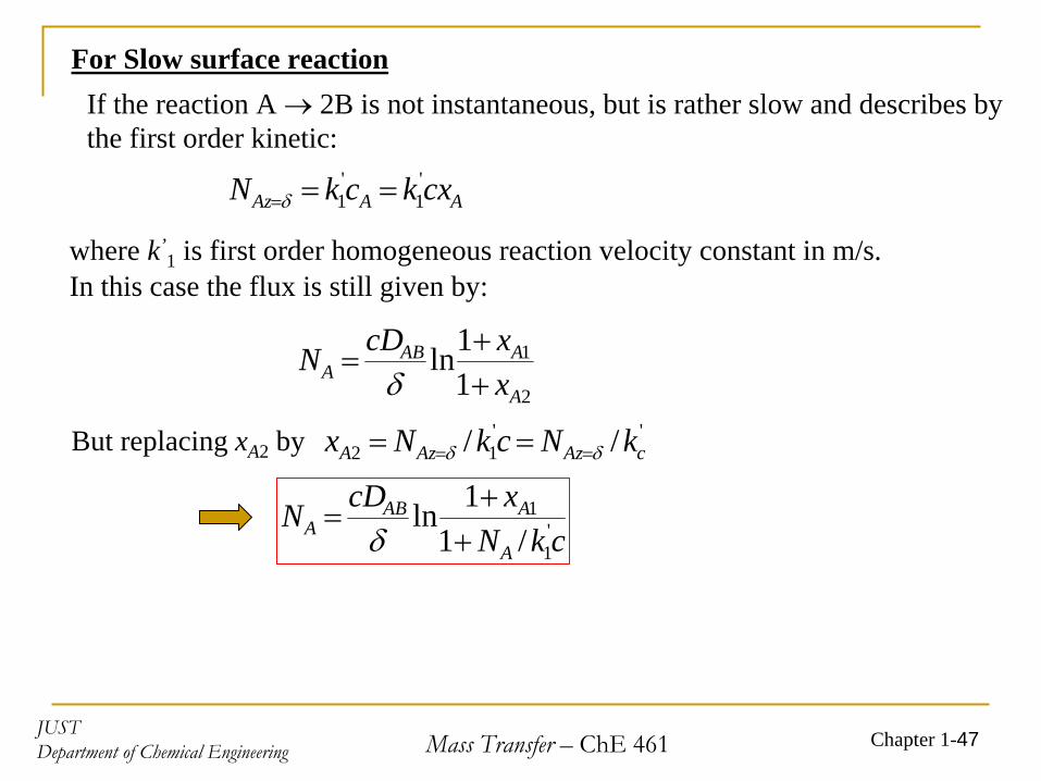
For Slow surface reaction
2
1
11ln
A
AABA x
xcDN++
=δ
If the reaction A → 2B is not instantaneous, but is rather slow and describes by the first order kinetic:
AAAz cxkckN '1
'1 ===δ
''12 // cAzAzA kNckNx δδ == ==
where k’1 is first order homogeneous reaction velocity constant in m/s.
In this case the flux is still given by:
But replacing xA2 by
ckNxcDNA
AABA '
1
1
/11ln++
=δ
JUSTDepartment of Chemical Engineering Mass Transfer – ChE 461 Chapter 1-48
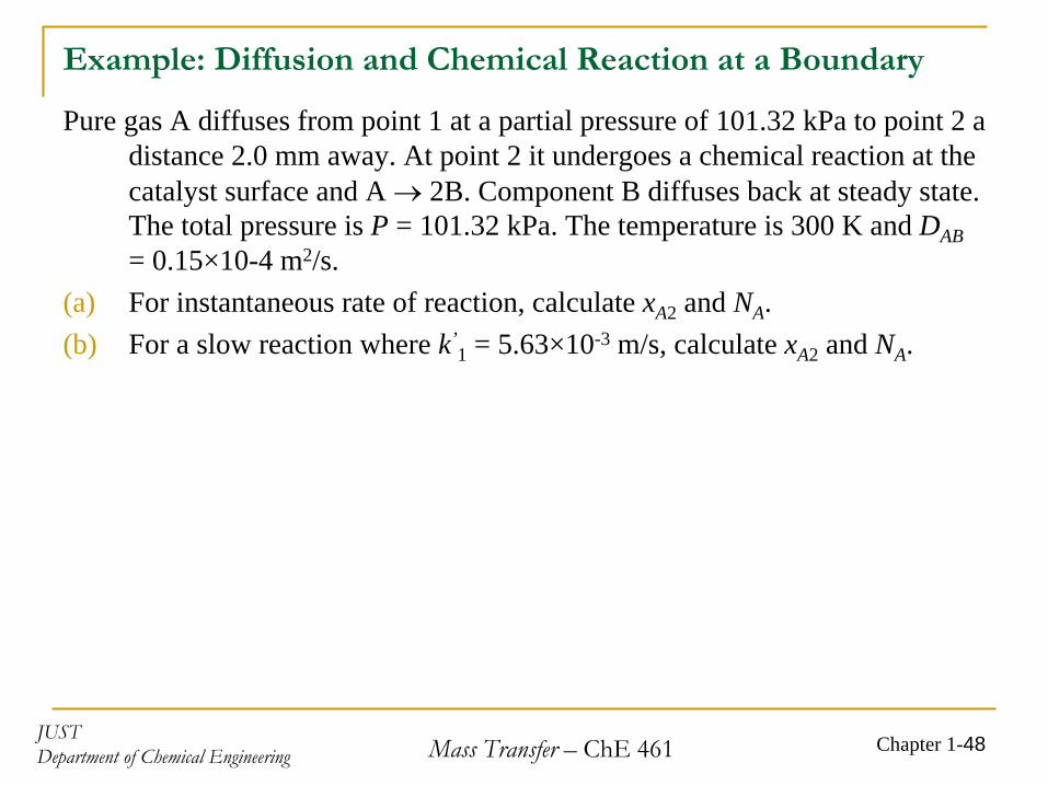
Example: Diffusion and Chemical Reaction at a Boundary
Pure gas A diffuses from point 1 at a partial pressure of 101.32 kPa to point 2 a distance 2.0 mm away. At point 2 it undergoes a chemical reaction at the catalyst surface and A → 2B. Component B diffuses back at steady state. The total pressure is P = 101.32 kPa. The temperature is 300 K and DAB = 0.15×10⁻⁴ m2/s.
(a) For instantaneous rate of reaction, calculate xA2 and NA .(b) For a slow reaction where k’
1 = 5.63×10⁻³ m/s, calculate xA2 and NA .
JUSTDepartment of Chemical Engineering Mass Transfer – ChE 461 Chapter 1-49
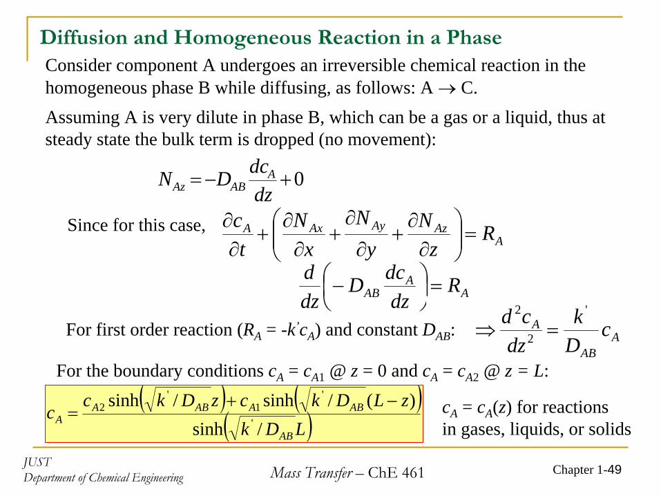
Diffusion and Homogeneous Reaction in a Phase
AAzAyAxA Rz
Ny
Nx
Nt
c=⎟⎟
⎠
⎞⎜⎜⎝
⎛∂∂
+∂∂
+∂∂
+∂∂
Consider component A undergoes an irreversible chemical reaction in the homogeneous phase B while diffusing, as follows: A → C.
0+−=dzdcDN A
ABAz
Assuming A is very dilute in phase B, which can be a gas or a liquid, thus at steady state the bulk term is dropped (no movement):
Since for this case,
AA
AB Rdz
dcDdzd
=⎟⎠⎞
⎜⎝⎛−
For first order reaction (RA = -k’cA ) and constant DAB : AAB
A cDk
dzcd '
2
2
=⇒
For the boundary conditions cA = cA1 @ z = 0 and cA = cA2 @ z = L:( ) ( )
( )LDkzLDkczDkc
cAB
ABAABAA /sinh
)(/sinh/sinh'
'1
'2 −+
= cA = cA (z) for reactionsin gases, liquids, or solids
JUSTDepartment of Chemical Engineering Mass Transfer – ChE 461 Chapter 1-50
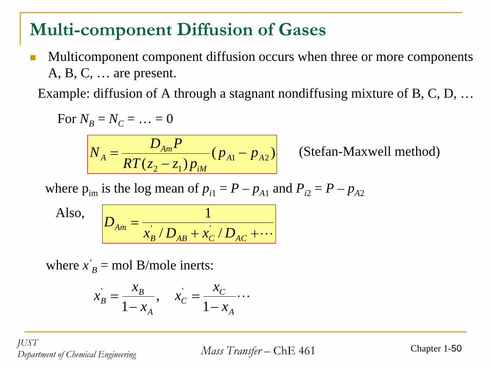
Multi-component Diffusion of GasesMulticomponent component diffusion occurs when three or more components A, B, C, … are present.
Example: diffusion of A through a stagnant nondiffusing mixture of B, C, D, …
For NB = NC = … = 0
)()( 21
12AA
iM
AmA pp
pzzRTPDN −
−= (Stefan-Maxwell method)
where pim is the log mean of pi1 = P – pA1 and Pi2 = P – pA2
Also,⋅⋅⋅++
=ACCABB
Am DxDxD
//1
''
where x’B = mol B/mole inerts:
,1
'
A
BB x
xx−
= ⋅⋅⋅−
=A
CC x
xx1
'

JUSTDepartment of Chemical Engineering Mass Transfer – ChE 461 Chapter 1-51
Example: Diffusion of A Through Nondiffusing
B and CAt 298 K and 1 atm total pressure, methane (A) is diffusing at steady state
through nondiffusing argon (B) and helium (C), At z = 0, the partial pressures in atm are pA1 = 0.4, pB1 = 0.4, and pC1 = 0.2, and at z2 = 0.005 m, pA2 = 0.1, pB2 = 0.6, and pC2 = 0.3. The binary diffusivities from Table 6.2-1 are DAB = 2.02×10⁻⁵ m2 /s, DAC = 6.75×10⁻⁵ m2 /s, DBC = 7.29×10⁻⁵ m2 /s. Calculate NA .


![Chapter 2 [Chapter 2]](https://static.fdocuments.in/doc/165x107/61f62040249b214bf02f4b97/chapter-2-chapter-2.jpg)