CHAPTER 18 Power curves for wind turbines...The more complex shape of a real wind turbine cer-tainly...

CHAPTER 18

Power curves for wind turbines

Patrick Milan , Matthias Wächter , Stephan Barth & Joachim Peinke ForWind Center for Wind Energy Research of the Universities of Oldenburg, Bremen and Hannover, Oldenburg, Germany.

The concept of a power curve is introduced, as well as the principles of the power conversion performed by a wind turbine. As an appropriate approach for the estimation of the annual power production of a wind turbine, the procedure to determine the power curve after the international standard IEC 61400 of the Inter-national Electrotechnical Commission (IEC) is discussed. As another approach is introduced a stochastic defi nition of a power curve which is based on high fre-quency measurement data and on the dynamic response of the wind turbine to wind fl uctuations. The latter approach should be seen as a completion to the IEC defi nition which provides further insight into the dynamic performance of a wind turbine and may be used as a monitoring tool for wind turbines.

1 Introduction

The overall purpose of a wind turbine is to produce electrical power from wind. Quantifying this power output is necessary, on the one hand, for the fi nancial plan-ning of any wind energy project. On the other hand, besides the pure amount of energy production, also the dynamics of the power conversion contains essential information about, e.g. mechanical and electrical performance of the turbine and power quality. Following the turbulent behavior of the wind, the power produc-tion of a wind turbine fl uctuates on short-time scales [ 1 ]. While exploiting the free, uncontrolled input that is the wind, it is of primary importance to control the stability of the power output of wind turbines. A large integration into energy networks supposes a good command of the power production, in terms of quantity, quality and availability.

To achieve such control, it is necessary to understand the behavior of wind turbines and quantify it. This is the scope of power performance techniques. This chapter

www.witpress.com, ISSN 1755-8336 (on-line) WIT Transactions on State of the Art in Science and Engineering, Vol 44, © 2010 WIT Press

doi:10.2495/978-1-84564- /205-1 18

596 Wind Power Generation and Wind Turbine Design

introduces such methods, so as to estimate the performance of a wind turbine. The procedure applies to single wind turbines, while ongoing developments lead towards integration of entire wind parks, and possibly large networks.

The approach is restricted to large-scale horizontal-axis wind turbines here. It is also assumed that the produced electrical energy is directly fed into the grid. This is not an essential restriction but facilitates putting the presented work in a relevant context. For a detailed overview of different types of wind turbines and corresponding modes of operation see, e.g. [ 2 ].

2 P ower performance of wind turbines

2.1 Introduction to power performance

In the past 30 years, recommendations and standards were defi ned to determine the power performance of a wind turbine. Permanently developed, the International Electrotechnical Commission (IEC) set the international standard IEC 61400-12 and its revised version IEC 61400-12-1 in 2005 [ 3 ]. These common guidelines defi ned the power performance characteristic of a wind turbine by the so-called power curve and its corresponding estimated annual energy production (AEP). The IEC standard gives a good estimation of long-time power production (through the AEP), which is of primary importance for an economical approach to wind energy.

Regarding actual power performance, the power curve is a powerful tool to estimate the power extraction process, as it quantifi es the relation between incom-ing wind and power output of a wind turbine. Simultaneous measurements of wind speed u ( t ) and power output P ( t ) must be performed for the wind turbine con-cerned. Here the power output P ( t ) is the net power released by the wind turbine into the electrical grid. From this data collection, a functional relation P ( u ) can be defi ned, and a two-dimensional curve of power output vs. incoming wind speed can be derived. This is what power performance refers to. Such procedure can then be applied on single wind turbines in order to characterize their power performance, monitor their behavior over time as well as predict their power production. While this prediction is well described by the IEC defi nition of AEP, monitoring methods can be defi ned based on a dynamical approach to wind energy conversion.

In order to test power performance, a measurement of the wind velocity must be performed. As a wind turbine distorts the incoming wind fi eld, a measurement in the rotor plane or closeby is not useful, at least not without further corrections. Instead the incoming upstream velocity is generally chosen as representative of the wind fi eld, and measured from a meteorological mast at turbine hub height, a cer-tain distance in front of the turbine. Based on these considerations, it becomes possible to quantify the power performance of a wind turbine in simple ways.

2.2 Theoretical considerations

The purpose of this section is to give a simple understanding of fl uid mechanics applied to wind turbines. A detailed description of the formulas and derivations


Power Curves for Wind Turbines 597

presented here can be found in [ 2 ]. This theoretical approach sets ground for the further power curve analysis.

In the following derivation, the complexity of turbulence will be set aside so as to understand the fundamental behavior of a wind turbine. Atmospheric wind has fi nite time and space structures, more commonly referred to as turbulent struc-tures. Its statistics display complex properties like unstationarity or intermittency (such as gusts), whose effects will not be discussed in this section. They repre-sent active research topics whose detailed analysis is outside the scope of this introduction, cf. [ 4 ]. In this section, a uniform fl ow at steady-state is considered.

Based on the fact that a wind turbine converts the wind power into available electrical power, one can assume the following relation:

p wind( ) ( ) ( )P u c u P u= (1)

where P wind ( u ) is the power contained in the wind passing with speed u through the wind turbine, and P ( u ) is the electrical power extracted. The power coeffi cient c p ( u ) represents the amount of power converted by the wind turbine. Because the input P wind ( u ) cannot be controlled, improvements in wind power performance involve increasing the power coeffi cient c p ( u ). Momentum theory can now be applied to determine this coeffi cient.

Consider a volume of air moving towards the wind turbine, which is modeled as an actuator disc of diameter D . A stream-tube is defi ned here as the volume of air that interacts with the turbine (see Fig. 1 ). The wind is affected by the wind turbine when crossing its swept area as the turbine extracts part of its energy. The extrac-tion of kinetic energy accounts for a drop in the wind speed from upstream to downstream, as shown in Fig. 1 . To ensure mass conservation, the stream-tube has to expand in area downstream, as shown in Fig. 1 [ 2 ].

Following this simple analysis, one can estimate the amount of kinetic energy available for extraction. The wind power P wind ( u ) is derived from momentum theory for the wind passing with speed u through the rotor of area p D ²/4:

Figure 1 : A visual representation of an airfl ow on a wind turbine. The stream-tube is affected by the presence of the wind turbine that extracts part of its energy.



23

wind ( )2 4

DP u u

r p= ( 2)

where r is the air density. This stream-tube expansion shows that c p ( u ) has a physical limit called Betz

limit such that c p ( u ) ≤ 16/27 ≈ 0.593 [ 2 , 5 ]. Regardless of its design, a wind turbine can thus extract at most 59.3% of the wind energy. Figure 2 shows the power coef-fi cient as a function of a = (1 − u downstream / u upstream ), the axial fl ow induction factor a gives the ratio of speed lost by the wind. The Betz limit corresponds to the maximum power a wind turbine can extract, when a = 1/3 [ 2 ]. This result is obtained for an actuator disc. The more complex shape of a real wind turbine cer-tainly brings a lower limit for c p . This physical limit is due to the stream-tube expansion induced by the presence of the turbine, i.e. by distorting the wind fi eld, a wind turbine sets a limit for the energy availability. Criticism of this approach is given in [ 6 , 7 ], leading to a less well defi ned upper limit of c p .

Although it is based on a simplifi ed approach, the Betz limit is a widely used and accepted value. The power coeffi cients of modern commercial wind turbines reach values of 0.45 and more. Physical aspects that limit the value of the power coeffi cient are, e.g. the fi nite number of blades and losses due to the drag and stall effects of the blades [ 2 , 8 ].

Joining eqns ( 1 ) and ( 2 ), the theoretical power curve reads

23

theoretical p wind p( ) ( ) ( ) ( )2 4

DP u c u P u c u u

r p= =

(3 )

P theoretical ( u ), or more simply P ( u ) is the electrical power output and u is the input wind speed ( u upstream ), i.e. a power curve is roughly characterized by a cubic

Figure 2: Power coeffi cient c p as a function of the axial fl ow induction factor a .



increase of the power output with the wind speed. The functional behavior of the power coeffi cient c p ( u ) is the result of certain control strategies as well as of Betz physical limit.

In the mechanical power extraction the usual way to control power production is achieved by stall effects on the rotor blades. Stall effects happen when the criti-cal angle of attack for an airfoil is exceeded, resulting in a sudden reduction in the lift forces generated by the airfoil. In modern wind turbines this is achieved by so-called active stall control or pitch control [ 2 ]. This consists of a rotation of the blades into the plane of rotation and the blade cross-section. The blade rotation angle is known as blade pitch angle q . The power coeffi cient c p is in this case a function of the blade pitch angle q and the tip-speed ratio l = w R / u (where w is the angular velocity of the rotor, R the rotor radius, i.e. blade length and u the wind speed), i.e. c p = c p [ l ( u ), q ]. Thus, the power extraction of wind turbines is opti-mized via c p [ l ( u ), q ] to a desired power production. In particular for high wind conditions c p is lowered to protect the turbine machinery and avoid overshoots in power production.

To achieve an effi cient pitch control during wind energy conversion the wind turbine is equipped by a power controller system. This is generally com-posed of several composite mechanical–electrical components that, depending on the type of design, operate actively for the optimum power performance. As a consequence the power output operation for active stall wind turbine systems can be separated into two states: partial load, with maximum c p value, and full load, with reduced c p values. A complete detail of the overall structure of the power operation system for different wind turbine types is described in [ 2 ]. Numerical wind turbine simulation can be found, e.g. in [ 9 ]. The theo-retical power curve P ( u ) together with the corresponding c p ( u ) is represented in Fig. 3 .

Figure 3 : LEFT: Static (steady-state) power curve P ( u ) of an active stall controlled wind turbine showing the different power operation states: stop, partial and full load. RIGHT: Corresponding power coeffi cient c p ( u ).



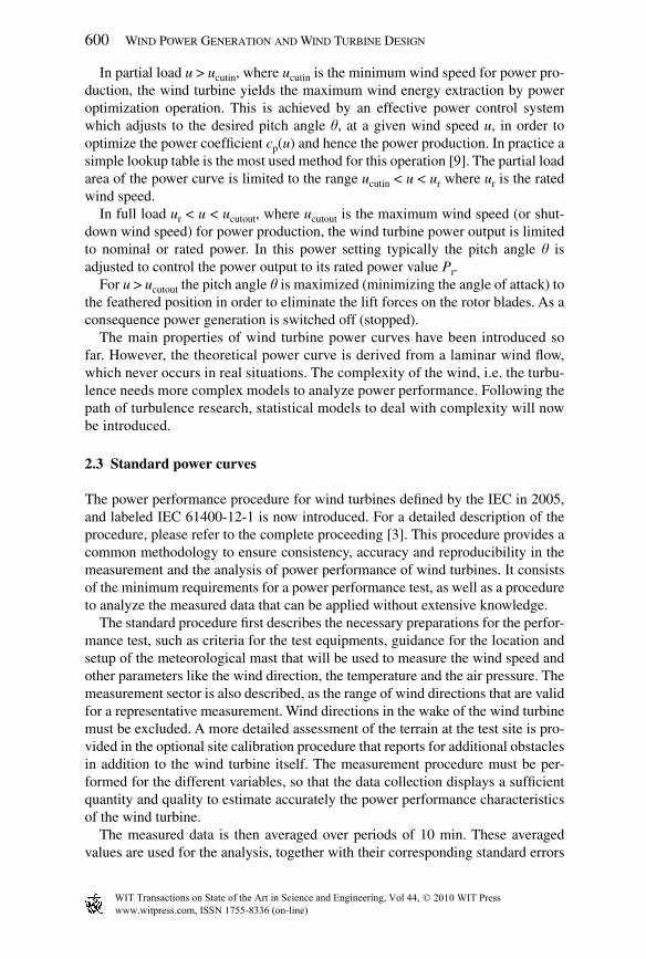
In partial load u > u cutin , where u cutin is the minimum wind speed for power pro-duction, the wind turbine yields the maximum wind energy extraction by power optimization operation. This is achieved by an effective power control system which adjusts to the desired pitch angle q , at a given wind speed u , in order to optimize the power coeffi cient c p ( u ) and hence the power production. In practice a simple lookup table is the most used method for this operation [ 9 ]. The partial load area of the power curve is limited to the range u cutin < u < u r where u r is the rated wind speed.

In full load u r < u < u cutout , where u cutout is the maximum wind speed (or shut-down wind speed) for power production, the wind turbine power output is limited to nominal or rated power. In this power setting typically the pitch angle q is adjusted to control the power output to its rated power value P r .

For u > u cutout the pitch angle q is maximized (minimizing the angle of attack) to the feathered position in order to eliminate the lift forces on the rotor blades. As a consequence power generation is switched off (stopped).

The main properties of wind turbine power curves have been introduced so far. However, the theoretical power curve is derived from a laminar wind fl ow, which never occurs in real situations. The complexity of the wind, i.e. the turbu-lence needs more complex models to analyze power performance. Following the path of turbulence research, statistical models to deal with complexity will now be introduced.

2.3 Standard power curves

The power performance procedure for wind turbines defi ned by the IEC in 2005, and labeled IEC 61400-12-1 is now introduced. For a detailed description of the procedure, please refer to the complete proceeding [ 3 ]. This procedure provides a common methodology to ensure consistency, accuracy and reproducibility in the measurement and the analysis of power performance of wind turbines. It consists of the minimum requirements for a power performance test, as well as a procedure to analyze the measured data that can be applied without extensive knowledge.

The standard procedure fi rst describes the necessary preparations for the perfor-mance test, such as criteria for the test equipments, guidance for the location and setup of the meteorological mast that will be used to measure the wind speed and other parameters like the wind direction, the temperature and the air pressure. The measurement sector is also described, as the range of wind directions that are valid for a representative measurement. Wind directions in the wake of the wind turbine must be excluded. A more detailed assessment of the terrain at the test site is pro-vided in the optional site calibration procedure that reports for additional obstacles in addition to the wind turbine itself. The measurement procedure must be per-formed for the different variables, so that the data collection displays a suffi cient quantity and quality to estimate accurately the power performance characteristics of the wind turbine.

The measured data is then averaged over periods of 10 min. These averaged values are used for the analysis, together with their corresponding standard errors



(based on the standard deviations). A normalization must then be applied to the measurement data. Depending on the type of turbine, either the means of wind speed (for turbines with active power control) or of power output (for stall-regulated turbines) must be normalized to a reference air density.

The IEC power curve is then derived from the normalized values using the so-called method of bins, i.e. the data is split into wind speed intervals of a width of 0.5 m/s each. For each interval i , bin averages of wind speed u i and power output P i are calculated according to

norm, , norm, ,

1 1

1 1and

i iN N

i i j i i ji ii i

u u P PN N= =

= =∑ ∑ ( 4)

where u norm, i , j and P norm, i , j are the normalized values of wind speed and power aver-aged over 10 min, and N i is the number of 10 min data sets in the i th bin.

For the power curve to be complete, or reliable, each bin must include at least 30 min of sampled data and the entire measurement must cover a minimum period of 180 h of data sampling. The range of wind speeds shall extend from 1 m/s below cutin wind speed to 1.5 times the wind speed at 85% of the rated power P r of the wind turbine. Such power curve was represented in Fig. 4 for a multi-MW wind turbine. Error bars were included following the recommendations below.

The standard also provides a description of the evaluation of uncertainty in the power performance measurement [ 3 ]. In a fi rst step, the respective uncertainties are obtained from the measurement as the standard error of the normalized power data. Additional uncertainties are related to the instruments, the data acquisition system and the surrounding terrain.

Figure 4 : Power curve (line) obtained from the IEC standard procedure for a multi-MW wind turbine. Corresponding error bars were displayed. The grey dots represent 10-min averages. The power output is normalized by its rated value P r .



Based on the IEC procedure, the AEP can be derived by integrating the mea-sured power curve to a reference distribution of wind speed for the test site, assum-ing a given availability of the wind turbine [ 3 ]. The AEP is a central feature for economical considerations.

The standard procedure defi ned by the IEC offers some interesting insights. It is a great advance as it sets a common ground for wind power performance. As the wind industry develops, common standards help building a general understanding between manufacturers, scientists and end-users. The IEC procedure serves this purpose as the most widely used method to estimate power performance.

A detailed analysis of this standard is of great importance for anyone who wishes to test power performance. The procedure defi nes a set of important param-eters, such as the wind direction, terrain corrections and requirements for wind speed measurements. These parameters are relevant for performance measure-ments, regardless of the fi nal method used to handle data. The main strength of the method lies in the defi nition of these important parameters.

Unfortunately, the standard procedure presents important limits. In contrast to a good defi nition of the requirements above, the way the measured data is analyzed suffers mathematical imperfections. In order to deal with the complexity of the conversion process, the data is systematically averaged. A statistical averaging is indeed necessary to extract the main features of the complex process, and the cen-tral question is how to perform this averaging. The IEC method applies the averag-ing over 10-min intervals, which lack physical meaning. The wind fl uctuates on various time scales, down to seconds (and less). A systematic averaging over such time scales as 10 min neglects all high frequency fl uctuations present in the wind dynamics, but also in the dynamics of the extraction process. In combination with the fundamental non-linearity characteristics of the power curve, i.e. P ( u ) ∝ u 3 , the resulting power curve is spoiled by mathematical errors, as derived below [see eqn ( 7 )].

One can split the wind speed u ( t ) into its mean value and the fl uctuations around this mean value:

( ) ( ) ( ) ( ).u t u t v t V v t= + = + ( 5)

where ⟨ u ( t )⟩ represents the average (arithmetic mean) value of u ( t ). Applying a Taylor expansion to P ( u ) gives [ 10 ]:

2 32 3 4

2 3

( ) 1 ( ) 1 ( )( ) ( ) ( )

2 6

P V P V P VP u P V v v v o v

u u u

∂ ∂ ∂= + + + +

∂ ∂ ∂ (6 )

( )( ) ( )P u P V P u≠ = ( 7)

It appears that the average of the power is not the power of the average, due to the non-linear relation P ( u ) ∝ u 3 and the high frequency turbulent fl uctuations. The IEC procedure gives P ( V ) exactly P (⟨⟨ u ( t )⟩ 10min ⟩ bin ), which neglects the high-order terms in the Taylor expansion. The resulting IEC power curve should be corrected by the second- and third-order terms.

As a consequence of this mathematical over-simplifi cation, the result depends on the turbulence intensity I = s / V (where s ² = ⟨ u ²( t )⟩) and on the wind condition



during the measurement [ 10 ]. Figure 5 illustrates this mathematical limit. The IEC power curve fails to characterize the wind turbine only, as the fi nal result also depends on the wind condition during the measurement. For this reason, the IEC procedure cannot be fully satisfactory as a power performance procedure. The requirements for a measurement of power performance are well defi ned, but it is necessary to introduce a new method to process the measured data u ( t ) and P ( t ).

2.4 Dynamical or Langevin power curve

The averaging procedures within the IEC standard [ 3 ] induce the problem of sys-tematic errors because of the non-linear dependence of the power P on the wind speed u in a wide range of u . Thus the standard power curve will depend not only on the characteristics of a turbine, but also on the wind situation, and on the conversion dynamics of a turbine. On the other hand, if no averaging is per-formed, the power conversion is discovered to be a highly dynamical system even on very short-time scales, as it can be seen in Fig. 6 . Recently it could be shown that the statistics of the electrical power output of a wind turbine is close to the intermittent, non-Gaussian statistics of the wind speed [ 1 ].

2.4.1 Obtaining the Langevin power curve To derive the power characteristic of a wind turbine from high-frequency measure-ments without the use of temporal averaging, one can regard the power conver-sion as a relaxation process which is driven by the turbulently fl uctuating wind

Figure 5 : The effects of non-linearity of the power curve for turbulence intensities I = 0.1, 0.2, 0.3. The full line is the theoretical power curve P ( u ) and the dotted line is the standard power curve given by the IEC procedure. The data has been obtained from numerical model simulations [ 10 ].



speed, see also [ 13 , 14 ]. For the (hypothetical) case of a constant wind speed u , the electrical power output would relax to a fi xed value P s ( u ). Mathematically, these power values P s ( u ) are called stable fi xed points of the power conversion process.

It is possible to derive them even from strongly fl uctuating data as shown in Fig. 6 . To this end the wind speed measurements are divided into bins u i of 0.5 m/s width, as it is done in [ 3 ]. It is thus possible to account to some degree for the non-stationary nature of the wind, and obtain quasi-stationary segments P i ( t ) for those times t with ( ) iu t u∈ . The following mathematical considerations will be restricted to those segments P i ( t ). For simplicity, the subscript i will be omitted and the term P ( t ) will refer to the quasi-stationary segments P i ( t ).

The power conversion process is now modeled by a fi rst order stochastic dif-ferential equation, the Langevin equation (which is also the reason for the name Langevin Power Curve):

(1) (2)( ) ( ) ( ) ( ).d

P t D P D P tdt

= + ⋅Γ (8 )

Using this model, the evolution of the power signal is described by two terms. The fi rst one, D (1)( P ), represents the deterministic relaxation of the turbine, which leads the power towards the fi xed point of the system. According to this effect, D (1)( P ) is commonly denoted as drift function . The second term involving D (2)( P ), serves as a simplifi ed model of the turbulent wind which drives the system out of its equilibrium. The function Γ ( t ) denotes Gaussian distributed, uncorrelated noise with variance 2 and mean value 0. D (2)( P ) is commonly denoted as diffu-sion function . More details on the Langevin equation can be found in [ 15 , 16 ]. For the power curve, only the deterministic term D (1)( P ) is of interest. The stable fi xed points of the system are those values of P where D (1)( P ) = 0. If the system is

Figure 6: One hertz measurements of wind speed and electrical power output of a multi-MW wind turbine. Wind speed u n is normalized to equal power at standard conditions, and power is normalized to rated power P r , both according to IEC 61400-12-1 [ 3 ]. For a description of the measurements,see [ 11 , 12 ].



in such a state, this means that no deterministic drift will occur (see also Fig. 7 ). (To separate stable from unstable fi xed points, also the slope of D (1)( P ) has to be considered [ 16 ].) D (1)( P ) can be interpreted as an average slope of the power signal P ( t ), depending on the power value. For the stable fi xed points this drift function vanishes because for constant u the power would also be constant, and thus the average slope of the power signal would be zero. A simple functional ansatz for D (1) would be D (1)( P ) = k [ P s ( u ) − P ( t )], where P s ( u ) is a point on the ideal power curve (see the explanation of P s below).

Using their defi nition [ 15 ], the drift and diffusion functions can be derived directly from measurement data as conditional moments (called Kramers-Moyal coeffi cients):

( )( )

0

1( ) lim ( ) ( ) ( ) ,

nnD P P t P t P t Pnt

tt→

= + − = (9 )

where n = 1 for the drift and n = 2 for the diffusion function. The average ⟨ · ⟩ is performed over t . The condition inside the brackets means that the difference [ P ( t + t ) − P ( t )] is only considered for those times for which P ( t ) = P . This ensures that averaging is done separately not only for each wind speed bin u i but also for each level of the power P . If one considers the state of the power conversion system as defi ned by u and P , one could speak of a “state-based” averaging in contrast to the temporal averaging performed in [ 3 ].

Using the mathematical framework of eqns ( 8 ) and ( 9 ), also uncertainty estima-tions can be performed for the fi xed points. For details of the derivation, the reader is kindly referred to [ 16 , 17 ]. Figure 8 presents the dynamical power characteristic

Figure 7: Illustration of the concept of fi xed points. For constant wind speed u , the power would relax to the stable value P s ( u ). The deterministic drift D (1)( P ), denoted by vertical arrows, drives the system towards this fi xed point (see text). The sketch was taken from [ 17 ].



of a multi-MW turbine [ 11 , 12 ] which has been derived following the procedure outlined above, including error bars. It can be seen that for most wind speeds the power characteristic has very little uncertainty. Nevertheless, in the region where rated power is approached larger uncertainties occur. Here it can be assumed that the state of the power conversion is close to stability over a range of power values. These larger uncertainties of the fi xed points can thus be interpreted as a conse-quence of the changing control strategy of the wind turbine from partial to full load range. It is of great interest how different turbines behave here, and may be more or less power effi cient.

It is important to note that in [ 11 ] dynamical power characteristics have been calculated using wind measurements taken by cup, ultrasonic, and LIDAR ane-mometers. All three power characteristics were identical within measurement uncertainty, showing that this approach appears quite robust concerning the wind measurements.

2.4.2 Summary The Langevin equation ( 8 ) clearly is a simplifying model of the complex power conversion process. On the other hand, the drift function D (1)( P ), see eqn ( 9 ), is well defi ned for a large class of stochastic processes and not restricted to those which obey the Langevin equation.

A central feature of the dynamical approach is the use of high frequency mea-surement data as shown in Fig. 6 , which enables the analysis of the short-time dynamics of the power conversion process. The usage of the drift function eliminates systematical errors caused by temporal averaging combined with the non-linear

Figure 8 : Dynamical power characteristic of a multi-MW wind turbine. Wind speed u n is normalized to equal power at standard conditions, and power is normalized to rated power, both according to IEC 61400-12-1 [ 3 ]. For a description of the measurements, see [ 11 , 12 ].



dependency of the power on the wind speed. The results are therefore site indepen-dent because effects of turbulence have no infl uence on the dynamical power curve. An interesting feature of this approach is the ability to show also additional characteristics of the investigated system. Examples are regions where the system is close to stability, as mentioned above, or multiple stable states, see also [ 17 , 18 ]. Because of these features the dynamical power curve is a promising tool for mon-itoring the power output of wind turbines.

3 P erspectives

Different tools have been defi ned in the previous section to estimate power perfor-mance. The IEC power curve, in spite of being a good introduction to the topic, cannot characterize the conversion process of a wind turbine objectively, i.e. the result depends on the wind condition. The Langevin power curve, on the other hand, provides robust results that can be applied to determine and monitor the dynamical behavior of a wind turbine. Rather than competing against each other, these two power curves, when plotted together, can quickly bring useful insights on the health of any (horizontal-axis) wind turbine.

An overview of the available applications will be presented in this section.

3.1 Characterizing wind turbines

A striking feature is that the Langevin power curve offers new, complementary information to the IEC power curve. The two power curves are presented together in Fig. 9 .

Figure 9: Langevin power curve (dots + error bars) and IEC power curve (line) for a multi-MW wind turbine (same as Fig. 8 ). The power output is normalized by its rated value P r .



Indeed, a striking limitation of the IEC method lies in the way it discretizes the domain { u , P }. As detailed in the Section 2.3, the IEC method averages all data in speed bins of size d u = 0.5 m/s. The domain is discretized only for the wind speed, resulting in a unique point every 0.5 m/s for the IEC power curve. The IEC power curve is one-dimensional, it is the line P IEC ( u ) (as represented in Fig. 9 ).

The dynamical method, however, discretizes the domain { u , P } on both wind speed and power output. The resulting power curve, derived from the drift fi eld D (1)( P ; u ), is a two-dimensional quantity. As shown in Fig. 10 , each point in the domain displays a vector indicating how fast (length of the vectors) and in which direction the system wants to evolve.

Obviously in low power but high wind regions, the vectors point upwards to higher power values. Correspondingly, high power but low wind regions vectors point downwards to smaller power values. This is shown in Fig. 10 .

This mathematical framework is necessary to observe the dynamics of a wind turbine. This point is crucial to characterize power performance. Thanks to the dynamical method, multi-stable behaviors can be observed, and a greater insight can be reached. This is easily seen in Fig. 10 , where multiple fi xed points appear in several speed bins. Multi-stable behavior appears in the slow region ( u ≈ u cutin = 4 m/s) and in the fast region ( u ≈ u r = 13 m/s), where complex dynamics take place. In the slow region, the turbine transits between the rest and the partial load modes.

Figure 10 : Drift fi eld D (1)( P ; u ) (arrows), Langevin power curve (crosses) and IEC power curve (background line) for a multi-MW wind turbine. The intensity of the drift fi eld is proportional to the length of the arrows. The power output is normalized by its rated value P r . This fi gure represents the same wind turbine as Fig. 4 .



In the fast region, the transition happens between the partial load and the full load modes. The dynamics of these transitions can be observed in Fig. 10 . In both regions, the two different modes of operation are clearly separated by the Langevin power curve, while the IEC power curve averages both modes into an intermediate value.

The two different wind turbines represented in Figs 9 and 10 were very well characterized by the Langevin power curve. The method applies to all (horizontal-axis) wind turbines, even when presenting complex dynamics. Wind turbines equipped with multiple gears were characterized successfully using this method, when the IEC method revealed its limitations. The Langevin power curve is a powerful tool to visualize and quantify power performance.

3.2 Monitoring wind turbines

Monitoring is closely related to the idea of characterization (introduced in the previous section), as it follows the evolution in time of the power characteristics. Once a machine was characterized using the dynamical approach, it becomes pos-sible to compare and monitor power performance on a regular basis. Dynamical anomalies can be rapidly brought to light when deviations appear on two consecu-tive Langevin power curves. The precision of the method allows localizing the anomaly in the domain { u ; P }, giving more insight towards the defi cient com-ponent of the wind turbine. Applied on a monthly (or even weekly) basis, such monitoring can prevent anomalies from limiting the power production, or worse, damaging other components of the wind turbine.

3.3 Power modeling and prediction

Once a machine was characterized using the dynamical approach, basically once the drift fi eld D (1)( P ; u ) and the diffusion coeffi cient D (2)( P ; u ) were computed, it becomes possible to model the power output P ( t ) from any input wind speed time series u ( t ). The Langevin equation [see eqn ( 8 )] can be solved knowing D (1)( P ; u ) and D (2)( P ; u ) to generate a realistic power output P ( t ).

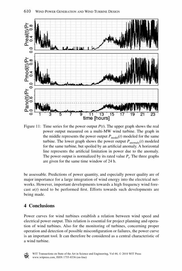
A simple, artifi cial case was created in Fig. 11 . In this fi gure, one can see the real power output P ( t ) of a wind turbine, then the same quantity modeled in good running condition, and fi nally modeled with an artifi cial anomaly (that limits the power extraction to roughly 45% of the rated power P r ). A comparison of the fi rst and second graph shows that through a simple model, it is possible to estimate the power output P ( t ) of a wind turbine knowing only D (1)( P ; u ) and D (2)( P ; u ). This model can be applied to any wind situation u ( t ), as an effective way to study the behavior of a wind turbine in different wind conditions.

This model shows great potential in the continuing evolution of current methods, principally in the prediction of power production. When coupled with a meteoro-logical wind forecast, the model could be used to generate the power output of a wind turbine (whose power performance has been characterized). In addition to providing quantitative power production estimates, power quality, i.e. fl uctuations in power, stability, and regularity of the high frequency power output P ( t ) too will



be assessable. Predictions of power quantity, and especially power quality are of major importance for a large integration of wind energy into the electrical net-works. However, important developments towards a high frequency wind fore-cast u ( t ) need to be performed fi rst. Efforts towards such developments are being made.

4 Conclusions

Power curves for wind turbines establish a relation between wind speed and electrical power output. This relation is essential for project planning and opera-tion of wind turbines. Also for the monitoring of turbines, concerning proper operation and detection of possible misconfi guration or failures, the power curve is an important tool. It can therefore be considered as a central characteristic of a wind turbine.

Figure 11 : Time series for the power output P ( t ). The upper graph shows the real power output measured on a multi-MW wind turbine. The graph in the middle represents the power output P model ( t ) modeled for the same turbine. The lower graph shows the power output P anomaly ( t ) modeled for the same turbine, but spoiled by an artifi cial anomaly. A horizontal line represents the artifi cial limitation in power due to the anomaly. The power output is normalized by its rated value P r . The three graphs are given for the same time window of 24 h.



The current industry standard IEC 61400-12-1 [ 3 ] defi nes, among others, a uniform procedure for the measurement of power curves. This defi nition relies on temporal averaging of wind speed and power output. Due to the turbulent nature of the wind and the non-linear dependency of power on wind speed, this power curve combines the characteristic of the turbine together with the statistical features of the wind at the special site under investigation. This combination makes the esti-mation of the annual energy yield at a certain site especially easy. On the other hand, systematic averaging errors are introduced through the mentioned non-linearity, and the power characteristic of the turbine cannot be separated from the site effects. These weaknesses are well known, and several corrections have been proposed, e.g. [ 19 ].

As an alternative, recently a different approach has been proposed to obtain the power characteristic of wind turbines [ 16 , 17 ], the Langevin power curve, which relies on high frequency measurement data (approximately 1 Hz). Inspired from dynamical systems theory, the power conversion process is regarded as a relax-ation process, driven by the turbulently fl uctuating wind speed. The power charac-teristic can then be obtained for every wind speed as the stable fi xed points of this process. Averaging errors and infl uence of turbulence are thus avoided. Possible multiple stable states are also captured, allowing deeper insight in the dynamics of the power conversion. These features make the dynamical power characteristic especially interesting as a monitoring tool for wind turbines.

As a work in progress, the simulation of high frequency power output signals based on eqn ( 8 ) is currently developed. One application of this procedure will be the prediction of energy yields for specifi c wind turbines under specifi c wind conditions.

References

[ 1] Gottschall, J. & Peinke, J., Stochastic modelling of a wind turbine’s power output with special respect to turbulent dynamics. J. Phys: Conf Ser , 75 , pp. 012045, 2007.

[2] Burton, T., Sharpe, D., Jenkins, N. & Bossanyi, E., Wind Energy Handbook , Wiley: New York, 2001.

[3] IEC. Wind turbine generator systems, Part 12: Wind turbine power performance testing, International Standard 61400-12-1, International Electrotechnical Commission, 2005.

[4] Böttcher, F., Barth, S. & Peinke, J., Small and large fl uctuations in atmospheric wind speeds. Stochastic Environmental Research and Risk Assessment , 2 1, pp. 299–308, 2007.

[5] Betz, A., Die Windmühlen im Lichte neuerer Forschung. Die Naturwissen-schaften , 15 , pp. 46, 1927.

[6] Rauh, A. & Seelert, W., The Betz optimum effi ciency for windmills. Applied Energy , 17 , pp. 15–23, 1984.

[7] Rauh, A., On the relevance of basic hydrodynamics to wind energy technology. Nonlinear Phenomena in Complex Systems , 11 (2), pp. 158–163, 2008.



[8] Bianchi, F., De Battista, H. & Mantz, R., Wind Turbine Control Systems , 2nd ed., Springer: Berlin, 2006.

[9] Hanse, A., Jauch, C., Soerense, P., Iov, F. & Blaabjerg, F., Dynamic wind turbine models in power system simulation tool DIgSILENT, Risø Report Risø-R-1400(EN), Risø National Laboratory, 2003.

[ 10] Böttcher, F., Peinke, J., Kleinhans, D. & Friedrich, R., Handling systems driven by different noise sources – Implications for power estimations. Wind Energy , Springer: Berlin, pp. 179–182, 2007.

[ 11] Wächter, M., Gottschall, J., Rettenmeier, A. & Peinke, J., Dynamical power curve estimation using different anemometer types. Proc. of DEWEK , Bremen, Germany, 2008.

[ 12] Rettenmeier, A., Kühn, M., Wächter, M., Rahm, S., Mellinghoff, H., Siegmeier, B. & Reeder, L., Development of LiDAR measurements for the German offshore test site. IOP Conference Series: Earth and Environmental Science , 1 , pp. 012063 (6 pages), 2008.

[ 13] Rosen, A. & Sheinman, Y., The average power output of a wind turbine in turbulent wind. Journal of Wind Engineering and Industrial Aerodynamics , 51 , pp. 287–302, 1994.

[ 14] Rauh, A. & Peinke, J., A phenomenological model for the dynamic response of wind turbines to turbulent wind. Journal of Wind Engineering and Industrial Aerodynamics , 92 (2), pp. 159–183, 2004.

[15] Risken, H., The Fokker-Planck Equation , Springer: Berlin, 1984. [ 16] Gottschall, J. & Peinke, J., How to improve the estimation of power curves for

wind turbines. Environmental Research Letters , 3 (1), pp. 015005 (7 pages), 2008.

[17] Anahua, E., Barth, S. & Peinke, J., Markovian power curves for wind turbines. Wind Energy , 11 (3), pp. 219–232, 2008.

[18] Gottschall, J. & Peinke, J., Power curves for wind turbines – a dynamical approach. Proc. of EWEC 2008 , Brussels, Belgium, 2008.

[ 19] Albers, A., Jakobi, T., Rohden, R. & Stoltenjohannes, J., Infl uence of meteoro logical variables on measured wind turbine power curves. Proc. of EWEC 2007 , Milan, Italy, 2007.


CHAPTER 18 Power curves for wind turbines...The more complex shape of a real wind turbine cer-tainly...

Documents

Transcript of CHAPTER 18 Power curves for wind turbines...The more complex shape of a real wind turbine cer-tainly...