Chapter 16 Local Operations - RIT
64
Chapter 16 Local Operations g[x, y]= O{f [x ± ∆x, y ± ∆y]} In many common image processing operations, the output pixel is a weighted com- bination of the gray values of pixels in the neighborhood of the input pixel, hence the term local neighborhood operations. The size of the neighborhood and the pixel weights determine the action of the operator. This concept has already been intro- duced when we considered image prefiltering during the discussion of realistic image sampling. It will now be formalized and will serve as the basis of the discussion of image transformations. Schematic of a local operation applied to the input image f [x, y] to create the output image g [x, y]. The local operation weights the gray values in the neighborhood of the input pixel. 371
Transcript of Chapter 16 Local Operations - RIT

Chapter 16
Local Operations
g[x, y] = O{f [x±∆x, y ±∆y]}In many common image processing operations, the output pixel is a weighted com-bination of the gray values of pixels in the neighborhood of the input pixel, hencethe term local neighborhood operations. The size of the neighborhood and the pixelweights determine the action of the operator. This concept has already been intro-duced when we considered image prefiltering during the discussion of realistic imagesampling. It will now be formalized and will serve as the basis of the discussion ofimage transformations.
Schematic of a local operation applied to the input image f [x, y] to create the outputimage g [x, y]. The local operation weights the gray values in the neighborhood of the
input pixel.
371
372 CHAPTER 16 LOCAL OPERATIONS
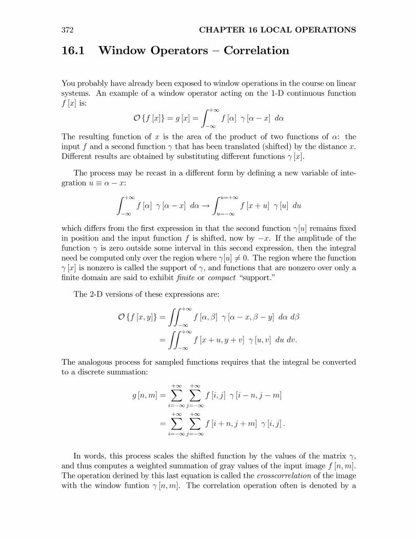
16.1 Window Operators — Correlation
You probably have already been exposed to window operations in the course on linearsystems. An example of a window operator acting on the 1-D continuous functionf [x] is:
O{f [x]} = g [x] =
Z +∞
−∞f [α] γ [α− x] dα
The resulting function of x is the area of the product of two functions of α: theinput f and a second function γ that has been translated (shifted) by the distance x.Different results are obtained by substituting different functions γ [x].
The process may be recast in a different form by defining a new variable of inte-gration u ≡ α− x:Z +∞
−∞f [α] γ [α− x] dα→
Z u=+∞
u=−∞f [x+ u] γ [u] du
which differs from the first expression in that the second function γ[u] remains fixedin position and the input function f is shifted, now by −x. If the amplitude of thefunction γ is zero outside some interval in this second expression, then the integralneed be computed only over the region where γ[u] 6= 0. The region where the functionγ [x] is nonzero is called the support of γ, and functions that are nonzero over only afinite domain are said to exhibit finite or compact “support.”
The 2-D versions of these expressions are:
O{f [x, y]} =ZZ +∞
−∞f [α, β] γ [α− x, β − y] dα dβ
=
ZZ +∞
−∞f [x+ u, y + v] γ [u, v] du dv.
The analogous process for sampled functions requires that the integral be convertedto a discrete summation:
g [n,m] =+∞X
i=−∞
+∞Xj=−∞
f [i, j] γ [i− n, j −m]
=+∞X
i=−∞
+∞Xj=−∞
f [i+ n, j +m] γ [i, j] .
In words, this process scales the shifted function by the values of the matrix γ,and thus computes a weighted summation of gray values of the input image f [n,m].The operation derined by this last equation is called the crosscorrelation of the imagewith the window funtion γ [n,m]. The correlation operation often is denoted by a

16.1 WINDOW OPERATORS — CORRELATION 373
five-pointed star (“pentagram”), e.g.,
g [n,m] = f [n,m]F [n,m]
=+∞X
i=−∞
+∞Xj=−∞
f [i, j] γ [i− n, j −m]
The output image g at pixel indexed by [n,m] is computed by centering the windowγ [n,m] on that pixel of the input image f [n,m], multiplying the window and inputimage pixel by pixel, and summing the products. This operation produces an outputextremum at shifts [n,m] where the gray-level pattern of the input matches that ofthe window.In the common case where the sampled function γ is zero outside a domain with
compact support of size 3× 3 samples, the function may be written in the form of a3× 3 matrix or window function:
γ [n,m] =
γ−1,1 γ0,1 γ1,1
γ−1,0 γ0,0 γ1,0
γ−1,−1 γ0,−1 γ1,−1
,
16.1.1 Examples of 3× 3 Crosscorrelation OperatorsConsider the action of these 3× 3 window functions:
γ1 [n,m] =
0 0 0
0 +1 0
0 0 0
γ2 [n,m] =
0 0 0
0 +2 0
0 0 0
γ1 [n,m] =
0 0 0
0 0 +1
0 0 0
• γ1— the only pixel that influences the output g [n,m] is the identical pixel in theinput f [n,m] — this is the identity operator.
• γ2— the output pixel has twice the gray value of the input pixel — this is auniform contrast stretching operator.

374 CHAPTER 16 LOCAL OPERATIONS
• γ3— the output pixel is identical to its right-hand neighbor in the input image —this operator translates the image one pixel to the left.
Once the general crosscorrelation algorithm is programmed, many useful opera-tions on the image f [n,m] can be performed simply by specifying different values forthe window coefficients.
16.2 Convolution
Amathematically equivalent but generally more convenient neighborhood operation isthe convolution, which has some very nice mathematical properties. The convolutionof two 1-D continuous functions, the input f [x] and the impulse response (or kernel,or point spread function, or system function) h [x] is:
g [x] = f [x] ∗ h [x] ≡Z ∞
−∞dα f [α] h [x− α] .
where α is a dummy variable of integration. As for the crosscorrelation, the functionh [x] defines the action of the system on the input f [x]. By changing the integrationvariable to u ≡ x− α, an equivalent expression for the convolution is found:
g [x] =
Z ∞
−∞f [α] h [x− α] dα
=
Z u=+∞
u=+∞f [x− u] h [u] (−du)
=
Z ∞
−∞f [x− u] h [u] du
=
Z ∞
−∞h [α] f [x− α] dα
where the dummy variable was renamed from u to α in the last step. Note thatthe roles of f [x] and h [x] have been exchanged between the first and last expres-sions, which means that the input function f [x] and system function h [x] can beinterchanged.The convolution of a continuous 2-D function f [x, y] with a system function h[x, y]
is denoted by an asterisk “∗” and defined as:
g [x, y] = f [x, y] ∗ h [x, y]
≡ZZ ∞
−∞f [α, β] h [x− α, y − β] dα dβ
=
ZZ ∞
−∞f [x− α, y − β] h [α, β] dα dβ
Note the difference between the first forms for the convolution and the crosscorrela-

16.2 CONVOLUTION 375
tion:
f [x, y]F [x, y] =ZZ ∞
−∞f [α, β] γ [α− x, β − y] dα dβ
f [x, y] ∗ h [x, y] ≡ZZ ∞
−∞f [α, β] h [x− α, y − β] dα dβ
and between the second forms:
f [x, y]F [x, y] ≡ZZ ∞
−∞f [x+ u, y + v] γ [u, v] du dv
f [x, y] ∗ h [x, y] ≡ZZ ∞
−∞f [x− α, y − β] h [α, β] dα dβ
The changes of the order of the variables in the first pair says that the function γis just shifted before multiplying by f in the crosscorrelation, while the function his flipped about its center (or equivalently rotated about the center by 180◦) beforeshifting. In the second pair, the difference in sign of the integration variables saysthat the input function f is shifted in different directions before multiplying by thesystem function γ for crosscorrelation and h for convolution. In convolution, it iscommon to speak of filtering the input f with the kernel h. For discrete functions,the convolution integral becomes a summation:
g [n,m] = f [n,m] ∗ h [n,m]
≡∞X
i=−∞
∞Xj=−∞
f [i, j] h [n− i,m− j] .
Again, note the difference in algebraic sign of the action of the kernel h [n,m] inconvolution and the window γij in correlation:
f [n,m]F [n,m] =∞X
i=−∞
∞Xj=−∞
f [i, j] γ [i− n, j −m]
f [n,m] ∗ h [n,m] =∞X
i=−∞
∞Xj=−∞
f [i, j] h [n− i,m− j] .
This form of the convolution has the very useful property that convolution of an inputin the form of an impulse function δd [n,m] with h [n,m] yields h [n,m], hence thename for h as the impulse response:
δd [n,m] ∗ h [n,m] = h [n,m]
376 CHAPTER 16 LOCAL OPERATIONS
where the discrete Dirac delta function δd [n,m] is defined:
δd [n,m] ≡
⎧⎨⎩ 1 if n = m = 0
0 otherwise
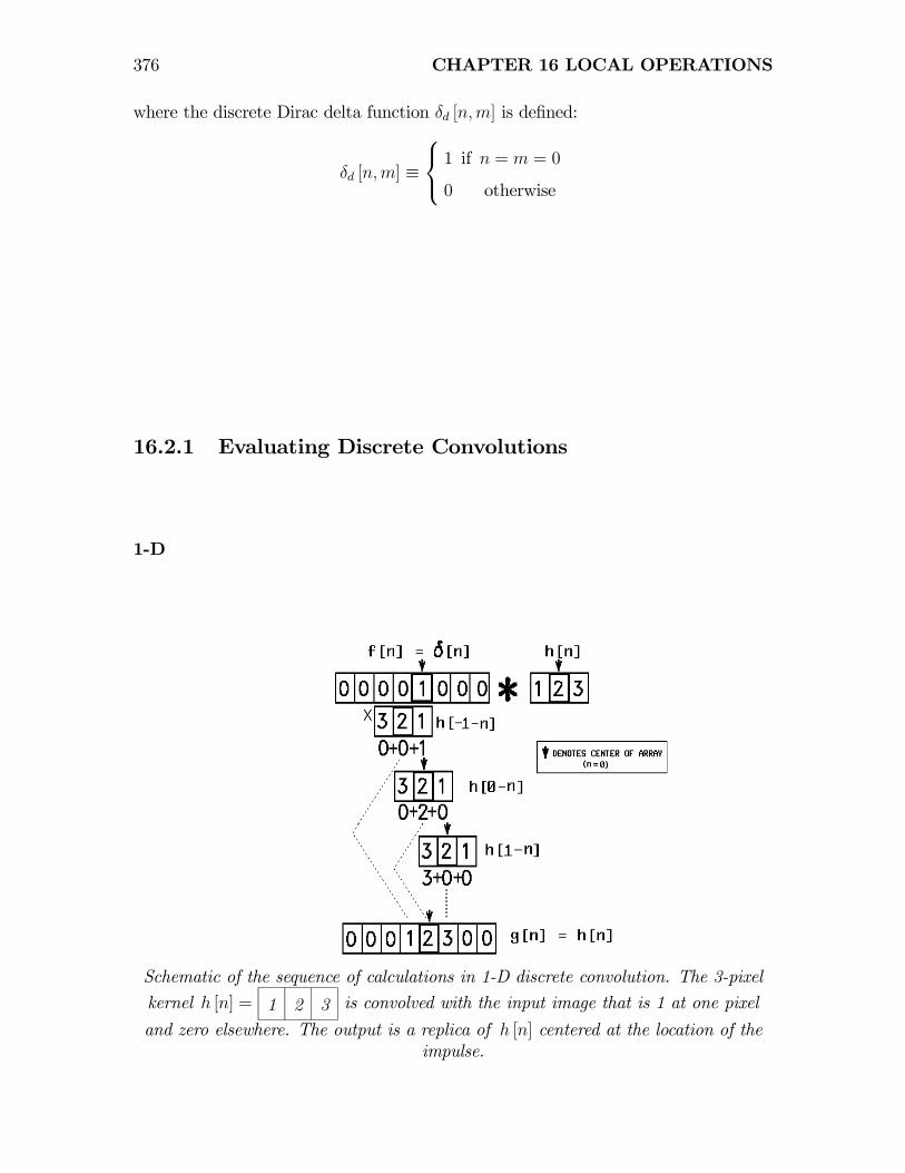
16.2.1 Evaluating Discrete Convolutions
1-D
Schematic of the sequence of calculations in 1-D discrete convolution. The 3-pixel
kernel h [n] = 1 2 3 is convolved with the input image that is 1 at one pixel
and zero elsewhere. The output is a replica of h [n] centered at the location of theimpulse.

16.2 CONVOLUTION 377
2-D
Schematic of 2-D discrete convolution with the 2-D kernel h [n,m].
δ [i− n, j −m] ∗ h[n,m] = h [n,m]
Examples of 2-D Convolution Kernels
0 0 0
0 +1 0
0 0 0
=⇒ identity
0 0 0
0 0 +1
0 0 0
=⇒ shifts image one pixel to right
Discrete convolution is linear because it is defined by a weighted sum of pixel grayvalues:
f [n,m] ∗ (h1 [n,m] + h2 [n,m]) ≡+∞X
i=−∞
+∞Xj=−∞
f [i, j] · (h1 [n− i,m− j] + h2 [n− i,m− j])
=+∞X
i=−∞
+∞Xj=−∞
(f [i, j] · h1 [n− i,m− j] + f [i, j] · h2 [n− i,m− j])
=+∞X
i=−∞
+∞Xj=−∞
f [i, j] · h1 [n− i,m− j] ++∞X
i=−∞
+∞Xj=−∞
f [i, j] · h2 [n− i,m− j]
378 CHAPTER 16 LOCAL OPERATIONS
f [n,m] ∗ (h1 [n,m] + h2 [n,m]) = f [n,m] ∗ h1 [n,m] + f [n,m] ∗ h2 [n,m]
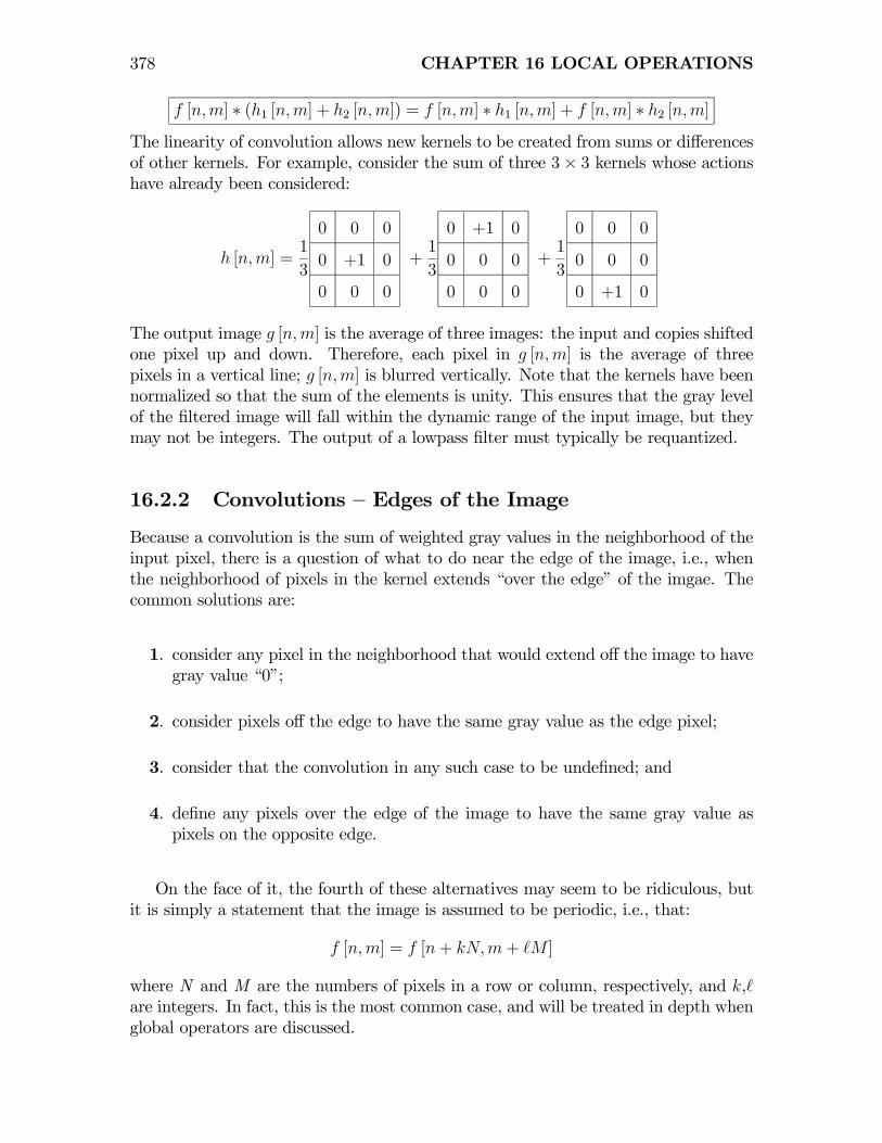
The linearity of convolution allows new kernels to be created from sums or differencesof other kernels. For example, consider the sum of three 3× 3 kernels whose actionshave already been considered:
h [n,m] =1
3
0 0 0
0 +1 0
0 0 0
+1
3
0 +1 0
0 0 0
0 0 0
+1
3
0 0 0
0 0 0
0 +1 0
The output image g [n,m] is the average of three images: the input and copies shiftedone pixel up and down. Therefore, each pixel in g [n,m] is the average of threepixels in a vertical line; g [n,m] is blurred vertically. Note that the kernels have beennormalized so that the sum of the elements is unity. This ensures that the gray levelof the filtered image will fall within the dynamic range of the input image, but theymay not be integers. The output of a lowpass filter must typically be requantized.
16.2.2 Convolutions — Edges of the Image
Because a convolution is the sum of weighted gray values in the neighborhood of theinput pixel, there is a question of what to do near the edge of the image, i.e., whenthe neighborhood of pixels in the kernel extends “over the edge” of the imgae. Thecommon solutions are:
1. consider any pixel in the neighborhood that would extend off the image to havegray value “0”;
2. consider pixels off the edge to have the same gray value as the edge pixel;
3. consider that the convolution in any such case to be undefined; and
4. define any pixels over the edge of the image to have the same gray value aspixels on the opposite edge.
On the face of it, the fourth of these alternatives may seem to be ridiculous, butit is simply a statement that the image is assumed to be periodic, i.e., that:
f [n,m] = f [n+ kN,m+ M ]
where N and M are the numbers of pixels in a row or column, respectively, and k,are integers. In fact, this is the most common case, and will be treated in depth whenglobal operators are discussed.

16.2 CONVOLUTION 379
Possible strategies for dealing with the edge of the image in 2-D convolution: (a) theinput image is padded with zeros; (b) the input image is padded with the same grayvalues “on the edge;” (c) values “off the edge” are ignored; (d) pixels off the edge are
assigned the values on the opposite edge, this assumes that the input image isperiodic.
The 3 × 3 image f [n,m] is outlined by the bold-face box and the assumed grayvalues of pixels off the edge of the image are shown in light face for four cases; thepresence of an “x” in a convolutio kernel indicates that the output gray value isundefined.
16.2.3 Convolutions — Computational Intensity
Evaluating convolutions with large kernels in a serial processor used to be very slow.For example, convolution of a 5122-pixel image with an M × M kernel requires:2·5122 ·M2 operations (multiplications and additions) for a total of 4.7·106 operationswith a 3× 3 kernel and 25.7 · 106 operations with a 7× 7 (these operations generallyare performed on floating-point data). The increase in computations as M2 ensuresthat convolution of large images with large kernels is not very practical by serialbrute-force means. In the discussion of global operations to follow, we will introducean alternative method for computing convolutions via the Fourier transform thatrequires many fewer operations for large images.
16.2.4 Smoothing Kernels — Lowpass Filtering
If all elements of a convolution kernel have the same algebraic sign, then the operatorO sums weighted gray values of input pixels in the neighborhood; if the sum of theelements is one, then the process computes a weighted average of the gray values.Averaging reduces the variability of the gray values of the input image; it “smooths”the function:

380 CHAPTER 16 LOCAL OPERATIONS
Local averaging decreases the “variability” (variance) of pixel gray values
For a uniform averaging kernel of a fixed size, functions that oscillate over a period justlonger than the kernel (e.g., short-period, high-frequency sinusoids) will be averagedmore than slowly varying terms. In other words, local averaging attenuates the highsinusoidal frequencies while passing the low frequencies relatively undisturbed — localaveraging operators are lowpass filters. If the kernel size doubles, input sinusoidswith twice the period (half the spatial frequency) will be equivalently affected. Thisaction was discussed in the section on realistic sampling; a finite detector averagesthe signal over its width and reduces modulation of the output signal to a greaterdegree at higher frequencies.
Local averaging operators are lowpass filters
Obviously, averaging kernels reduce the visibility of additive noise by spreading thedifference in gray value of noise pixel from the background over its neighbors. Byanalogy with temporal averaging, spatial averaging of noise increases SNR by thesquare-root of the number of pixels averaged if the noise is random and the averagingweights are identical.
The action of an averager can be directional:
h1 [n,m] =1
3
0 +1 0
0 +1 0
0 +1 0
averages vertically
h2 [n,m] =1
3
0 0 0
+1 +1 +1
0 0 0
blurs horizontally
h3 [n,m] =1
3
+1 0 0
0 +1 0
0 0 +1
blurs diagonally
The “rotation” or “reversal” of the convolution kernel means that the action ofh3 [n,m] blurs diagonally along the direction at 90◦ that in the kernel.

16.2 CONVOLUTION 381
The elements of an averaging kernel need not be identical, e.g.,
h [n,m] =1
3
+14+14+14
+14+1 +1
4
+14+14+14
averages over the entire window but the output is primarily influenced by the centerpixel; the output blurred less than in the case when all elements are identical.
Other 2-D discrete averaging kernels may be constructed by “orthogonal multipli-cation,” e.g., we can construct the common 3 × 3 uniform averager via the productof two orthogonal 1-D uniform averagers:
+13+13+13·+13
+13
+13
=
13· 13
13· 13
13· 13
13· 13
13· 13
13· 13
13· 13
13· 13
13· 13
=
+19+19+19
+19+19+19
+19+19+19
The associated transfer function is the orthogonal product of the individual 1-D trans-fer functions. Note that the 1-D kernels can be different, such as a 3-pixel uniformaverager along the n-direction and a 2-pixel uniform averager along m:
+13+13+13·+14
+12
+14
=
13· 14
13· 14
13· 14
13· 12
13· 12
13· 12
13· 14
13· 14
13· 14
=
+ 112
+ 112
+ 112
+16
+16
+16
+ 112
+ 112
+ 112
Lowpass-Filtered Images
Examples of lowpass filtering: (a) f [n,m]; (b) after uniform averaging over a 3× 3neighborhood; (c) after uniform averaging over a 5× 5 neighborhood. Note that the“fine structure” (such as it is) becomes less visible as the neighborhood size increases.
382 CHAPTER 16 LOCAL OPERATIONS
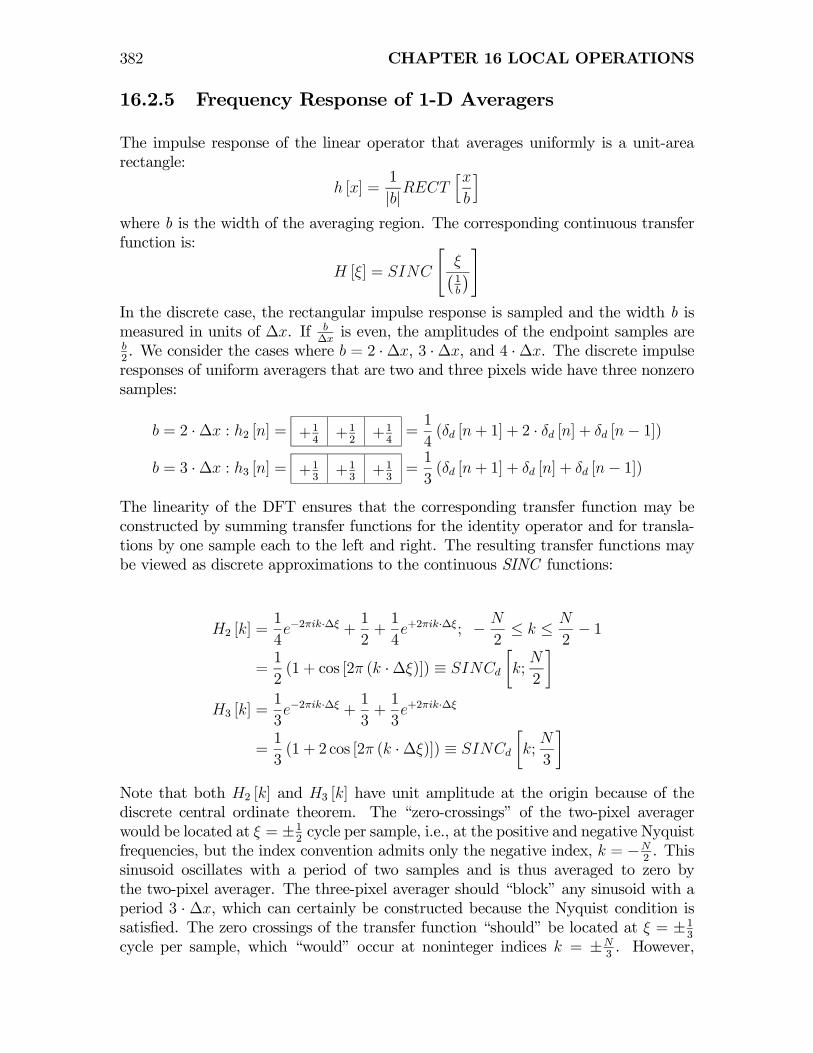
16.2.5 Frequency Response of 1-D Averagers
The impulse response of the linear operator that averages uniformly is a unit-arearectangle:
h [x] =1
|b|RECThxb
iwhere b is the width of the averaging region. The corresponding continuous transferfunction is:
H [ξ] = SINC
"ξ¡1b
¢#In the discrete case, the rectangular impulse response is sampled and the width b ismeasured in units of ∆x. If b
∆xis even, the amplitudes of the endpoint samples are
b2. We consider the cases where b = 2 ·∆x, 3 ·∆x, and 4 ·∆x. The discrete impulseresponses of uniform averagers that are two and three pixels wide have three nonzerosamples:
b = 2 ·∆x : h2 [n] = +14+12+14=1
4(δd [n+ 1] + 2 · δd [n] + δd [n− 1])
b = 3 ·∆x : h3 [n] = +13+13+13=1
3(δd [n+ 1] + δd [n] + δd [n− 1])
The linearity of the DFT ensures that the corresponding transfer function may beconstructed by summing transfer functions for the identity operator and for transla-tions by one sample each to the left and right. The resulting transfer functions maybe viewed as discrete approximations to the continuous SINC functions:
H2 [k] =1
4e−2πik·∆ξ +
1
2+1
4e+2πik·∆ξ; − N
2≤ k ≤ N
2− 1
=1
2(1 + cos [2π (k ·∆ξ)]) ≡ SINCd
∙k;
N
2
¸H3 [k] =
1
3e−2πik·∆ξ +
1
3+1
3e+2πik·∆ξ
=1
3(1 + 2 cos [2π (k ·∆ξ)]) ≡ SINCd
∙k;
N
3
¸Note that both H2 [k] and H3 [k] have unit amplitude at the origin because of thediscrete central ordinate theorem. The “zero-crossings” of the two-pixel averagerwould be located at ξ = ±1
2cycle per sample, i.e., at the positive and negative Nyquist
frequencies, but the index convention admits only the negative index, k = −N2. This
sinusoid oscillates with a period of two samples and is thus averaged to zero bythe two-pixel averager. The three-pixel averager should “block” any sinusoid with aperiod 3 · ∆x, which can certainly be constructed because the Nyquist condition issatisfied. The zero crossings of the transfer function “should” be located at ξ = ±1
3
cycle per sample, which “would” occur at noninteger indices k = ±N3. However,
16.2 CONVOLUTION 383
because ±N3is not an integer when N is even, the zero crossings of the spectrum
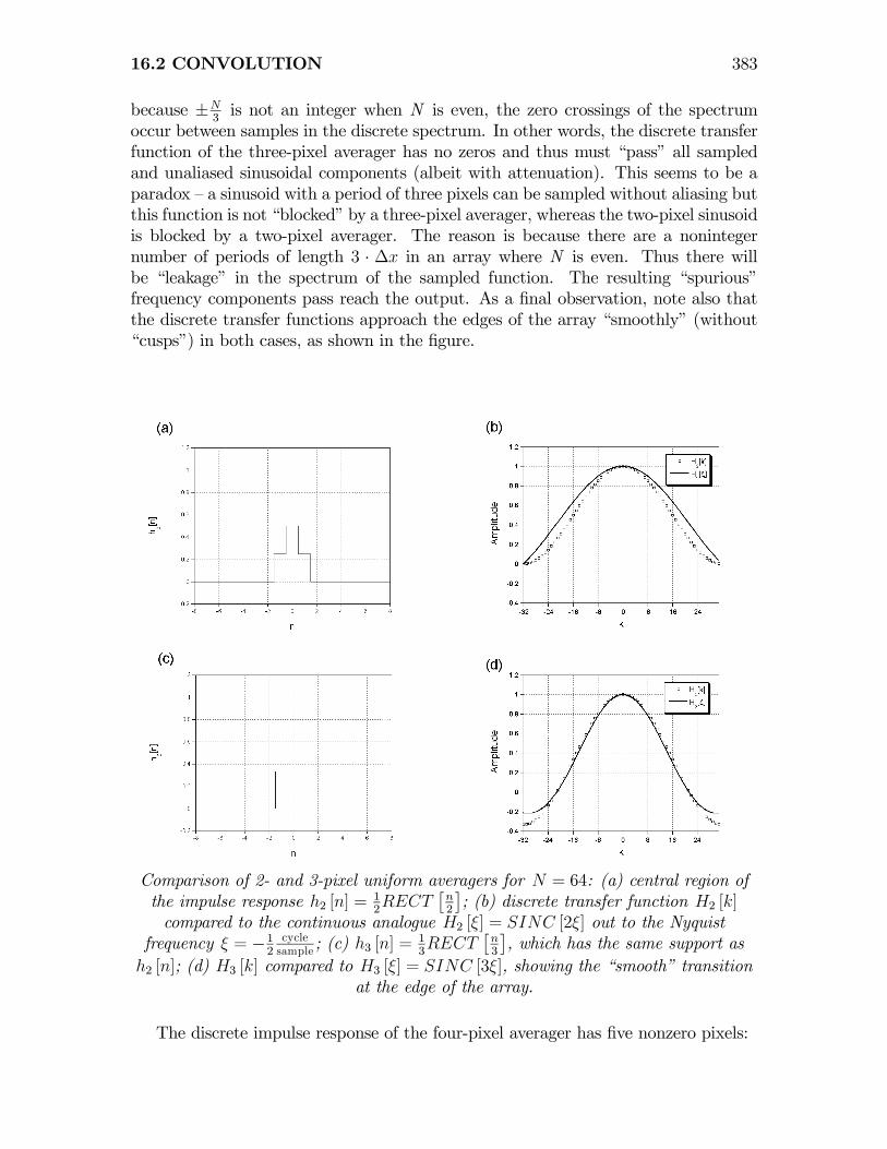
occur between samples in the discrete spectrum. In other words, the discrete transferfunction of the three-pixel averager has no zeros and thus must “pass” all sampledand unaliased sinusoidal components (albeit with attenuation). This seems to be aparadox — a sinusoid with a period of three pixels can be sampled without aliasing butthis function is not “blocked” by a three-pixel averager, whereas the two-pixel sinusoidis blocked by a two-pixel averager. The reason is because there are a nonintegernumber of periods of length 3 · ∆x in an array where N is even. Thus there willbe “leakage” in the spectrum of the sampled function. The resulting “spurious”frequency components pass reach the output. As a final observation, note also thatthe discrete transfer functions approach the edges of the array “smoothly” (without“cusps”) in both cases, as shown in the figure.
Comparison of 2- and 3-pixel uniform averagers for N = 64: (a) central region ofthe impulse response h2 [n] =
12RECT
£n2
¤; (b) discrete transfer function H2 [k]
compared to the continuous analogue H2 [ξ] = SINC [2ξ] out to the Nyquistfrequency ξ = −1
2cyclesample ; (c) h3 [n] =
13RECT
£n3
¤, which has the same support as
h2 [n]; (d) H3 [k] compared to H3 [ξ] = SINC [3ξ], showing the “smooth” transitionat the edge of the array.
The discrete impulse response of the four-pixel averager has five nonzero pixels:

384 CHAPTER 16 LOCAL OPERATIONS
b = 4 ·∆x : h4 [n] = +18+14+14+14+18
The linearity of the DFT ensures that the corresponding transfer function may beconstructed by summing the transfer function of the three-pixel averager scaled by 3
4
with the transfer functions for translation by two samples each to the left and right:
H4 [k] =1
4
µ1
2e−2πik·2∆ξ + e−2πik·∆ξ + 1 + e+2πik·∆ξ +
1
2e+2πik·2∆ξ
¶=1
4(1 + 2 cos [2π (k ·∆ξ)] + cos [2π (k · 2∆ξ)])
which also may be thought of as a discrete approximation of a SINC function:SINCd
£k; N
4
¤. This discrete transfer function has zeros located at ξ = ±1
4cycle
per sample, which correspond to k = ±N4. Therefore the four-pixel averager “blocks”
any sampled sinusoid with period 4 ·∆x from reaching the output. Again the trans-fer function has “smooth” transitions of amplitude at the edges of the array, thuspreventing “cusps” in the periodic spectrum, as shown in the figure.
Four-pixel averager for N = 64: (a) central region of impulse responseh4 [n] =
14RECT
£n4
¤; (b) Discrete transfer function H4 [k] compared to the
continuous transfer function SINC [4ξ], showing the smooth decay of the discretecase at the edges of the array.
16.2 CONVOLUTION 385
The general expression for the discrete SINC function in the frequency domainsuggested by these results for −N
2≤ k ≤ N
2− 1 is:
SINCd
∙k;
N
w
¸=⎧⎪⎪⎪⎪⎪⎪⎨⎪⎪⎪⎪⎪⎪⎩
1w
⎛⎝1 + 2w−12X=1
cos [2π (k · ·∆ξ)]
⎞⎠ if w is odd
1w
⎛⎝1 + cos £2π ¡k · w2·∆ξ
¢¤+ 2
w2−1X=1
cos [2π (k · ·∆ξ)]
⎞⎠ if w is even
16.2.6 2-D Averagers
Effect of Lowpass Filtering on the Histogram
Because an averaging kernel reduces pixel-to-pixel variations in gray level (and hencethe variance of additive random noise in the image), we would expect that clustersof pixels in the histogram of an averaged image to be taller and thinner than in theoriginal image. It should be easier to segment objects based on average gray level fromthe histogram of an averaged image. To illustrate, we reconsider the example of thehouse-tree image. The image in blue light and its histogram before and after averagingwith a 3× 3 kernel are shown below: Note that there are four fairly distinct clustersin the histogram of the averaged image, corresponding to the house, grass+tree, sky,and clouds+door (from dark to bright). The small clusters at the ends are moredifficult to distinguish on the original histogram.

386 CHAPTER 16 LOCAL OPERATIONS
Effect of blurring on the histogram: the 64× 64 color image, the histograms of the 3bands, and the 3 2-D histograms are shown at top; the same images and histogramsafter blurring with a 3× 3 kernel are at the bottom, showing the concentration of
histogram clusters resulting from image blur.
Note that the noise visible in uniform areas of the images (e.g., the sky in theblue image) has been noticeably reduced by the averaging, and thus the widths of thehistogram clusters have decreased. The downside of this process is that pixels on theboundaries of objects now exhibit blends of the colors of both bounding objects, andthus will not be as easy to segment.
16.2.7 Differencing Kernels — Highpass Filters
A kernel with both positive and negative terms computes differences of neighboringpixels. From the previous discussion, it is probably apparent that the converse of the

16.2 CONVOLUTION 387
statement about local averaging also is true.
Local Differencing increases the variance of pixel gray values
The difference of adjacent pixels with identical gray levels will cancel out, whiledifferences between adjacent pixels will be amplified. Since high-frequency sinusoidsvary over shorter distances, differencing operators will enhance them and attenuateslowly varying (i.e., lower-frequency) terms.
Differencing operators are highpass filters
because a differencing operator twill “block” low-frequency sinusoids and “pass” thosewith high frequencies.Subtraction of adjacent pixels can result in negative gray values; this is the spatial
analogy of temporal differencing for change detection. The gray values of the outputimage must be biased “up” for display by adding some constant gray level to all imagepixels, e.g., if gmin < 0, then the negative gray values may be displayed by adding thelevel |gmin| to all pixel gray values.The discrete analogue of differentiation may be derived from the definition of the
continuous derivative:df
dx≡ lim
τ→0
µf [x+ τ ]− f [x]
τ
¶In the discrete case, the smallest nonzero value of τ is the sampling interval ∆x, andthus the discrete derivative is:
1
∆x(f [(n+ 1) ·∆x]− f [n ·∆x]) =
1
∆xf [n ·∆x] ∗ (δ [n+ 1]− δ [n])
In words, the discrete derivative is the scaled difference of the value at the sampleindexed by n+ 1 and by n. By setting ∆x = 1 sample, the leading scale factor maybe ignored. The 1-D derivative operator may be implemented by discrete convolutionwith a 1-D kernel that has two nonzero elements; we will write it with three elementsto clearly denote the sample indexed by n = 0.
f [n] ∗ (δ [n+ 1]− δ [n]) = f [n] ∗ +1 −1 0 ≡ f [n] ∗ ∂ [n]
where ∂ [n] ≡ +1 −1 0 is the discrete impulse response of differentiation, which
is perhaps better called a differencing operator. Note that the impulse response maybe decomposed into its even and odd parts.
∂even [n] = +12−1 +1
2
=
µ+1
2
¶+1 +1 +1 −
µ+3
2
¶0 +1 0
∂odd [n] = +120 −1
2=
µ+1
2
¶+1 0 −1
388 CHAPTER 16 LOCAL OPERATIONS
The even part is a weighted difference of the identity operator and the three-pixelaverager, while the odd part computes differences of pixels separated by two sampleintervals.
The corresponding 2-D derivative kernel in the x-direction is:
h [n,m] =
0 0 0
+1 −1 0
0 0 0
=
0 0 0
+1 0 0
0 0 0
+
0 0 0
0 −1 0
0 0 0
=
0 0 0
+1 0 0
0 0 0
−0 0 0
0 +1 0
0 0 0
≡ ∂x
The resulting image is equivalent to the difference between an image translated onepixel to the left and an unshifted image, i.e.,
∂
∂xf [x, y] = lim
∆x→0
f [x+∆x, y]− f [x, y]
∆x
=⇒ ∂
∂xf [x, y] ≡ f [(n+ 1) ·∆x,m ·∆y]− f [n ·∆x,m ·∆y]
=⇒ ∂x ∗ f [n,m] = f [n+ 1,m]− f [n,m]
because the minimum nonzero value of the translation ∆x = 1 sample. The corre-sponding discrete partial derivative in the y-direction is:
∂y ∗ f [n,m] ≡ f [n,m+ 1]− f [n,m]
The partial derivative in the y-direction is the difference of a replica translated“up” and the original:
∂y =
0 +1 0
0 −1 0
0 0 0
This definition of the derivative effectively “locates” the edge of an object at the pixelimmediately to the right or above the “crack” between pixels that is the actual edge.
16.2 CONVOLUTION 389
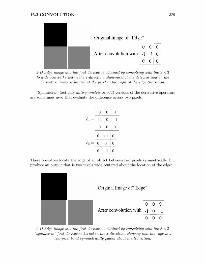
2-D Edge image and the first derivative obtained by convolving with the 3× 3first-derivative kernel in the x-direction, showing that the detected edge in thederivative image is located at the pixel to the right of the edge transition.
“Symmetric” (actually antisymmetric or odd) versions of the derivative operatorsare sometimes used that evaluate the difference across two pixels:
∂x =
0 0 0
+1 0 −1
0 0 0
∂y =
0 +1 0
0 0 0
0 −1 0
These operators locate the edge of an object between two pixels symmetrically, butproduce an output that is two pixels wide centered about the location of the edge:
2-D Edge image and the first derivative obtained by convolving with the 3× 3“symmetric” first-derivative kernel in the x-direction, showing that the edge is a
two-pixel band symmetrically placed about the transition.

390 CHAPTER 16 LOCAL OPERATIONS
Higher-Order Derivatives
The kernels for higher-order derivatives are easily computed because convolution isassociative. The convolution kernel for the 1-D second derivative is obtained byautoconvolving the kernel for the 1-D first derivative:
∂2
∂x2f [x, y] =
∂
∂x
µ∂
∂xf [x, y]
¶=
∂
∂x
µlim∆x→0
f [x+∆x, y]− f [x, y]
∆x
¶= lim
∆x→0
µlim∆x→0
µf [x+ 2 ·∆x, y]− f [x+∆x, y]
∆x
¶− lim
∆x→0
µf [x+∆x, y]− f [x, y]
∆x
¶¶= lim
∆x→0
µf [x+ 2 ·∆x, y]− 2f [x+∆x, y] + f [x, y]
∆x
¶=⇒ ∂2x ∗ f [n,m] ≡ f [n+ 2,m]− 2f [n+ 1,m]− f [n,m]
which may be evaluated by convolution with a five-element kernel, which is displayedin a 5× 5 window to identify the center pixel
∂2x =
0 0 0 0 0
0 0 0 0 0
+1 −2 +1 0 0
0 0 0 0 0
0 0 0 0 0
This usually is “centered” in a 3× 3 array by translating the kernel one pixel to theright and lopping off the zeros:
∂̂2x =
0 0 0
+1 −2 +1
0 0 0
Except for the one-pixel translation, this operation generates the same image pro-duced by the cascade of two first-derivative operators. The corresponding 2-D second

16.2 CONVOLUTION 391
partial derivative kernels in the y-direction are:
∂2y =
0 0 0 0 0
0 0 0 0 0
0 0 +1 0 0
0 0 −2 0 0
0 0 +1 0 0
∂̂2y =
0 +1 0
0 −2 0
0 +1 0
The derivation may be extended to derivatives of still higher order by convolvingkernels to obtain the kernels for the 1-D third and fourth derivatives. The thirdderivative may be displayed in a 7× 7 kernel:
∂3x ≡ ∂x ∗ ∂x ∗ ∂x
=
0 0 0
+1 −1 0
0 0 0
∗0 0 0
+1 −1 0
0 0 0
∗0 0 0
+1 −1 0
0 0 0
=
0 0 0 0 0 0 0
0 0 0 0 0 0 0
0 0 0 0 0 0 0
+1 −3 +3 −1 0 0 0
0 0 0 0 0 0 0
0 0 0 0 0 0 0
0 0 0 0 0 0 0
which also is usually translated and truncated::
∂̂3x = +1 −3 +3 −1 0
The gray-level extrema of the image produced by a differencing operator indicatepixels in regions of rapid variation, e.g., at the edges of distinct objects. The visibilityof these pixels can be further enhanced by a subsequent contrast enhancement orthresholding operation.
392 CHAPTER 16 LOCAL OPERATIONS
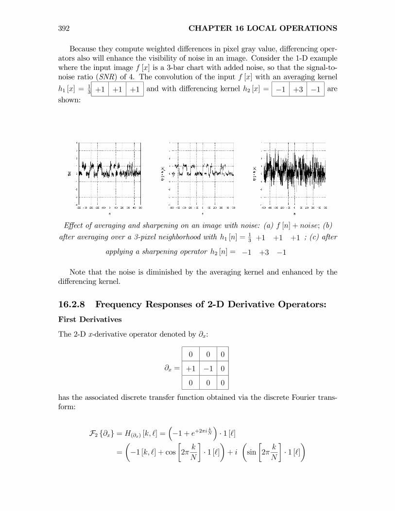
Because they compute weighted differences in pixel gray value, differencing oper-ators also will enhance the visibility of noise in an image. Consider the 1-D examplewhere the input image f [x] is a 3-bar chart with added noise, so that the signal-to-noise ratio (SNR) of 4. The convolution of the input f [x] with an averaging kernel
h1 [x] =13 +1 +1 +1 and with differencing kernel h2 [x] = −1 +3 −1 are
shown:
Effect of averaging and sharpening on an image with noise: (a) f [n] + noise; (b)
after averaging over a 3-pixel neighborhood with h1 [n] =13 +1 +1 +1 ; (c) after
applying a sharpening operator h2 [n] = −1 +3 −1
Note that the noise is diminished by the averaging kernel and enhanced by thedifferencing kernel.
16.2.8 Frequency Responses of 2-D Derivative Operators:
First Derivatives
The 2-D x-derivative operator denoted by ∂x:
∂x =
0 0 0
+1 −1 0
0 0 0
has the associated discrete transfer function obtained via the discrete Fourier trans-form:
F2 {∂x} = H(∂x) [k, ] =³−1 + e+2πi
kN
´· 1 [ ]
=
µ−1 [k, ] + cos
∙2π
k
N
¸· 1 [ ]
¶+ i
µsin
∙2π
k
N
¸· 1 [ ]

16.2 CONVOLUTION 393
The differencing operator in the y-direction and its associated transfer function areobtained by rotating the expressions just derived by +π
2radians. The kernel is:
∂y =
0 0 0
0 −1 0
0 +1 0
The corresponding transfer function is the rotated version of F2 {∂x}:
F2 {∂y} = H(∂y) [k, ] = 1 [k] ·³−1 + e+2πiN
´We can also define 2-D derivatives along angles. We can also define differences alongthe diagonal directions:
∂(θ=+π4 )=
0 0 0
0 −1 0
+1 0 0
∂(θ=+ 3π4 )=
0 0 0
0 −1 0
0 0 +1
The angle in radians has been substituted for the subscript. Again,. the continuousdistance between the elements has been scaled by
√2.
1-D Antisymmetric Differentiation Kernel
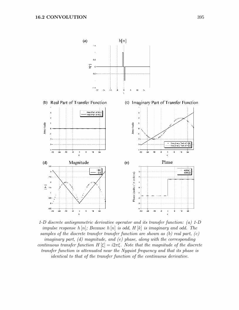
We can also construct a discrete differentiator with odd symmetry by placing thecomponents of the discrete “doublet” at samples n = ±1:
(∂x)2 = +1 0 −1
This impulse response is proportional to the odd part of the original 1-D differentiator.The corresponding transfer function is again easy to evaluate via the appropriatecombination of translation operators. Because (∂x)2 is odd, the real part of thediscrete transfer function is zero, as shown in the figure:

394 CHAPTER 16 LOCAL OPERATIONS
H [k] = exp
∙+2πi
µk
N
¶¸− exp
∙+2πi
µ− k
N
¶¸= 2 i sin
∙2π
k
N
¸|H [k]| = 2
¯̄̄̄sin
∙2π
k
N
¸¯̄̄̄Φ {H [k]} = +π
2
µSGN [k]− δd
∙k +
N
2
¸¶Note that this transfer function evaluated at the Nyquist frequency is:¯̄̄̄
H
∙k = −N
2
¸¯̄̄̄= 2 |sin [−π]| = 0
which means that this differentiator also “blocks” the Nyquist frequency. This maybe seen by convolving (∂x)2 with a sinusoid function that oscillates with a period oftwo samples. Adjacent positive extrema are multiplied by ±1 in the kernel and thuscancel. Also note that the transfer function amplifies lower frequencies more andlarger frequencies less than the continuous transfer function.
16.2 CONVOLUTION 395
1-D discrete antisymmetric derivative operator and its transfer function: (a) 1-Dimpulse response h [n]; Because h [n] is odd, H [k] is imaginary and odd. Thesamples of the discrete transfer transfer function are shown as (b) real part, (c)imaginary part, (d) magnitude, and (e) phase, along with the corresponding
continuous transfer function H [ξ] = i2πξ. Note that the magnitude of the discretetransfer function is attenuated near the Nyquist frequency and that its phase is
identical to that of the transfer function of the continuous derivative.
396 CHAPTER 16 LOCAL OPERATIONS
1-D Second Derivative
The impulse response and transfer function of the continuous second derivative areeasily obtained from the derivative theorem:
h [x] = δ00 [x]
H [ξ] = (2πiξ)2 = −4π2ξ2
Again, different forms of the discrete second derivative may be defined. One formis obtained by differentiating the first derivative operator via discrete convolution oftwo replicas of ∂x. The result is a five-pixel kernel including two null weights:
∂x ∗ ∂x = +1 −1 0 ∗ +1 −1 0
= +1 −2 +1 0 0
The corresponding discrete transfer function is obtained by substituting results fromthe translation operator:
H [k] = e+2πi2kN − 2 e+2πi kN + 1 [k]
= e+2πikN
³e+2πi
kN − 2 + e−2πi
kN
´= 2 e+2πi
kN
µcos
∙2π
k
N
¸− 1
The leading linear phase factor usually is discarded to produce the real-valued andsymmetric discrete transfer function:
H [k] = 2
µcos
∙2π
k
N
¸− 1
Deletion of the linear phase is the same as translation of the original discrete secondderivative kernel by one pixel to the right. The discrete impulse response for thissymmetric discrete kernel is also real valued and symmetric:
h [n] = ∂2x ≡ 0 +1 −2 +1 0 = +1 −2 +1
= δd [n+ 1]− 2δd [n] + δd [n− 1]
and the magnitude and phase of the transfer function are:

16.2 CONVOLUTION 397
|H [k]| = 2µ1− cos
∙2π
k
N
¸
Φ {H [k]} =
⎧⎨⎩−π for k 6= 0
0 for k = 0= π (−1 + δd [k])
as shown in the figure. The amplitude of the discrete transfer function at the Nyquistfrequency is:
H
∙k = −N
2
¸= 2 · (cos [−π]− 1) = −4
while that of the continuous transfer function is −4π2¡−12
¢2= −π2 ∼= −9.87, so the
discrete second derivative does not amplify the amplitude at the Nyquist frequencyas much as the continuous second derivative. The transfer function is a discreteapproximation of the parabola and again approaches the edges of the array to ensuresmooth periodicity.Higher-order discrete derivatives may be derived by repeated discrete convolution
of ∂x, after discarding any linear-phase factors.
1-D Discrete second derivative: (a) Impulse response ∂2x; (b) comparison of discreteand continuous transfer functions.
16.2.9 Laplacian Operator
The Laplacian operator for continuous functions was introduced in the discussion ofelectromagnetism. It is the sum of orthogonal second partial derivatives:
∇2f [x, y] ≡µ
∂2
∂x2+
∂2
∂y2
¶f [x, y]
398 CHAPTER 16 LOCAL OPERATIONS
The associated transfer function is the negative quadratic that evaluates to 0 at DC,which again demonstrates that constant terms are blocked by differentiation:
H [ξ, η] = −4π2¡ξ2 + η2
¢The discrete Laplacian operator is the sum of the orthogonal 2-D second-derivativekernels:
∂2x + ∂2y ≡ ∇2d =0 0 0
+1 −2 +1
0 0 0
+
0 +1 0
0 −2 0
0 +1 0
=
0 +1 0
+1 −4 +1
0 +1 0
The discrete transfer function of this “standard” discrete Laplacian kernel is:
H [k, ] = 2
µcos
∙2π
k
N
¸− 1¶+ 2
µcos
∙2π
N
¸− 1
= 2
µcos
∙2π
k
N
¸+ cos
∙2π
N
¸− 2
The amplitude at the origin is H [k = 0, = 0] = 0 and decays in the horizontal orvertical directions to −6 at the “edge” of the discrete array and to −8 at its corners.
Rotated Laplacian
The sum of the second-derivative kernels along the diagonals creates a rotated versionof the Laplacian, which is “nearly” equivalent to rotating the operator ∇2d by θ = +π
4
radians:
³∂2(+π
4 )+ ∂2(+ 3π
4 )
´= ∇2d
¯̄(+π
4 )=
0 0 +1
0 −2 0
+1 0 0
+
+1 0 0
0 −2 0
0 0 +1
=
+1 0 +1
0 −4 0
+1 0 +1
Derivation of the transfer function is left to the student; its magnitude is zero at theorigin and its maximum negative values are located at the horizontal and verticaledges, but the transfer function zero at the corners.
16.2 CONVOLUTION 399
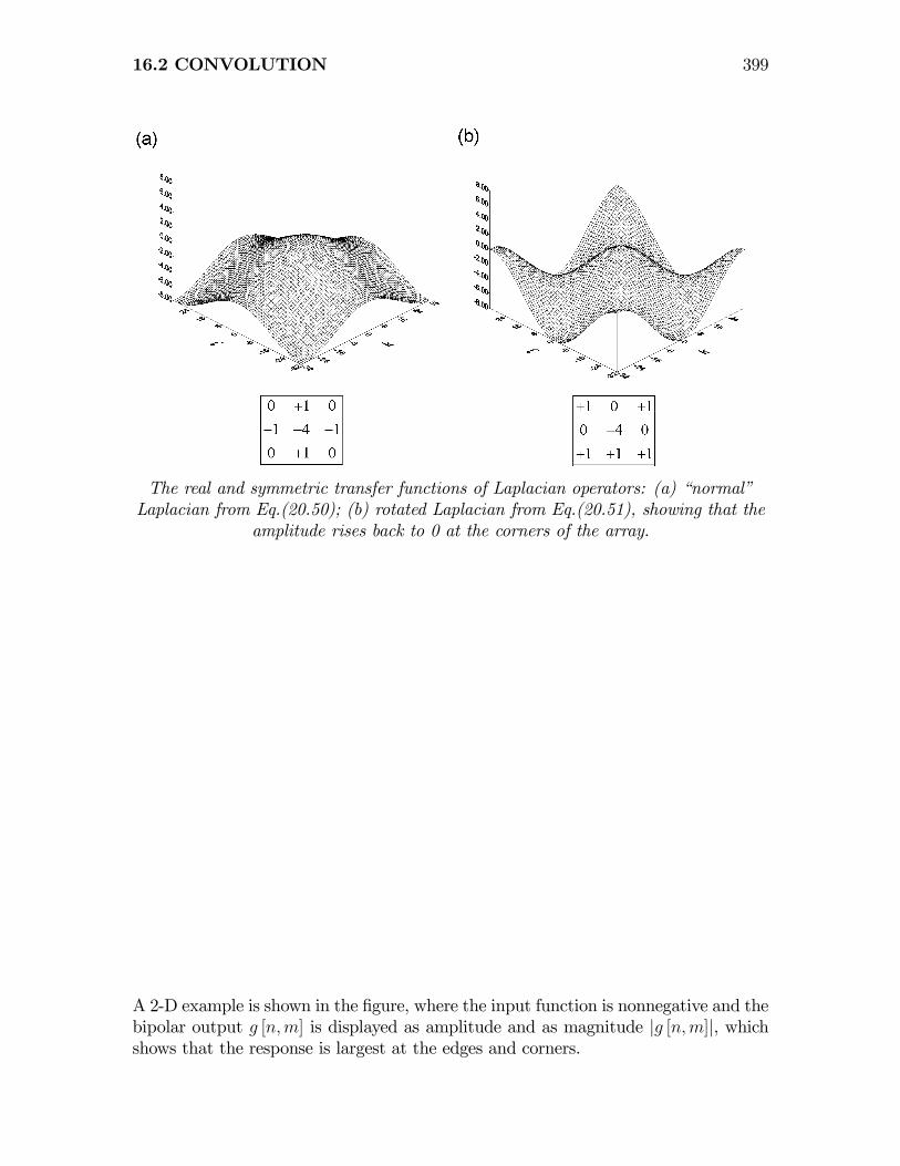
The real and symmetric transfer functions of Laplacian operators: (a) “normal”Laplacian from Eq.(20.50); (b) rotated Laplacian from Eq.(20.51), showing that the
amplitude rises back to 0 at the corners of the array.
A 2-D example is shown in the figure, where the input function is nonnegative and thebipolar output g [n,m] is displayed as amplitude and as magnitude |g [n,m]|, whichshows that the response is largest at the edges and corners.
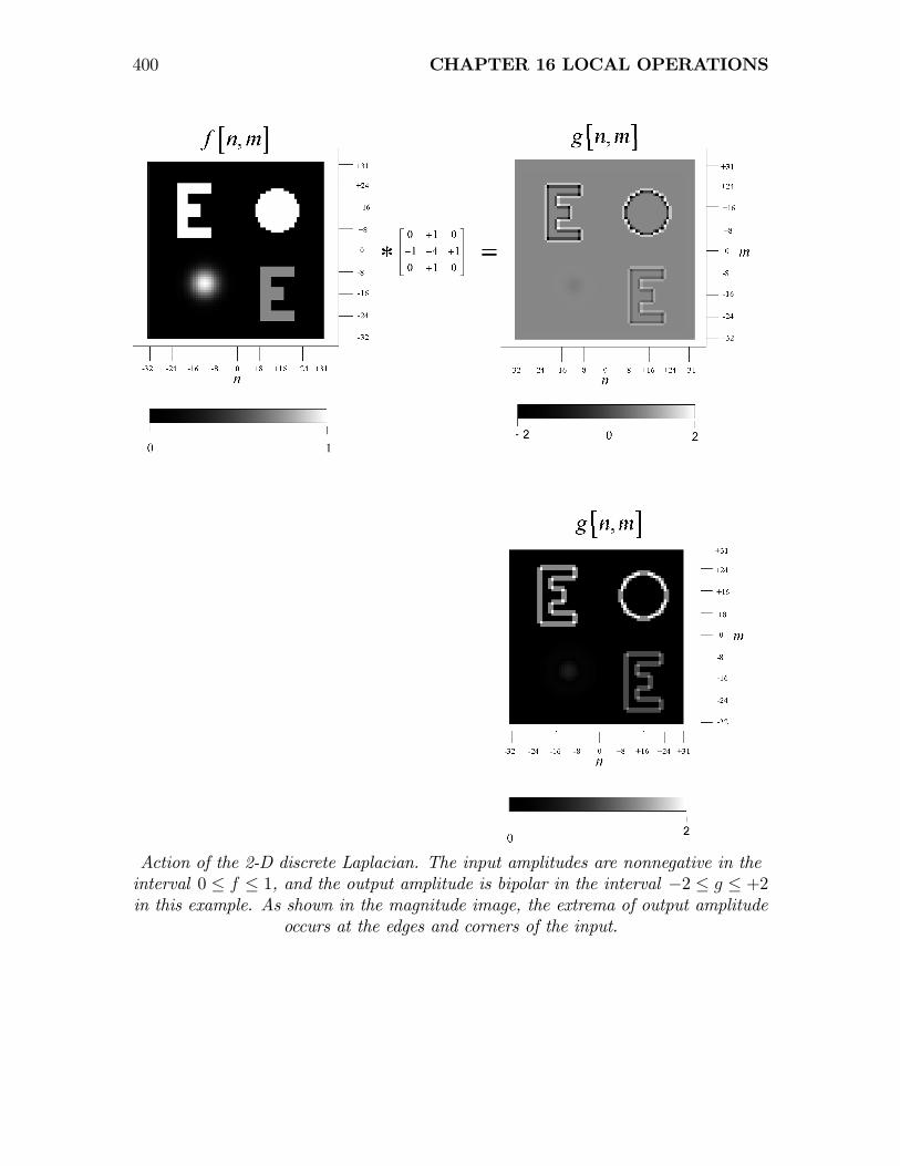
400 CHAPTER 16 LOCAL OPERATIONS
Action of the 2-D discrete Laplacian. The input amplitudes are nonnegative in theinterval 0 ≤ f ≤ 1, and the output amplitude is bipolar in the interval −2 ≤ g ≤ +2in this example. As shown in the magnitude image, the extrema of output amplitude
occurs at the edges and corners of the input.

16.2 CONVOLUTION 401
Isotropic Laplacian:
A commonly used “isotropic” Laplacian is obtained by summing the original androtated Laplacian kernels:
¡∂2x + ∂2y
¢+³∂2(+π
4 )+ ∂2(+3π
4 )
´=
0 +1 0
+1 −4 +1
0 +1 0
+
+1 0 +1
0 −4 0
+1 0 +1
=
+1 +1 +1
+1 −8 +1
+1 +1 +1
The linearity of the DFT ensures that the transfer function of the isotropic Laplacianis the real-valued and symmetric sum of the “normal” and rotated Laplacians.
Generalized Laplacian
The isotropic Laplacian just considered may be written as the difference of a 3 × 3average and a scaled discrete delta function:
+1 +1 +1
+1 −8 +1
+1 +1 +1
=
+1 +1 +1
+1 +1 +1
+1 +1 +1
− 9 ·0 0 0
0 +1 0
0 0 0
which suggests that the Laplacian operator may be generalized to include any operatorthat computes the difference of a scaled original image and replicas that were blurredby some averaging kernel. For example, the impulse response of the averager may bethe 2-D circularly symmetric continuous Gaussian impulse response:
h [x, y] = A exp
∙−π
µx2 + y2
b2
¶¸where the decay parameter b determines the rate at which the values of the kerneldecrease away from the center and the amplitude parameter A often is selected tonormalize the sum of the elements of the kernel to unity, thus ensuring that theprocess computes a weighted average. A normalized discrete approximation of theGaussian kernel with b = 2 ·∆x is:
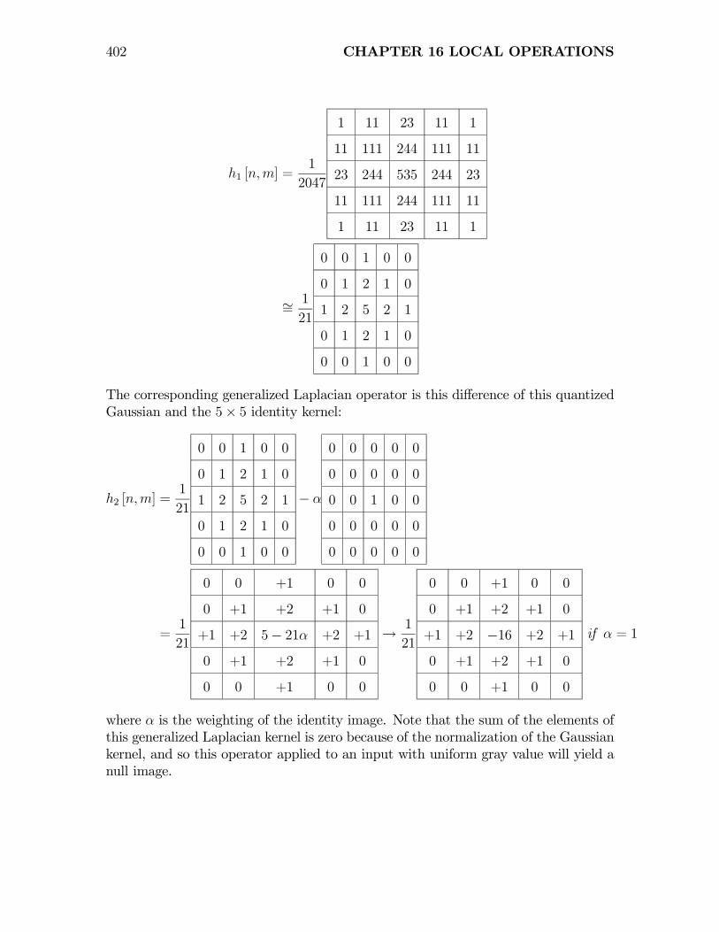
402 CHAPTER 16 LOCAL OPERATIONS
h1 [n,m] =1
2047
1 11 23 11 1
11 111 244 111 11
23 244 535 244 23
11 111 244 111 11
1 11 23 11 1
∼= 1
21
0 0 1 0 0
0 1 2 1 0
1 2 5 2 1
0 1 2 1 0
0 0 1 0 0
The corresponding generalized Laplacian operator is this difference of this quantizedGaussian and the 5× 5 identity kernel:
h2 [n,m] =1
21
0 0 1 0 0
0 1 2 1 0
1 2 5 2 1
0 1 2 1 0
0 0 1 0 0
− α
0 0 0 0 0
0 0 0 0 0
0 0 1 0 0
0 0 0 0 0
0 0 0 0 0
=1
21
0 0 +1 0 0
0 +1 +2 +1 0
+1 +2 5− 21α +2 +1
0 +1 +2 +1 0
0 0 +1 0 0
→ 1
21
0 0 +1 0 0
0 +1 +2 +1 0
+1 +2 −16 +2 +1
0 +1 +2 +1 0
0 0 +1 0 0
if α = 1
where α is the weighting of the identity image. Note that the sum of the elements ofthis generalized Laplacian kernel is zero because of the normalization of the Gaussiankernel, and so this operator applied to an input with uniform gray value will yield anull image.
16.2 CONVOLUTION 403
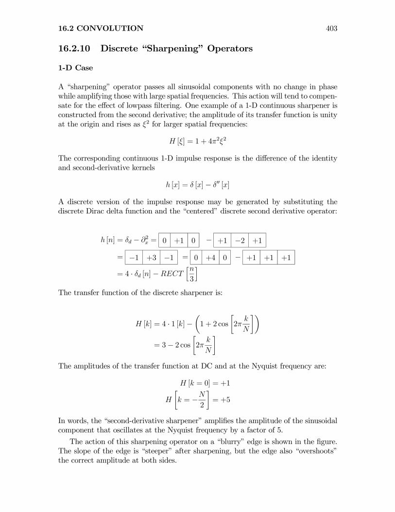
16.2.10 Discrete “Sharpening” Operators
1-D Case
A “sharpening” operator passes all sinusoidal components with no change in phasewhile amplifying those with large spatial frequencies. This action will tend to compen-sate for the effect of lowpass filtering. One example of a 1-D continuous sharpener isconstructed from the second derivative; the amplitude of its transfer function is unityat the origin and rises as ξ2 for larger spatial frequencies:
H [ξ] = 1 + 4π2ξ2
The corresponding continuous 1-D impulse response is the difference of the identityand second-derivative kernels
h [x] = δ [x]− δ00 [x]
A discrete version of the impulse response may be generated by substituting thediscrete Dirac delta function and the “centered” discrete second derivative operator:
h [n] = δd − ∂2x = 0 +1 0 − +1 −2 +1
= −1 +3 −1 = 0 +4 0 − +1 +1 +1
= 4 · δd [n]−RECThn3
iThe transfer function of the discrete sharpener is:
H [k] = 4 · 1 [k]−µ1 + 2 cos
∙2π
k
N
¸¶= 3− 2 cos
∙2π
k
N
¸The amplitudes of the transfer function at DC and at the Nyquist frequency are:
H [k = 0] = +1
H
∙k = −N
2
¸= +5
In words, the “second-derivative sharpener” amplifies the amplitude of the sinusoidalcomponent that oscillates at the Nyquist frequency by a factor of 5.
The action of this sharpening operator on a “blurry” edge is shown in the figure.The slope of the edge is “steeper” after sharpening, but the edge also “overshoots”the correct amplitude at both sides.
404 CHAPTER 16 LOCAL OPERATIONS
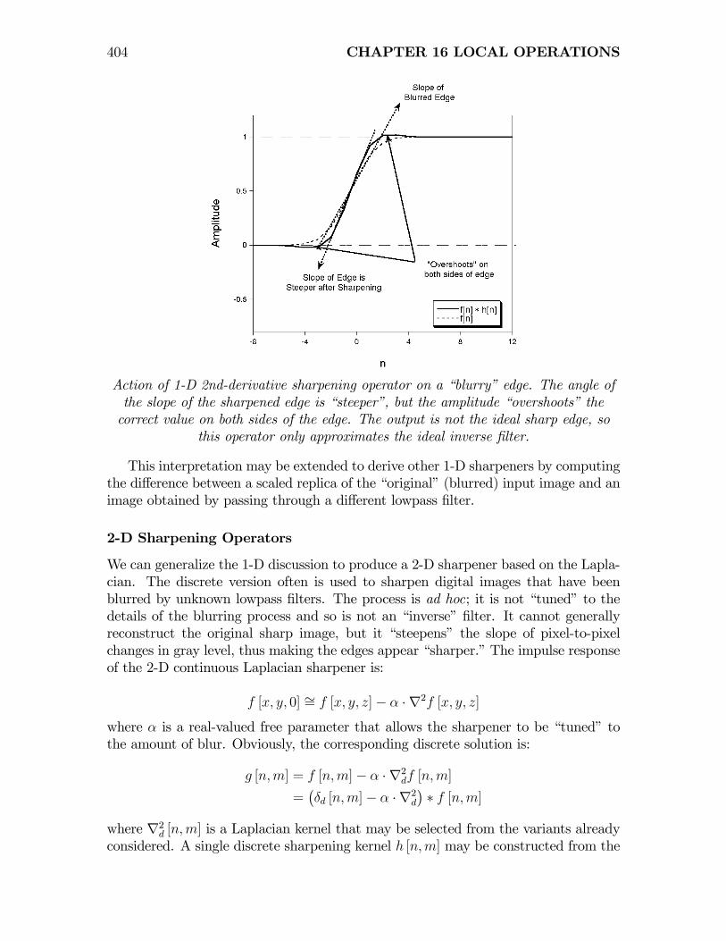
Action of 1-D 2nd-derivative sharpening operator on a “blurry” edge. The angle ofthe slope of the sharpened edge is “steeper”, but the amplitude “overshoots” thecorrect value on both sides of the edge. The output is not the ideal sharp edge, so
this operator only approximates the ideal inverse filter.
This interpretation may be extended to derive other 1-D sharpeners by computingthe difference between a scaled replica of the “original” (blurred) input image and animage obtained by passing through a different lowpass filter.
2-D Sharpening Operators
We can generalize the 1-D discussion to produce a 2-D sharpener based on the Lapla-cian. The discrete version often is used to sharpen digital images that have beenblurred by unknown lowpass filters. The process is ad hoc; it is not “tuned” to thedetails of the blurring process and so is not an “inverse” filter. It cannot generallyreconstruct the original sharp image, but it “steepens” the slope of pixel-to-pixelchanges in gray level, thus making the edges appear “sharper.” The impulse responseof the 2-D continuous Laplacian sharpener is:
f [x, y, 0] ∼= f [x, y, z]− α ·∇2f [x, y, z]where α is a real-valued free parameter that allows the sharpener to be “tuned” tothe amount of blur. Obviously, the corresponding discrete solution is:
g [n,m] = f [n,m]− α ·∇2df [n,m]=¡δd [n,m]− α ·∇2d
¢∗ f [n,m]
where ∇2d [n,m] is a Laplacian kernel that may be selected from the variants alreadyconsidered. A single discrete sharpening kernel h [n,m] may be constructed from the
16.2 CONVOLUTION 405
simplest form for the Laplacian:
h1 [n,m;α] =
0 0 0
0 +1 0
0 0 0
− α ·0 +1 0
+1 −4 +1
0 +1 0
=
0 −α 0
−α 1− 4α −α
0 −α 0
The parameter α may be increased to enhance the sharpening by steepening the slopeof the edge profile and also increasing the “overshoot.” Selection of α = +1 producesa commonly used sharpening kernel:
h1 [n,m;α = +1] =
0 −1 0
−1 +5 −1
0 −1 0
The weights in the kernel sum to unity, which means that the average gray value ofthe image is preserved. In words, this process amplifies differences in gray level ofadjacent pixels while preserving the mean gray value.
The corresponding discrete transfer function for the parameter α is:
H1 [k, ;α] = (1 + 4α)− 2αµcos
∙2π
k
N
¸+ cos
∙2π
N
¸¶In the case α = +1, the resulting transfer function is:
H1 [k, ;α = 1] = 5− 2µcos
∙2π
k
N
¸+ cos
∙2π
N
¸¶which has its maximum amplitude of (H1)max = 9 at the corners of the array.
A sharpening operator also may be derived from the isotropic Laplacian:
h2 [n,m;α] =
−α −α −α
−α 1 + 8α −α
−α −α −α
Again, the sum of the elements in the kernel is unity, ensuring that the average grayvalue of the image is preserved by the action of the sharpener. If the weighting factoris again selected to be unity, the kernel is the difference of a scaled original and a

406 CHAPTER 16 LOCAL OPERATIONS
3× 3 blurred copy:
h2 [n,m; 1] =
−1 −1 −1
−1 +9 −1
−1 −1 −1
=
0 0 0
0 +10 0
0 0 0
−+1 +1 +1
+1 +1 +1
+1 +1 +1
This type of process has been called unsharp masking by photographers. A sandwichof transparencies of the original image and a blurred negative produces a sharpenedimage of the original. This difference of the blurred image and the original is easilyimplemented in a digital system as a single convolution.
An example of 2-D sharpening is shown in the figure. Note the “overshoots” atthe edges in the sharpened image. The factor of +9 ensures that the dynamic rangeof the sharpened image can be as large as from +9 to −8 times the maximum grayvalue, or −2040 ≤ f̂ ≤ +2295 for an 8-bit image. This would only happen for anisolated bright pixel at the maximum surrounded by a neighborhood of black pixels,and vice versa. In actual use, the range of values is considerably smaller. The imagegray values either have to be biased up and rescaled or “clipped” at the maximumand minimum, as was done here.
16.2 CONVOLUTION 407
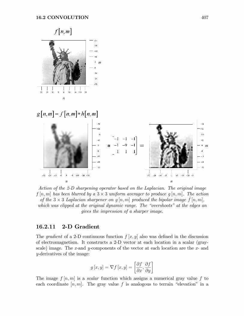
Action of the 2-D sharpening operator based on the Laplacian. The original imagef [n,m] has been blurred by a 3× 3 uniform averager to produce g [n,m]. The actionof the 3× 3 Laplacian sharpener on g [n,m] produced the bipolar image f̂ [n,m],which was clipped at the original dynamic range. The “overshoots” at the edges an
gives the impression of a sharper image.
16.2.11 2-D Gradient
The gradient of a 2-D continuous function f [x, y] also was defined in the discussionof electromagnetism. It constructs a 2-D vector at each location in a scalar (gray-scale) image. The x-and y-components of the vector at each location are the x- andy-derivatives of the image:
g [x, y] = ∇f [x, y] =∙∂f
∂x,∂f
∂y
¸The image f [n,m] is a scalar function which assigns a numerical gray value f toeach coordinate [n,m]. The gray value f is analogous to terrain “elevation” in a
408 CHAPTER 16 LOCAL OPERATIONS
map. This process calculates a vector at each coordinate [x, y] of the scalar imagewhose Cartesian components are ∂f
∂xand ∂f
∂y. Note that the 2-D vector ∇f may be
represented in polar form as magnitude |∇f | and direction Φ {∇f}:
|∇f [x, y]| =
sµ∂f
∂x
¶2+
µ∂f
∂y
¶2
Φ {∇f [n,m]} = tan−1⎡⎣³∂f∂y
´¡∂f∂x
¢⎤⎦
The 2-D vector at each location has the values:
g [n,m] = ∇f [n,m] =
⎡⎣ ∂x ∗ f [n,m]
∂y ∗ f [n,m]
⎤⎦This vector points “uphill” in the direction of the maximum “slope” in gray level.The magnitude |∇f | is the “slope” of the 3-D surface f at pixel [n,m]. The azimuthangle (often called the phase by analogy with complex numbers) of the gradientΦ {∇f [n,m]} is the compass direction toward which the slope points “uphill.”
The discrete version of the gradient magnitude also is a useful operator in digitalimage processing, as it will take on extreme values at edges between objects. Themagnitude of the gradient often is approximated as the sum of the magnitudes of thecomponents:
|∇f [n,m] | =q(∂x ∗ f [n,m])2 + (∂y ∗ f [n,m])2
∼= |∂x ∗ f [n,m]|+ |∂y ∗ f [n,m]|
The gradient is not a linear operator, and thus can neither be evaluated as aconvolution nor described by a transfer function. The largest values of the magnitudeof the gradient correspond to the pixels where the gray value “jumps” by the largestamount, and thus the thresholded magnitude of the gradient may be used to identifysuch pixels. In this way the gradient may be used as an “edge detection operator.”
16.2 CONVOLUTION 409
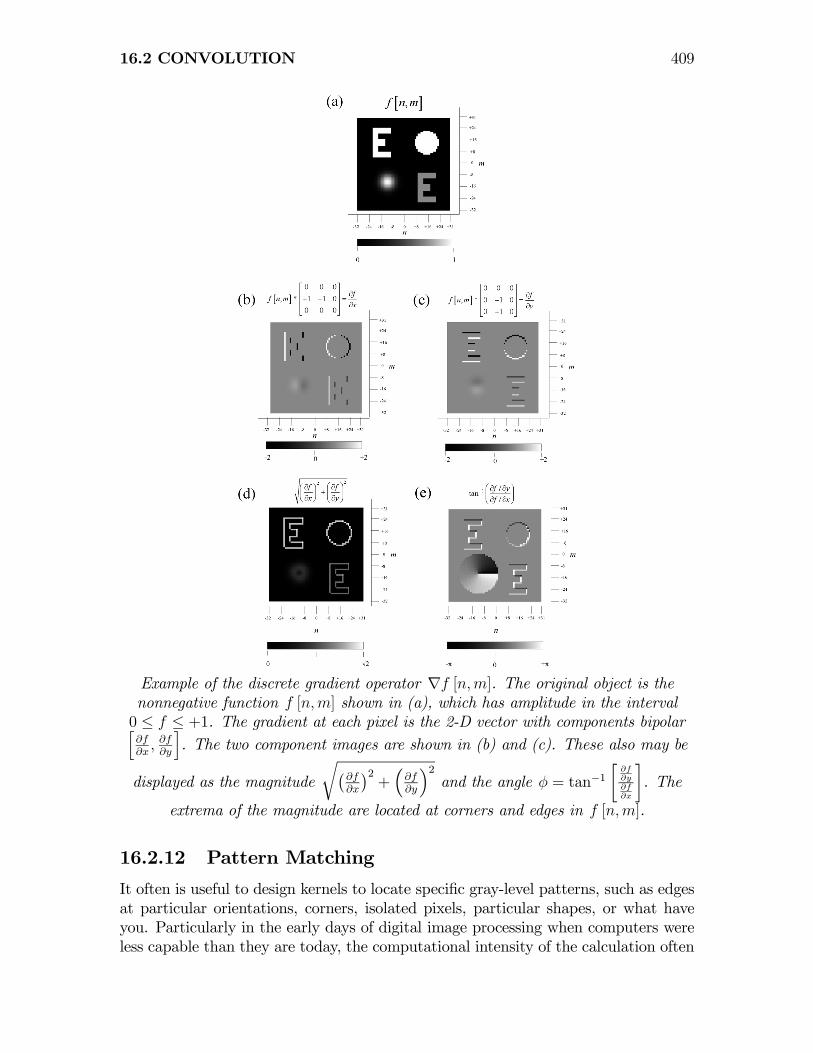
Example of the discrete gradient operator ∇f [n,m]. The original object is thenonnegative function f [n,m] shown in (a), which has amplitude in the interval0 ≤ f ≤ +1. The gradient at each pixel is the 2-D vector with components bipolarh∂f∂x, ∂f∂y
i. The two component images are shown in (b) and (c). These also may be
displayed as the magnitude
r¡∂f∂x
¢2+³∂f∂y
´2and the angle φ = tan−1
∙∂f∂y∂f∂x
¸. The
extrema of the magnitude are located at corners and edges in f [n,m].
16.2.12 Pattern Matching
It often is useful to design kernels to locate specific gray-level patterns, such as edgesat particular orientations, corners, isolated pixels, particular shapes, or what haveyou. Particularly in the early days of digital image processing when computers wereless capable than they are today, the computational intensity of the calculation often

410 CHAPTER 16 LOCAL OPERATIONS
was an important issue. It was desirable to find the least intensive method for commontasks such as pattern detection, which generally meant that the task was performedin the space domain using a small convolution kernel rather than calculating a betterapproximation to the ideal result in the frequency domain. That said, the process ofdesigning and applying a pattern-matching kernel illuminates some of the conceptsand thus is worth some time and effort.
A common technique for pattern matching convolves the input image with a kernelthat is the same size as the “reference” pattern. The process and its limitations willbe illustrated by example. Consider an input image f [n,m] that is composed of tworeplicas of some real-valued nonnegative pattern of gray values, p [n,m] , centered atcoordinates [n1,m1] and [n2,m2] with respective amplitudes A1 and A2. The imagealso includes a bias b · 1 [n,m]:
f [n,m] = A1 · p [n− n1,m−m1] +A2 · p [n− n2,m−m2] + b · 1 [n,m]
The appropriate kernel of the discrete filter is:
m̂ [n,m] = p [−n,−m]
which also is real valued and nonnegative within its region of support. The outputfrom this matched filter autocorrelation of the pattern centered at those coordinates:
g [n,m] = f [n,m] ∗ m̂ [n,m]= A1 · p [n,m]Fp [n,m]|n=n1,m=m1
+A2 · p [n,m]Fp [n,m]|n=n2,m=m2
+ b · (1 [n,m] ∗ p [−n,−m])= A1 · p [n,m]Fp [n,m]|n=n1,m=m1
+A2 · p [n,m]Fp [n,m]|n=n2,m=m2
+ b ·Xn,m
p [n,m]
The last term is the constant output level from the convolution of the bias with thematched filter, which produces the sum of the product of the bias and the weights ateach sample. The spatially varying autocorrelation functions rest on a bias propor-tional to the sum of the gray values p in the pattern. If the output bias is large, itcan reduce the “visibility” of small (but significant) variations in the autocorrelationin exactly the same way as small modulations of a nonnegative sinusoidal functionwith a large bias are difficult to see. It is therefore convenient to construct a matchedfilter kernel whose weights sum to zero. It only requires subtraction of the averagevalue from each sample of the kernel:
m̂ [n,m] = p [−n,−m]− paverage
=⇒Xn,m
m̂ [−n,−m] =Xn,m
m̂ [n,m] = 0
Thus ensuring that the constant bias vanishes. This result determines the strategy
16.2 CONVOLUTION 411
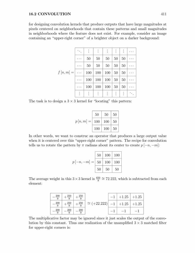
for designing convolution kernels that produce outputs that have large magnitudes atpixels centered on neighborhoods that contain these patterns and small magnitudesin neighborhoods where the feature does not exist. For example, consider an imagecontaining an “upper-right corner” of a brighter object on a darker background:
f [n,m] =
. . ....
......
...... · · ·
· · · 50 50 50 50 50 · · ·
· · · 50 50 50 50 50 · · ·
· · · 100 100 100 50 50 · · ·
· · · 100 100 100 50 50 · · ·
· · · 100 100 100 50 50 · · ·...
......
......
.... . .
The task is to design a 3× 3 kernel for “locating” this pattern:
p [n,m] =
50 50 50
100 100 50
100 100 50
In other words, we want to construc an operator that produces a large output valuewhen it is centered over this “upper-right corner” pattern. The recipe for convolutiontells us to rotate the pattern by π radians about its center to create p [−n,−m]:
p [−n,−m] =50 100 100
50 100 100
50 50 50
The average weight in this 3×3 kernel is 6509∼= 72.222, which is subtracted from each
element:
−2009
+2509
+2509
−2009
+2509
+2509
−2009−200
9−200
9
∼= (+22.222)−1 +1.25 +1.25
−1 +1.25 +1.25
−1 −1 −1
The multiplicative factor may be ignored since it just scales the output of the convo-lution by this constant. Thus one realization of the unamplified 3× 3 matched filterfor upper-right corners is:
412 CHAPTER 16 LOCAL OPERATIONS
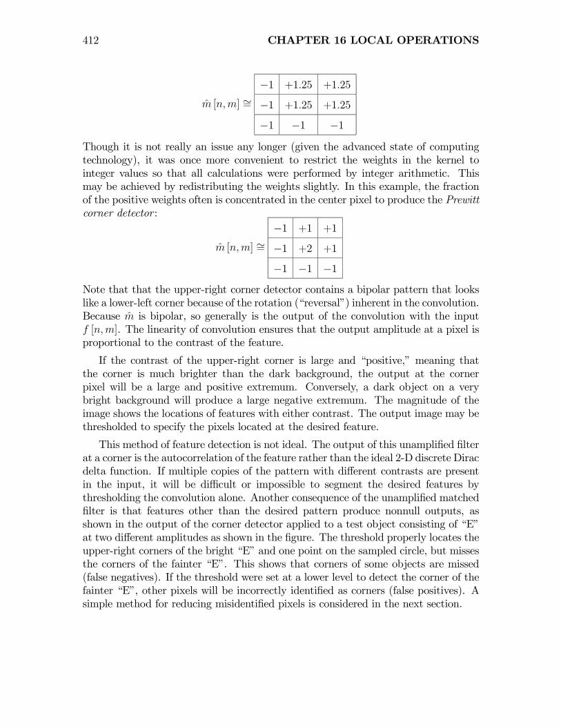
m̂ [n,m] ∼=−1 +1.25 +1.25
−1 +1.25 +1.25
−1 −1 −1
Though it is not really an issue any longer (given the advanced state of computingtechnology), it was once more convenient to restrict the weights in the kernel tointeger values so that all calculations were performed by integer arithmetic. Thismay be achieved by redistributing the weights slightly. In this example, the fractionof the positive weights often is concentrated in the center pixel to produce the Prewittcorner detector :
m̂ [n,m] ∼=−1 +1 +1
−1 +2 +1
−1 −1 −1
Note that that the upper-right corner detector contains a bipolar pattern that lookslike a lower-left corner because of the rotation (“reversal”) inherent in the convolution.Because m̂ is bipolar, so generally is the output of the convolution with the inputf [n,m]. The linearity of convolution ensures that the output amplitude at a pixel isproportional to the contrast of the feature.
If the contrast of the upper-right corner is large and “positive,” meaning thatthe corner is much brighter than the dark background, the output at the cornerpixel will be a large and positive extremum. Conversely, a dark object on a verybright background will produce a large negative extremum. The magnitude of theimage shows the locations of features with either contrast. The output image may bethresholded to specify the pixels located at the desired feature.
This method of feature detection is not ideal. The output of this unamplified filterat a corner is the autocorrelation of the feature rather than the ideal 2-D discrete Diracdelta function. If multiple copies of the pattern with different contrasts are presentin the input, it will be difficult or impossible to segment the desired features bythresholding the convolution alone. Another consequence of the unamplified matchedfilter is that features other than the desired pattern produce nonnull outputs, asshown in the output of the corner detector applied to a test object consisting of “E”at two different amplitudes as shown in the figure. The threshold properly locates theupper-right corners of the bright “E” and one point on the sampled circle, but missesthe corners of the fainter “E”. This shows that corners of some objects are missed(false negatives). If the threshold were set at a lower level to detect the corner of thefainter “E”, other pixels will be incorrectly identified as corners (false positives). Asimple method for reducing misidentified pixels is considered in the next section.

16.2 CONVOLUTION 413
Thresholding to locate features in the image: (a) f [n,m], which is the nonnegativefunction with 0 ≤ f ≤ 1; (b) f [n,m] convolved with the “upper-right cornerdetector”, producing the bipolar output g [n,m] where −5 ≤ g ≤ 4. The largestamplitudes occur at the upper-right corners, as shown in the image thresholded at
level 4, shown in (c) along with the “ghost” of the original image. Thisdemonstrates that the upper-right corners of the high-contrast “E” and of the circle
were detected, but corner of the low-contrast “E” was missed.
414 CHAPTER 16 LOCAL OPERATIONS
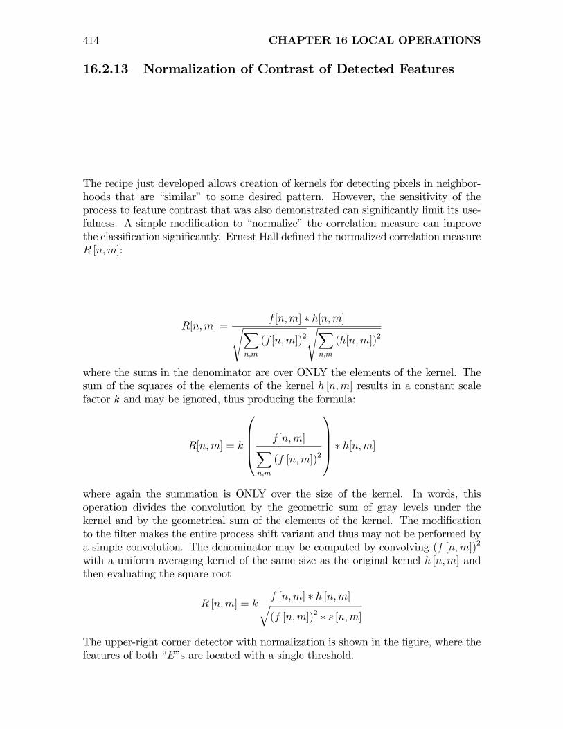
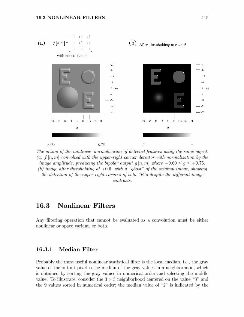
16.2.13 Normalization of Contrast of Detected Features
The recipe just developed allows creation of kernels for detecting pixels in neighbor-hoods that are “similar” to some desired pattern. However, the sensitivity of theprocess to feature contrast that was also demonstrated can significantly limit its use-fulness. A simple modification to “normalize” the correlation measure can improvethe classification significantly. Ernest Hall defined the normalized correlation measureR [n,m]:
R[n,m] =f [n,m] ∗ h[n,m]sX
n,m
(f [n,m])2sX
n,m
(h[n,m])2
where the sums in the denominator are over ONLY the elements of the kernel. Thesum of the squares of the elements of the kernel h [n,m] results in a constant scalefactor k and may be ignored, thus producing the formula:
R[n,m] = k
⎛⎜⎜⎜⎝ f [n,m]Xn,m
(f [n,m])2
⎞⎟⎟⎟⎠ ∗ h[n,m]where again the summation is ONLY over the size of the kernel. In words, thisoperation divides the convolution by the geometric sum of gray levels under thekernel and by the geometrical sum of the elements of the kernel. The modificationto the filter makes the entire process shift variant and thus may not be performed bya simple convolution. The denominator may be computed by convolving (f [n,m])2
with a uniform averaging kernel of the same size as the original kernel h [n,m] andthen evaluating the square root
R [n,m] = kf [n,m] ∗ h [n,m]q(f [n,m])2 ∗ s [n,m]
The upper-right corner detector with normalization is shown in the figure, where thefeatures of both “E”s are located with a single threshold.
16.3 NONLINEAR FILTERS 415
The action of the nonlinear normalization of detected features using the same object:(a) f [n,m] convolved with the upper-right corner detector with normalization by theimage amplitude, producing the bipolar output g [n,m] where −0.60 ≤ g ≤ +0.75;(b) image after thresholding at +0.6, with a “ghost” of the original image, showingthe detection of the upper-right corners of both “E”s despite the different image
contrasts.
16.3 Nonlinear Filters
Any filtering operation that cannot be evaluated as a convolution must be eithernonlinear or space variant, or both.
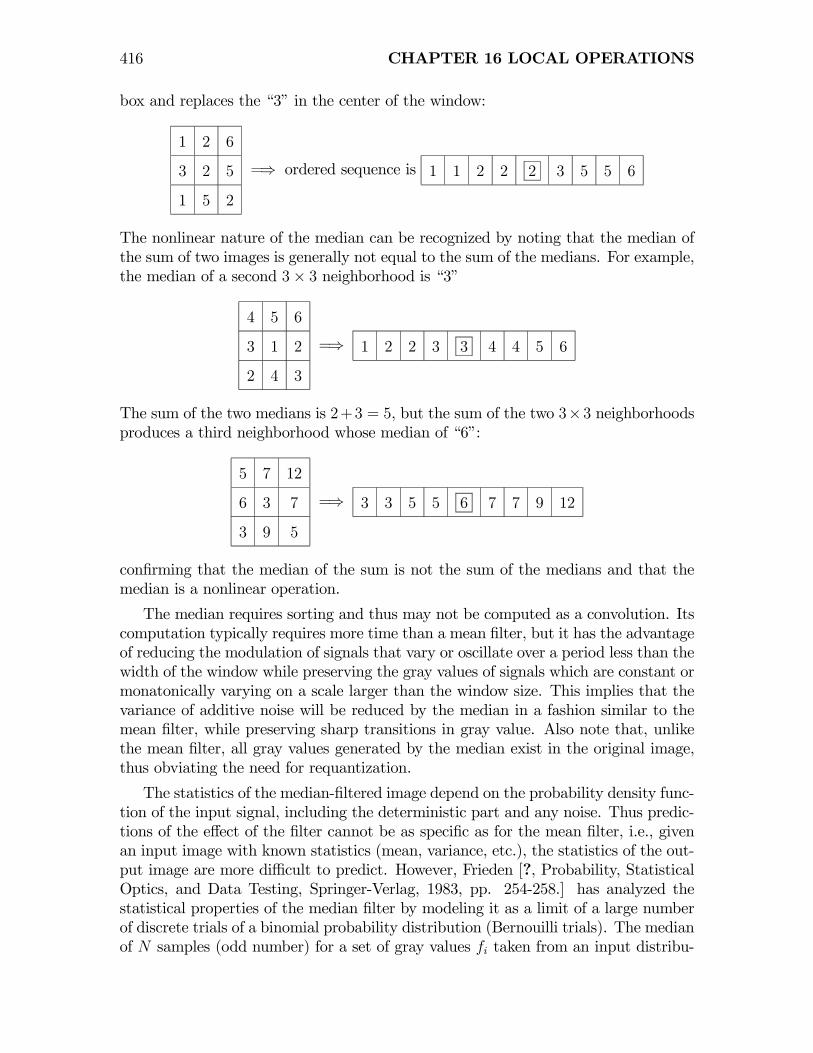
16.3.1 Median Filter
Probably the most useful nonlinear statistical filter is the local median, i.e., the grayvalue of the output pixel is the median of the gray values in a neighborhood, whichis obtained by sorting the gray values in numerical order and selecting the middlevalue. To illustrate, consider the 3× 3 neighborhood centered on the value “3” andthe 9 values sorted in numerical order; the median value of “2” is indicated by the
416 CHAPTER 16 LOCAL OPERATIONS
box and replaces the “3” in the center of the window:
1 2 6
3 2 5
1 5 2
=⇒ ordered sequence is 1 1 2 2 2 3 5 5 6
The nonlinear nature of the median can be recognized by noting that the median ofthe sum of two images is generally not equal to the sum of the medians. For example,the median of a second 3× 3 neighborhood is “3”
4 5 6
3 1 2
2 4 3
=⇒ 1 2 2 3 3 4 4 5 6
The sum of the two medians is 2+3 = 5, but the sum of the two 3×3 neighborhoodsproduces a third neighborhood whose median of “6”:
5 7 12
6 3 7
3 9 5
=⇒ 3 3 5 5 6 7 7 9 12
confirming that the median of the sum is not the sum of the medians and that themedian is a nonlinear operation.
The median requires sorting and thus may not be computed as a convolution. Itscomputation typically requires more time than a mean filter, but it has the advantageof reducing the modulation of signals that vary or oscillate over a period less than thewidth of the window while preserving the gray values of signals which are constant ormonatonically varying on a scale larger than the window size. This implies that thevariance of additive noise will be reduced by the median in a fashion similar to themean filter, while preserving sharp transitions in gray value. Also note that, unlikethe mean filter, all gray values generated by the median exist in the original image,thus obviating the need for requantization.
The statistics of the median-filtered image depend on the probability density func-tion of the input signal, including the deterministic part and any noise. Thus predic-tions of the effect of the filter cannot be as specific as for the mean filter, i.e., givenan input image with known statistics (mean, variance, etc.), the statistics of the out-put image are more difficult to predict. However, Frieden [?, Probability, StatisticalOptics, and Data Testing, Springer-Verlag, 1983, pp. 254-258.] has analyzed thestatistical properties of the median filter by modeling it as a limit of a large numberof discrete trials of a binomial probability distribution (Bernouilli trials). The medianof N samples (odd number) for a set of gray values fi taken from an input distribu-

16.3 NONLINEAR FILTERS 417
tion with probability law (i.e. histogram) pf [x] must be determined. Frieden appliedthe principles of Bernoulli trials to determine the probability density of the medianof several independent sets of numbers. In other words, he sought to determine theprobability that the median of the N numbers {fn} is x by evaluating the medianof many independent such sets of N numbers selected from a known probability dis-tribution pf [x]. Frieden reasoned that, for each placement of the median window, aspecific amplitude fn of the N values is the median if three conditions are satisfied:
1. one of the N numbers satisfies the condition x ≤ fn < x+∆x
2. of the remaining N − 1 numbers, N−12exceed x, and
3. N−12of the remaining numbers are less than x.
The probability of the simultaneous occurence of these three events is the proba-bility density of the output of the median window. For an arbitrary x, any one valuefn must either lie in the interval (x ≤ f < x + ∆x), be larger than x, or less thanx. In other words, each trial has three possible outcomes. These conditions define asequence of Bernoulli trials with three outcomes, which is akin to the task of flippinga “three-sided” coin where the probabilities of the three outcomes are not equal. Inthe more familiar case, the probability that N coin flips with two possible outcomesthat have associated probability p and q will produce m “successes” (say, m heads)is:
PN [m] =N !
(N −m)!m!pm (1− p)N−m
The formula is easy to extend to the more general case of three possible outcomes;the probability that the result yields m1 instances of the first possible outcome (say,“head #1), m2 of the second outcome (“head #2”) and m3 = N − (m1 +m2) of thethird (“tails”) is
PN [m1,m2,m3] = PN [m1,m2, N − (m1 +m2)]
=N !
m1!m2! (N − (m1 +m2))!pm11 pm2
2 pm33
=N !
m1!m2! (N − (m1 +m2))!pm11 pm2
2 (1− (p1 + p2))N−(m1+m2)
where p1, p2, and p3 = 1 − (p1 + p2) are the respective probabilities of the threeoutcomes.When applied to one sample of data, the median filter has three possible outcomes
whose probabilities are known:
1. the sample amplitude may be the median (probability p1),
2. the sample amplitude may be smaller than the median (probability p2), and
3. it may be larger than the median (probability p3).

418 CHAPTER 16 LOCAL OPERATIONS
p1 = P [x ≤ fn ≤ x+∆x] = pf [x]
p2 = P [fn < x] = Cf [x]
p3 = P [fn > x] = 1− Cf [x]
where Cf [x] is the cumulative probability distribution of the continuous probabilitydensity function pf [x]:
Cf [x] =
Z x
−∞pf [α] dα
In this case, the distibutions are continuous (rather than discrete), so the probabilityis the product of the probability density function pmed [x] and the infinitesmal elementdx. We substitute the known probabilities and the known number of occurences ofeach into the Bernoulli formula for three outcomes:
pmed [x] dx =N !¡
N−12
¢! ·¡N−12
¢! · 1!
(Cf [x])N−12 · (1− Cf [x])
N−12 · pf [x] dx
=N !¡¡
N−12
¢!¢2 (Cf [x])
N−12 · [1− Cf [x]]
N−12 pf [x] dx
If the window includes N = 3, 5, or 9 values, the following probability laws for themedian result:
N = 3 =⇒ pmed [x] dx =3!
(1!)2(Cf [x])
1 · (1− Cf [x])N−12 · pf [x] dx
= 6(Cf [x]) · (1− Cf [x]) pf [x] dx
N = 5 =⇒ pmed [x] dx =5!
(2!)2(Cf [x])
2 · [1− Cf [x]]2 pf [x] dx
= 30(Cf [x])2 · (1− Cf [x])
2 pf [x] dx
N = 9 =⇒ pmed [x] dx = 630(Cf [x])4 · (1− Cf [x])
4 pf [x] dx
Example: Median Filter Applied to Uniform Distribution
The statistical properties of the median will now be demonstrated for some simpleexamples of known probabilities. If the original pdf pf [x] is uniform over the interval[0, 1], then it may be written as a rectangle function:
pf [x] = RECT
∙x− 1
2
¸
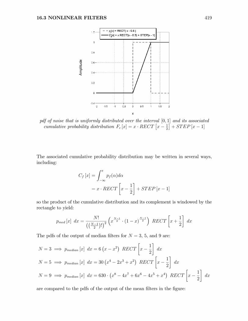
16.3 NONLINEAR FILTERS 419
pdf of noise that is uniformly distributed over the interval [0, 1] and its associatedcumulative probability distribution Fc [x] = x ·RECT
£x− 1
2
¤+ STEP [x− 1]
The associated cumulative probability distribution may be written in several ways,including:
Cf [x] =
Z x
−∞pf(α)dα
= x ·RECT∙x− 1
2
¸+ STEP [x− 1]
so the product of the cumulative distribution and its complement is windowed by therectangle to yield:
pmed [x] dx =N !¡¡
N−12
¢!¢2 ³xN−1
2 · (1− x)N−12
´RECT
∙x+
1
2
¸dx
The pdfs of the output of median filters for N = 3, 5, and 9 are:
N = 3 =⇒ pmedian [x] dx = 6¡x− x2
¢RECT
∙x− 1
2
¸dx
N = 5 =⇒ pmedian [x] dx = 30¡x4 − 2x3 + x2
¢RECT
∙x− 1
2
¸dx
N = 9 =⇒ pmedian [x] dx = 630 ·¡x8 − 4x7 + 6x6 − 4x5 + x4
¢RECT
∙x− 1
2
¸dx
are compared to the pdfs of the output of the mean filters in the figure:
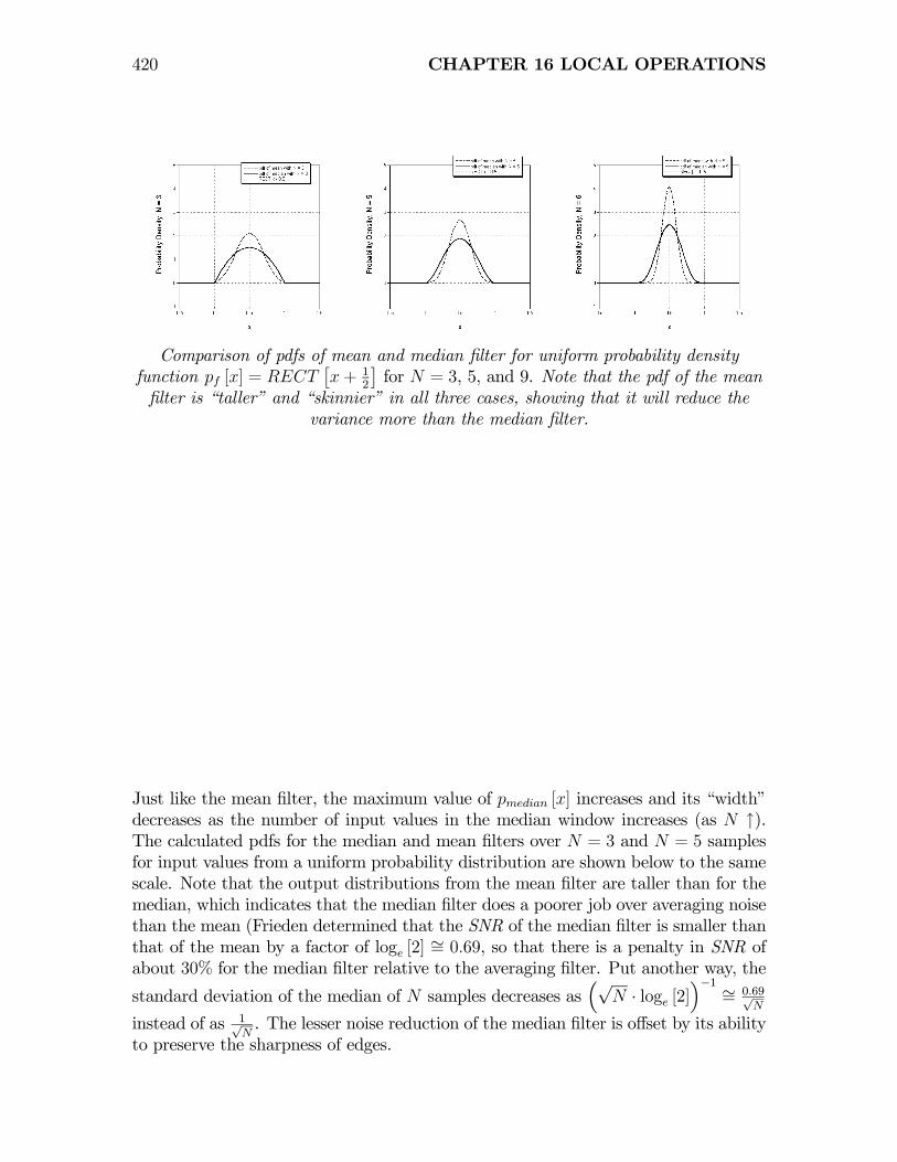
420 CHAPTER 16 LOCAL OPERATIONS
Comparison of pdfs of mean and median filter for uniform probability densityfunction pf [x] = RECT
£x+ 1
2
¤for N = 3, 5, and 9. Note that the pdf of the mean
filter is “taller” and “skinnier” in all three cases, showing that it will reduce thevariance more than the median filter.
Just like the mean filter, the maximum value of pmedian [x] increases and its “width”decreases as the number of input values in the median window increases (as N ↑).The calculated pdfs for the median and mean filters over N = 3 and N = 5 samplesfor input values from a uniform probability distribution are shown below to the samescale. Note that the output distributions from the mean filter are taller than for themedian, which indicates that the median filter does a poorer job over averaging noisethan the mean (Frieden determined that the SNR of the median filter is smaller thanthat of the mean by a factor of loge [2] ∼= 0.69, so that there is a penalty in SNR ofabout 30% for the median filter relative to the averaging filter. Put another way, the
standard deviation of the median of N samples decreases as³√
N · loge [2]´−1 ∼= 0.69√
N
instead of as 1√N. The lesser noise reduction of the median filter is offset by its ability
to preserve the sharpness of edges.

16.3 NONLINEAR FILTERS 421
Comparison of mean and median filter: (a) bitonal object f [m] defined over 1000samples; (b) mean of f [m] over 25 samples, showing reduction in contrast withincreasing frequency; (c) median of f [m] over 25 samples, which is identical to
f [m]; (d) f [m] + n [m], which is uniformly distributed over interval [0, 1]; (e) meanover 25 samples; (f) median over 25 samples. Note that the highest-frequency bars
are better preserved by the median filter.
Example: Median Filter Applied to Gaussian Noise
Probably the most important application of the median filter is to attenuate Gaussiannoise (i.e., the gray values are selected from a normal distribution with zero mean)without blurring edges. The central limit theorem indicates that the statistical char-acter of noise which has been generated by summing random variables from differentdistributions will be Gaussian in character. The probability distribution function isthe Gaussian with mean value µ and variance σ2 normalized to unit area:
pf [x] =1√2πσ2
exp
"−(x− µ)2
2σ2
#
422 CHAPTER 16 LOCAL OPERATIONS
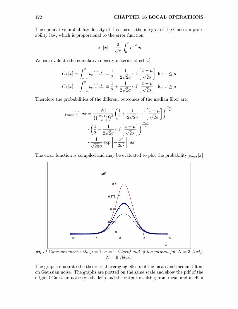
The cumulative probability density of this noise is the integral of the Gaussian prob-ability law, which is proportional to the error function:
erf [x] ≡ 2√π
Z x
0
e−t2
dt
We can evaluate the cumulative density in terms of erf [x]:
Cf [x] =
Z x
−∞pc [x] dx ≡
1
2− 1
2√2σerf
∙x− µ√2σ
¸for x ≤ µ
Cf [x] =
Z x
−∞pc [x] dx ≡
1
2+
1
2√2σerf
∙x− µ√2σ
¸for x ≥ µ
Therefore the probabilities of the different outcomes of the median filter are:
pmed [x] dx =N !¡¡
N−12
¢!¢2 µ12 + 1
2√2σerf
∙x− µ√2σ
¸¶N−12
·µ1
2− 1
2√2σerf
∙x− µ√2σ
¸¶N−12
· 1√2πσ
exp
∙− x2
2σ2
¸dx
The error function is compiled and may be evaluated to plot the probability pmed [x]
1050-5-10
0.5
0.375
0.25
0.125
0
x
x
pdf of Gaussian noise with µ = 1, σ = 2 (black) and of the median for N = 3 (red),N = 9 (blue).
The graphs illustrate the theoretical averaging effects of the mean and median filterson Gaussian noise. The graphs are plotted on the same scale and show the pdf of theoriginal Gaussian noise (on the left) and the output resulting from mean and median
16.3 NONLINEAR FILTERS 423
filtering over 3 pixels (center) and after mean and median filtering over 5 pixels (right).The calculated mean gray value and standard deviation for 2048 samples of filteredGaussian noise yielded the following values:
µin = 0.211
σin = 4.011
µ3 −mean = 0.211
σ3 −mean = 2.355
µ3 −median = 0.225
σ3 −median = 2.745
Effect of Window “Shape” on Median Filter
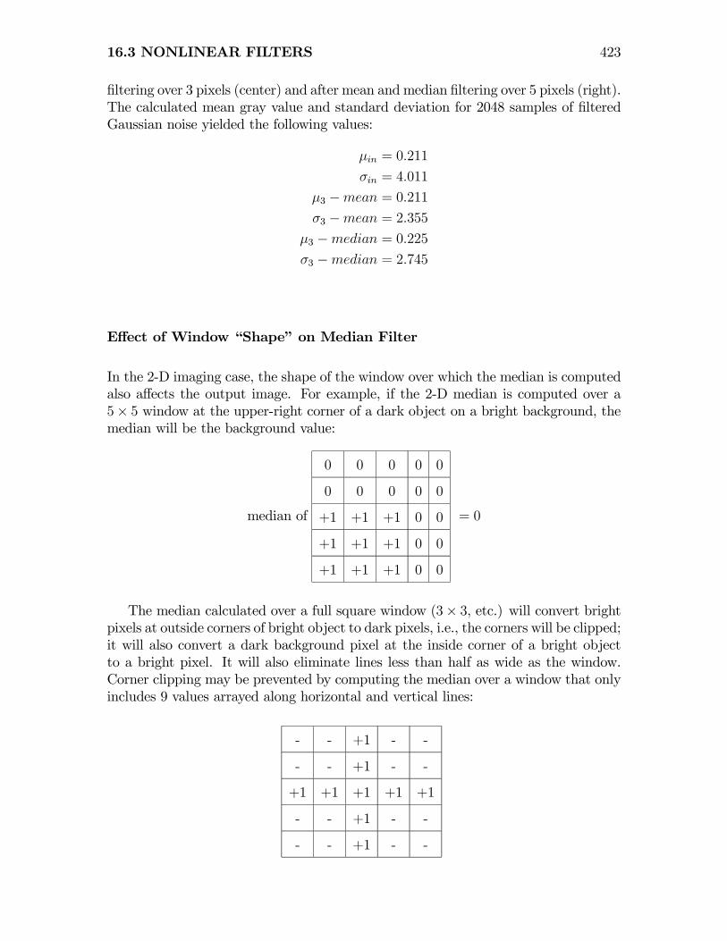
In the 2-D imaging case, the shape of the window over which the median is computedalso affects the output image. For example, if the 2-D median is computed over a5× 5 window at the upper-right corner of a dark object on a bright background, themedian will be the background value:
median of
0 0 0 0 0
0 0 0 0 0
+1 +1 +1 0 0
+1 +1 +1 0 0
+1 +1 +1 0 0
= 0
The median calculated over a full square window (3× 3, etc.) will convert brightpixels at outside corners of bright object to dark pixels, i.e., the corners will be clipped;it will also convert a dark background pixel at the inside corner of a bright objectto a bright pixel. It will also eliminate lines less than half as wide as the window.Corner clipping may be prevented by computing the median over a window that onlyincludes 9 values arrayed along horizontal and vertical lines:
- - +1 - -
- - +1 - -
+1 +1 +1 +1 +1
- - +1 - -
- - +1 - -
424 CHAPTER 16 LOCAL OPERATIONS
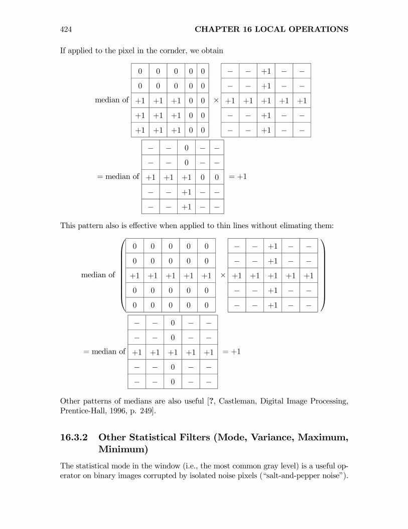
If applied to the pixel in the cornder, we obtain
median of
0 0 0 0 0
0 0 0 0 0
+1 +1 +1 0 0
+1 +1 +1 0 0
+1 +1 +1 0 0
×
− − +1 − −
− − +1 − −
+1 +1 +1 +1 +1
− − +1 − −
− − +1 − −
= median of
− − 0 − −
− − 0 − −
+1 +1 +1 0 0
− − +1 − −
− − +1 − −
= +1
This pattern also is effective when applied to thin lines without elimating them:
median of
⎛⎜⎜⎜⎜⎜⎜⎜⎜⎜⎝
0 0 0 0 0
0 0 0 0 0
+1 +1 +1 +1 +1
0 0 0 0 0
0 0 0 0 0
×
− − +1 − −
− − +1 − −
+1 +1 +1 +1 +1
− − +1 − −
− − +1 − −
⎞⎟⎟⎟⎟⎟⎟⎟⎟⎟⎠
= median of
− − 0 − −
− − 0 − −
+1 +1 +1 +1 +1
− − 0 − −
− − 0 − −
= +1
Other patterns of medians are also useful [?, Castleman, Digital Image Processing,Prentice-Hall, 1996, p. 249].
16.3.2 Other Statistical Filters (Mode, Variance, Maximum,Minimum)
The statistical mode in the window (i.e., the most common gray level) is a useful op-erator on binary images corrupted by isolated noise pixels (“salt-and-pepper noise”).

16.4 ADAPTIVE OPERATORS 425
The mode is found by computing a mini-histogram of pixels within the window andassigning the most common gray level to the center pixel. Rules must be defined iftwo or more gray levels are equally common, and particularly if all levels are popu-lated by a single pixel. If two levels are equally populated, the gray level of centerpixel is usually retained if it is one of those levels; otherwise one of the most commongray levels may be selected at random.The variance filter σ2 and standard deviation filter σ replace the center pixel with
the variance or standard deviation of the pixels in the window, respectively. Thevariance filtering operation is
g [x, y] =X
window
(f [x, y]− µ)2
where µ is the mean value of pixels in the window. The output of a variance orstandard deviation operation will be larger in areas where the image is busy andsmall where the image is smooth. The output of the σ-filter resembles that of theisotropic Laplacian, which computes the difference of the center pixel and the averageof the eight nearest neighbors.The Maximum or Minimum filter obviously replace the gray value in the center
with the highest or lowest value in the window. The MAX filter will dilate brightobjects, while the MIN filter erodes them. These provide the basis for the so-calledmorphological operators. A “dilation” (MAX) followed by an “erosion” (MIN) de-fines the morphological “CLOSE” operation, while the opposite (erosion followed bydilation) is an “OPEN” operation. The “CLOSE” operation fills gaps in lines andremoves isolated dark pixels, while OPENING removes thin lines and isolated brightpixels. These nonlinear operations are useful for object size classification and distancemeasurements
16.4 Adaptive Operators
In applications such as edge enhancement or segmentation, it is often useful to“change”, or “adapt” the operator based on conditions in the image. One exam-ple has already been considered: the nonlinear normalization used while convolvingwith a bipolar convolution kernel. For another example, it is possible to enhancedifferences in the direction of the local gradient (e.g. via a 1-D Laplacian) while aver-aging in the orthogonal direction. In other words, the operator used to enhance theedge information is determined by the output of the gradient operator. As anotherexample, the size of an averaging neighborhood could be varied based on the statistics(e.g., the variance) of gray levels in the neighborhood.In some sense, these adaptive operators resemble cascaded convolutions, but the
resulting operation is not space invariant and may not be desribed by convolutionwith a single kernel. By judicious choice of algorithm, significant improvement ofimage quality may be obtained.
426 CHAPTER 16 LOCAL OPERATIONS
16.5 Convolution Revisited — Bandpass Filters
The parameters of a filter that determine its effect on the image are the size of thekernel and the algebraic sign of its coefficients. Kernels whose elements have thesame algebraic sign are lowpass filters that compute spatial averages and attenuatethe modulation of spatial structure in the image. The larger the kernel, the greater theattenuation. On the other hand, kernels that compute differences of neighboring graylevels will enhance the modulation of spatially varying structure while attenuatingthe brightness of constant areas. Note that the largest number of elements in a kernelwith different algebraic signs is two; the spatial first derivative is an example.We will now construct a hybrid of these two extreme cases that will attenuate the
modulation of image structure that varies more slowly or rapidly than some selectablerate. In other words, the filter will pass a band of spatial frequencies and attenuatethe rest of the spectrum; this is a bandpass filter. The bandpass filter will computedifferences of spatial averages of gray level. For example, consider a 1-D image:
f [n] = 1 +2X
i=0
cos
∙2πn(2i)
128
¸= 1 + cos
∙2πn
∞
¸+ cos
∙2πn
128
¸+ cos
∙2πn
64
¸+ cos
∙2πn
32
¸= 2 + cos
∙2πn
128
¸+ cos
∙2πn
64
¸+ cos
∙2πn
32
¸The spatial frequencies of the cosines are:
ξ0 =1∞ = 0 cycles per sample =⇒ X0 =∞
ξ1 =1128' 7.8 · 10−2 cycles per sample =⇒ X1 = 128 samples
ξ2 =164cycles per sample =⇒ X2 = 64 samples
ξ3 =132cycles per sample =⇒ X3 = 32 samples
This function is periodic over 128 samples, which is a common multiple of all ofthe finite-period cosines. The extreme amplitudes are +5 and +0.2466. Considerconvolution of f [n] with several kernels; the first set are 3-pixel averagers whoseweights sum to unity, therefore preserving the mean gray level of f [n]:
h1[n] = 0 +1 0
h2[n] = +14+12+14
h3[n] = +13+13+13
Obviously, h1[n] is the identity kernel, h2 is a tapered averager that applies moreweight to the center pixel, while h3 is a uniform averager. Based on our experiencewith averaging filters, we know that g1[n] = f [n]∗h1[n]must be identical to f [n], whilethe modulation of the output from h2[n] will be reduced a bit in g2 and somewhat
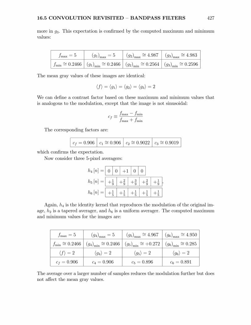
16.5 CONVOLUTION REVISITED — BANDPASS FILTERS 427
more in g3. This expectation is confirmed by the computed maximum and minimumvalues:
fmax = 5 (g1)max = 5 (g2)max∼= 4.987 (g3)max
∼= 4.983
fmin ∼= 0.2466 (g1)min∼= 0.2466 (g2)min
∼= 0.2564 (g3)min∼= 0.2596
The mean gray values of these images are identical:
hfi = hg1i = hg2i = hg3i = 2
We can define a contrast factor based on these maximum and minimum values thatis analogous to the modulation, except that the image is not sinusoidal:
cf ≡fmax − fminfmax + fmin
The corresponding factors are:
cf = 0.906 c1 ∼= 0.906 c2 ∼= 0.9022 c3 ∼= 0.9019
which confirms the expectation.Now consider three 5-pixel averagers:
h4 [n] = 0 0 +1 0 0
h5 [n] = +19+29+39+29+19,
h6 [n] = +15+15+15+15+15
Again, h4 is the identity kernel that reproduces the modulation of the original im-age, h2 is a tapered averager, and h6 is a uniform averager. The computed maximumand minimum values for the images are:
fmax = 5 (g4)max = 5 (g5)max∼= 4.967 (g6)max
∼= 4.950
fmin ∼= 0.2466 (g4)min∼= 0.2466 (g5)min
∼= +0.272 (g6)min∼= 0.285
hfi = 2 hg4i = 2 hg5i = 2 hg6i = 2
cf = 0.906 c4 = 0.906 c5 = 0.896 c6 = 0.891
The average over a larger number of samples reduces the modulation further but doesnot affect the mean gray values.
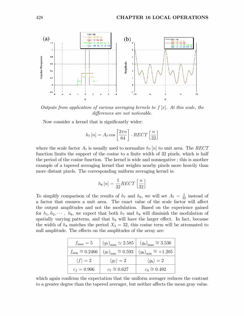
428 CHAPTER 16 LOCAL OPERATIONS
Outputs from application of various averaging kernels to f [x]. At this scale, thedifferences are not noticeable.
Now consider a kernel that is significantly wider:
h7 [n] = A7 cos
∙2πn
64
¸·RECT
h n32
iwhere the scale factor A7 is usually used to normalize h7 [n] to unit area. The RECTfunction limits the support of the cosine to a finite width of 32 pixels, which is halfthe period of the cosine function. The kernel is wide and nonnegative ; this is anotherexample of a tapered averaging kernel that weights nearby pixels more heavily thanmore distant pixels. The corresponding uniform averaging kernel is:
h8 [n] =1
32RECT
h n32
iTo simplify comparison of the results of h7 and h8, we will set A7 = 1
32instead of
a factor that ensures a unit area. The exact value of the scale factor will affectthe output amplitudes and not the modulation. Based on the experience gainedfor h1, h2, · · · , h6, we expect that both h7 and h8 will diminish the modulation ofspatially varying patterns, and that h8 will have the larger effect. In fact, becausethe width of h8 matches the period X3 = 32, this cosine term will be attenuated tonull amplitude. The effects on the amplitudes of the array are:
fmax = 5 (g7)max ' 2.585 (g8)max∼= 3.536
fmin ∼= 0.2466 (g7)min∼= 0.593 (g8)min
∼= +1.205
hfi = 2 hg7i = 2 hg8i = 2
cf = 0.906 c7 ∼= 0.627 c8 ∼= 0.492
which again confirms the expectation that the uniform averager reduces the contrastto a greater degree than the tapered averager, but neither affects the mean gray value.
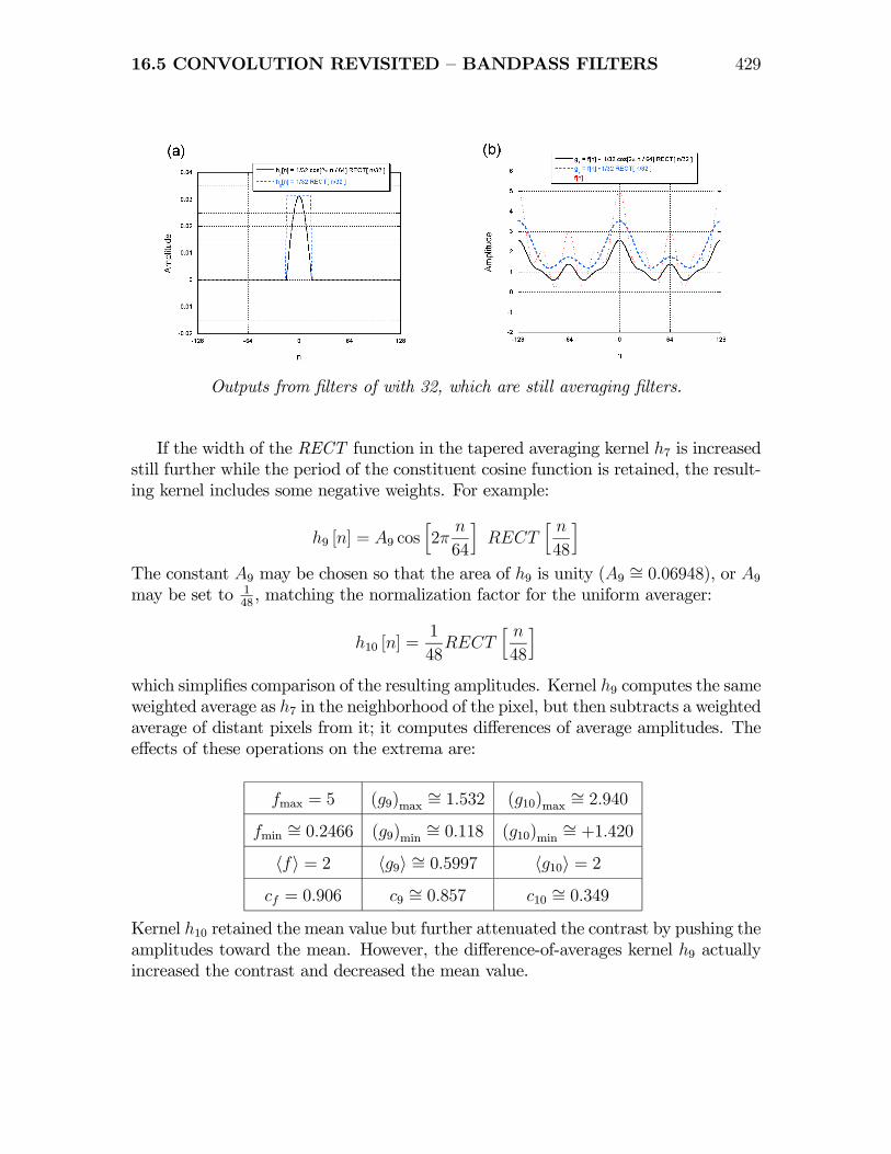
16.5 CONVOLUTION REVISITED — BANDPASS FILTERS 429
Outputs from filters of with 32, which are still averaging filters.
If the width of the RECT function in the tapered averaging kernel h7 is increasedstill further while the period of the constituent cosine function is retained, the result-ing kernel includes some negative weights. For example:
h9 [n] = A9 cosh2π
n
64
iRECT
h n48
iThe constant A9 may be chosen so that the area of h9 is unity (A9 ∼= 0.06948), or A9may be set to 1
48, matching the normalization factor for the uniform averager:
h10 [n] =1
48RECT
h n48
iwhich simplifies comparison of the resulting amplitudes. Kernel h9 computes the sameweighted average as h7 in the neighborhood of the pixel, but then subtracts a weightedaverage of distant pixels from it; it computes differences of average amplitudes. Theeffects of these operations on the extrema are:
fmax = 5 (g9)max∼= 1.532 (g10)max
∼= 2.940
fmin ∼= 0.2466 (g9)min∼= 0.118 (g10)min
∼= +1.420
hfi = 2 hg9i ∼= 0.5997 hg10i = 2
cf = 0.906 c9 ∼= 0.857 c10 ∼= 0.349
Kernel h10 retained the mean value but further attenuated the contrast by pushing theamplitudes toward the mean. However, the difference-of-averages kernel h9 actuallyincreased the contrast and decreased the mean value.
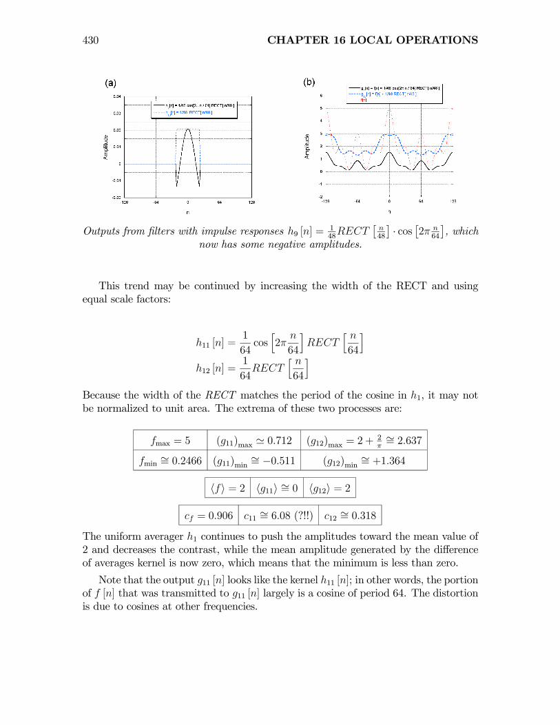
430 CHAPTER 16 LOCAL OPERATIONS
Outputs from filters with impulse responses h9 [n] = 148RECT
£n48
¤· cos
£2π n
64
¤, which
now has some negative amplitudes.
This trend may be continued by increasing the width of the RECT and usingequal scale factors:
h11 [n] =1
64cosh2π
n
64
iRECT
h n64
ih12 [n] =
1
64RECT
h n64
iBecause the width of the RECT matches the period of the cosine in h1, it may notbe normalized to unit area. The extrema of these two processes are:
fmax = 5 (g11)max ' 0.712 (g12)max = 2 +2π∼= 2.637
fmin ∼= 0.2466 (g11)min∼= −0.511 (g12)min
∼= +1.364
hfi = 2 hg11i ∼= 0 hg12i = 2
cf = 0.906 c11 ∼= 6.08 (?!!) c12 ∼= 0.318
The uniform averager h1 continues to push the amplitudes toward the mean value of2 and decreases the contrast, while the mean amplitude generated by the differenceof averages kernel is now zero, which means that the minimum is less than zero.
Note that the output g11 [n] looks like the kernel h11 [n]; in other words, the portionof f [n] that was transmitted to g11 [n] largely is a cosine of period 64. The distortionis due to cosines at other frequencies.

16.5 CONVOLUTION REVISITED — BANDPASS FILTERS 431
Outputs from convolutions with h11 [n] =164RECT
£n64
¤· cos
£2π n
64
¤and
h12 [n] =164RECT
£n64
¤. The bipolar impulse response has zero area and “blocks” the
constant part of the signal.
Now, consider filters whose widths are equal to the period of f [n]:
h13 [n] = cosh2π
n
64
i· 1128
RECTh n
128
ih14 [n] =
1
128RECT
h n
128
i.
The figures of merit for the gray values of these arrays are:
fmax = 5 (g13)max = 0.5 (g14)max = +2
fmin ∼= 0.2466 (g13)min∼= −0.5 (g14)min = +2
hfi = 2 hg13i = 0 hg14i = 2
cf = 0.906 c13 =∞ c14 = 0.0
The output of the bipolar kernel h13 is a sinusoid with period 64 and zero mean, whilethat of the averager h14 is the constant average value of f [n]. Note that the contrastparameter c13 is undefined because fmin = −fmax, while c14 = 0.
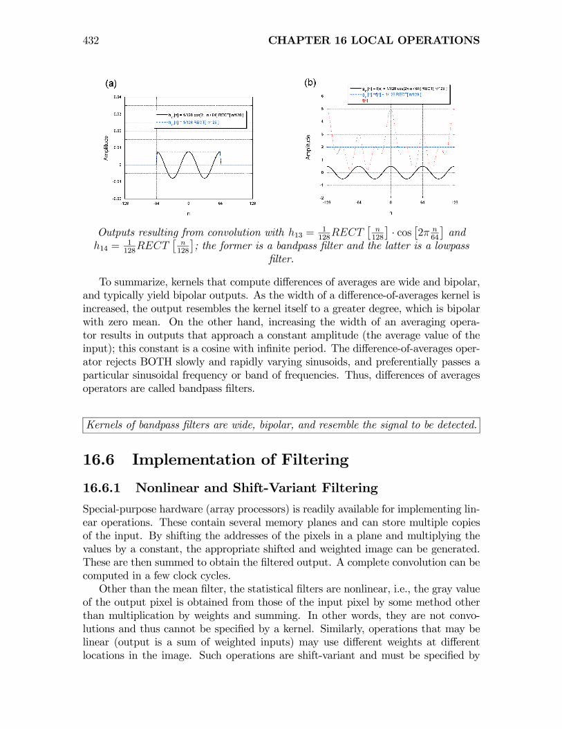
432 CHAPTER 16 LOCAL OPERATIONS
Outputs resulting from convolution with h13 =1128
RECT£
n128
¤· cos
£2π n
64
¤and
h14 =1128
RECT£
n128
¤; the former is a bandpass filter and the latter is a lowpass
filter.
To summarize, kernels that compute differences of averages are wide and bipolar,and typically yield bipolar outputs. As the width of a difference-of-averages kernel isincreased, the output resembles the kernel itself to a greater degree, which is bipolarwith zero mean. On the other hand, increasing the width of an averaging opera-tor results in outputs that approach a constant amplitude (the average value of theinput); this constant is a cosine with infinite period. The difference-of-averages oper-ator rejects BOTH slowly and rapidly varying sinusoids, and preferentially passes aparticular sinusoidal frequency or band of frequencies. Thus, differences of averagesoperators are called bandpass filters.
Kernels of bandpass filters are wide, bipolar, and resemble the signal to be detected.
16.6 Implementation of Filtering
16.6.1 Nonlinear and Shift-Variant Filtering
Special-purpose hardware (array processors) is readily available for implementing lin-ear operations. These contain several memory planes and can store multiple copiesof the input. By shifting the addresses of the pixels in a plane and multiplying thevalues by a constant, the appropriate shifted and weighted image can be generated.These are then summed to obtain the filtered output. A complete convolution can becomputed in a few clock cycles.Other than the mean filter, the statistical filters are nonlinear, i.e., the gray value
of the output pixel is obtained from those of the input pixel by some method otherthan multiplication by weights and summing. In other words, they are not convo-lutions and thus cannot be specified by a kernel. Similarly, operations that may belinear (output is a sum of weighted inputs) may use different weights at differentlocations in the image. Such operations are shift-variant and must be specified by
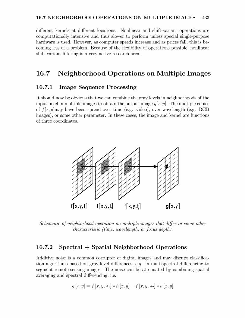
16.7 NEIGHBORHOOD OPERATIONS ON MULTIPLE IMAGES 433
different kernels at different locations. Nonlinear and shift-variant operations arecomputationally intensive and thus slower to perform unless special single-purposehardware is used. However, as computer speeds increase and as prices fall, this is be-coming less of a problem. Because of the flexibility of operations possible, nonlinearshift-variant filtering is a very active research area.
16.7 Neighborhood Operations onMultiple Images
16.7.1 Image Sequence Processing
It should now be obvious that we can combine the gray levels in neighborhoods of theinput pixel in multiple images to obtain the output image g[x, y]. The multiple copiesof f [x, y]may have been spread over time (e.g. video), over wavelength (e.g. RGBimages), or some other parameter. In these cases, the image and kernel are functionsof three coordinates.
Schematic of neighborhood operation on multiple images that differ in some othercharacteristic (time, wavelength, or focus depth).
16.7.2 Spectral + Spatial Neighborhood Operations
Additive noise is a common corrupter of digital images and may disrupt classifica-tion algorithms based on gray-level differences, e.g. in multispectral differencing tosegment remote-sensing images. The noise can be attenuated by combining spatialaveraging and spectral differencing, i.e.
g [x, y] = f [x, y, λ1] ∗ h [x, y]− f [x, y, λ2] ∗ h [x, y]

434 CHAPTER 16 LOCAL OPERATIONS
where
h[x, y] =1
9
+1 +1 +1
+1 +1 +1
+1 +1 +1
Since convolution and subtraction are linear, the order of operations can be inter-changed:
g [x, y] = (f [x, y, λ1]− f [x, y, λ2]) ∗ h [x, y]These can be combined into a single 3-D operation using a 3-D kernel h [x, y, λ]
g[x, y] = f [x, y, λi] ∗ h[x, y, λi]where
h[x, y, λi] = −1
9
+1 +1 +1
+1 +1 +1
+1 +1 +1
,1
9
+1 +1 +1
+1 +1 +1
+1 +1 +1
,1
9
0 0 0
0 0 0
0 0 0