Chapter 16

Integration of Ordinary Differential Equations

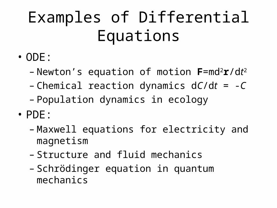
Examples of Differential Equations

• ODE:– Newton’s equation of motion F=md2r/dt2

– Chemical reaction dynamics dC/dt = -C– Population dynamics in ecology

• PDE:– Maxwell equations for electricity and magnetism– Structure and fluid mechanics– Schrödinger equation in quantum mechanics

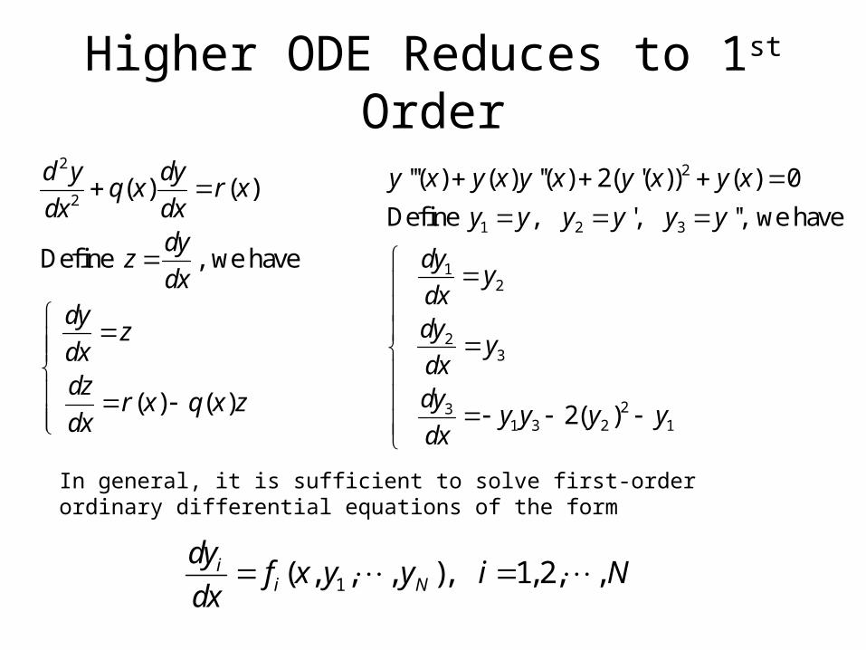
Higher ODE Reduces to 1st Order

2

2( ) ( )

Define , we have

( ) ( )

d y dyq x r x

dx dxdy

zdx

dyz

dxdz

r x q x zdx

2

1 2 3

12

23

231 3 2 1

'''( ) ( ) ''( ) 2( '( )) ( ) 0

Define , ', '', we have

2( )

y x y x y x y x y x

y y y y y y

dyy

dxdy

ydxdy

y y y ydx

In general, it is sufficient to solve first-order ordinary differential equations of the form

1( , , , ), 1, 2, ,ii N

dyf x y y i N

dx

Initial Value Problem

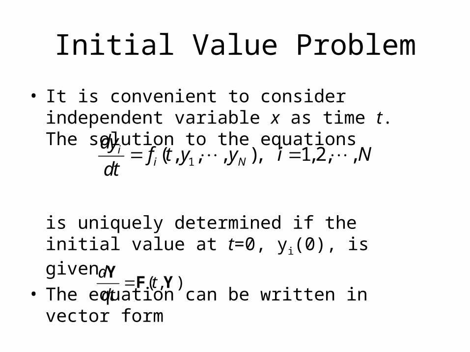
• It is convenient to consider independent variable x as time t. The solution to the equations

is uniquely determined if the initial value at t=0, yi(0), is given.

• The equation can be written in vector form

1( , , , ), 1, 2, ,ii N

dyf t y y i N

dt

( , )d

tdt

Y

F Y

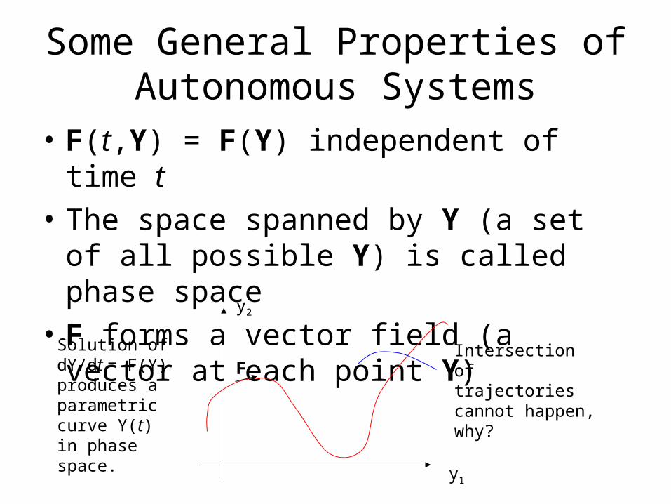
Some General Properties of Autonomous Systems

• F(t,Y) = F(Y) independent of time t

• The space spanned by Y (a set of all possible Y) is called phase space

• F forms a vector field (a vector at each point Y)

y1

y2

Intersection of trajectories cannot happen, why?

Solution of dY/dt = F(Y) produces a parametric curve Y(t) in phase space.

F

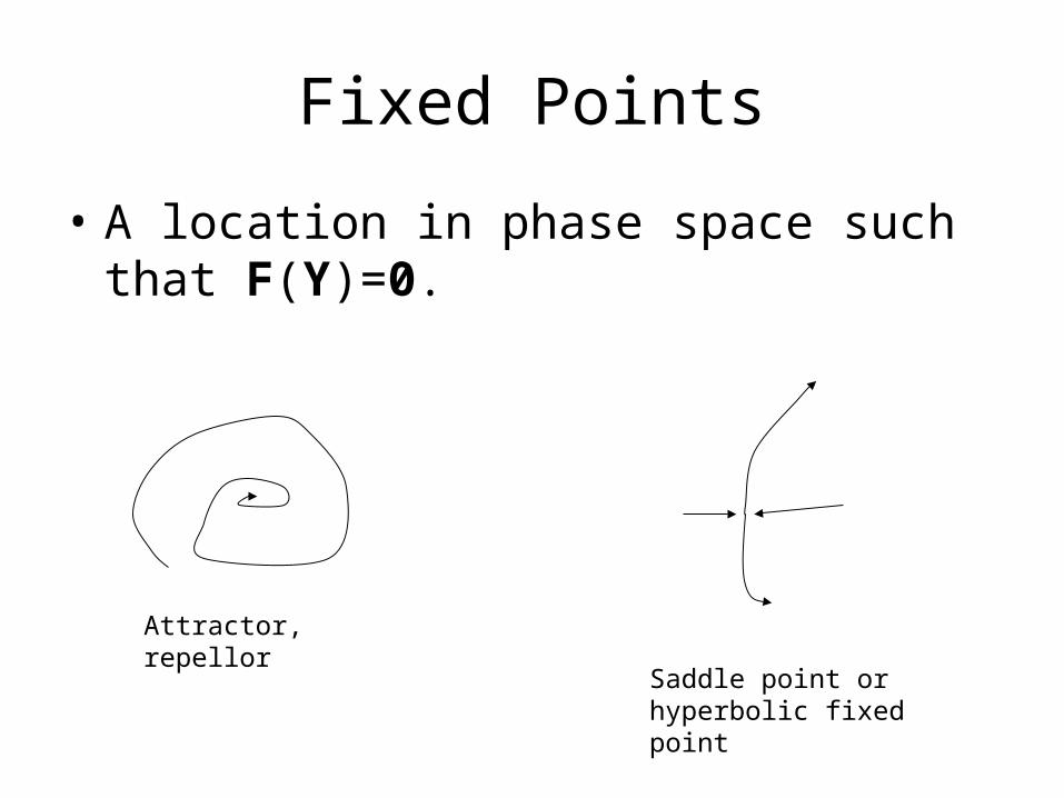
Fixed Points

• A location in phase space such that F(Y)=0.

Attractor, repellor

Saddle point or hyperbolic fixed point

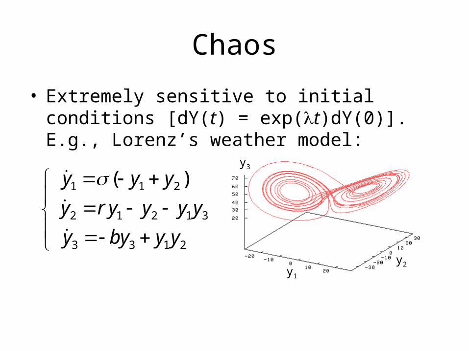
Chaos

• Extremely sensitive to initial conditions [dY(t) = exp(t)dY(0)]. E.g., Lorenz’s weather model:

1 1 2

2 1 2 1 3

3 3 1 2

( )

y y y

y r y y y y

y by y y

y1

y2

y3

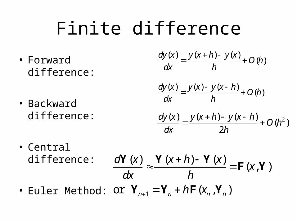
Finite difference

• Forward difference:

• Backward difference:

• Central difference:

• Euler Method:

( ) ( ) ( )( )

dy x y x y x hO h

dx h

( ) ( ) ( )( )

dy x y x h y xO h

dx h

2( ) ( ) ( )( )

2

dy x y x h y x hO h

dx h

1

( ) ( ) ( )( , )

or ( , )n n n n

d x x h xx

dx hh x

Y Y YF Y

Y Y F Y

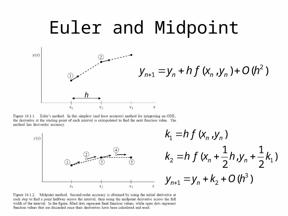
Euler and Midpoint

21 ( , ) ( )n n n ny y h f x y O h

1

2 1

31 2

( , )

1 1( , )

2 2

( )

n n

n n

n n

k h f x y

k h f x h y k

y y k O h

h

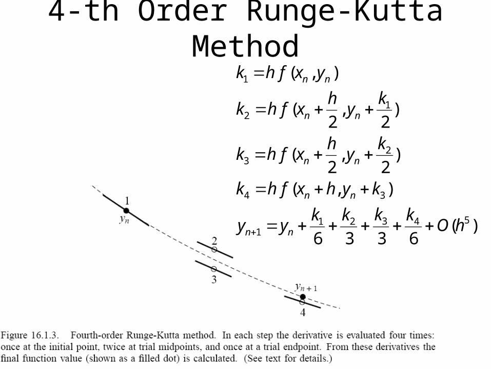
4-th Order Runge-Kutta Method

1

12

23

4 3

531 2 41

( , )

( , )2 2

( , )2 2

( , )

( )6 3 3 6

n n

n n

n n

n n

n n

k h f x y

khk h f x y

khk h f x y

k h f x h y k

kk k ky y O h

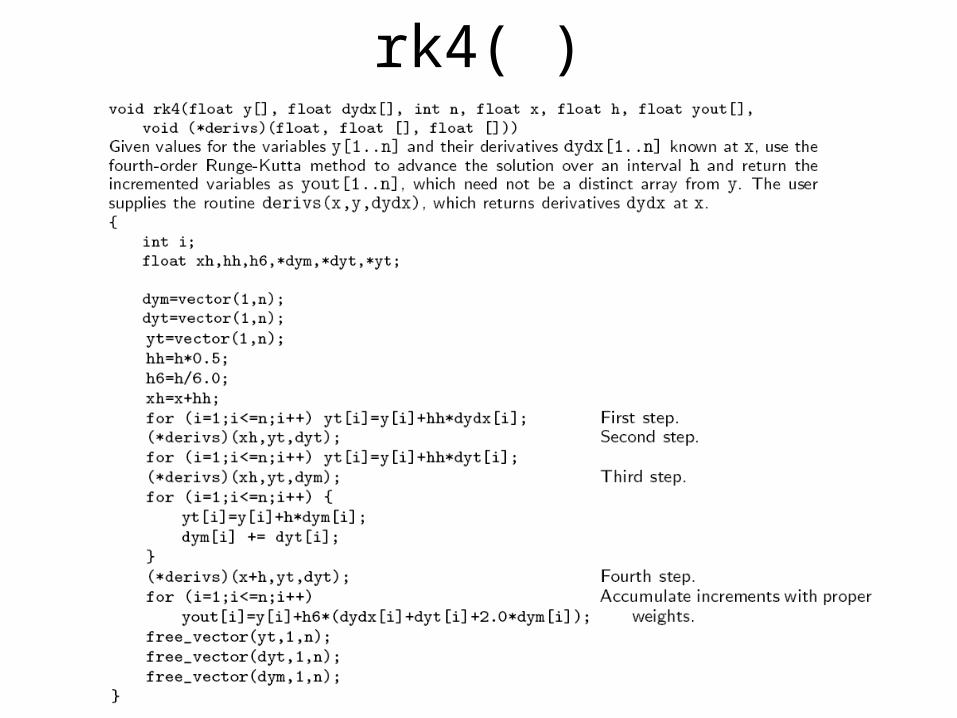
rk4( )

Some General Concepts

• Discretized equations, such as yn+1=yn+hf(xn,yn), is consistent, if as h->0, it approaches the original differential equation

• The error |y(xn+1)-yn+1| =O(hk) in one step from xn to xn+1 is called local truncation error

• The error |y(x)-yn| for some finite x and initial condition y(0) = y0 is the global error

• The method is convergent if the global error goes to zero as h -> 0 and n -> ∞.

Adaptive Stepsize Control

• Estimate local truncation error from difference between one h step and two steps of h/2

• Or difference of 4 and 5-th order Runge-Kutta

• Increase h if error is small than tolerance, decrease h if error is bigger than tolerance. See NR p.721, odeint() for details.

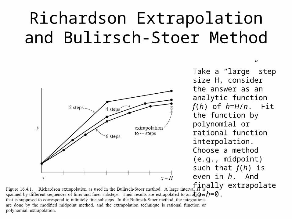
Richardson Extrapolation and Bulirsch-Stoer Method

Take a “large” step size H, consider the answer as an analytic function f(h) of h=H/n. Fit the function by polynomial or rational function interpolation. Choose a method (e.g., midpoint) such that f(h) is even in h. And finally extrapolate to h=0.

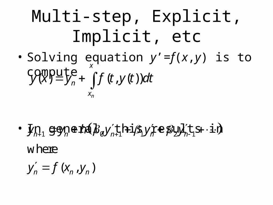
Multi-step, Explicit, Implicit, etc

• Solving equation y’=f(x,y) is to compute

• In general, this results in

( ) ( , ( ))n

x

n

x

y x y f t y t dt

1 0 1 1 2 1

where

( , )

n n n n n

n n n

y y h y y y

y f x y

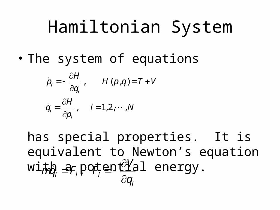
Hamiltonian System

• The system of equations

has special properties. It is equivalent to Newton’s equation with a potential energy.

, ( , )

, 1, 2, ,

ii

ii

Hp H p q T V

q

Hq i N

p

,i i ii

Vmq F F

q

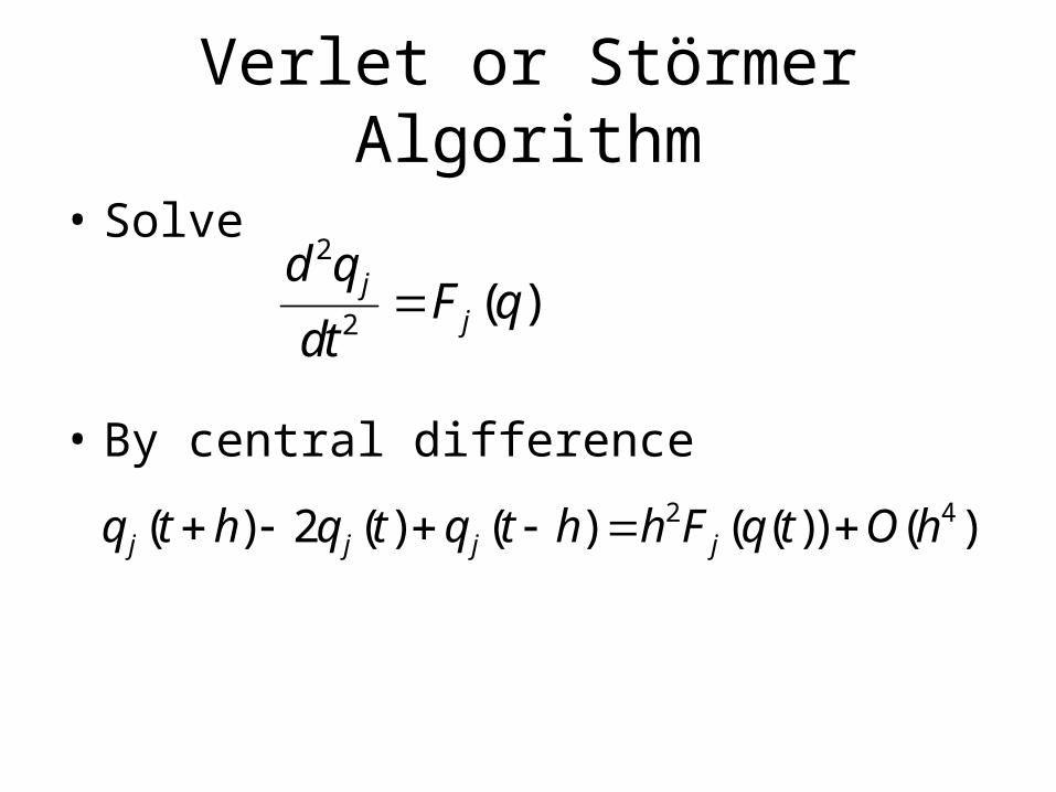
Verlet or Störmer Algorithm

• Solve

• By central difference

2

2( )jj

d qF q

dt

2 4( ) 2 ( ) ( ) ( ( )) ( )j j j jq t h q t q t h h F q t O h

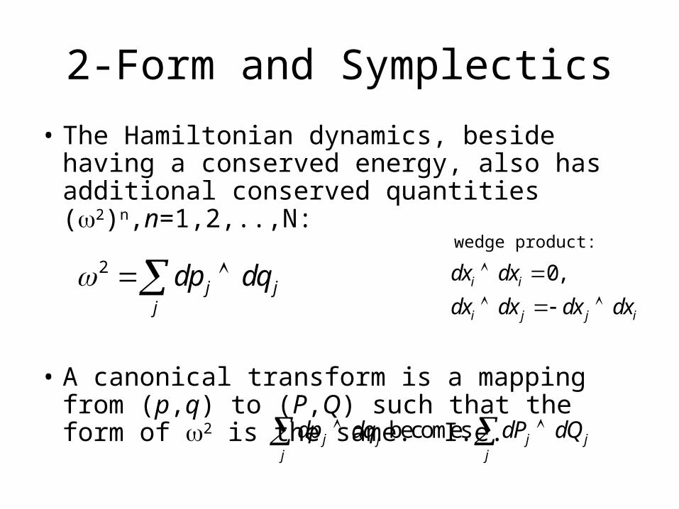
2-Form and Symplectics

• The Hamiltonian dynamics, beside having a conserved energy, also has additional conserved quantities (2)n,n=1,2,..,N:

• A canonical transform is a mapping from (p,q) to (P,Q) such that the form of 2 is the same. I.e.

2j j

j

dp dq 0,i i

i j j i

dx dx

dx dx dx dx

wedge product:

becomesj j j jj j

dp dq dP dQ

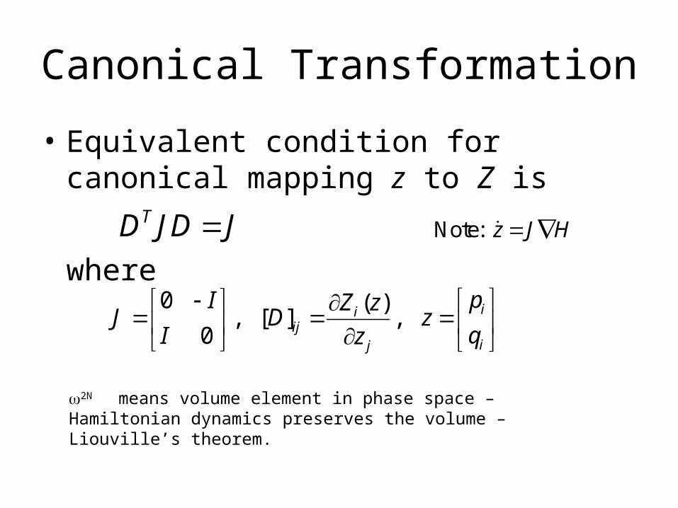
Canonical Transformation

• Equivalent condition for canonical mapping z to Z is

where

TD JD J

0 ( ), [ ] ,

0ii

ijij

pI Z zJ D z

qI z

2N means volume element in phase space – Hamiltonian dynamics preserves the volume – Liouville’s theorem.

Note: z J H

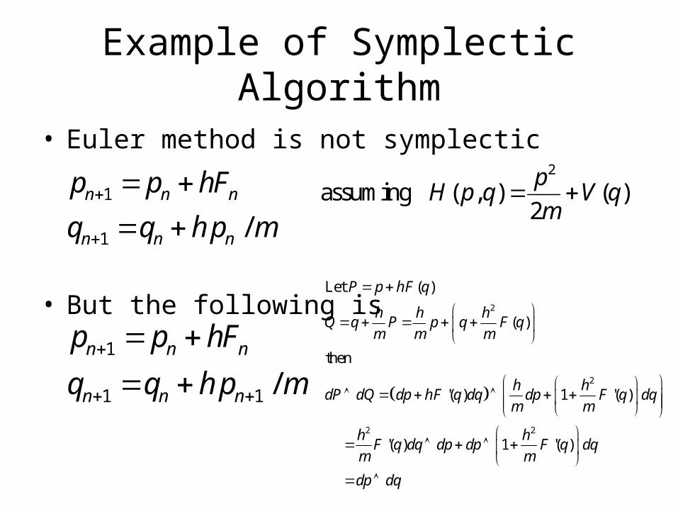
Example of Symplectic Algorithm

• Euler method is not symplectic

• But the following is

1

1 /n n n

n n n

p p hF

q q h p m

1

1 1 /n n n

n n n

p p hF

q q h p m

2

2

2 2

Let ( )

( )

then

'( ) 1 '( )

'( ) 1 '( )

P p hF q

h h hQ q P p q F q

m m m

h hdP dQ dp hF q dq dp F q dq

m m

h hF q dq dp dp F q dq

m m

dp dq

2

assuming ( , ) ( )2

pH p q V q

m

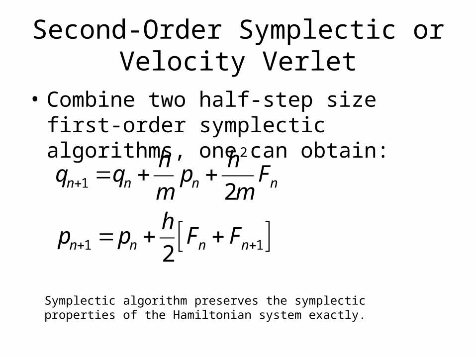
Second-Order Symplectic or Velocity Verlet

• Combine two half-step size first-order symplectic algorithms, one can obtain:

2

1

1 1

2

2

n n n n

n n n n

h hq q p F

m mh

p p F F

Symplectic algorithm preserves the symplectic properties of the Hamiltonian system exactly.

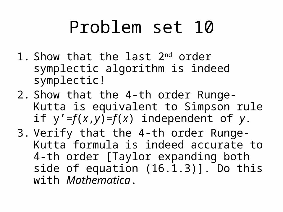
Problem set 10

1. Show that the last 2nd order symplectic algorithm is indeed symplectic!

2. Show that the 4-th order Runge-Kutta is equivalent to Simpson rule if y’=f(x,y)=f(x) independent of y.

3. Verify that the 4-th order Runge-Kutta formula is indeed accurate to 4-th order [Taylor expanding both side of equation (16.1.3)]. Do this with Mathematica.