Chapter 16

General Equilibrium, Efficiency, and Equity

McGraw-Hill/Irwin Copyright © 2008 by The McGraw-Hill Companies, Inc. All Rights Reserved.

Main Topics

The nature of general equilibriumPositive analysis of general equilibriumNormative criteria for evaluating

economic performanceGeneral equilibrium and efficient

exchangeEquity and redistribution

16-2

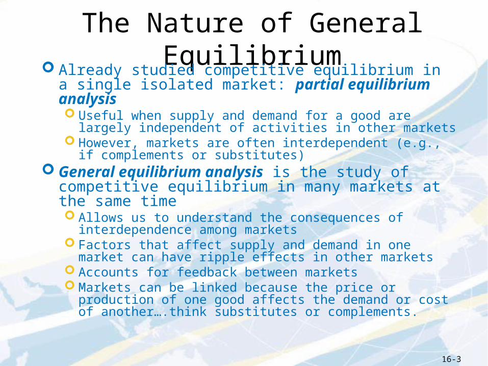
The Nature of General Equilibrium Already studied competitive equilibrium in a single

isolated market: partial equilibrium analysis Useful when supply and demand for a good are largely

independent of activities in other markets However, markets are often interdependent (e.g., if

complements or substitutes) General equilibrium analysis is the study of

competitive equilibrium in many markets at the same time Allows us to understand the consequences of

interdependence among markets Factors that affect supply and demand in one market can have

ripple effects in other markets Accounts for feedback between markets Markets can be linked because the price or production of one

good affects the demand or cost of another….think substitutes or complements.

16-3

Figure 16.1: General Equilibrium

16-4

Above is the general equilibrium in the markets for Pie and Ice cream. Both equilibriums take the other product (and product price) into account in identifying its own product clearing price and quantity.

Positive Analysis ofGeneral Equilibrium

General equilibrium analysis can provide more accurate answers than partial equilibrium analysis does to positive questions

Examine the effects of a sales tax on ice cream Assume pie and ice cream are complements Assume no supply linkages

General equilibrium effects of the tax include: Demand curve for pie shifts downward, so price of pie falls This produces a feedback effect on the ice cream market Effects of the tax ripple back and forth between the markets

Need a new tool to determine the prices that will prevail in both markets in a general equilibrium

16-5

Market-Clearing CurvesFirst step in identifying a general equilibrium is

to find the market-clearing curve for each goodShows the combinations of prices for that good and

related goods that bring supply and demand for the good into balance

Prices of the goods are on the axesFor two goods that are complements, the

market-clearing curves will be downward slopingExample: an increase in the price of pie reduces the

demand for ice cream, which lowers the partial equilibrium price of ice cream

For substitutes, the curves will be upward sloping

16-6

Figure 16.2: A Market-Clearing Curve

16-7

Slide A shows the ice cream curve with 3 different demand curves that correspond to different prices for pie. Slide B is the general equil. market-clearing curve for both products.

Figure 16.2: A Market-Clearing Curve

16-8

Slide A shows the pie curve with 3 different demand curves that correspond to different prices for ice cream. Slide B is the general equil. market-clearing curve for both products.

General Equilibrium inTwo Markets

If a price combination lies on both market-clearing curves, then both markets are in equilibriumThis is a general equilibrium

Find a general equilibrium by plotting both market-clearing curves on the same graph

Horizontal axis shows the price of one good; vertical axis shows the price of the other good

Intersection of the two market-clearing curves reveals the general equilibrium pricesThe two goods markets clear at these prices

16-9

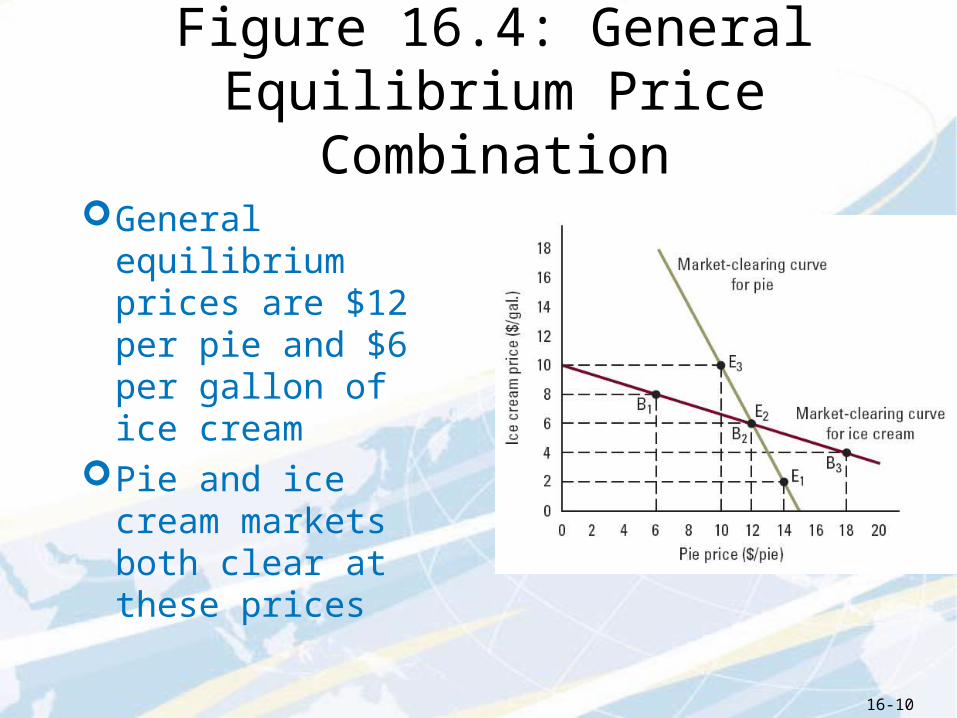
Figure 16.4: General Equilibrium Price Combination

General equilibrium prices are $12 per pie and $6 per gallon of ice cream

Pie and ice cream markets both clear at these prices

16-10

Effects of a Sales Tax:Partial Equilibrium

Continue the ice cream exampleExamine effects of $3 per gallon sales tax on ice

creamBegin from initial equilibrium price of $6 per gallon,

25 million gallonsTax shifts supply curve upward by $3New partial equilibrium is at intersection of the

new supply curve and initial demand curvePrice of pie held constant at $12 per pie

(Consumer) Price of ice cream rises by $1.67 per gallon, less than the amount of the tax

16-11

Effect of a Sales Tax:Gen. Equilibrium

Need new market-clearing curve for ice cream, to find general equilibrium effects of tax

Tax shifts market-clearing curve for ice cream upwardNew curve lies exactly $1.67 above the old oneMagnitude of the shift equals partial equilibrium

effect of the taxLook for intersection of new market-clearing

curve for ice cream and old market-clearing curve for pieShows new general equilibriumPie price is $11 per pie, ice cream price is $8 per

gallonThese prices clear both markets

16-12

Effect of a Sales Tax:Gen. Equilibrium

16-13

Sales Tax Effect : General Equilibrium

As a result of the tax, demand curves for both goods shift

Sales tax on ice cream reduces the price of a pie by $1Because pie and ice cream are complements

Partial equilibrium analysis understates the effect of the tax on the price of ice creamBased on partial anal., ice cream prices rise only by

$1.67, but based on general equil, prices rise by $2.Lower pie price leads to greater demand for ice

creamReinforces pressure for ice cream price to riseGeneral equilibrium analysis accounts for this

feedback; partial equilibrium analysis does not

16-14

Figure 16.6: Effects of a Tax, part 2

16-15

Normative Criteria forEconomic Performance

Economists have clear criteria for measuring efficiency

Equity and fairness are more difficult to determine and evaluate

An allocation of resources is Pareto efficient if it’s impossible to make any consumer better off without hurting someone elseProposed by Italian economist Vilfredo ParetoAssume each person knows what’s best for her

The utility possibility frontier shows the utility levels associated with all efficient allocations of resources

16-16

Figure 16.7: Pareto Efficient Outcomes

Points on the boundary are Pareto efficient

Point A is inefficient

16-17

Equity Equity is harder to define and measure than efficiency

Process-oriented notions of equity focus on the procedures used to arrive at an allocation of resources Focus on what could be chosen instead of what is chosen. Is the free market a fair process?

Outcome-oriented notions focus on whether the process used to allocate resources yields fair results Some focus on the distribution of well-being, e.g., utilitarianism

(equal weight on w-b of every person) Rawlsianism – focus should be on the w-b of the worst-off member

of society Others focus on the distribution of consumption, e.g.,

egalitarianism (equal division of resources to every member of society)

16-18

Social Welfare Functions Economists use social welfare functions to

summarize judgments about resource allocations For each possible allocation, the function assigns a number

that indicates the overall level of social welfare Higher numbers reflect greater social well-being

First, assign utility levels to every consumer using utility functions

Second, apply a function that converts those utilities into social welfare Higher levels of individual utility imply higher levels of social

welfare Can capture concerns for both efficiency and outcome-

oriented notions of equity

NUUUW ,,, WelfareSocial 21 16-19

Figure 16.8: Applying Social Welfare Functions

Indifference curves farther from the origin correspond to higher levels of social welfare

Point A is the best possible outcome

Since Point A is on the utility possibility frontier, it is Pareto efficient

The social welfare function reflects a preference for efficiency

16-20

General Equilibrium inExchange Economies

In an exchange economy, people own and trade goods but no production takes place. This is a starting model to explain the concept.

An endowment is the bundle of goods an individual starts out with before trading

Simple example: Humphrey and Lauren are the only consumers Two goods: food and water Humphrey’s initial endowment is 8 pounds of food and 3 gallons of

water Lauren’s initial endowment is 2 pounds of food and 7 gallons of water

If food sells for $1 per pound and water sells for $1 per gallon this is not a general equilibrium

Supply and demand for the two people match if food costs $2 per pound and water sells for $1 per gallon This is a general equilibrium

16-21

Figure 16.9: General Equilibrium in an Exchange Economy

16-22

The Edgeworth BoxThe Edgeworth box is a diagram that shows

two consumers’ opportunities and choices in a single figureOften used for a simple exchange economyIntroduced by British economist Francis Edgeworth

in 1881Each point describes an allocation of resources

between the two consumersDimensions of the box are determined by the total

amounts of each good available in the economyWhen the economy is in general equilibrium

the points representing the two consumers’ choices after trading coincide

16-23

Equilibrium in an Edgeworth Box

Point A represents initial endowment

Point C is the general equilibrium resource allocation Food costs $2 per pound Water costs $1 per gallon Notice how they coincide. Also, the curves are

opposite due to the inverse nature of the graph.

16-24

The First Welfare Theorem First welfare theorem: in a general equilibrium with

perfect information the allocation of resources is Pareto efficient

Clarifies what Adam Smith mean by the “invisible hand” Use Edgeworth box to understand first welfare theorem

At general equilibrium allocation, two consumers face the same equilibrium prices

Line representing these prices serves as the budget line for both consumers

Impossible to choose an allocation at equilibrium prices, other than equilibrium allocation, that helps one consumer without hurting the other The general equilibrium is Pareto efficient

16-25

Figure 16.11: First Welfare Theorem in an Exchange Economy

16-26

They like points on the budget line equally. But the points of D and E are not as well liked as choosing either of them would

hurt the other party.

Efficiency in Exchange

16-27

Efficiency in Exchange Whenever an allocation is inefficient, there are gains

from trade Whenever an allocation is efficient there are no mutually

beneficial trades The Exchange efficiency condition holds if every pair

of individuals shares the same MRS for every pair of goods Holds as long as consumers’ indifference curves are smooth

and have declining MRS A test for existence of potential gains from trade between

consumers When consumers’ MRS differ, they can both gain by trading

Contract curve shows every efficient allocation of consumption goods in an Edgeworth box Starts at the southwest corner and ends at the northeast

corner Every allocation on the contract curve corresponds to a point

on the utility possibility frontier, and vice versa 16-28

Figure 16.13: Contract Curve

16-29

General Equilibrium andEfficient Production

If add production, competitive equilibria remain Pareto efficient

Exchange efficiency is not enough; production must also be efficient

Two requirements for production efficiency: Input efficiency Output efficiency

Input efficiency: there is no way to increase any firm’s output of one good without decreasing the output of another good Holding constant the total amount of each input used in the

economy Pareto efficiency requires input efficiency

16-30

Input Efficiency Example

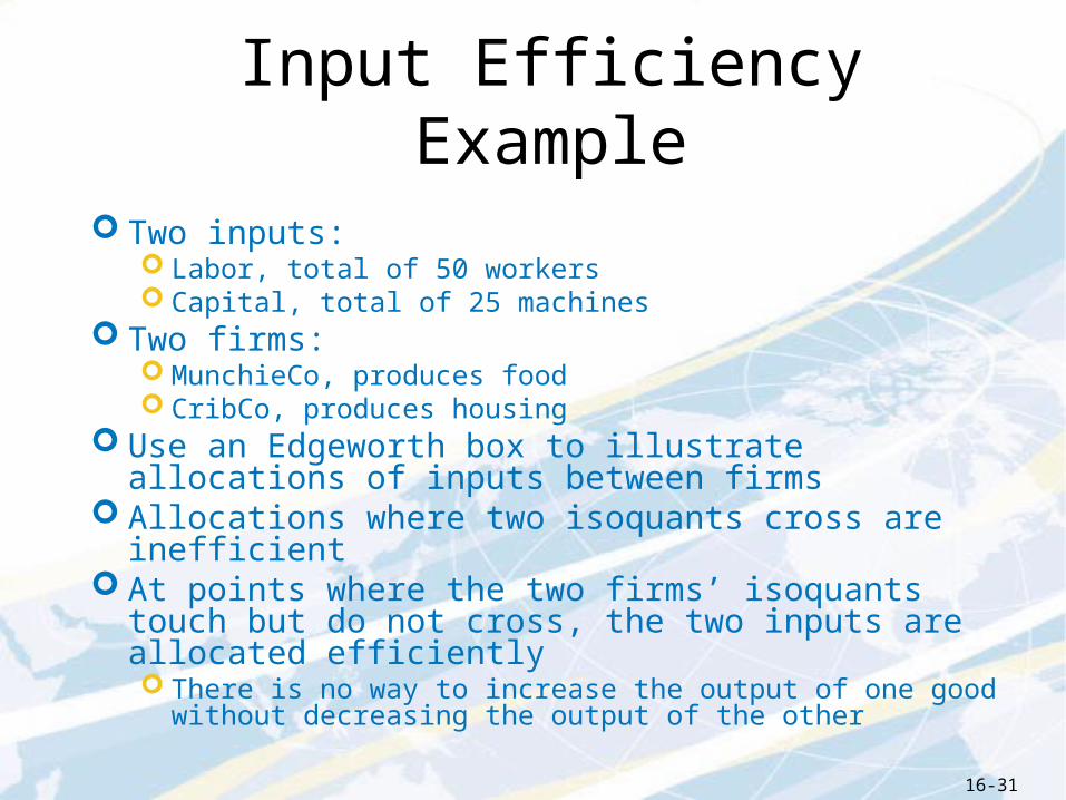
Two inputs: Labor, total of 50 workers Capital, total of 25 machines

Two firms: MunchieCo, produces food CribCo, produces housing

Use an Edgeworth box to illustrate allocations of inputs between firms

Allocations where two isoquants cross are inefficient At points where the two firms’ isoquants touch but do

not cross, the two inputs are allocated efficiently There is no way to increase the output of one good without

decreasing the output of the other

16-31

Figure 16.15: Input Efficiency

16-32

A Condition for Input Efficiency Production contract curve shows every efficient

allocation of inputs between two firms in an Edgeworth box

At efficient allocations, on firm’s MRTSLK is the same as the other’s The firms’ isoquants lie tangent to the same straight line Slope of this line shows the rate at which both firms can

substitute labor for capital without changing their output Input efficiency criterion holds if every pair of firms

shares the MRTS between every pair of inputs As long as the firms’ isoquants are smooth and have declining

MRTS Allocations that satisfy this condition are efficient A test for existence of potential gains from trade between firms

16-33

Production Possibilities Production possibility frontier shows the

combinations of outputs that firms can produce when inputs are allocated efficiently among them Given their technologies and the total inputs available

Relationship between the PPF and the production contract curve is the same as the relationship between the utility possibility frontier and the contract curve

Each input allocation on the production contract curve is associated with a point on the PPF and vice versa

PPF always slopes downward Upward slope would imply that, starting on the frontier, it’s

possible to increase the production of both goods without changing the total amount of any input

But this would mean that the allocation of inputs on the frontier is inefficient and, by definition, the PPF includes only efficient combinations

16-34

Figure 16.16: Production Possibility Frontier

16-35

Marginal Rate of Transformation

Downward slope of the PPF reflects tradeoffs involved in production If we choose to produce more of one good, we must produce less of

another Marginal rate of transformation from good X to good Y is the

additional amount of Y that can be produced by sacrificing one unit of X

At any point on the PPF, the marginal rate of transformation is equal to the slope of a straight line drawn tangent to the frontier at the point, times negative one

Marginal rate of transformation is also related to the firms’ marginal products

Frontier gets steeper moving from left to right Marginal rate of transformation from X to Y rises Reflects decreasing returns to scale in the production technologies

16-36

Output Efficiency Output efficiency means there is no way to make all

consumers better off by shifting production from one good to another Among allocations satisfying exchange efficiency and input

efficiency Achieve input efficiency by picking a point on the

production contract curve Equivalent to picking a point on the PPF

To achieve output efficiency, need to pick the right point

Allocation satisfies the output efficiency condition if, for every pair of goods, every consumer’s MRS equals the marginal rate of transformation

16-37

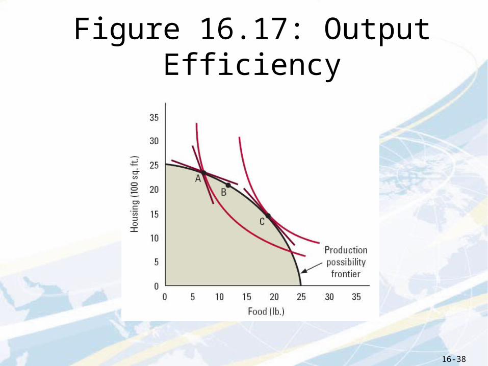
Figure 16.17: Output Efficiency

16-38

Justification for Free Markets Advocates of free markets argue that government

should not play a significant role in overseeing, directing, or conducting economic activity

Doctrine of laissez-faire holds that the government should adopt a “hands off” approach to private commerce

First welfare theorem provides some support for this position Says a perfectly competitive economy would produce an

efficient outcome Opponents have two main reservations

Few economists describe the real economy as perfectly competitive

A market failure is a source of inefficiency in an imperfectly competitive economy

Many people express concerns that free markets can produce inequitable outcomes

16-39

Equity and Redistribution First welfare theorem says that a competitive

equilibrium is Pareto efficient May not convince you that competitive markets are desirable Efficient allocations can be extremely inequitable

Even if the competitive equilibrium is on the contract curve, may be other points on that curve that are more equitable

Second welfare theorem says that every Pareto efficient allocation is a competitive allocation for some initial allocation of resources If the initial allocation of resources heavily favors certain

individuals, the equilibrium will favor them as well In principle, societies can use competitive markets to achieve

both efficiency and equity If society can redistribute the initial allocation of

resources appropriately, then competitive markets will deliver the most equitable Pareto efficient allocation

16-40

Figure 16.20: Second Welfare Theorem

16-41