Chapter 15 The Convection Model for Laminar Flo Chemical reaction engineering...340 Chapter 15 The...

Chapter 15

The Convection Model for Laminar Flow

When a tube or pipe is long enough and the fluid is not very viscous, then the dispersion or tanks-in-series model can be used to represent the flow in these vessels. For a viscous fluid, one has laminar flow with its characteristic parabolic velocity profile. Also, because of the high viscosity there is but slight radial diffusion between faster and slower fluid elements. In the extreme we have the pure convection model. This assumes that each element of fluid slides past its neighbor with no interaction by molecular diffusion. Thus the spread in residence times is caused only by velocity variations. This flow is shown in Fig. 15.1. This chapter deals with this model.

15.1 THE CONVECTION MODEL AND ITS RTD

How to Tell from Theory Which Model to Use

The first question to ask is, "Which model should be used in a given situation?" The following chart, adapted from Ananthakrishnan et al. (1965), tells what regime you are in and which model to use. Just locate the point on Fig. 15.2 which corresponds to the fluid being used (Schmidt number), the flow conditions (Reynolds number), and vessel geometry (LldJ. But be sure to check that your system is not in turbulent flow. Remember that this chart only has meaning if you have laminar flow. In this chart !3lud, is the reciprocal of the Bodenstein number. It measures the flow contribution made by molecular diffusion. It is NOT the axial dispersion number, Dlud, except in the pure diffusion regime. The pure diffusion regime is not a very interesting regime because it represents very very slow flow.

Gases are likely to be in the dispersion regime, not the pure convection regime. Liquids can well be in one regime or another. Very viscous liquids such as polymers are likely to be in the pure convection regime. If your system falls in the no-man's-land between regimes, calculate the reactor behavior based on

340 Chapter 15 The Convection Model for Laminar Flow

Fluid close to the wall moves slowly

I

Fastest flowing fluid element is in the center

Figure 15.1 Flow of fluid according to the convection model.

the two bounding regimes and then try averaging. The numerical solution is impractically complex to use.

Finally, it is very important to use the correct type of model because the RTD curves are completely different for the different regimes. As an illustration, Fig. 15.3 shows RTD curves typical of these regimes.

Lld,

Figure 15.2 Map showing which flow models should be used in any situation.

15.1 The Convection Model and its RTD 341

Pure diffusion gives a pulse output at t = 0 (open-open vessel) \

The dispersion model Pure convection glves gives a more or less

4 the same curve for all & distorted bell s h a ~ e d

flow conditions

0 0.5 1.0

f- Tracer in at t ime zero

Mean for ail three curves

Figure 15.3 Comparison of the RTD of the three models.

How to Tell from Experiment Which Model to Use

The sharpest way of experimentally distinguishing between models comes by noting how a pulse or sloppy input pulse of tracer spreads as it moves downstream in a flow channel. For example, consider the flow, as shown in Fig. 15.4. The dispersion or tanks-in-series models are both stochastic models; thus, from Eq. 13.8 or Eq. 14.3 we see that the variance grows linearly with distance or

The convective model is a deterministic model; thus, the spread of tracer grows linearly with distance, or

Whenever you have measurements of a at 3 points use this test to tell which model to use. Just see if, in Fig. 15.4,

Figure 15.4 The changing spread of a tracer curve tells which model is the right one to use.


Flux introduction Planar introduction

Proportional to velocity; more tracer at centerline very little at the wall

Flux measurement

Evenly distributed across pipe; multiple injectors, a flash of light on photosensitive fluid

Planar measurement

Mixing cup measurement; This could be a through-the-wall catch all the exit fluid. measurement such as with a light In essence this measures u . C meter or radioactivity counter; also

a series of probes (for example conductivity) across the tube. This measures C a t an instant

Figure 15.5 Various ways of introducing and measuring tracer.

Pulse Response Experiment and the E Curve for Laminar Flow in Pipes

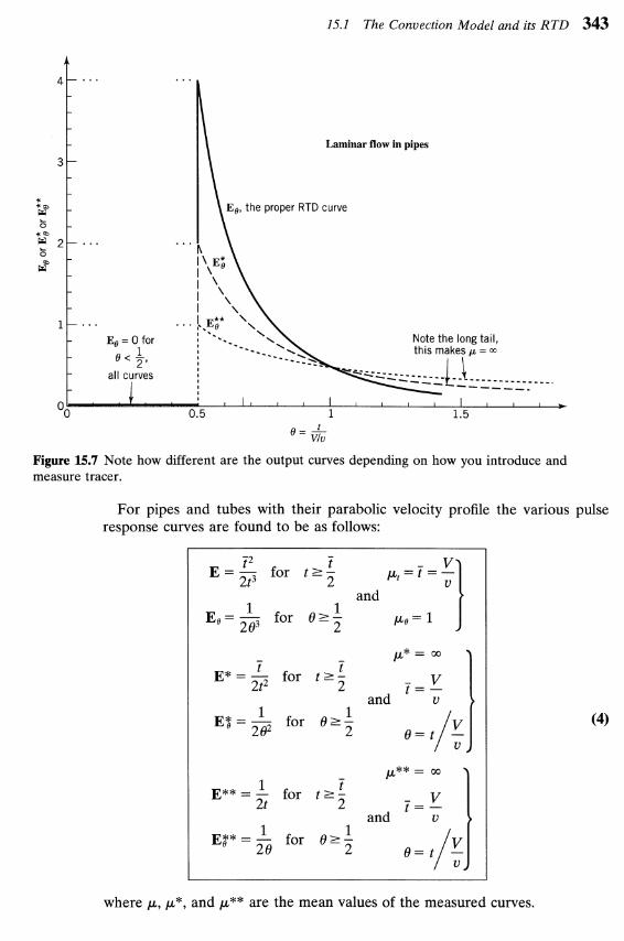
The shape of the response curve is strongly influenced by the way tracer is introduced into the flowing fluid, and how it is measured. You may inject or measure the tracer in two main ways, as shown in Fig. 15.5. We therefore have four combinations of boundary conditions, as shown in Fig. 15.6, each with its own particular E curve. These E curves are shown in Fig. 15.7.

As may be seen in Fig. 15.7, the E, E*, and E** curves are quite different, one from the other.

E is the proper response curve for reactor purposes; it is the curve treated in Chapter 11, and it represents the RTD in the vessel. E* and *E are identical always, so we will call them E* from now on. One correction for the planar boundary condition will transform this curve to the proper RTD. E** requires two corrections-one for entrance, one for exit-to transform it to a proper RTD.

It may be simpler to determine E* or E** rather than E. This is perfectly all right. However, remember to transform these measured tracer curves to the E curve before calling it the RTD. Let us see how to make this transformation.

Flux flux Flux. planar Planar f lux Planar. planar

Figure 15.6 Various combinations of input-output methods.

15.1 The Convection Model and its R T D 343

Figure 15.7 Note how different are the output curves depending on how you introduce and measure tracer.

For pipes and tubes with their parabolic velocity profile the various pulse response curves are found to be as follows:

t2 - t E=- for t z -

2t3 2 and

1 1 E,=- for O r -

2 O3 2

p* = w - t E* = - t

2t2 for t r -

2 and

1 E? = - 1 2 O2

for 132 - 2

p** = CO

1 E** = - t 2t

for t r - 2

and 1 E$* = - 1

2 O for O r -

2

where p, p*, and p** are the mean values of the measured curves.


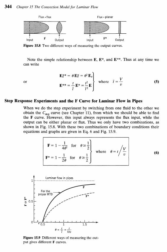
Flux flux Flux planar

Figure 15.8 Two different ways of measuring the output curves.

Note the simple relationship between E, E*, and E*". Thus at any time we can write

E$* = 8 E$ = O2 EB v

where 7 = - v

t t2

Step Response Experiments and the F Curve for Laminar Flow in Pipes

When we do the step experiment by switching from one fluid to the other we obtain the C,,,, curve (see Chapter ll), from which we should be able to find the F curve. However, this input always represents the flux input, while the output can be either planar or flux. Thus we only have two combinations, as shown in Fig. 15.8. With these two combinations of boundary conditions their equations and graphs are given in Eq. 6 and Fig. 15.9.

1 F=l-- for 4 O2

where 8 = t 1

F*= I-- for 8 2 - 2 8

t Laminar flow in pipes 1 -------------....-.....---....-.--....

,g=&=L t V/u

Figure 15.9 Different ways of measuring the output gives different F curves.

15.2 Chemical Conversion in Laminar Flow Reactors 345

Also each F curve is related to its corresponding E curve. Thus at any time t, or 6,

01 * F* = 1; E: dl = 1 E0 do and E: = or E: =@I (7) 0 do 0,

The relationship is similar between E and F.

E Curves for Non-newtonians and for Non-circular Channels

Since plastics and nonnewtonians are often very viscous they usually should be treated by the convective model of this chapter. The E, E*, and E** curves for various situations besides newtonian fluids in circular pipes have been developed, for example,

for power law fluids for Bingham plastics

E curves have also been developed

for falling films for flow between parallel plates where line measurements are made rather than across the whole vessel cross section.

These E equations and corresponding charts plus sources to various other analy- ses can be found in Levenspiel, (1996).

15.2 CHEMICAL CONVERSION IN LAMINAR FLOW REACTORS

Single n-th Order Reactions

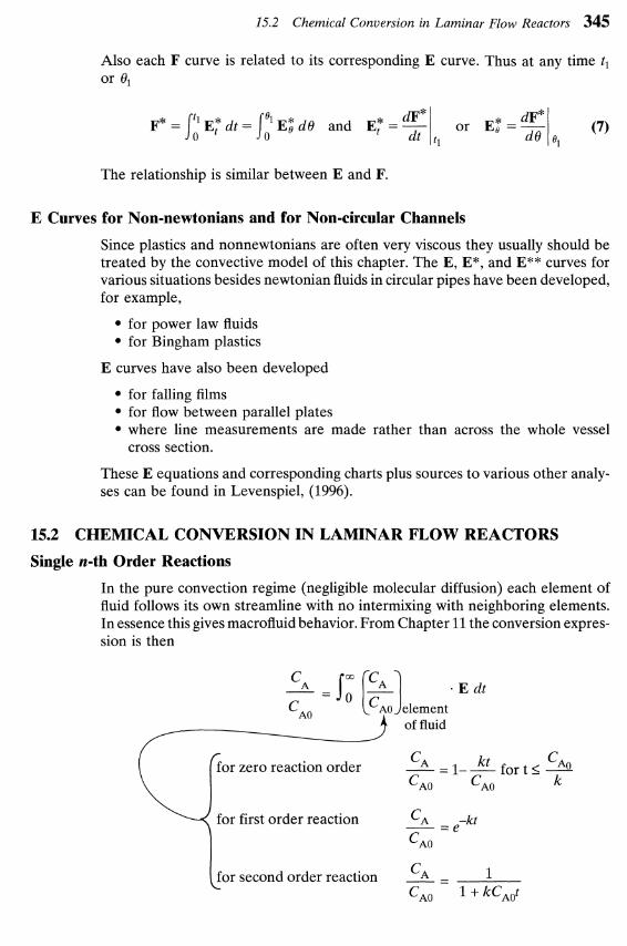
In the pure convection regime (negligible molecular diffusion) each element of fluid follows its own streamline with no intermixing with neighboring elements. In essence this gives macrofluid behavior. From Chapter 11 the conversion expression is then

for zero reaction order CA -- kt C ~ O -I-- f o r t s -- CAO CAO k

for first order reaction r CA C~~ = e -kt

c~ - for second order reaction - 1 - 1

CAO 1 + kCAOt


For zero-order reaction of a newtonian in laminar flow in a pipe, integration of Eq. 8 gives

For first-order reaction of a newtonian in laminar flow in a pipe,

where ei(y) is the exponential integral, see Chapter 16. For second-order reaction of a newtonian in laminar flow in a pipe:

These performance expressions were first developed by Bosworth (1948) for zero order, by Denbigh (1951) for second order, and by Cleland and Wilhelm (1956) for first order reactions. For other kinetics, channel shapes, or types of fluids insert the proper terms in the general performance expression and integrate.

Comments

(a) Test for the R T D curve. Proper RTD curves must satisfy the material balance checks (calculated zero and first moments should agree with measured values)

E . ~ B = 1 and 1' BE,dB = 1 0 0

(12)

The E curves of this chapter, for non-newtonians and all shapes of channels, all meet this requirement. All the E* and E** curves of this chapter do not; however, their transforms to E do.

(b) The variance and other R T D descriptors. The variance of all the E curves of this chapter is finite; but it is infinite for all the E* and E** curves. So be sure you know which curve you are dealing with.

In general the convection model E curve has a long tail. This makes the measurement of its variance unreliable. Thus cr2 is not a useful parameter for convection models and is not presented here.

The breakthrough time 8, is probably the most reliably measured and most useful descriptive parameter for convection models, so it is widely used.

(c) Comparison with plug flow for nth-order reaction is shown in Fig. 15.10.

This graph shows that even at high XA convective flow does not drastically lower reactor performance. This result differs from the dispersion and tanks-in-series models (see Chapters 13 and 14).

15.2 Chemical Conversion in Laminar Flow Reactors 347

Convection versus -

1 I / I I /

Figure 15.10 Convective flow lowers conversion compared to plug flow.

Multiple Reaction in Laminar Flow

Consider a two-step first-order irreversible reactions in series

Because laminar flow represents a deviation from plug flow, the amount of intermediate formed will be somewhat less than for plug flow. Let us examine this situation.

PFR

LFR

PFR

LFR

M FR

Figure 15.11 Typical product distribution curves for laminar flow compared with the curves for plug flow (Fig. 8.13) and mixed flow (Fig. 8.14).


The disappearance of A is given by the complicated Eq. 10, and the formation and disappearance of R is given by an even more complicated equation. Devel- oping the product distribution relationship, solving numerically, and comparing the results with those for plug flow and for mixed flow gives Fig. 15.11; see Johnson (1970) and Levien and Levenspiel (1998).

This graph shows that the LFR gives a little less intermediate than does the PFR, about 20% of the way from the PFR to the MFR.

We should be able to generalize these findings to other more complex reaction systems, such as for two component multistep reactions; to polymerizations; and to nowNewtonian power law fluids.

REFERENCES

Ananthakrishnan, V., Gill, W. N., and Barduhn, A. J., AIChE J., 11,1063 (1965). Bosworth, R. C. L., Phil. Mag., 39, 847 (1948). Cleland, F. A., and Wilhelm, R. H., AIChE J., 2, 489 (1956). Denbigh, K. G., J. Appl. Chem., 1,227 (1951). Johnson, M. M., Ind. Eng. Chem. Fundamentals, 9, 681 (1970). Levenspiel, O., Chemical Reactor Omnibook, Chap. 68, OSU Bookstores, Corvallis, OR

97339, 1996. Levien, K. L., and Levenspiel, O., Chem. Eng. Sci., 54, 2453 (1999).

PROBLEMS

A viscous liquid is to react while passing through a tubular reactor in which flow is expected to follow the convection model. What conversion can we expect in this reactor if plug flow in the reactor will give 80% conversion?

15.1. Reaction follows zero-order kinetics.

15.2. Reaction is second order.

15.3. Assuming plug flow we calculate that a tubular reactor 12 m long would give 96% conversion of A for the second-order reaction A --+ R. However, the fluid is very viscous, and flow will be strongly laminar, thus we expect the convection model, not the plug flow model, to closely represent the flow. How long should we make the reactor to insure 96% conversion of A?

15.4. Aqueous A (C,, = 1 mollliter) with physical properties close to water (p = 1000 kg/m3, CB = m2/s) reacts by a first-order homogeneous reaction (A -t R, k = 0.2 s-I) as it flows at 100 mm/s through a tubular reactor (d, = 50 mm, L = 5 m). Find the conversion of A in the fluid leaving this reactor.

Problems 349

15.5. Aqueous A (CAO = 50 mol/m3) with physical properties close to water ( p = 1000 kg/m3, !3 = m2/s) reacts by a second-order reaction (k =

m3/mol. s) as it flows at 10 mmls through a tubular reactor (d, = 10 mm, L = 20 m). Find the conversion of reactant A from this reactor.

15.6. We want to model the flow of fluid in a flow channel. For this we locate three measuring points A, B, and C, 100 m apart along the flow channel. We inject tracer upstream of point A, fluid flows past points A, B, and C with the following results:

At A the tracer width is 2 m At B the tracer width is 10 m At C the tracer width is 14 m

What type of flow model would you try to use to represent this flow: dispersion, convective, tanks-in-series, or none of these? Give a reason for your answer.

Chapter 1

Earliness of Mixing, Segregation, and RTD

The problem associated with the mixing of fluids during reaction is important for extremely fast reactions in homogeneous systems, as well as for all heterogeneous systems. This problem has two overlapping aspects: first, the degree o f segregation of the fluid, or whether mixing occurs on the microscopic level (mixing of individual molecules) or the macroscopic level (mixing of clumps, groups, or aggregates of molecules); and second, the earliness o f mixing, or whether fluid mixes early or late as it flows through the vessel.

These two concepts are intertwined with the concept of RTD, so it becomes rather difficult to understand their interaction. Please reread the first few pages of Chapter 11 where these concepts are introduced and discussed.

In this chapter we first treat systems in which a single fluid is reacting. Then we treat systems in which two fluids are contacted and reacted.

16.1 SELF-MIXING OF A SINGLE FLUID

Degree of Segregation

The normally accepted state of a liquid or gas is that of a microfluid, and all previous discussions on homogeneous reactions have been based on the assumption. Let us now consider a single reacting macrofluid being processed in turn in batch, plug flow, and mixed flow reactors, and let us see how this state of aggregation can result in behavior different from that of a microfluid.

Batch Reactor. Let the batch reactor be filled with a macrofluid containing reactant A. Since each aggregate or packet of macrofluid acts as its own little batch reactor, conversion is the same in all aggregates and is in fact identical to what would be obtained with a microfluid. Thus for batch operations the degree of segregation does not affect conversion or product distribution.

Plug Flow Reactor. Since plug flow can be visualized as a flow of small batch reactors passing in succession through the vessel, macro- and microfluids act

16.1 Self-Mixing of a Single Fluid 351

Individual molecules lose their identity, and reactant concentration in uniform throughout

Figure 16.1 Difference in behavior i

flow reactors.

Each aggregate retains its identity and acts as a batch reactor; reactant concentration varies from aggregate to aggregate

3f microfluids and macrofluids in mixed

alike. Consequently the degree of segregation does not influence conversion or product distribution.

Mixed Flow Reactor-Microfluid. When a microfluid containing reactant A is treated as in Fig. 16.1, the reactant concentration everywhere drops to the low value prevailing in the reactor. No clump of molecules retains its high initial concentration of A. We may characterize this by saying that each molecule loses its identity and has no determinable past history. In other words, by examining its neighbors we cannot tell whether a molecule is a newcomer or an old-timer in the reactor.

For this system the conversion of reactant is found by the usual methods for homogeneous reactions, or

or, with no density changes,

where 7 is the mean residence time of fluid in the reactor.

Mixed Flow Reactor-Macrofluid. When a macrofluid enters a mixed flow reactor, the reactant concentration in an aggregate does not drop immediately to a low value but decreases in the same way as it would in a batch reactor. Thus a molecule in a macrofluid does not lose its identity, its past history is not unknown, and its age can be estimated by examining its neighboring molecules.

The performance equation for a macrofluid in a mixed flow reactor is given by Eq. 11.13 as

- CA CA 1 - X A - --=I (-) Edt CAO 0 CAO batch

352 Chapter 16 Earliness of Mixing, Segregation, and RTD

where

V e-t/i E dt = - e-"/V dt = - dt v t

Replacing Eq. 3 in Eq. 2 gives

This is the general equation for determining conversion of macrofluids in mixed flow reactors, and it may be solved once the kinetics of the reaction is given. Consider various reaction orders.

For a zero-order reaction in a batch reactor, Chapter 3 gives

Inserting into Eq. 4 and integrating gives

For afirst-order reaction in a batch, reactor Chapter 3 gives

On replacing into Eq. 4 we obtain

which on integration gives the expression for conversion of a macrofluid in a mixed flow reactor

This equation is identical to that obtained for a microfluid; for example, see Eq. 5.14a. Thus we conclude that the degree of segregation has no effect on conversion for first-order reactions.


For a second-order reaction of a single reactant in a batch reactor Eq. 3.16 gives

On replacing into Eq. 4 we find

and by letting a = l /CAokt and converting into reduced time units 0 = tlt, this expression becomes

This is the conversion expression for second-order reaction of a macrofluid in a mixed flow reactor. The integral, represented by ei(a) is called an exponential integral. It is a function alone of a , and its value is tabulated in a number of tables of integrals. Table 16.1 presents a very abbreviated set of values for both ei(x) and Ei(x). We will refer to this table later in the book.

Table 16.1 Two of the Family of Exponential Integrals

x2 x3 ~ i ( x ) = eYdu=0 .57721+lnx+x+-+-+ . .

Here are two useful 2 - 2 ! 3 .3 exponential integrals x2 x3 -0.57721-lnx+x-- +-- . . .

2.2! 3.3!

x Ei(x) ei(x) x Ei (x)

0 -to + m 0.2 -0.8218 0.01 -4.0179 4.0379 0.3 -0.3027 0.02 -3.3147 3.3547 0.5 0.4542 0.05 -2.3679 2.4679 1.0 1.8951 0.1 -1.6228 1.8229 1.4 3.0072

Reference: "Tables of Sines, Cosines and Exponential Integrals," Vols. I and 11, by WPA, for NBS (1940).


Equation 8 may be compared with the corresponding expression for microfluids, Eq. 5.14

For an nth-order reaction the conversion in a batch reactor can be found by the methods of Chapter 3 to be

Insertion into Eq. 4 gives the conversion for an nth-order reaction of a macrofluid.

Difference in Performance: Early or Late Mixing, Macro- or Microfluids, PFR or MFR

Figure 16.2 illustrates the difference in performance of macrofluids and microfluids in mixed flow reactors, and they show clearly that a rise in segregation improves reactor performance for reaction orders greater than unity but lowers performance for reaction orders smaller than unity. Table 16.2 was used in preparing these charts.

Early and Late Mixing of Fluids

Each flow pattern of fluid through a vessel has associated with it a definite clearly defined residence time distribution (RTD), or exit age distribution function E. The converse is not true, however. Each RTD does not define a specific flow pattern; hence, a number of flow patterns-some with earlier mixing, others with later mixing of fluids-may be able to give the same RTD.

Idealized Pulse RTD. Reflection shows that the only pattern of flow consistent with this RTD is one with no intermixing of fluid of different ages, hence, that of plug flow. Consequently it is immaterial whether we have a micro- or macrofluid. In addition the question of early or late mixing of fluid is of no concern since there is no mixing of fluid of different ages.

Exponential Decay RTD. The mixed flow reactor can give this RTD. However, other flow patterns can also give this RTD, for example, a set of parallel plug flow reactors of proper length, a plug flow reactor with sidestreams, or a combina- tion of these. Figure 16.3 shows a number of these patterns. Note that in patterns a and b entering fluid elements mix immediately with material of different ages, while in patterns c and d no such mixing occurs. Thus patterns a and b represent the microfluid, while patterns c and d represent the macrofluid.


Figure 16.2 Comparison of performance of mixed flow reactors treating micro- and macrofluids; for zero- and second-order reactions with = 0.

Arbitrary RTD. In extending this argument we see that when the RTD is close to that of plug flow, then the state of segregation of fluid as well as early or late mixing of fluid has little effect on conversion. However, when the RTD approaches the exponential decay of mixed flow, then the state of segregation and earliness of mixing become increasingly important.

For any RTD one extreme in behavior is represented by the macrofluid and the latest mixing microfluid, and Eq. 2 gives the performance expression for this case. The other extreme is represented by the earliest mixing microfluid. The performance expression for this case has been developed by Zwietering (1959) but is difficult to use. Although these extremes give the upper and lower bound to the expected conversion for real vessels, it is usually simpler and preferable to develop a model to reasonably approximate the real vessel and then calculate conversions from this model. This is what actually was done in developing Fig. 13.20 for second-order reaction with axial dispersion. There we assumed that the same extent of mixing occurs along the whole vessel.

% Ch

Table 16.2 Conversion Equations for Macrofluids and Microfluids with E = 0 in Ideal Reactors

Plug Flow Mixed Flow

Microfluid or Macrofluid Microfluid Macrofluid

General kinetics - c = ' Jm (") e - l l ~ dt CO 7 0 CO batch

nth-order reaction

( R = Ci;-'k~)

First-order reaction

( R = k7)

Second-order reaction c - 1 -- c - - 1 + m C, l + R co 2R -

C - ellR - - -ei (k)

( R = Cok7) co R = - - 1 co R C

- -

R = C i - ' k ~ , reaction rate group for nth-order reaction, a time or capacity factor. T = i since E = 0 throughout.


/ , v ! ! l - * \ Mixedflow - :---+

- F d ;<C---;T \\ 1

Set of parallel plug flow

(c)

Side leaving ,- plug flow

L S i d e feeding plug flow

(6) (d )

Figure 16.3 Four contacting patterns which can all give the same exponential decay RTD. Cases a and b represent the earliest possible mixing while cases c and d represent the latest possible mixing of fluid elements of different ages.

Summary of Findings for a Single Fluid

1. Factors affecting the performance of a reactor. In general we may write

kinetics, RTD, degree of segregation, Performance: XA or cp ( g ) = ( earliness of mixing

2. Effect of kinetics, or reaction order. Segregation and earliness of mixing affect the conversion of reactant as follows

For n > 1 - . . Xmacro and Xmicro, late > Xmicro, early

For n < 1 the inequality is reversed, and for n = 1 conversion is unaffected by these factors. This result shows that segregation and late mixing improves conversion for n > 1, and decreases conversion for n < 1.

3. Effect of mixing factors for nonfirst-order reactions. Segregation plays no role in plug flow; however, it increasingly affects the reactor performance as the RTD shifts from plug to mixed flow.

4. Effect of conversion level. At low conversion levels X, is insensitive to RTD, earliness of mixing, and segregation. At intermediate conversion levels, the RTD begins to influence XA; however, earliness and segregation still have little effect. This is the case of Example 16.1. Finally, at high conversion levels all these factors may play important roles.

5. Effect on product distribution. Although segregation and earliness of mixing can usually be ignored when treating single reactions, this often is not so with multiple reactions where the effect of these factors on product distribution can be of dominating importance, even at low conversion levels.


As an example consider free-radical polymerization. When an occasional free radical is formed here and there in the reactor it triggers an extremely rapid chain of reactions, often thousands of steps in a fraction of a second. The local reaction rate and conversion can thus be very high. In this situation the immediate surroundings of the reacting and growing molecules-and hence the state of segregation of the fluid-can greatly affect the type of polymer formed.

EFFECT OF SEGREGATION AND EARLINESS OF MIXING ON CONVERSION

A second-order reaction occurs in a reactor whose RTD is given in Fig. E16.1. Calculate the conversion for the flow schemes shown in this figure. For simplicity take C, = 1, k = 1, and r = 1 for each unit.

Microfluid co =-, I

Macrofluid

3 I :,

To approx~mate the

(c)

Figure E16.1 ( a ) Microfluid, early mixing at molecular level; (b) Mi- crofluid, fairly late mixing at molecular level; (c) Microfluid, late mixing at molecular level; ( d ) Mac~ofluid, early mixing of elements; ( e ) Mac- rofluid, late mixing of elements.


I SOLUTION

Scheme A. Referring to Fig. E16.1~ we have for the mixed flow reactor

For the plug flow reactor

Scheme B. Referring to Fig. E16.lb, we have for the plug flow reactor

For the mixed reactor

Micro-fairly late: C; = 0.366

Scheme C, D, and E. From Fig. 12.1 the exit age distribution function for the two equal-size plug-mixed flow reactor system is

2 - E = = el-2t1t t 1 , when T > - t t 2

t 1 = 0, when Y < -

t 2


I Thus Eq. 3 becomes

With the mean residence time in the two-vessel system f = 2 min, this becomes

l and replacing 1 + t by x we obtain the exponential integral

I From the table of integrals in Table 16.1 we find ei(2) = 0.048 90 from which

Micro-late, and macro-late or early: C" = 0.362

The results of this example confirm the statements made above: that macrofluids and late mixing microfluids give higher conversions than early mixing microfluids for reaction orders greater than unity. The difference is small here because the conversion levels are low; however, this difference becomes more important as conversion approaches unity.

Extensions for a Single Fluid

Partial Segregation. There are various ways of treating intermediate extents of segregation, for example,

Intensity of segregation model-Danckwerts (1958) Coalescence model-Curl (1963), Spielman and Levenspiel (1965) Two environment and melting ice cube models-Ng and Rippin (1965) and

Suzuki (1970)

These approaches are discussed in Levenspiel (1972).

The Life of an Element of Fluid. Let us estimate how long a fluid element retains its identity. First, all large elements are broken into smaller elements by stretching or folding (laminar behavior) or by turbulence generated by baffles, stirrers, etc., and mixing theory estimates the time needed for this breakup.

Small elements lose their identity by the action of molecular diffusion, and the Einstein random walk analysis estimates this time as

(size of element)' - d2lement t = --

( diffusion \ !ZJ {coefficient)

16.2 Mixing of Two Miscible Fluids 361

Thus an element of water 1 micron in size would lose its identity in a very short time, approximately

t = ~ m ) ~

= sec cm2/sec

while an element of viscous polymer 1.0 mm in size and 100 times as viscous as water (10-30 W motor oil at room temperature) would retain its identity for a long time, roughly

t = (10-I ~ m ) ~

= lo5 sec .=; 30 hr cm2/sec

In general, then, ordinary fluids behave as microfluids except for very viscous materials and for systems in which very fast reactions are taking place.

The concept of micro- and macrofluids is of particular importance in heterogeneous systems because one of the two phases of such systems usually approxi- mates a macrofluid. For example, the solid phase of fluid-solid systems can be treated exactly as a macrofluid because each particle of solid is a distinct aggregate of molecules. For such systems, then, Eq. 2 with the appropriate kinetic expression is the starting point for design.

In the chapters to follow we apply these concepts of micro- and macrofluids to heterogeneous systems of various kinds.

16.2 MIXING OF TWO MISCIBLE FLUIDS

Here we consider one topic, the role of the mixing process when two completely miscible reactant fluids A and B are brought together. When two miscible fluids A and B are mixed, we normally assume that they first form a homogeneous mixture which then reacts. However, when the time required for A and B to become homogeneous is not short with respect to the time for reaction to take place, reaction occurs during the mixing process, and the problem of mixing becomes important. Such is the case for very fast reactions or with very viscous reacting fluids.

To help understand what occurs, imagine that we have A and B available, each first as a microfluid, and then as a macrofluid. In one beaker mix micro A with micro B, and in another beaker mix macro A with macro B and let them react. What do we find? Micro A and B behave in the expected manner, and reaction occurs. However, on mixing the macrofluids no reaction takes place because molecules of A cannot contact molecules of B. These two situations are illustrated in Fig. 16.4. So much for the treatment of the two extremes in behavior.

Now a real system acts as shown in Fig. 16.5 with regions of A-rich fluid and regions of B-rich fluid.

Though partial segregation requires an increase in reactor size, this is not the only consequence. For example, when reactants are viscous fluids, their mixing in a stirred tank or batch reactor often places layers or "streaks" of one fluid next to the other. As a result reaction occurs at different rates from point to


A B A B C-

reaction occurs no reaction occurs

Figure 16.4 Difference in behavior of microfluids and macrofluids in the reaction of A and B.

point in the reactor, giving a nonuniform product which may be commercially unacceptable. Such is the case in polymerization reactions in which monomer must be intimately mixed with a catalyst. For reactions such as this, proper mixing is of primary importance and often the rate of reaction and product uniformity correlate well with the mixing energy input to the fluid.

For fast reactions the increase in reactor size needed because of segregation is of secondary importance while other effects become important. For example, if the product of reaction is a solid precipitate, the size of the precipitate particles may be influenced by the rate of intermixing of reactants, a fact that is well known from the analytical laboratory. As another example, hot gaseous reaction mixtures may contain appreciable quantities of a desirable compound because of favorable thermodynamic equilibrium at such temperatures. To reclaim this component the gas may have to be cooled. But, as is often the case, a drop in temperature causes an unfavorable shift in equilibrium with essentially complete disappearance of desired material. To avoid this and to "freeze" the composition of hot gases, cooling must be very rapid. When the method of quenching used involves mixing the hot gases with an inert cold gas, the success of such a procedure is primarily dependent on the rate at which segregation can be de- stroyed. Finally the length, type, and temperature of a burning flame, the combus- tion products obtained, the noise levels of jet engines, and the physical properties of polymers as they are affected by the molecular weight distribution of the

A r A-rich region

L ~ - r i c h region B / B-rich region

Figure 16.5 Partial segregation in the mixing of two miscible fluids in a reactor.

16.2 Mixing of Two Miscible Fluids 363

material are some of the many phenomena that are closely influenced by the rate and intimacy of fluid mixing.

Product Distribution in Multiple Reactions

When multiple reactions take place on mixing two reactant fluids and when these reactions proceed to an appreciable extent before homogeneity is attained, segregation is important and can affect product distribution.

Consider the homogeneous-phase competitive consecutive reactions

occurring when A and B are poured into a batch reactor. If the reactions are slow enough so that the contents of the vessel are uniform before reaction takes place, the maximum amount of R formed is governed by the k,lk, ratio. This situation, treated in Chapter 8, is one in which we may assume microfluid behavior. If, however, the fluids are very viscous or if the reactions are fast enough, they will occur in the narrow zones between regions of high A concentration and high B concentration. This is shown in Fig. 16.6. The zone of high reaction rate will contain a higher concentration of R than the surrounding fluid. But from the qualitative treatment of this reaction in Chapter 8 we know that any nonhonrogeneity in A and R will depress formation of R. Thus partial segregation of reaotants will depress the formation of intermediate.

For increased reaction rate, the zone of reaction narrows, and in the limit, for an infinitely fast reaction, becomes a boundary surface between the A-rich and

L- High-reaction-rate zone containing a high concentration of R

Figure 16.6 When reaction rate is very high, zones of nonhomogeneity exist in a reactor. This condition is detrimental to obtaining high yields of intermediate R from the reactions


Fast reaction (some R formed)

Infinitely fast reaction (no R formed)

A-r1ch 'a region reglon A-rich \ regi0n region

Reaction zone

J Reaction zone

I is a plane

A-rich B-rich region I

I region

!

Distance Distance

Figure 16.7 Concentration profiles of the components of the reactions

at a representative spot in the reactor between A-rich and B-rich fluid for a very fast and for an infinitely fast reaction.

B-rich regions. Now R will only be formed at this plane. What will happen to it? Consider a single molecule of R formed at the reaction plane. If it starts its random wanderings (diffusion) into the A zone and never moves back into the B zone, it will not react further and will be saved. However, if it starts off into the B zone or if at any time during its wanderings it moves through the reaction plane into the B zone, it will be attacked by B to form S. Interestingly enough, from probabilities associated with a betting game treated by Feller (1957), we can show that the odds in favor of a molecule of R never entering the B zone become smaller and smaller as the number of diffusion steps taken by a molecule gets larger and larger. This finding holds, no matter what pattern of wanderings is chosen for the molecules of R. Thus we conclude that no R is formed. Looked at from the point of view of Chapter 8, an infinitely fast reaction gives a maximum nonhomogeneity of A and R in the mixture, resulting in no R being formed. Figure 16. 7 shows the concentration of materials at a typical reaction interface and illustrates these points.

References 365

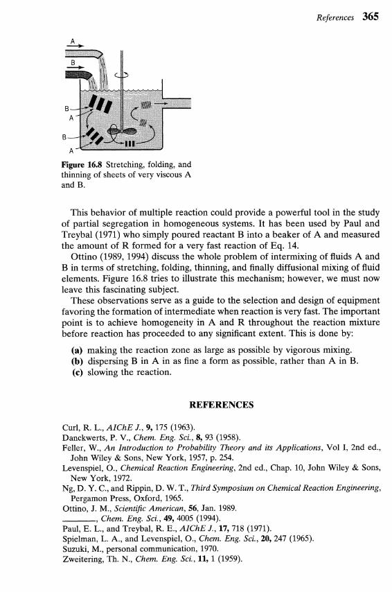
Figure 16.8 Stretching, folding, and thinning of sheets of very viscous A and B.

This behavior of multiple reaction could provide a powerful tool in the study of partial segregation in homogeneous systems. It has been used by Paul and Treybal(1971) who simply poured reactant B into a beaker of A and measured the amount of R formed for a very fast reaction of Eq. 14.

Ottino (1989, 1994) discuss the whole problem of intermixing of fluids A and B in terms of stretching, folding, thinning, and finally diffusional mixing of fluid elements. Figure 16.8 tries to illustrate this mechanism; however, we must now leave this fascinating subject.

These observations serve as a guide to the selection and design of equipment favoring the formation of intermediate when reaction is very fast. The important point is to achieve homogeneity in A and R throughout the reaction mixture before reaction has proceeded to any significant extent. This is done by:

(a) making the reaction zone as large as possible by vigorous mixing. (b) dispersing B in A in as fine a form as possible, rather than A in B. (c) slowing the reaction.

REFERENCES

Curl, R. L., AZChE J . , 9, 175 (1963). Danckwerts, P. V., Chem. Eng. Sci., 8, 93 (1958). Feller, W., An Introduction to Probability Theory and its Applications, Vol I , 2nd ed.,

John Wiley & Sons, New York, 1957, p. 254. Levenspiel, O., Chemical Reaction Engineering, 2nd ed., Chap. 10, John Wiley & Sons,

New York, 1972. Ng, D. Y. C., and Rippin, D. W. T., Third Symposium on Chemical Reaction Engineering,

Pergamon Press, Oxford, 1965. Ottino, J. M., Scientific American, 56, Jan. 1989. -, Chem. Eng. Sci., 49, 4005 (1994). Paul, E. L., and Treybal, R. E., AZChE J., 17,718 (1971). Spielman, L. A., and Levenspiel, O., Chem. Eng. Sci., 20,247 (1965). Suzuki, M., personal communication, 1970. Zweitering, Th. N., Chem. Eng. Sci., 11, 1 (1959).

Chapter 15 The Convection Model for Laminar Flo Chemical reaction engineering...340 Chapter 15 The...

Documents

Transcript of Chapter 15 The Convection Model for Laminar Flo Chemical reaction engineering...340 Chapter 15 The...